A Designed Thresholding Operator for Low-Rank Matrix Completion

Abstract

In this paper, a new thresholding operator, namely, designed thresholding operator, is designed to recover the low-rank matrices. With the change of parameter in designed thresholding operator, the designed thresholding operator can apply less bias to the larger singular values of a matrix compared with the classical soft thresholding operator. Based on the designed thresholding operator, an iterative thresholding algorithm for recovering the low-rank matrices is proposed. Numerical experiments on some image inpainting problems show that the proposed thresholding algorithm performs effectively in recovering the low-rank matrices.

1. Introduction

In recent years, the problem of recovering an unknown low-rank matrix from its limited number of observed entries has been actively studied in many scientific applications such as Netflix problem [1], image processing [2], system identification [3], video denoising [4], signal processing [5], subspace learning [6], and so on. In mathematics, this problem can be modeled by the following low-rank matrix completion problem:

$$\underset{\mathbf{X}\in {\mathbb{R}}^{m\times n}}{min}\mathrm{rank}\left(\mathbf{X}\right)\mathrm{s}.\mathrm{t}.{\mathbf{X}}_{i,j}={\mathbf{M}}_{i,j},\forall (i,j)\in \Omega ,$$

(1)

where $\Omega \subset \{1,2,\cdots ,m\}\times \{1,2,\cdots ,n\}$ is the set of indices of observed entries. Without loss of generality, throughout this paper, we assume that $m\le n$. If we summarize the observed entries via ${\mathcal{P}}_{\Omega }\left(\mathbf{M}\right)$, where the projection ${\mathcal{P}}_{\Omega }:{\mathbb{R}}^{m\times n}\to {\mathbb{R}}^{m\times n}$ is defined by

$${\left[{\mathcal{P}}_{\Omega }\left(\mathbf{X}\right)\right]}_{i,j}=\left\{\begin{array}{cc}{\mathbf{X}}_{i,j},\hfill & (i,j)\in \Omega ;\hfill \\ 0,\hfill & \mathrm{otherwise},\hfill \end{array}\right.$$

the low-rank matrix completion problem (1) can be rewritten as

$$\underset{\mathbf{X}\in {\mathbb{R}}^{m\times n}}{min}\mathrm{rank}\left(\mathbf{X}\right)\mathrm{s}.\mathrm{t}.{\mathcal{P}}_{\Omega }\left(\mathbf{X}\right)={\mathcal{P}}_{\Omega }\left(\mathbf{M}\right).$$

(2)

Unfortunately, the problem (2) is NP-hard and all known algorithms for exactly solving it are time doubly exponential in both theory and practice [1,7]. To overcome such a difficulty, many researchers (e.g., [1,3,5,8,9,10]) have suggested to relax the rank function $\mathrm{rank}\left(\mathbf{X}\right)$ by the nuclear norm ${\parallel \mathbf{X}\parallel }_{*}$, which leads to the following nuclear norm minimization problem:

$$\underset{\mathbf{X}\in {\mathbb{R}}^{m\times n}}{min}{\parallel \mathbf{X}\parallel }_{*}\mathrm{s}.\mathrm{t}.{\mathcal{P}}_{\Omega }\left(\mathbf{X}\right)={\mathcal{P}}_{\Omega }\left(\mathbf{M}\right),$$

(3)

where ${\parallel \mathbf{X}\parallel }_{*}={\sum }_{i=1}^m{\sigma }_i\left(\mathbf{X}\right)$ denotes the nuclear norm of matrix $\mathbf{X}\in {\mathbb{R}}^{m\times n}$, and ${\sigma }_i\left(\mathbf{X}\right)$, $i=1,\cdots ,m$, are the singular values of $\mathbf{X}\in {\mathbb{R}}^{m\times n}$.

The nuclear norm ${\parallel \mathbf{X}\parallel }_{*}$, as a convex relaxation of the rank function $\mathrm{rank}\left(\mathbf{X}\right)$, can be considered as the best convex approximation of the rank function $\mathrm{rank}\left(\mathbf{X}\right)$. In theory, Candès et al. [1,11] have proved that, if the observed entries are selected uniformly at random, the unknown low-rank matrix can be exactly recovered with high probability by solving the problem (2). As a convex optimization problem, the problem (2) can be solved by using the semidefinite programming solvers such as SeDuMi [12] and SDPT3 [13]. However, these algorithms are unsuitable to handle the large size problems due to the high computational cost and the memory requirements. Different from the semidefinite programming solvers, the regularized version of the problem (2), i.e.,

$$\underset{\mathbf{X}\in {\mathbb{R}}^{m\times n}}{min}\left\{\frac{1}{2}\parallel {\mathcal{P}}_{\Omega }\left(\mathbf{X}\right)-{\mathcal{P}}_{\Omega }{\left(\mathbf{M}\right)\parallel }_F^2+\lambda {\parallel \mathbf{X}\parallel }_{*}\right\}$$

(4)

has been frequently studied in the literature to solve the large-scale matrix completion, where $\lambda >0$ is a regularization parameter representing the tradeoff between error and nuclear norm. There are many algorithms proposed to solve the problem (3). The most popular algorithms include the singular value thresholding (SVT) algorithm [8], accelerated proximal gradient (APG) algorithm [14], linearized augmented lagrangian and alternating direction methods [15], and so on. These algorithms are all based on the soft thresholding operator [16] to recover the unknown low-rank matrices. Although the problem (4) possesses many algorithmic advantages, these iterative soft thresholding version algorithms tend to have the bias on shrinking all the singular values of matrices, and sometimes result in over-penalization as the $l_1$-norm in compressed sensing.

To reduce the bias, in this paper we design a new thresholding operator, namely, designed thresholding operator, to recover the low-rank matrices, which has less bias than the soft thresholding operator. The numerical experiments on some low-rank matrix completion problems show that the proposed thresholding operator performs efficiently in recovering the low-rank matrices.

This paper is organized as follows. In Section 2, we give the definition of the designed thresholding operator, and study some properties for the designed thresholding operator. In Section 3, an iterative thresholding algorithm based on the designed thresholding operator is generated to recover the low-rank matrices. In Section 4, some numerical experiments are presented to verify the effectiveness of the proposed algorithm. Finally, we draw some conclusions in Section 5.

2. Designed Thresholding Operator

In this section, we first review the classical soft thresholding operator [16], and then design a new thresholding operator, namely, designed thresholding operator, to recover the low-rank matrices.

2.1. Soft Thresholding Operator

For any fixed $\lambda >0$ and $t\in \mathbb{R}$, the soft thresholding operator [16] is defined as

$$s_{\lambda }\left(t\right)=max\left\{\left|t\right|-\lambda ,0\right\}\mathrm{sign}\left(t\right),$$

(5)

which can be explained by the fact that it is the proximity operator of $\left|x\right|$, i.e.,

$$s_{\lambda }\left(t\right):=arg\underset{x\in \mathbb{R}}{min}\left\{\frac{1}{2}{(x-t)}^2+\lambda \left|x\right|\right\}.$$

(6)

The soft thresholding operator plays a significant role in solving problem (4). However, it has the biased estimation and sometimes results in over-penalization. The behavior of the soft thresholding operator is plotted in Figure 1, and we can see that the bias between t and soft thresholding operator $s_{\lambda }\left(t\right)$ equals to $\lambda$.

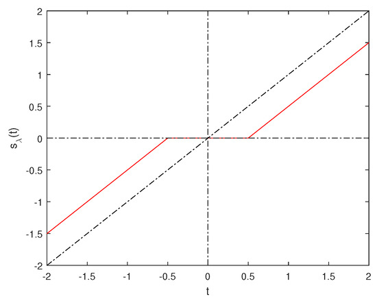
Figure 1. Plot of the soft thresholding operator $s_{\lambda }\left(t\right)$ with $\lambda =0.5$.

2.2. Designed Thresholding Operator

To reduce the bias, in this subsection we design a new thresholding operator, namely, designed thresholding operator, to recover the low-rank matrices.

Definition 1. 

(Designed thresholding operator) For any fixed $\lambda >0$, $c\ge 0$ and $t\in \mathbb{R}$, the designed thresholding operator is defined as

$$r_{c,\lambda }\left(t\right)=max\left\{\left|t\right|-\frac{\lambda (c+\lambda )}{c+\left|t\right|},0\right\}\mathrm{sign}\left(t\right).$$

(7)

According to Definition 1, we immediately obtain the following Property 1, which shows that the designed thresholding operator has less bias to the larger coefficients than the soft thresholding operator.

Property 1. 

For any $c\in [0,+\infty )$, the bias $t-r_{c,\lambda }\left(t\right)$ approaches zero as the magnitude of t increases.

Proof. 

Without loss of generality, we assume $t\ge 0$. Then, we have $t-r_{c,\lambda }\left(t\right)\le \lambda$ for any $t\ge 0$, and $t-r_{c,\lambda }\left(t\right)=\frac{\lambda (c+\lambda )}{c+t}$ for any $t\ge \lambda$. It is easy to verify that $t-r_{c,\lambda }\left(t\right)=\frac{\lambda (c+\lambda )}{c+t}\to 0$ if $t\to +\infty$. The proof is thus complete.    □

In addition, we can also observe that the designed thresholding operator approximates soft thresholding operator when $c\to +\infty$, i.e.,

$$\underset{c\to +\infty }{lim}{r}_{c,\lambda }=max\left\{\left|t\right|-\lambda ,0\right\}\mathrm{sign}\left(t\right).$$

The behaviors of the designed thresholding operator for some $c\ge 0$ with $\lambda =0.5$ are plotted in Figure 2. With the change of parameter $c>0$, the designed thresholding operator can apply less bias to the larger coefficients.

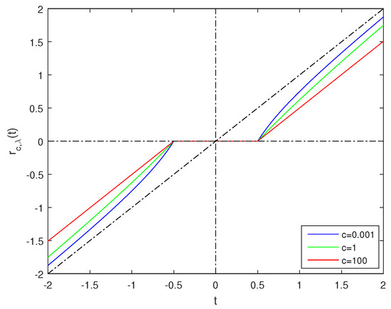
Figure 2. Plot of the designed thresholding operator $r_{c,\lambda }\left(t\right)$ for some c with $\lambda =0.5$.

According to ([17], Theorem 1), we immediately obtain the following Lemma 1, which shows that the designed thresholding operator is in fact the proximal mapping of a non-convex penalty function.

Lemma 1. 

The designed threshold operator $r_{c,\lambda }\left(t\right)$ is the proximal mapping of a penalty function $g\left(t\right)$, i.e.,

$$r_{c,\lambda }\left(t\right)=arg\underset{x\in \mathbb{R}}{min}\left\{\frac{1}{2}{(x-t)}^2+\lambda g\left(x\right)\right\},$$

(8)

where g is even, nondecreasing and continuous on $[0,+\infty )$, differentiable on $(0,+\infty )$, and nondifferentiable at $0$ with $\mathsf{\partial }g\left(0\right)=[-1,1]$. Moreover, g is concave on $[0,+\infty )$ and satisfies the triangle inequality.

Definition 2. 

(Matrix designed thresholding operator) Given a matrix $\mathbf{X}\in {\mathbb{R}}^{m\times n}$, let $\mathbf{X}=\mathbf{U}[\mathrm{Diag}\left({\left\{{\sigma }_i\left(\mathbf{X}\right)\right\}}_{1\le i\le m}\right),{\mathbf{0}}_{m\times (n-m)}]{\mathbf{V}}^{\top }$ be the singular value decomposition (SVD) of matrix $\mathbf{X}$, where $\mathbf{U}$ is a $m\times m$ unitary matrix, $\mathbf{V}$ is a $n\times n$ unitary matrix, ${\sigma }_i\left(\mathbf{X}\right)$ is the i-th largest singular value of $\mathbf{X}$, $\mathrm{Diag}\left({\left\{{\sigma }_i\left(\mathbf{X}\right)\right\}}_{1\le i\le m}\right)\in {\mathbb{R}}^{m\times m}$ is the diagonal matrix of the singular values of matrix $\mathbf{X}$ arranged in descending order ${\sigma }_1\left(\mathbf{X}\right)\ge {\sigma }_2\left(\mathbf{X}\right)\ge \cdots \ge {\sigma }_m\left(\mathbf{X}\right)\ge 0$, and ${\mathbf{0}}_{m\times (n-m)}$ is a $m\times (n-m)$ zero matrix. For any fixed $\lambda >0$ and $c\ge 0$, the matrix designed thresholding operator ${\mathcal{R}}_{c,\lambda }\left(\mathbf{X}\right)$ is defined as

$${\mathcal{R}}_{c,\lambda }\left(\mathbf{X}\right)=\mathbf{U}[\mathrm{Diag}\left({\left\{r_{c,\lambda }\left({\sigma }_i\left(\mathbf{X}\right)\right)\right\}}_{1\le i\le m}\right),{\mathbf{0}}_{m\times (n-m)}]{\mathbf{V}}^{\top },$$

(9)

where $r_{c,\lambda }(·)$ is defined in Definition 1.

For any matrix $\mathbf{X}\in {\mathbb{R}}^{m\times n}$, define the function $G:{\mathbb{R}}^{m\times n}\to {\mathbb{R}}_{+}$ as

$$G\left(\mathbf{X}\right)=\sum _{i=1}^{m}g\left({\sigma }_i\left(\mathbf{X}\right)\right),$$

(10)

where ${\mathbb{R}}_{+}:=[0,+\infty )$, we can get the following result.

Theorem 1. 

For any fixed $\lambda >0$ and $\mathbf{Y}\in {\mathbb{R}}^{m\times n}$, suppose that $\widehat{\mathbf{X}}\in {\mathbb{R}}^{m\times n}$ is the optimal solution of the problem

$$\underset{\mathbf{X}\in {\mathbb{R}}^{m\times n}}{min}\left\{\frac{1}{2}{\parallel \mathbf{X}-\mathbf{Y}\parallel }_F^2+\lambda G\left(\mathbf{X}\right)\right\}.$$

(11)

Then $\widehat{\mathbf{X}}$ can be expressed as

$$\widehat{\mathbf{X}}={\mathcal{R}}_{c,\lambda }\left(\mathbf{Y}\right).$$

(12)

Before we give the proof of Theorem 1, we need prepare the following Lemma 2 which plays the key rule for proving Theorem 1.

Lemma 2. 

(von Neumann’s trace inequality) For any matrices $\mathbf{X},\mathbf{Y}\in {\mathbb{R}}^{m\times n}$,

$$\mathrm{Tr}\left({\mathbf{X}}^T\mathbf{Y}\right)\le \sum _{i=1}^m{\sigma }_i\left(\mathbf{X}\right){\sigma }_i\left(\mathbf{Y}\right),$$

where ${\sigma }_1\left(\mathbf{X}\right)\ge {\sigma }_2\left(\mathbf{X}\right)\ge \cdots \ge {\sigma }_m\left(\mathbf{X}\right)$ and ${\sigma }_1\left(\mathbf{Y}\right)\ge {\sigma }_2\left(\mathbf{Y}\right)\ge \cdots \ge {\sigma }_m\left(\mathbf{Y}\right)$ are the singular values of $\mathbf{X}$ and $\mathbf{Y}$, respectively. The equality holds if and only if there exists unitary matrices $\mathbf{U}$ and $\mathbf{V}$ such that

$$\mathbf{X}=\mathbf{U}[\mathrm{Diag}\left({\left\{{\sigma }_i\left(\mathbf{X}\right)\right\}}_{1\le i\le m}\right),{\mathbf{0}}_{m\times (n-m)}]{\mathbf{V}}^T$$

and

$$\mathbf{Y}=\mathbf{U}[\mathrm{Diag}\left({\left\{{\sigma }_i\left(\mathbf{Y}\right)\right\}}_{1\le i\le m}\right),{\mathbf{0}}_{m\times (n-m)}]{\mathbf{V}}^T$$

are the SVDs of $\mathbf{X}$ and $\mathbf{Y}$, simultaneously.

Now, we give the proof of Theorem 1.

Proof. 

(of Theorem 1) By Lemma 2, we have

$$\begin{array}{cc}\hfill {\parallel \mathbf{X}-\mathbf{Y}\parallel }_F^2& =\mathrm{Tr}\left({\mathbf{X}}^T\mathbf{X}\right)-2\mathrm{Tr}\left({\mathbf{X}}^T\mathbf{Y}\right)+\mathrm{Tr}\left({\mathbf{Y}}^T\mathbf{Y}\right)\hfill \\ \hfill & =\sum _{i=1}^m{\sigma }_i^2\left(\mathbf{X}\right)-2\mathrm{Tr}\left({\mathbf{X}}^T\mathbf{Y}\right)+\sum _{i=1}^m{\sigma }_i^2\left(\mathbf{Y}\right)\hfill \\ \hfill & \ge \sum _{i=1}^m{\sigma }_i^2\left(\mathbf{X}\right)-2\sum _{i=1}^m{\sigma }_i\left(\mathbf{X}\right){\sigma }_i\left(Y\right)+\sum _{i=1}^m{\sigma }_i^2\left(\mathbf{Y}\right)\hfill \\ \hfill & =\sum _{i=1}^m{({\sigma }_i\left(\mathbf{X}\right)-{\sigma }_i\left(\mathbf{Y}\right))}^2.\hfill \end{array}$$

Notice that the equality holds if and only if $\mathbf{X}$ and $\mathbf{Y}$ share the same left and right unitary matrices, we assume that

$$\mathbf{X}=\mathbf{U}[\mathrm{Diag}\left({\left\{{\sigma }_i\left(\mathbf{X}\right)\right\}}_{1\le i\le m}\right),{\mathbf{0}}_{m\times (n-m)}]{\mathbf{V}}^T$$

and

$$\mathbf{Y}=\mathbf{U}[\mathrm{Diag}\left({\left\{{\sigma }_i\left(\mathbf{Y}\right)\right\}}_{1\le i\le m}\right),{\mathbf{0}}_{m\times (n-m)}]{\mathbf{V}}^T$$

are the SVDs of $\mathbf{X}$ and $\mathbf{Y}$, simultaneously. Therefore, it holds that

$${\parallel \mathbf{X}-\mathbf{Y}\parallel }_F^2=\sum _{i=1}^m{({\sigma }_i\left(\mathbf{X}\right)-{\sigma }_i\left(\mathbf{Y}\right))}^2,$$

and the problem (11) reduces to

$$\underset{{\sigma }_1\left(\mathbf{X}\right)\ge {\sigma }_2\left(\mathbf{X}\right)\ge \cdots \ge {\sigma }_m\left(\mathbf{X}\right)\ge 0}{min}\sum _{i=1}^m\left\{\frac{1}{2}{({\sigma }_i\left(\mathbf{X}\right)-{\sigma }_i\left(\mathbf{Y}\right))}^2+\lambda g\left({\sigma }_i\left(\mathbf{X}\right)\right)\right\}.$$

(13)

The objective function in (13) is separable, hence, solving the problem (13) is equivalent to solving the following n problems, for each $i=1,2,\cdots ,n$,

$$\underset{{\sigma }_i\left(\mathbf{X}\right)\ge 0}{min}\left\{\frac{1}{2}{({\sigma }_i\left(\mathbf{X}\right)-{\sigma }_i\left(\mathbf{Y}\right))}^2+\lambda g\left({\sigma }_i\left(\mathbf{X}\right)\right)\right\}.$$

(14)

Let ${\widehat{\sigma }}_i\left(\mathbf{X}\right)$ be the optimal solution of the problem (14), by Lemma 1, ${\widehat{\sigma }}_i\left(\mathbf{X}\right)$ can be expressed as

$${\widehat{\sigma }}_i\left(\mathbf{X}\right)=r_{c,\lambda }\left({\sigma }_i\left(\mathbf{Y}\right)\right).$$

(15)

Therefore, we can get the optimal solution $\widehat{\mathbf{X}}$ of the problem (11) as follows

$$\widehat{\mathbf{X}}=\mathbf{U}[\mathrm{Diag}\left({\left\{r_{c,\lambda }\left({\sigma }_i\left(\mathbf{Y}\right)\right)\right\}}_{1\le i\le m}\right),{\mathbf{0}}_{m\times (n-m)}]{\mathbf{V}}^{\top },$$

(16)

namely,

$$\widehat{\mathbf{X}}={\mathcal{R}}_{c,\lambda }\left(\mathbf{Y}\right).$$

This completes the proof.    □

3. Iterative Matrix Designed Thresholding Algorithm

In this section, we present an iterative thresholding algorithm to recover the low-rank matrices using the proposed designed thresholding operator.

Consider the following minimization problem:

$$\underset{\mathbf{X}\in {\mathbb{R}}^{m\times n}}{min}\left\{\frac{1}{2}{\parallel {\mathcal{P}}_{\Omega }\left(\mathbf{X}\right)-{\mathcal{P}}_{\Omega }\left(\mathbf{M}\right)\parallel }_F^2+\lambda G\left(\mathbf{X}\right)\right\},$$

(17)

we can verify the optimal solution of problem (17) can be analytically expressed by the designed thresholding operator.

For any fixed $\lambda >0$, $\mu >0$ and $\mathbf{Z}\in {\mathbb{R}}^{m\times n}$, let

$$C_{\lambda }\left(\mathbf{X}\right):=\frac{1}{2}{\parallel {\mathcal{P}}_{\Omega }\left(\mathbf{X}\right)-{\mathcal{P}}_{\Omega }\left(\mathbf{M}\right)\parallel }_F^2+\lambda G\left(\mathbf{X}\right),$$

(18)

$$C_{\lambda ,\mu }(\mathbf{X},\mathbf{Z}):=\mu \left[C_{\lambda }\left(\mathbf{X}\right)-\frac{1}{2}{\parallel {\mathcal{P}}_{\Omega }\left(\mathbf{X}\right)-{\mathcal{P}}_{\Omega }\left(\mathbf{Z}\right)\parallel }_F^2\right]+\frac{1}{2}{\parallel \mathbf{X}-\mathbf{Z}\parallel }_F^2$$

(19)

and

$$B_{\mu }\left(\mathbf{Z}\right):=\mathbf{Z}+\mu ({\mathcal{P}}_{\Omega }\left(\mathbf{M}\right)-{\mathcal{P}}_{\Omega }\left(\mathbf{Z}\right)).$$

The function $C_{\lambda }\left(\mathbf{X}\right)$ defined in (18) is the objective function of the problem (17), and the function $C_{\lambda ,\mu }(\mathbf{X},\mathbf{Z})$ defined in (19) is a surrogate function of $C_{\lambda }\left(\mathbf{X}\right)$. Clearly, $C_{\lambda ,\mu }(\mathbf{X},\mathbf{X})=\mu C_{\lambda }\left(\mathbf{X}\right)$. By (19), we would expect minimizing the problem (17) by minimizing the surrogate function $C_{\lambda ,\mu }(\mathbf{X},\mathbf{Z})$.

Lemma 3. 

For any fixed $\lambda >0$, $\mu >0$ and $\mathbf{Z}\in {\mathbb{R}}^{m\times n}$, if ${\mathbf{X}}^{♯}\in {\mathbb{R}}^{m\times n}$ is the minimizer of $C_{\lambda ,\mu }(\mathbf{X},\mathbf{Z})$ on $\mathbf{X}\in {\mathbb{R}}^{m\times n}$, then ${\mathbf{X}}^{♯}$ satisfies

$${\mathbf{X}}^{♯}={\mathcal{R}}_{c,\lambda \mu }\left(B_{\mu }\left(\mathbf{Z}\right)\right).$$

(20)

Proof. 

By definition, the function $C_{\lambda ,\mu }(\mathbf{X},\mathbf{Z})$ can be rewritten as

$$\begin{array}{cc}\hfill C_{\lambda ,\mu }(\mathbf{X},\mathbf{Z})& =\frac{1}{2}\parallel \mathbf{X}-(\mathbf{Z}+\mu ({\mathcal{P}}_{\Omega }\left(\mathbf{M}\right)-{\mathcal{P}}_{\Omega }\left(\mathbf{Z}\right))){\parallel }_F^2+\lambda \mu G\left(\mathbf{X}\right)+\frac{\mu }{2}{\parallel {\mathcal{P}}_{\Omega }\left(\mathbf{M}\right)\parallel }_F^2\hfill \\ & +\frac{1}{2}{\parallel \mathbf{Z}\parallel }_F^2-\frac{\mu }{2}\parallel {\mathcal{P}}_{\Omega }{\left(\mathbf{Z}\right)\parallel }_F^2-\frac{1}{2}{\parallel \mathbf{Z}+\mu ({\mathcal{P}}_{\Omega }\left(\mathbf{M}\right)-{\mathcal{P}}_{\Omega }\left(\mathbf{Z}\right))\parallel }_F^2\hfill \\ & =\frac{1}{2}\parallel \mathbf{X}-B_{\mu }{\left(\mathbf{Z}\right)\parallel }_F^2+\lambda \mu G\left(\mathbf{X}\right)+\frac{\mu }{2}\parallel {\mathcal{P}}_{\Omega }{\left(\mathbf{M}\right)\parallel }_F^2+\frac{1}{2}{\parallel \mathbf{Z}\parallel }_F^2\hfill \\ & -\frac{\mu }{2}\parallel {\mathcal{P}}_{\Omega }{\left(\mathbf{Z}\right)\parallel }_F^2-\frac{1}{2}{\parallel B_{\mu }\left(\mathbf{Z}\right)\parallel }_F^2.\hfill \end{array}$$

This means that, for any fixed $\lambda >0$, $\mu >0$ and $\mathbf{Z}\in {\mathbb{R}}^{m\times n}$, minimizing the function $C_{\lambda ,\mu }(\mathbf{X},\mathbf{Z})$ on $\mathbf{X}\in {\mathbb{R}}^{m\times n}$ is equivalent to solving the following minimization problem

$$\underset{\mathbf{X}\in {\mathbb{R}}^{m\times n}}{min}\left\{\frac{1}{2}{\parallel \mathbf{X}-B_{\mu }\left(\mathbf{Z}\right)\parallel }_F^2+\lambda \mu G\left(\mathbf{X}\right)\right\}.$$

(21)

By Theorem 1, the minimizer ${\mathbf{X}}^{♯}$ of $C_{\lambda ,\mu }(\mathbf{X},\mathbf{Z})$ on $\mathbf{X}\in {\mathbb{R}}^{m\times n}$ can be expressed as

$${\mathbf{X}}^{♯}={\mathcal{R}}_{c,\lambda \mu }\left(B_{\mu }\left(\mathbf{Z}\right)\right),$$

which completes the proof.    □

Lemma 4. 

For any fixed $\lambda >0$ and $0<\mu \le 1$. If ${\mathbf{X}}^{*}\in {\mathbb{R}}^{m\times n}$ is the optimal solution of the problem (17), then ${\mathbf{X}}^{*}$ also solves the minimization problem

$$\underset{\mathbf{X}\in {\mathbb{R}}^{m\times n}}{min}{C}_{\lambda ,\mu }(\mathbf{X},{\mathbf{X}}^{*}),$$

(22)

that is, for any $\mathbf{X}\in {\mathbb{R}}^{m\times n}$,

$$C_{\lambda ,\mu }({\mathbf{X}}^{*},{\mathbf{X}}^{*})\le C_{\lambda ,\mu }(\mathbf{X},{\mathbf{X}}^{*}).$$

(23)

Proof. 

Since $0<\mu \le 1$, we have

$${\parallel \mathbf{X}-\mathbf{Z}\parallel }_F^2-\mu {\parallel {\mathcal{P}}_{\Omega }\left(\mathbf{X}\right)-{\mathcal{P}}_{\Omega }\left(\mathbf{Z}\right)\parallel }_F^2\ge 0.$$

Therefore, we can get that

$$\begin{array}{cc}\hfill C_{\lambda ,\mu }(\mathbf{X},{\mathbf{X}}^{*})& =\mu \left[C_{\lambda }\left(\mathbf{X}\right)-\frac{1}{2}{\parallel {\mathcal{P}}_{\Omega }\left(\mathbf{X}\right)-{\mathcal{P}}_{\Omega }\left(\mathbf{Z}\right)\parallel }_F^2\right]+\frac{1}{2}{\parallel \mathbf{X}-\mathbf{Z}\parallel }_F^2\hfill \\ \hfill & \ge \mu C_{\lambda }\left(\mathbf{X}\right)-\frac{\mu }{2}\parallel {\mathcal{P}}_{\Omega }\left(\mathbf{X}\right)-{\mathcal{P}}_{\Omega }{\left(\mathbf{Z}\right)\parallel }_F^2+\frac{1}{2}{\parallel \mathbf{X}-\mathbf{Z}\parallel }_F^2\hfill \\ \hfill & \ge \mu C_{\lambda }\left(\mathbf{X}\right)\hfill \\ \hfill & \ge \mu C_{\lambda }\left({\mathbf{X}}^{*}\right)\hfill \\ \hfill & =C_{\lambda ,\mu }({\mathbf{X}}^{*},{\mathbf{X}}^{*}),\hfill \end{array}$$

which completes the proof.    □

By Lemmas 3 and 4, we can derive that the problem (17) permits a thresholding representation theory for its optimal solution.

Theorem 2. 

For any fixed $\lambda >0$ and $0<\mu \le 1$. If ${\mathbf{X}}^{*}\in {\mathbb{R}}^{m\times n}$ is the optimal solution of the problem (17), then ${\mathbf{X}}^{*}$ can be analytically expressed as

$${\mathbf{X}}^{*}={\mathcal{R}}_{c,\lambda \mu }\left(B_{\mu }\left({\mathbf{X}}^{*}\right)\right).$$

(24)

With representation (24), an algorithm for solving the problem (17) can be naturally given by

$${\mathbf{X}}^{k+1}={\mathcal{S}}_{\lambda \mu }\left(B_{\mu }\left({\mathbf{X}}^k\right)\right),$$

(25)

where $B_{\mu }\left({\mathbf{X}}^k\right)={\mathbf{X}}^k+\mu ({\mathcal{P}}_{\Omega }\left(\mathbf{M}\right)-{\mathcal{P}}_{\Omega }\left({\mathbf{X}}^k\right))$. In this paper, we call the iteration (25) the iterative matrix designed thresholding (IMDT) algorithm, which is summarized in Algorithm 1.

Algorithm 1 Iterative matrix designed thresholding (IMDT) algorithm

Input: $\lambda >0$, $\mu \in (0,1]$, $c\ge 0$; Initialize: ${\mathbf{X}}^0\in {\mathbb{R}}^{m\times n}$, $k=0$; while not converged, do $B_{\mu }\left({\mathbf{X}}^k\right)={\mathbf{X}}^k+\mu ({\mathcal{P}}_{\Omega }\left(\mathbf{M}\right)-{\mathcal{P}}_{\Omega }\left({\mathbf{X}}^k\right))$; ${\mathbf{X}}^{k+1}={\mathcal{R}}_{c,\lambda \mu }\left(B_{\mu }\left({\mathbf{X}}^k\right)\right)$; $k\to k+1$; end while return: ${\mathbf{X}}^{opt}$

Similar to ([18], Theorem 4.1), we can immediately derive the convergence of the IMDT algorithm.

Theorem 3. 

Let $\left\{{\mathbf{X}}^k\right\}$ be the sequence generated by the IMDT algorithm with $0<\mu <1$. Then

$\left(1\right)$

The sequence $\left\{C_{\lambda }\left({\mathbf{X}}^k\right)\right\}$ is monotonically decreasing and converges to $C_{\lambda }\left({\mathbf{X}}^{*}\right)$, where ${\mathbf{X}}^{*}$ is any accumulation point of $\left\{{\mathbf{X}}^k\right\}$.

$\left(2\right)$

The sequence $\left\{{\mathbf{X}}^k\right\}$ is asymptotically regular, i.e., ${\displaystyle \underset{k\to \infty }{lim}{\parallel {\mathbf{X}}^{k+1}-{\mathbf{X}}^k\parallel }_F^2=0}$.

$\left(3\right)$

Any accumulation point of the sequence $\left\{{\mathbf{X}}^k\right\}$ is a stationary point of the problem (17).

It is worth mentioning that the quality of the optimal solution generated by IMDT algorithm depends seriously on the setting of the regularization parameter $\lambda$. But the selection of optimal regularization parameter $\lambda$ is a very hard problem. There is no optimal rule for the selection of the optimal regularization parameter $\lambda$ in general. However, when some prior information (e.g., rank) is known for the optimal solution of problem (17), it is realistic to set the regularization parameter more reasonably. Following [18,19], we can give a useful parameter-setting rule to select the optimal regularization parameter $\lambda$ for the IMDT algorithm. The details of the parameter-setting rule can be described as follows.

Suppose that the optimal solution ${\mathbf{X}}^{*}$ of the problem (17) is rank r, and the singular values of matrix $B_{\mu }\left({\mathbf{X}}^{*}\right)$ are arranged as

$${\sigma }_1\left(B_{\mu }\left({\mathbf{X}}^{*}\right)\right)\ge {\sigma }_2\left(B_{\mu }\left({\mathbf{X}}^{*}\right)\right)\ge \cdots \ge {\sigma }_m\left(B_{\mu }\left({\mathbf{X}}^{*}\right)\right)\ge 0.$$

By Theorem 2, we have

$${\sigma }_i\left(B_{\mu }\left({\mathbf{X}}^{*}\right)\right)>\lambda \mu \iff i\in \{1,2,\cdots ,r\},$$

$${\sigma }_i\left(B_{\mu }\left({\mathbf{X}}^{*}\right)\right)\le \lambda \mu \iff i\in \{r+1,r+2,\cdots ,m\},$$

which implies

$$\frac{{\sigma }_{r+1}\left(B_{\mu }\left({\mathbf{X}}^{*}\right)\right)}{\mu }\le \lambda <\frac{{\sigma }_r\left(B_{\mu }\left({\mathbf{X}}^{*}\right)\right)}{\mu }.$$

(26)

Estimation (26) can help to set the optimal regularization parameter $\lambda$ for IMDT algorithm, and a reliable selection can be set as

$$\lambda =\frac{{\sigma }_{r+1}\left(B_{\mu }\left({\mathbf{X}}^{*}\right)\right)}{\mu }.$$

(27)

In practice, we approximate the unknown real optimal solution ${\mathbf{X}}^{*}$ by ${\mathbf{X}}^k$, that is, we can take

$$\lambda ={\lambda }_k=\frac{{\sigma }_{r+1}\left(B_{\mu }\left({\mathbf{X}}^k\right)\right)}{\mu }$$

(28)

in each iteration of IMDT algorithm.

When we set the optimal regularization parameter $\lambda$ using Equation (28), the IMDT algorithm will adapt to select the optimal regularization parameter $\lambda$. In this paper, we call IMDT algorithm with parameter-setting rule (28) the adaptive iterative matrix designed thresholding (AIMDT) algorithm which is summarized in Algorithm 2.

Algorithm 2 Adaptive iterative matrix designed thresholding (AIMDT) algorithm

Input: $\lambda >0$, $\mu \in (0,1)$; Initialize: ${\mathbf{X}}^0\in {\mathbb{R}}^{m\times n}$, $k=0$; while not converged, do $B_{\mu }\left({\mathbf{X}}^k\right)={\mathbf{X}}^k+\mu ({\mathcal{P}}_{\Omega }\left(\mathbf{M}\right)-{\mathcal{P}}_{\Omega }\left({\mathbf{X}}^k\right))$; ${\lambda }_k=\frac{{\sigma }_{r+1}\left(B_{\mu }\left({\mathbf{X}}^k\right)\right)}{\mu }$; $\lambda ={\lambda }_k$; ${\mathbf{X}}^{k+1}={\mathcal{R}}_{c,\lambda \mu }\left(B_{\mu }\left({\mathbf{X}}^k\right)\right)$; $k\to k+1$; end while return: ${\mathbf{X}}^{opt}$

4. Numerical Experiments

In this section, we only carry out the numerical experiments to test the performance of the AIMDT algorithm on some grayscale image inpainting problems, and then compare it with the classical SVT algorithm [8]. The freedom ration is defined as $\mathrm{FR}=s/\left(r\right(m+n-r\left)\right)$, where s is the cardinality of observation set $\Omega$ and r is the rank of the matrix $\mathbf{X}\in {\mathbb{R}}^{m\times n}$. For $\mathrm{FR}<1$, it is impossible to recover the original low-rank matrix [9]. The stopping criterion of the algorithms is defined as

$$\frac{\parallel {\mathbf{X}}^{k+1}-{\mathbf{X}}^k{\parallel }_F}{max\{\parallel {\mathbf{X}}^k{\parallel }_F,1\}}\le {10}^{-8}.$$

Given the original low-rank matrix $\mathbf{M}\in {\mathbb{R}}^{m\times n}$, the accuracy of the generated solution ${\mathbf{X}}^{opt}$ of the algorithms is measured by the relative error ($\mathrm{RE}$), defined as

$$\mathrm{RE}=\frac{\parallel {\mathbf{X}}^{opt}{-\mathbf{M}\parallel }_F}{{\parallel \mathbf{M}\parallel }_F}.$$

In all numerical experiments, we set $\mu =0.99$ in AIMDT algorithm. The numerical experiments are all conducted on a personal computer with Matlab platform.

In numerical experiments, the algorithms are tested on three $512\times 512$ grayscale images (Lena, Boat and Fingerprint). It is well known that grayscale images can be expressed by matrices. In grayscale image inpainting, the grayscale value of the pixels of the image are missing, and we want to fill in these missing pixels. If the image is of low-rank, or of numerical low-rank, we can solve the image inpainting problem as a matrix completion problem (2). We first use the SVD to obtain their approximated low-rank images with rank 50. The original images and their corresponding approximated low-rank images are displayed in Figure 3, Figure 4 and Figure 5, respectively. Then, we mask some pixels of these three low-rank images. The 3.81% of elements of image are set to mask, and the masked images are displayed in Figure 6.

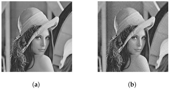
Figure 3. Original $512\times 512$ Lena image and its approximated low-rank image with rank 50. (a) Original Lena image. (b) Low-rank Lena image with rank 50.

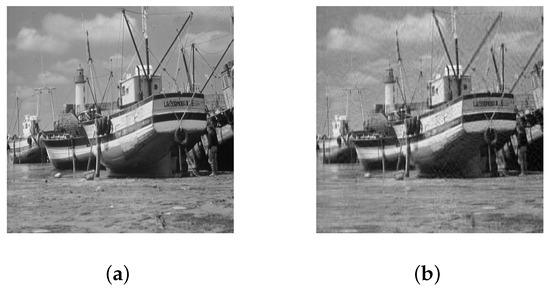
Figure 4. Original $512\times 512$ Boat image and its approximated low-rank image with rank 50. (a) Original Boat image. (b) Low-rank Boat image with rank 50.

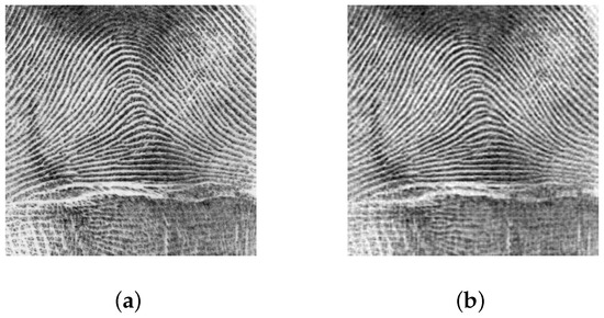
Figure 5. Original $512\times 512$ Fingerprint image and its approximated low-rank image with rank 50. (a) Original Fingerprint image. (b) Low-rank Fingerprint image with rank 50.

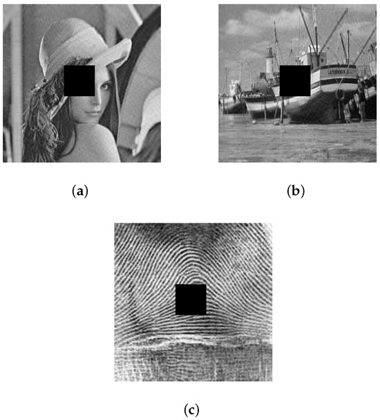
Figure 6. Low-rank images with 3.81% pixels missing. (a) 3.81% pixels missing Lena image. (b) 3.81% pixels missing Boat image. (c) 3.81% pixels missing Fingerprint image.

Table 1 reports the numerical results of the algorithms for image inpainting problems. For AIMDT algorithm, three different c values are considered, that is, $c=1,5,100$. From Table 1, we can make the following observations: (i) AIMDT algorithms with parameter $c=1,5,100$ are all superior to SVT algorithm in RE. In particular, the REs generated by the AIMDT algorithms decreases as the parameter c decreases; (ii) AIMDT algorithms with parameter $c=1,5,100$ are all more time-consuming than SVT algorithm. The calculation time of AIMDT algorithm increases with the decrease of parameter c. In a word, AIMDT algorithms can more accurately recover the low-rank grayscale images than SVT algorithm, and the AIMDT algorithm with parameter $c=1$ performs best. We display the recovered low-rank Lena, Boat and Fingerprint images in Figure 7, Figure 8 and Figure 9, respectively. From these figures, we can see that the AIMDT algorithm with parameter $c=1$ has the best performance in recovering the low-rank grayscale images.

Table 1. Numerical results of algorithms for image inpainting problems.

Image	AIMDT, $\mathit{c}=1$		AIMDT, $\mathit{c}=5$		AIMDT, $\mathit{c}=100$		SVT Algorithm
(Name, Rank, FR)	RE	Time	RE	Time	RE	Time	RE	Time
(Lena, 50, 5.17)	2.11 × 10−2	226.32	5.71 × 10−2	76.36	6.67 × 10−2	28.45	7.29 × 10−2	21.54
(Boat, 50, 5.17)	3.28 × 10−5	773.77	6.23 × 10−2	107.11	8.18 × 10−2	19.54	8.84 × 10−2	15.30
(Fingerprint, 50, 5.17)	4.21 × 10−6	94.00	1.34 × 10−2	67.86	5.68 × 10−2	10.03	6.29 × 10−2	8.03

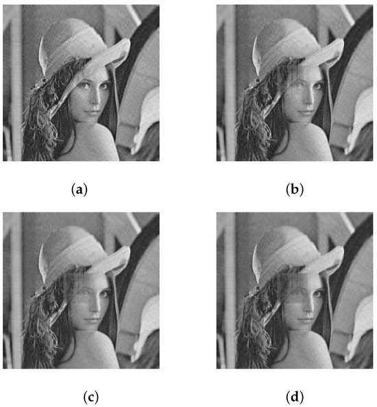
Figure 7. Comparisons of algorithms for recovering the low-rank Lena image with 3.81% pixels missing. (a) AIMDT algorithm, $c=1$. (b) AIMDT algorithm, $c=5$. (c) AIMDT algorithm, $c=100$. (d) SVT algorithm.

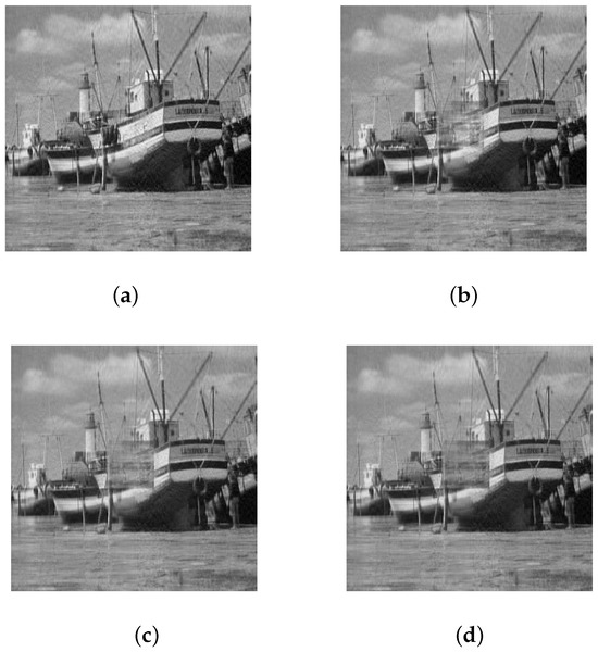
Figure 8. Comparisons of algorithms for recovering the low-rank Boat image with 3.81% pixels missing. (a) AIMDT algorithm, $c=1$. (b) AIMDT algorithm, $c=5$. (c) AIMDT algorithm, $c=100$. (d) SVT algorithm.

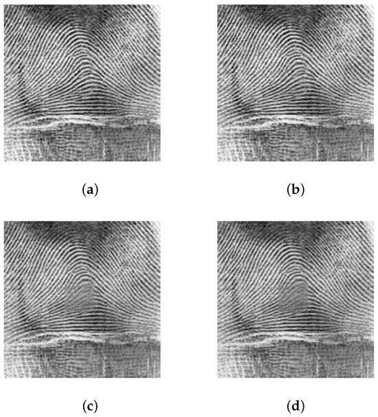
Figure 9. Comparisons of algorithms for recovering the low-rank Fingerprint image with 3.81% pixels missing. (a) AIMDT algorithm, $c=1$. (b) AIMDT algorithm, $c=5$. (c) AIMDT algorithm, $c=100$. (d) SVT algorithm.

5. Conclusions

In this paper, based on the designed thresholding operator which has less bias to the larger singular values than the soft thresholding operator, an iterative matrix designed thresholding algorithm and its adaptive version are proposed to recover the low-rank matrices. Numerical experiments on some image inpainting problems show that the adaptive iterative matrix designed thresholding algorithm performs efficiently in recovering the low-rank matrices. In the future work, we shall study the acceleration techniques to improve the convergence rate of the proposed algorithm and explore other applications for the designed thresholding operator.

References

- Candès, E.J.; Recht, B. Exact matrix completion via convex optimization. Found. Comput. Math. 2009, 9, 717–772. [Google Scholar] [CrossRef]
- Cao, F.; Cai, M.; Tan, Y. Image interpolation via low-rank matrix completion and recovery. IEEE Trans. Circuits Syst. Video Technol. 2015, 25, 1261–1270. [Google Scholar]
- Liu, Z.; Vandenberghe, L. Interior-point method for nuclear norm approximation with application to system identification. SIAM J. Matrix Anal. Appl. 2009, 31, 1235–1256. [Google Scholar] [CrossRef]
- Chen, P.; Suter, D. Recovering the missing components in a large noisy low-rank matrix: Application to SFM. IEEE Trans. Pattern Anal. Mach. Intell. 2004, 26, 1051–1063. [Google Scholar] [CrossRef] [PubMed]
- Xing, Z.; Zhou, J.; Ge, Z.; Huang, G.; Hu, M. Recovery of high order statistics of PSK signals based on low-rank matrix completion. IEEE Access 2023, 11, 12973–12986. [Google Scholar] [CrossRef]
- Tsakiris, M.C. Low-rank matrix completion theory via Plücker coordinates. IEEE Trans. Pattern Anal. Mach. Intell. 2023, 45, 10084–10099. [Google Scholar] [CrossRef] [PubMed]
- Wang, K.; Chen, Z.; Ying, S.; Xu, X. Low-rank matrix completion via QR-based retraction on manifolds. Mathematics 2023, 11, 1155. [Google Scholar] [CrossRef]
- Cai, J.-F.; Candès, E.J.; Shen, Z. A singular value thresholding algorithm for matrix completion. SIAM J. Optim. 2010, 20, 1956–1982. [Google Scholar] [CrossRef]
- Ma, S.; Goldfarb, D.; Chen, L. Fixed point and Bregman iterative methods for matrix rank minimization. Math. Program. 2011, 128, 321–353. [Google Scholar] [CrossRef]
- Recht, B.; Fazel, M.; Parrilo, P.A. Guaranteed minimum-rank solution of linear matrix equations via nuclear norm minimization. SIAM Rev. 2010, 52, 471–501. [Google Scholar] [CrossRef]
- Candès, E.J.; Tao, T. The power of convex relaxation: Near-optimal matrix completion. IEEE Trans. Inf. Theory 2010, 56, 2053–2080. [Google Scholar] [CrossRef]
- Sturm, J.F. Using SeDuMi 1.02, a MATLAB toolbox for optimization over symmetric cones. Optim. Methods Softw. 1999, 11, 625–653. [Google Scholar] [CrossRef]
- Tütüncü, R.H.; Toh, K.C.; Todd, M.J. Solving semidefinite-quadratic-linear programs using SDPT3. Math. Program. 2003, 95, 189–217. [Google Scholar] [CrossRef]
- Toh, K.-C.; Yun, S. An accelerated proximal gradient algorithm for nuclear norm regularized linear least squares problems. Pac. J. Optim. 2010, 6, 615–640. [Google Scholar]
- Yang, J.; Yuan, X. Linearized augmented lagrangian and alternating direction methods for nuclear norm minimization. Math. Comput. 2013, 82, 301–329. [Google Scholar] [CrossRef]
- Daubechies, I.; Defrise, M.; Mol, C.D. An iterative thresholding algorithm for linear inverse problems with a sparsity constraint. Commun. Pure Appl. Math. 2004, 57, 1413–1457. [Google Scholar] [CrossRef]
- Chartrand, R. Shrinkage mappings and their induced penalty functions. In Proceedings of the 2014 IEEE International Conference on Acoustics, Speech and Signal Processing (ICASSP), Florence, Italy, 4–9 May 2014. [Google Scholar]
- Peng, D.; Xiu, N.; Yu, J. S1/2 regularization methods and fixed point algorithms for affine rank minimization problems. Comput. Optim. Appl. 2017, 67, 543–569. [Google Scholar] [CrossRef]
- Xu, Z.; Chang, X.; Xu, F.; Zhang, H. L1/2 regularization: A thresholding representation theory and a fast solver. IEEE Trans. Neural Netw. Learn. Syst. 2012, 23, 1013–1027. [Google Scholar] [PubMed]
Disclaimer/Publisher’s Note: The statements, opinions and data contained in all publications are solely those of the individual author(s) and contributor(s) and not of MDPI and/or the editor(s). MDPI and/or the editor(s) disclaim responsibility for any injury to people or property resulting from any ideas, methods, instructions or products referred to in the content. |
© 2024 by the authors. Licensee MDPI, Basel, Switzerland. This article is an open access article distributed under the terms and conditions of the Creative Commons Attribution (CC BY) license (https://creativecommons.org/licenses/by/4.0/).