Golden Laplacian Graphs

Abstract

Many properties of the structure and dynamics of complex networks derive from the characteristics of the spectrum of the associated Laplacian matrix, specifically from the set of its eigenvalues. In this paper, we show that there exist graphs for which the ratio between the length of the spectrum (that is, the difference between the largest and smallest eigenvalues of the Laplacian matrix) and its spread (the difference between the second smallest eigenvalue and the smallest one) is equal to the golden ratio. We call such graphs Golden Laplacian Graphs (GLG). In this paper, we first find all such graphs with a number of nodes $n\le 10$. We then prove several graph-theoretic and algebraic properties that characterize these graphs. These graphs prove to be extremely robust, as they have large vertex and edge connectivity along with a large isoperimetric constant. Finally, we study the synchronization properties of GLGs, showing that they are among the top synchronizable graphs of the same size. Therefore, GLGs represent very good candidates for engineering and communication networks.

1. Introduction

Algebraic graph theory [1,2] plays an important role in the study of complex systems [3]. In particular, the study of the algebraic properties of the graph Laplacian matrix L is fundamental to understanding both the structure and the dynamics of networks. On the one hand, the eigenvalues of L are related to the robustness of a network against random failures and intentional attacks via the algebraic connectivity [4] and isoperimetric constant [5] of the graph. On the other hand, the same eigenvalues are directly related to the rate of convergence of diffusive models on networks [6] as well as their synchronizability [7] and electric resistance properties [8]. Thus, it is not rare to see efforts directed towards the computational optimization of Laplacian eigenvalues in order to improve the robustness and dynamical properties of real-world networked systems [9,10,11].

Here, we conduct a different approach to find graphs with special Laplacian spectral properties. In particular, we designate the spectrum of the graph Laplacian of G by $Sp\left(L\left(G\right)\right)=\left\{{\mu }_i^{{\omega }_i},i=1\dots ,n\right\}$, where ${\mu }_i$ is an eigenvalue of L and ${\omega }_i$ is its multiplicity. We order the eigenvalues of L as $0={\mu }_1<{\mu }_2\le \cdots \le {\mu }_n$; then, we look for the existence of graphs for which

$${\displaystyle \frac{{\mu }_n-{\mu }_1}{{\mu }_n-{\mu }_2}}={\displaystyle \frac{{\mu }_n-{\mu }_2}{{\mu }_2-{\mu }_1}}=\phi ,$$

(1)

where $\phi =\left(1+\sqrt{5}\right)/2$ is the “golden ratio”. It has been claimed that the golden ratio is ubiquitous in nature [12]; thus, it is interesting to know whether such a number can appear in the ratio of important eigenvalues of the graph Laplacian. We prove here that such graphs, called Golden Laplacian Graphs (GLG) hereinafter, exist. While similar spectral relations for the adjacency matrix of graphs were previously studied in [13,14], this is the first time the question has been asked in terms of the Laplacian matrix of a graph. We prove a few structural properties of GLGs, showing that they are small-world [15], in the sense of having a very small diameter, robust to vertex and edge removal, and have a large isopermetric constant. In addition, we prove a few bounds for different structural parameters of these graphs. We prove that the smallest GLG is the cycle with five vertices and that there are no other GLGs with fewer than eight vertices. We find all GLGs with $n=8,9,10$ vertices and obtained a few of their structural properties, showing that they all have a diameter equal to 2, are Hamiltonian, and have perfect (for an even number of vertices) or nearly-perfect (for an odd number of vertices) matching, among other interesting properties. Moreover, GLGs are shown to be among the best synchronizable graphs of the same size. For instance, GLGs are in the top 3.32% for best synchronizability among eight-vertex graphs, the top $2.52\%$ for $n=9$, and the top $1.64\%$ for $n=10.$ As we have proved here, GLGs can be expanded to larger sizes using specific matrix operations. Therefore, these robust and highly synchronizable graphs are good candidates for networks in the application areas of engineering and communication systems.

2. Preliminaries

Let $G=\left(V,E\right)$ be a simple connected graph and let $L=K-A$ be its Laplacian matrix, where K is the diagonal matrix of the vertex degree and A is its adjacency matrix. Let $0={\mu }_1<{\mu }_2\le \cdots \le {\mu }_n$ be the eigenvalues of the Laplacian matrix of G. We call ${\mu }_n$ the length of the Laplacian spectrum and ${\mu }_2$ the algebraic connectivity of G.

The following are standard definitions in graph theory which we use in this paper, in which we follow [16].

The distance between two vertices in G is the length (number of edges) of the shortest path connecting the two vertices. The diameter D is the maximum of all distances between pairs of vertices in G.

A vertex subset is an independent set if no two of its vertices are adjacent. The largest cardinality of an independent set in G is the independence number, $ind\left(G\right)$.

A graph is Hamiltonian if it contains a spanning cycle (Hamiltonian cycle). The graph is Hamiltonian connected if any pair of vertices are the ends of a spanning path.

A graph of order n is pancyclic if it contains cycles of all length l, $3\le l\le n$. Obviously, a pancyclic graph is Hamiltonian.

The vertex connectivity of a connected graph ${\kappa }_v\left(G\right)$ is the minimum number of vertices for which their removal either disconnects G or reduces it to a single-vertex graph. A graph is k-connected if ${\kappa }_v\left(G\right)\ge k$.

The clique number $\omega \left(G\right)$ is the number of vertices in a largest clique of G.

A matching in G is a set of mutually non-adjacent edges in G. A matching is perfect if every vertex in G is incident to some edge in the matching. If the number of vertices of G is odd, the graph may contain a near-perfect matching if exactly one vertex is unmatched.

A set $S\subseteq V$ is a dominating set of a graph G if each vertex in V is in S or is adjacent to a vertex in S. The domination number $\gamma \left(G\right)$ is the minimum cardinality of a dominating set of G.

The isopermetric number of a graph is defined as follows. Let $S\subset V$ and let $\partial S$ be the edge boundary of S, i.e., those edges with one endpoint inside S and another outside S. Then, the isopermetric number is

$$h\left(G\right)=\underset{1\le \left|S\right|\le \frac{n}{2}}{min}{\displaystyle \frac{\left|\partial S\right|}{\left|S\right|}}.$$

(2)

We now introduce several classes of graphs which are used in this work. Note that different notations are used in the literature for certain classes.

Path graph on n vertices, $P_n$: the graph with $n-2$ vertices of degree two and two vertices of degree one.

Cycle graph on n vertices, $C_n$: the graph with n vertices of degree two.

Complete graph on n vertices, $K_n$: the graph with all vertices of degree $n-1$.

Complete graph minus an edge, $K_n-e$: the complete graph $K_n$ on which an edge has been deleted.

Complete bipartite graph on n vertices, $K_{p,q}$: the graph on $n=p+q$ vertices which can be partitioned into two subsets of cardinalities p and q, respectively, such that no edge has both endpoints in the same subset and every possible edge that could connect vertices in different subsets is part of the graph.

Complete split graph on n vertices, $S_{n,\alpha }$: the graph on n vertices consisting of a clique on $n-\alpha$ vertices and an independent set on the remaining $\alpha$ ($1\le \alpha \le n-1$) vertices in which each vertex of the clique is adjacent to each vertex of the independent set.

Lollipop graph on n vertices, $H_{n,p}$: the graph on n vertices obtained by appending a cycle $C_p$ to a pendant vertex of a path $P_{n-p}$.

Kite graph on n vertices, $Y_{p,q}$: the graph on $n=p+q$ vertices obtained by appending a complete graph $K_p$ to a pendant vertex of a path $P_q$.

Friendship graph on n vertices, $F_r$: the graph on $n=2r+1$ vertices consisting of r triangles attached to a common vertex.

Wheel graph on n vertices, $W_n$: the graph on n vertices obtained by the graph join operation $C_{n-1}+K_1$, which consists of connecting every vertex of a cycle $C_{n-1}$ to a common vertex not in the cycle.

Fan graph on n vertices, $A_n$: the graph on n vertices resulting from the graph join operation $P_{n-1}+K_1$, consisting of joining every vertex of a path graph $P_{n-1}$ to a single vertex not in the cycle; we propose using the letter A from the Spanish “abanico”, meaning “fan”.

Let $G_1$ and $G_2$ be two graphs of orders $n_1$ and $n_2$ with the corresponding adjacency matrices $A_1$ and $A_2$. Then, the Kronecker (or tensor) product $G_1\otimes G_2$ is the graph with the adjacency matrix provided by

$$A_1\otimes A_2\left[\begin{array}{ccc}{a}_{11}{A}_2& \dots & A_2\\ ⋮& \ddots & ⋮\\ a_{n_{1}1}{A}_2& \dots & a_{n_1{n}_1}{A}_2\end{array}\right].$$

(3)

For general properties of the Kronecker product, we direct the reader to [17,18].

3. Golden Laplacian Spectra

We start by associating a line segment of length ${\mu }_n$ with the spectrum of L, which is due to the fact that ${\mu }_1=0$. We then divide the segment into two sections of lengths ${\mu }_n-{\mu }_2$ (the largest section) and ${\mu }_2$ (the shortest section), as illustrated in Figure 1.

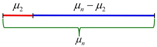
Figure 1. Representation of the spectrum of the Laplacian matrix of a graph as a segment of line.

Then, we have the following.

Definition 1.

A graph G for which

$${\displaystyle \frac{{\mu }_n}{{\mu }_n-{\mu }_2}}={\displaystyle \frac{{\mu }_n-{\mu }_2}{{\mu }_2}}=\phi ,$$

(4)

where $\phi ={\displaystyle \frac{\sqrt{5}+1}{2}}$ is the golden ratio, is called a Golden Laplacian Graph (GLG).

It is clear that (4) accounts for the ratio of the whole to the largest section (${\displaystyle \frac{{\mu }_n}{{\mu }_n-{\mu }_2}}$) and the ratio of the largest section to the smallest section $({\displaystyle \frac{{\mu }_n-{\mu }_2}{{\mu }_2}})$. It is well known that both ratios are equal only when they are exactly equal to the golden ratio. In a GLG, we have

$$\mathcal{Q}\left(G\right){\displaystyle \frac{{\mu }_n}{{\mu }_2}}=\phi +1={\phi }^2,$$

(5)

where $\mathcal{Q}\left(G\right)=\mathcal{Q}$ is the well-known eigenratio of the graph. The importance of this parameter resides in the role it plays in the synchronization of networks [7,10,11,19,20]. Smaller values of $\mathcal{Q}$ favor the synchronizability of the graph. The smallest possible value of $\mathcal{Q}$ is attained for the complete graph $K_n$, $\mathcal{Q}\left(K_n\right)=1$, which displays the best possible synchronizability for graphs with n vertices and which is also the densest one.

Properties of GLGs

Next, we study some properties of GLGs. We first state some general results for ${\mu }_n$ and ${\mu }_2$ which are used in the proofs of several of the results obtained herein (see also Chapter 6 in [21] and references therein). Other more specific properties are stated when used.

Lemma 1.

Let G be a graph with maximum and minimum degrees Δ and δ, respectively; then:

• $\Delta +1\le {\mu }_n\le n$. The left inequality holds if $\Delta =n-1$ and the right one if and only if the complement of G is disconnected (see [22,23]);
• ${\mu }_n\left(G_n\right)\le max\left\{{\displaystyle \frac{k_u\left(k_u+m_u\right)+k_v\left(k_v+m_v\right)}{k_u+k_v}},u,v\in E\right\}$, where $m_u$ is the average degree of the nearest neighbors of the vertex u (see [24]);
• ${\mu }_2\le {\displaystyle \frac{n-1}{n}}\delta$ (see [25]);
• ${\mu }_2\le c_v\le c_e\le \delta$, where $c_v$ and $c_e$ denote the vertex and edge connectivity, respectively (see [25]).

We now start to prove some of the properties of GLGs.

Lemma 2.

Let G be a GLG with n vertices, m edges, and an edge density equal to $d=\frac{2m}{n\left(n-1\right)}$. Then,

$${\displaystyle \frac{\Delta +1}{{\phi }^{2}n}}\le {\displaystyle \frac{{\mu }_n}{{\phi }^{2}n}}\le d\le {\displaystyle \frac{{\phi }^2{\mu }_2}{n}}\le {\displaystyle \frac{{\phi }^2\delta }{n}},$$

(6)

where δ and Δ are the minimum and maximum degrees, respectively.

Proof. 

Because $2m={\sum }_{j=1}^n{\mu }_j$, we have $2m\ge \left(n-1\right){\mu }_2$, from which we obtain

$$2m\ge {\displaystyle \frac{\left(n-1\right){\mu }_n}{{\phi }^2}}\ge {\displaystyle \frac{\left(n-1\right)\left(\Delta +1\right)}{{\phi }^2}},$$

(7)

and we can obtain the lower bound by dividing both sides by $n\left(n-1\right)$. In a similar way, we have $2m\le \left(n-1\right){\mu }_n$, from which we obtain

$$2m\le \left(n-1\right){\phi }^2{\mu }_2\le \left(n-1\right){\phi }^2\delta ,$$

(8)

which provides the final result by dividing both sides by $n\left(n-1\right)$. □

Lemma 3.

Let G be a GLG with minimum and maximum degrees $\delta =\delta \left(G\right)$ and $\Delta =\Delta \left(G\right)$, respectively. Then,

$${\displaystyle \frac{\Delta -\delta +1}{\delta }}\le \phi \le {\displaystyle \frac{n}{\Delta -\delta +1}}.$$

(9)

Proof. 

Using points 1 and 4 from Lemma 1, we have ${\mu }_2\le \delta$ and ${\mu }_n\ge \Delta +1$. Then, because in a GLG we have

$${\displaystyle \frac{{\mu }_n-{\mu }_2}{{\mu }_2}}=\phi ,$$

(10)

we have the lower bound. The upper bound is based on the fact that

$${\displaystyle \frac{{\mu }_n}{{\mu }_n-{\mu }_2}}=\phi$$

(11)

and ${\mu }_n\le n$ in a GLG, which when combined with ${\mu }_n-{\mu }_2\ge \Delta -\delta +1$, completes the result. □

The following results are elementary from the fact that ${\mu }_n/{\mu }_2={\phi }^2$ in a GLG.

Lemma 4.

Let G be a GLG with minimum and maximum degrees $\delta =\delta \left(G\right)$ and $\Delta =\Delta \left(G\right)$, respectively. Then,

$${\displaystyle \frac{\Delta +1}{\delta }}\le {\phi }^2.$$

(12)

Lemma 5.

Let G be a GLG with an average degree $\overline{k}={\displaystyle \frac{1}{n}}{\sum }_{i=1}^n{k}_i$. Then,

$${\displaystyle \frac{{\mu }_n}{{\phi }^2}}\le \overline{k}\le {\phi }^2{\mu }_2.$$

(13)

We now prove some results connecting the spectra of GLGs to some of their properties.

Lemma 6.

Let G be a GLG with n vertices and a maximum degree $\Delta =\Delta \left(G\right)$. Let $h\left(G\right)$ be the isoperimetric number of G. Then,

$${\displaystyle \frac{\Delta +1}{2{\phi }^2}}\le {\displaystyle \frac{{\mu }_n}{2{\phi }^2}}\le h\left(G\right)<\sqrt{{\displaystyle \frac{n\Delta }{\phi }}}.$$

(14)

Proof. 

The lower bound is proved by plugging into [5] the facts that (i) ${\mu }_2={\displaystyle \frac{{\mu }_n}{{\phi }^2}}$ in GLGs and (ii) that ${\mu }_n\ge \Delta +1$ [22], as follows:

$${\displaystyle \frac{{\mu }_2}{2}}\le h\left(G\right).$$

(15)

For the upper bound, we use the fact that for a graph different from the complete graphs $K_1$, $K_2$, and $K_3$, we have [5]

$$h\left(G\right)\le \sqrt{{\mu }_2\left(2\Delta -{\mu }_2\right)}.$$

(16)

Then, again using the fact that in a GLG we have ${\mu }_2={\displaystyle \frac{{\mu }_n}{{\phi }^2}}$ and ${\mu }_n\le n$,

$$h\left(G\right)\le \sqrt{{\mu }_2\left(2\Delta -{\mu }_2\right)}\le {\displaystyle \frac{\sqrt{n\left(2\Delta {\phi }^2-{\mu }_n\right)}}{{\phi }^2}},$$

(17)

and because ${\mu }_n\le \Delta +1<\Delta$, we obtain

$$h\left(G\right)<{\displaystyle \frac{\sqrt{n\Delta \left(2{\phi }^2-1\right)}}{{\phi }^2}}.$$

(18)

Finally, using the fact that $2\phi +1={\phi }^4$, we have ${\displaystyle \frac{2{\phi }^2-1}{{\phi }^4}}=\phi -1={\phi }^{-1}$, proving the result. □

Lemma 7.

Let X and Y be disjoint sets of vertices of an GLG such that there is no edge between X and Y. Then,

$${\displaystyle \frac{\left|X\right|\left|Y\right|}{n\left(n-\left|X\right|-\left|Y\right|\right)}}\le {\displaystyle \frac{1}{5}}.$$

(19)

Proof. 

It has been proved (see Proposition 4.8.1 in [26]) that

$${\displaystyle \frac{\left|X\right|\left|Y\right|}{\left(n-\left|X\right|\right)\left(n-\left|Y\right|\right)}}\le {\left({\displaystyle \frac{{\mu }_n-{\mu }_2}{{\mu }_n+{\mu }_2}}\right)}^2.$$

(20)

Because the graph is a GLG, we then have

$${\left({\displaystyle \frac{{\mu }_n-{\mu }_2}{{\mu }_n+{\mu }_2}}\right)}^2={\left({\displaystyle \frac{{\phi }^2-1}{{\phi }^2+1}}\right)}^2={\left({\displaystyle \frac{\phi }{\phi +2}}\right)}^2={\displaystyle \frac{1}{5}}.$$

(21)

□

Lemma 8.

Let G be a GLG with n vertices and diameter D; then,

$$D\le 2⌈{\displaystyle \frac{{\phi }^2+1}{4}}ln\left(n-1\right)⌉<2⌈ln\left(n-1\right)⌉.$$

(22)

Proof. 

Mohar [27] has proved that

$$D\le 2⌈{\displaystyle \frac{\Delta +{\mu }_2}{4{\mu }_2}}ln\left(n-1\right)⌉.$$

(23)

Then, because ${\mu }_n\ge \Delta$, we have

$$D\le 2⌈{\displaystyle \frac{{\mu }_n+{\mu }_2}{4{\mu }_2}}ln\left(n-1\right)⌉,$$

(24)

from which the first inequality follows for a GLG where ${\displaystyle \frac{{\mu }_n}{{\mu }_2}}={\phi }^2$. The second inequality comes from the fact that ${\displaystyle \frac{{\phi }^2+1}{4}}={\displaystyle \frac{\sqrt{5}+5}{8}}<1.$ □

Lemma 9.

Let G be a GLG with n vertices and diameter D; then,

$$D\le 1+⌊{\displaystyle \frac{{cosh}^{-1}\left(n-1\right)}{{cosh}^{-1}\sqrt{5}}}⌋.$$

(25)

Proof. 

Chung et al. [28] have proved that

$$D\le 1+⌊{\displaystyle \frac{{cosh}^{-1}\left(n-1\right)}{{cosh}^{-1}\left({\displaystyle \frac{{\mu }_n+{\mu }_2}{{\mu }_n-{\mu }_2}}\right)}}⌋.$$

(26)

Thus, in a GLG we have ${\mu }_n\pm {\mu }_2={\phi }^2{\mu }_2\pm {\mu }_2$, from which the result is straightforward using the properties of $\phi .$ □

Remark 1.

Notice that when using Lemma 9, any GLG with $n\le 9$ necessarily has diameter smaller or equal than 2. Because $\mathcal{Q}\left(K_n\right)=1$, which is the only graph with diameter 1, this means that a GLG with $n\le 9$ has a diameter equal to 2.

Lemma 10.

Let G be a GLG of size n with independence number $ind\left(G\right).$ Then, if G has minimum and maximum degrees provided by δ and Δ, respectively,

$$ind\left(G\right)\le {\displaystyle \frac{n\delta }{\phi {\mu }_2}}={\displaystyle \frac{\phi n\delta }{{\mu }_n}}\le {\displaystyle \frac{\phi n\delta }{\Delta +1}}.$$

(27)

Proof. 

Here, we use a result of Lu et al. [29], who proved that

$$ind\left(G\right)\le {\displaystyle \frac{n\left({\mu }_n-\delta \right)}{{\mu }_n}}.$$

(28)

Using the fact that for a GLG we have ${\mu }_n={\phi }^2{\mu }_2$ and ${\mu }_2\le \delta$, we can state the following theorem.

Theorem 1.

Because we have

$$ind\left(G\right)\le {\displaystyle \frac{n\left({\phi }^2\delta -\delta \right)}{{\phi }^2{\mu }_2}}={\displaystyle \frac{n\delta }{\phi {\mu }_2}},$$

(29)

we can use ${\mu }_2={\displaystyle \frac{{\mu }_n}{{\phi }^2}}$ and the fact that ${\mu }_n\ge \Delta +1$ to obtain the last inequality.

□

Lemma 11.

Let G be a GLG of size n with matching number $\alpha \left(G\right)$; then,

$$\alpha \left(G\right)\ge ⌈{\displaystyle \frac{n-1}{{\phi }^2}}⌉.$$

(30)

Proof. 

Here, we use a result of Gu and Liu [30], who proved that

$$\alpha \left(G\right)\ge min\left\{⌈{\displaystyle \frac{{\mu }_2}{{\mu }_n}}\left(n-1\right)⌉,⌈{\displaystyle \frac{1}{2}}\left(n-1\right)⌉\right\}.$$

(31)

Because in a GLG we have ${\displaystyle \frac{{\mu }_2}{{\mu }_n}}={\displaystyle \frac{1}{{\phi }^2}}<{\displaystyle \frac{1}{2}}$, we obtain the result. □

4. Discovering GLGs

In this section, we state several results, which allow us to discover GLGs. We start by proving results concerning the nonexistence of GLGs in certain classes of graphs. While the following result is trivial, we state it here as it is used in several of the following results.

Lemma 12.

Let $G_n$ be a finite graph such that ${\mu }_n\left(G_n\right)\in \mathbb{N}$ and ${\mu }_2\left(G_n\right)\in \mathbb{N}$; then, $G_n$ is not a GLG.

Proof. 

The proof follows immediately from the fact that in a GLG we have ${\mu }_n/{\mu }_2={\phi }^2=\phi +1$. Because $\phi$ is irrational, as is ${\phi }^2$, it cannot be expressed as the ratio of two integers. □

Lemma 13.

Let $G_n$ be a graph such that $G_n\in \left\{P_n,K_n,K_{p,q},S_{n,\alpha },H_{n,p},Y_{p,q},K_n-e,F_r,W_n,A_n\right\}$; then, $G_n$ is not a GLG.

Proof. 

(a) Let $G_n$ be isomorphic to $P_n$; then,

$$Sp\left(L\left(P_n\right)\right)=\left\{2\left(1-cos{\displaystyle \frac{j\pi }{n}}\right),j=1,\dots ,n\right\}.$$

(32)

Therefore, the eigenratio of $P_n$ is

$$\mathcal{Q}\left(P_n\right)={\displaystyle \frac{1-cos{\displaystyle \frac{\left(n-1\right)\pi }{n}}}{1-cos{\displaystyle \frac{\pi }{n}}}}={cot}^2\left({\displaystyle \frac{\pi }{2n}}\right),$$

(33)

which is different from ${\phi }^2$ for any $n\in \mathbb{N}$.

(b) Let $G_n$ be isomorphic to $K_n.$ Because $Sp\left(L\left(K_n\right)\right)=\left\{n^{n-1},0\right\}$, we have $\mathcal{Q}\left(K_n\right)=1$.

(c) Let $G_n$ be isomorphic to $K_{p,q}$ with $p\ge q$; then,

$$Sp\left(L\left(K_{p,q}\right)\right)=\left\{p+q,p^{q-1},q^{p-1},0\right\}.$$

(34)

Therefore,

$$\mathcal{Q}\left(K_{p,q}\right)={\displaystyle \frac{p+q}{q}},$$

(35)

which is a rational number, and consequently different from ${\phi }^2.$

(d) Let $G_n$ be isomorphic to $S_{n,\alpha }$; then,

$$Sp\left(L\left(S_{n,\alpha }\right)\right)=\left\{n^{n-\alpha },{\left(n-\alpha \right)}^{\alpha -1},0\right\}.$$

(36)

Therefore,

$$\mathcal{Q}\left(S_{n,\alpha }\right)={\displaystyle \frac{n}{n-\alpha }},$$

(37)

which is a rational number, and consequently different from ${\phi }^2.$

(e) Let $G_n$ be isomorphic to $H_{n,p}$. Then, using the bound from point 2 of Lemma 1, we have $4\le {\mu }_n\left(H_{n,p}\right)\le 4.8$. In addition, because ${\mu }_2\left(G_n\right)\le \delta$ for any graph, we have ${\mu }_2\left(H_{n,p}\right)\le 1$ (because it always has a pendant vertex), which implies that $\mathcal{Q}\left(H_{n,p}\right)\ge 4$.

(f) Let $G_n$ be isomorphic to $Y_{p,q}$. Because ${\mu }_n\left(G_n\right)=n$ in any graph if and only if $\Delta =n-1$ (see point 1 from Lemma 1), we have ${\mu }_n\left(Y_{p,q}\right)=n$. In addition, ${\mu }_2\left(Y_{p,q}\right)\le 1$, as there is always a pendant vertex, which implies that $\mathcal{Q}\left(Y_{p,q}\right)\ge n$, which is different from ${\phi }^2$ for $n\ge 3$. For $n\le 2$, the kite graph is isomorphic to $K_n,$ which has already been proved to not be a GLG.

(g) Let $G_n$ be isomorphic to $K_n-e$; then,

$$Sp\left(L\left(K_n-e\right)\right)=\left\{n^{n-2},n-2,0\right\},$$

(38)

which implies that

$$\mathcal{Q}\left(K_n-e\right)={\displaystyle \frac{n}{n-2}},$$

(39)

which is a rational number and consequently different from ${\phi }^2.$

(h) Let $G_n$ be isomorphic to $F_r$; then,

$$Sp\left(L\left(F_r\right)\right)=\left\{2r+1,3^r,1^{r-1},0\right\},$$

(40)

which implies that

$$\mathcal{Q}\left(F_r\right)=2r+1,$$

(41)

which is an integer number, therefore different from ${\phi }^2.$

(i) Let $G_n$ be isomorphic to $W_n$. Then,

$$Sp\left(L\left(W_n\right)\right)=\left\{n,3-2cos{\displaystyle \frac{2j\pi }{n}},j=1,\dots ,n-1\right\}.$$

(42)

Therefore,

$$\mathcal{Q}\left(W_n\right)={\displaystyle \frac{n}{5-4{cos}^2\left({\displaystyle \frac{\pi }{n-1}}\right)}},$$

(43)

which is different from ${\phi }^2$ for any $n\in \mathbb{N}$.

(j) Let $G_n$ be isomorphic to $A_n$. Then, because ${\mu }_n\left(G_n\right)=n$ in any graph if and only if $\Delta =n-1$ (see point 1 from Lemma 1), we have ${\mu }_n\left(A_n\right)=n$. In addition, from the definition of the graph we have ${\mu }_2\left(A_n\right)\le \delta =2$, which implies that $\mathcal{Q}\left(A_n\right)\ge {\displaystyle \frac{n}{2}}.$ Then, for $n\ge 6$ we have $\mathcal{Q}\left(A_n\right)>{\phi }^2$. The fan graph with four vertices is isomorphic to the complete split graph $S_{4,2}$. The fan graph with three vertices is isomorphic to $K_3$. Both graphs have been proved to not be GLGs. The remaining graph is $A_5$. The algebraic connectivity of this graph is ${\mu }_2\left(A_5\right)\approx 1.5858$, which implies that $\mathcal{Q}\left(A_5\right)>{\phi }^2$. Thus, no $A_n$ is a GLG. □

We now prove that no tree is a GLG, for which we use the following auxiliary result.

Lemma 14.

Let $T_n$ be a tree with n vertices; then, $T_n$ is not a GLG.

Proof. 

Let $T_n$ be a tree with $n>2$; then, $\delta \left(T_n\right)=1$ (because there is at least two pendant vertices) and $\Delta \left(T_n\right)\ge 2$ (because $n>2$). Therefore, using points 1 and 4 from Lemma 1, we have ${\mu }_n\left(T_n\right)\ge \Delta \left(T_n\right)+1\ge 3$ and ${\mu }_2\left(T_n\right)\le \delta \left(T_n\right)\le 1$ such that

$$\mathcal{Q}\left(T_n\right)={\displaystyle \frac{{\mu }_n\left(T_n\right)}{{\mu }_2\left(T_n\right)}}\ge 3>{\phi }^2.$$

(44)

For $n\le 2$, the existing trees are complete graphs with one and two vertices, which have already been proved to not be GLGs, which proves the result. □

Lemma 15.

Let $G_n$ be isomorphic to $C_n$. Then, $G_n$ is a GLG if and only if $n=5.$

Proof. 

The Laplacian eigenvalues of $C_n$ are

$$Sp\left(L\left(C_n\right)\right)=\left\{2-2cos{\displaystyle \frac{2j\pi }{n}},j=0,\dots ,n-1\right\}.$$

(45)

Therefore, for even n,

$$\mathcal{Q}\left(C_n\right)={\displaystyle \frac{2}{2-2{cos}^2\left({\displaystyle \frac{\pi }{n}}\right)}}n \mathrm{even},$$

(46)

which is different from ${\phi }^2$ for any $n\in \mathbb{N}$.

For odd n,

$$\mathcal{Q}\left(C_n\right)={\displaystyle \frac{1-cos\left({\displaystyle \frac{\left(n-1\right)\pi }{n}}\right)}{1-cos\left({\displaystyle \frac{2\pi }{n}}\right)}}n \mathrm{odd},$$

(47)

which is a monotonically increasing function and is exactly equal to ${\phi }^2$ only when $n=5$, in which case

$$\mathcal{Q}\left(C_5\right)={\displaystyle \frac{1-cos\left({\displaystyle \frac{4\pi }{5}}\right)}{1-cos\left({\displaystyle \frac{2\pi }{5}}\right)}}={\displaystyle \frac{3+\sqrt{5}}{2}}=\phi +1={\phi }^2.$$

(48)

□

Lemma 16.

The graph $C_5$ is the smallest GLG.

Proof. 

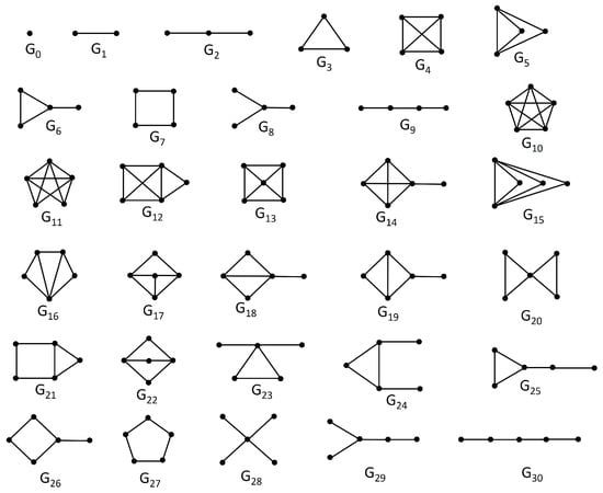
There are 31 connected graphs $G_n$ with $n\le 5$, which are illustrated in Figure 2. We can check the following: $G_1$, $G_2$, $G_8$, $G_9$, $G_{28}$, $G_{29}$, and $G_{30}$ are trees; $G_3$, $G_7$ and $G_{27}$ are cycles (which include $G_{27}=C_5$); $G_0$, $G_1$, $G_3$, $G_4$, and $G_{10}$, are complete graphs; $G_5$ and $G_{15}$ are complete split graphs; $G_6$, $G_{25}$, and $G_{26}$ are lollipop graphs; $G_{14}$ is a kite; $G_{11}$ is a complete graph minus an edge; $G_{20}$ is a friendship graph; $G_{13}$ is a wheel; $G_{16}$ is a fan graph; and $G_{22}$ is a complete bipartite graph. All of these except $C_5$ have been proved to not be GLGs.

Figure 2. The 31 connected graphs with $n\le 5$ vertices.

There are seven remaining graphs which we need to prove are not GLGs. The graphs $G_{12}$, $G_{17}$, $G_{18}$, and $G_{23}$ have integer Laplacian spectra: $Sp\left(L\left(G_{12}\right)\right)=\left\{5,5,4,2,0\right\}$; $Sp\left(L\left(G_{17}\right)\right)=\left\{5,4,3,2,0\right\}$; $Sp\left(L\left(G_{18}\right)\right)=\left\{5,4,2,1,0\right\}$; $Sp\left(L\left(G_{23}\right)\right)=\left\{5,3,1,1,0\right\}$, respectively. Thus, none of them can be GLGs, as proved in Lemma 12. The graphs $G_{19}$ and $G_{24}$ have $\Delta =3$ and $\delta =1$, such that ${\mu }_n\ge 4$ and ${\mu }_2\le 1$; consequently, $\mathcal{Q}\ge 4$ for these two graphs, meaning that they cannot be GLGs. The last graph remaining is $G_{21}$, which has ${\mu }_n\left(G_{21}\right)\approx 4.618$ and ${\mu }_2\left(G_{21}\right)\approx 1.382$, indicating that $\mathcal{Q}\left(G_{21}\right)>3>{\phi }^2.$ Therefore, $C_5$ is the only GLG with $n\le 5$, which proves the result. □

Next, we state a result which corresponds to the construction of GLGs with infinite size.

Lemma 17.

Let $K_{p,q}$ be a complete bipartite graph with $p>q$. If $p=F_{r+1}$ and $q=F_r$ or if $p=L_{r+1}$ and $q=L_r$, where $F_r$ and $L_r$ are the rth Fibonacci and Lucas numbers, respectively, then $K_{p,q}$ is GLG when $r\to \infty$.

Proof. 

It is known that ${\mu }_n\left(K_{p,q}\right)=p+q$ and ${\mu }_2\left(K_{p,q}\right)=q$. Thus, when $p=F_{r+1}$ and $q=F_r$ or when $p=L_{r+1}$ and $q=L_r$, we have

$$\mathcal{Q}\left(K_{F_{r+1},F_r}\right)={\displaystyle \frac{F_{r+1}}{F_r}}+1$$

(49)

or

$$\mathcal{Q}\left(K_{L_{r+1},L_r}\right)={\displaystyle \frac{L_{r+1}}{L_r}}+1.$$

(50)

Because [31]

$$\underset{r\to \infty }{lim}{\displaystyle \frac{F_{r+1}}{F_r}}=\underset{r\to \infty }{lim}{\displaystyle \frac{L_{r+1}}{L_r}}=\phi ,$$

(51)

we have ${\displaystyle \underset{r\to \infty }{lim}}\mathcal{Q}\left(K_{F_{r+1},F_r}\right)={\displaystyle \underset{r\to \infty }{lim}}\mathcal{Q}\left(K_{L_{r+1},L_r}\right)={\phi }^2$, as required for GLGs. □

Computer-Based Search

Here, we use an intensive computer search for detecting GLGs among the graphs with $6\le n\le 10$. For this, we calculated the ratio of the largest to smallest nontrivial eigenvalue of L for all connected graphs with $6\le n\le 10$. For each graph G, we used Matlab to check whether ${\mu }_n\left(G\right)/{\mu }_2\left(G\right)-{\phi }^2<{10}^{-10}$. For every one of the graphs fulfilling this condition, we used symbolic computation in Matlab to check whether it obeyed ${\mu }_n\left(G\right)/{\mu }_2\left(G\right)={\phi }^2$, with the following results:

• There are no GLGs among the 112 connected graphs with $n=6$ vertices;
• There are no GLGs among the 853 connected graphs with $n=7$ vertices;
• There are 15 GLGs among the 11,117 connected graphs with $n=8$ vertices (see Figure 3).
  

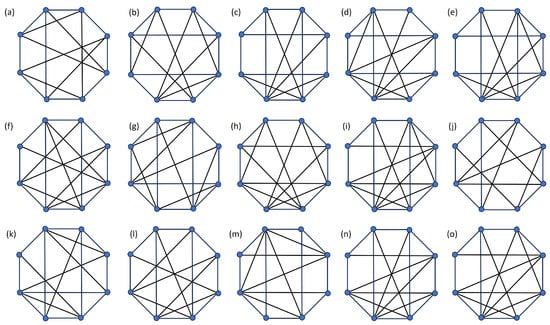  Figure 3. (a–o) Illustration of the 15 connected graphs with $n=8$ vertices which have golden Laplacian spectra.

In Table 1, we indicate some of the properties of these GLGs with eight vertices. The definitions of the terms are provided in Preliminaries section. Additionally, the terms H, P, M, r, and p respectively indicate whether the graphs are Hamiltonian, pancyclic, have a perfect matching, and are regular and planar, for which the responses yes (Y) or no (N) apply to their presence or absence, respectively.

Table 1. Properties of GLGs with $n=8$ vertices.

#	m	$\mathit{\delta }$	$\Delta$	D	ind	${\mathit{\kappa }}_{\mathit{v}}$	${\mathit{\kappa }}_{\mathit{e}}$	$\mathit{\omega }$	$\mathit{\gamma }$	H	P	M	r	p
a	16	4	4	2	3	4	4	3	2	Y	Y	Y	Y	N
b	17	4	5	2	3	4	4	4	2	Y	Y	Y	N	N
c	17	3	6	2	3	3	3	4	2	Y	Y	Y	N	N
d	18	3	6	2	3	3	3	4	2	Y	Y	Y	N	N
e	18	3	6	2	3	3	3	4	2	Y	Y	Y	N	N
f	18	3	5	2	3	3	3	4	2	Y	Y	Y	N	N
g	18	4	5	2	2	4	4	3	2	Y	Y	Y	N	Y
h	18	4	5	2	2	4	4	4	2	Y	Y	Y	N	N
i	19	3	6	2	2	3	3	4	2	Y	Y	Y	N	N
j	16	3	5	2	3	3	3	3	2	Y	Y	Y	N	N
k	17	3	5	2	3	3	3	3	2	Y	Y	Y	N	N
l	17	3	5	2	3	3	3	3	2	Y	Y	Y	N	N
m	18	3	6	2	4	3	3	4	2	Y	Y	Y	N	Y
n	18	3	6	2	3	3	3	4	2	Y	Y	Y	N	N
o	18	3	6	2	3	3	3	4	2	Y	Y	Y	N	N

• There are five GLGs among the 261,080 connected graphs with $n=9$ vertices, which are illustrated in Figure 4.
  

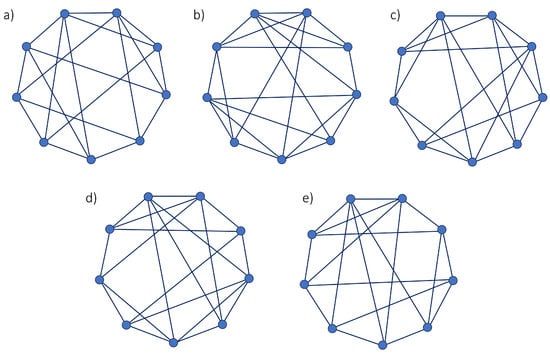  Figure 4. (a–e) Illustration of the five GLGs with nine vertices.

In Table 2, we indicate some of the properties of these GLGs with nine vertices, following the same notation as in Table 1.

Table 2. Properties of the GLGs with $n=9$ vertices.

#	m	$\mathit{\delta }$	$\Delta$	D	ind	${\mathit{\kappa }}_{\mathit{v}}$	${\mathit{\kappa }}_{\mathit{e}}$	$\mathit{\omega }$	$\mathit{\gamma }$	H	P	M	r	p
a	19	4	5	2	3	4	4	3	2	Y	Y	Y	N	N
b	21	4	5	2	3	4	4	4	2	Y	Y	Y	N	N
c	20	4	5	2	3	4	4	3	2	Y	Y	Y	N	N
d	20	4	5	2	3	4	4	4	2	Y	Y	Y	N	N
e	19	4	5	2	3	4	4	3	2	Y	Y	Y	N	N

• There are 102 GLGs among the 11,716,571 connected graphs with $n=10$ vertices. (The adjacency matrices (in MATLAB format) and a table with the properties of GLGs with ten vertices can be requested to the main author via email).

We now resume our computational observations for the GLGs described in Table 1 and Table 2.

• The fifteen GLG with eight vertices, five GLGs with nine vertices, and 102 GLGs with ten vertices have the following general properties:
  • For all of these graphs, ${\mu }_n=5+\sqrt{5}$ and ${\mu }_2=5-\sqrt{5}$.
  • They are all Hamiltonian; notice that all GLGs with $n\le 10$ are pancyclic except for the one with adjacency matrix $A\left(C_5\right)\otimes J_2$, where ⊗ is the Kronecker product and $J_2$ is the all-ones matrix of order 2 (see the next section for details of this operation).
  • They have a perfect (even n) or nearly-perfect matching (odd n), as evident from the fact that all of these GLGs have a Hamiltonian cycle, which implies the existence of a perfect matching.
  • They have diameter 2.
  • They have clique number $3\le \omega \le 4$.
  • They have ${\kappa }_v={\kappa }_e=\delta$, except for the graph with adjacency matrix $\left(A\left(C_5\right)+I_5\right)\otimes J_2-I_{10}$ (see the next section for details of this operation).
  • They have minimum degree $\delta \ge 3$.
  • They have domination number 2 ($n\le 9$) or $2\le \gamma \le 3$ ($n=10$); notice that if $\delta \ge 3$, then (according to Reed [32]) $\gamma \ge {\displaystyle \frac{3n}{8}}$, which is the bound observed for $n\le 10$.
  • They have independence number $2\le ind\le 4$; notice that $ind\ge {\displaystyle \frac{n}{\overline{l}+1}}$ [33,34], where $\overline{l}$ is the average shortest path distance in G. Thus, if $2=D\ge \overline{l}$, as observed for these GLGs, $ind\ge {\displaystyle \frac{n}{3}}$.

5. Expanding the Family of GLGs

Having some GLGs such as those found in the previous section, we are now interested in constructing new ones on the same basis. For this, we mainly use the Kronecker product of the adjacency matrix of a GLG along with the all-ones matrix. Let $J_r$ and $I_r$ be the all-ones and identity matrices of order r, respectively. We state here the following known facts which are used in the forthcoming results. The first is proved on p. 442 of [17].

Lemma 18.

Let X and Y be two matrices with spectra $spec\left(X\right)=\left\{{\lambda }_i\left(X\right),i=1,\cdots ,r\right\}$ and $spec\left(Y\right)=\left\{{\lambda }_j\left(Y\right),j=1,\cdots ,s\right\}$, where ${\lambda }_i\left(X\right)$ and ${\lambda }_j\left(Y\right)$ are the eigenvalues of X and Y, respectively. Then, the spectrum of the Kronecker product of the two matrices is $spec\left(X\otimes Y\right)=\left\{{\lambda }_i\left(X\right){\lambda }_j\left(Y\right),ij=1,\cdots ,rs\right\}$.

The following result is proved in [35].

Lemma 19.

Let X and Y be two Hermitian matrices of the same order r such that $XY=YX$; then, there exist permutations a and b of $\left\{1,\dots ,r\right\}$ ${\lambda }_k\left(X+Y\right)=\left\{{\lambda }_{a\left(k\right)}\left(X\right)+{\lambda }_{b\left(k\right)}\left(Y\right)\right\}$ for all $k=1,\cdots ,r$.

We now define some classes of graphs using the Kronecker product of their adjacency matrices and some standard matrices.

Definition 2.

Let G be a graph with adjacency and Laplacian matrices A and L, respectively. Let $\tilde{G}$ be a graph with an adjacency matrix $\tilde{A}$ constructed as follows:

$$\tilde{A}A\otimes J_r,$$

(52)

where ⊗ is the Kronecker product.

We now have the following result.

Theorem 2.

The spectrum of the Laplacian matrix $\tilde{L}$ of $\tilde{G}$ is provided by

$$\mathrm{spec}\left(\tilde{L}\right)=\mathrm{spec}\left(L\otimes J_r\right)-\mathrm{spec}\left(K\otimes \left(J_r-r{I}_r\right)\right).$$

(53)

Proof. 

First, we can write $\tilde{L}=\tilde{K}-\tilde{A}$, where $\tilde{K}=rK\otimes I_r$. Then, we have

$$\begin{array}{cc}\hfill \tilde{L}& =rK\otimes I_r-A\otimes J_r\hfill \\ \hfill & =rK\otimes I_r-A\otimes J_r+K\otimes J_r-K\otimes J_r\hfill \\ \hfill & =\left(K-A\right)\otimes J_r+K\otimes \left(r{I}_r-J_r\right)\hfill \\ \hfill & =\left(K-A\right)\otimes J_r-K\otimes \left(J_r-r{I}_r\right).\hfill \end{array}$$

(54)

Now, designating $PL\otimes J_r$ and $QK\otimes \left(r{I}_r-J_r\right)$, we can see that

$$\begin{array}{cc}\hfill PQ& =\left(L\otimes J_r\right)\left(K\otimes \left(r{I}_r-J_r\right)\right)\hfill \\ \hfill & =LK\otimes \left(J_r\left(r{I}_r-J_r\right)\right)\hfill \\ \hfill & =LK\otimes r{J}_r-LK\otimes J_r^2\hfill \end{array}$$

(55)

and

$$\begin{array}{cc}\hfill QP& =\left(K\otimes r{I}_r-J_r\right)\left(L\otimes J_r\right)\hfill \\ \hfill & =KL\otimes \left(\left(r{I}_r-J_r\right)J_r\right)\hfill \\ \hfill & =KL\otimes r{J}_r-KL\otimes J_r^2.\hfill \end{array}$$

(56)

Notice that, because $J_r^2=r{J}_r$, $PQ=QP=0$; consequently, because P and Q commute, we have $\mathrm{spec}\left(\tilde{L}\right)=\mathrm{spec}\left(P-Q\right)=\mathrm{spec}\left(P\right)-\mathrm{spec}\left(Q\right)$, which proves the result. □

Theorem 3.

Let G be a GLG with adjacency matrix A; then the graph $\tilde{G}$ with the adjacency matrix obtained as $\tilde{A}A\otimes J_r$ is a GLG.

Proof. 

We start from the fact that $\mathrm{spec}\left(\tilde{L}\right)=\mathrm{spec}\left(P\right)-\mathrm{spec}\left(Q\right)$. First, we consider

$$\mathrm{spec}\left(P\right)=\mathrm{spec}\left(L\otimes J_r\right)=\left\{{\mu }_i\left(L\right){\lambda }_j\left(J_r\right),ij=1,\dots ,rn\right\}.$$

(57)

Similarly,

$$\mathrm{spec}\left(Q\right)=\mathrm{spec}\left(K\otimes r{I}_r-J_r\right)=\left\{{\lambda }_i\left(K\right){\lambda }_j\left(r{I}_r-J_r\right),ij=1,\dots ,rn\right\}.$$

(58)

Because the eigenvalues $0={\tilde{\mu }}_1<{\tilde{\mu }}_2\le \cdots \le {\tilde{\mu }}_{rn}$ of $\tilde{L}$ are the difference of those of P and Q, we have

$$\mathrm{spec}\left(\tilde{L}\right)=\left\{{\tilde{\mu }}_n=max\left\{{\lambda }_n\left(P\right),{\lambda }_n\left(Q\right)\right\},\dots ,{\tilde{\mu }}_2=min\left\{{\lambda }_1\left(P\right),{\lambda }_1\left(Q\right)\right\},0\right\}.$$

(59)

The largest eigenvalue of P is ${\lambda }_{nr}\left(P\right)=r{\mu }_n\left(L\right)$, while that of Q is ${\lambda }_{nr}\left(Q\right)=\Delta r$. Thus, because ${\mu }_n\left(L\right)\ge \Delta +1$, we have

$${\tilde{\mu }}_{nr}=max\left\{{\lambda }_n\left(P\right),{\lambda }_n\left(Q\right)\right\}=r{\mu }_n\left(L\right).$$

(60)

Similarly, we have ${\lambda }_1\left(P\right)=r{\mu }_2\left(L\right)$ and ${\lambda }_1\left(Q\right)=\delta r$; therefore, because ${\mu }_2\left(L\right)\le \delta$, we have

$${\tilde{\mu }}_2=min\left\{{\lambda }_1\left(P\right),{\lambda }_1\left(Q\right)\right\}=r{\mu }_2\left(L\right).$$

(61)

Therefore,

$${\displaystyle \frac{{\tilde{\mu }}_{nr}}{{\tilde{\mu }}_2}}={\displaystyle \frac{{\mu }_n\left(L\right)}{{\mu }_2\left(L\right),}}$$

(62)

and if ${\mu }_n\left(L\right)/{\mu }_2\left(L\right)=\phi +1$, it is the same for ${\tilde{\mu }}_{nr}\left(L\right)/{\tilde{\mu }}_2\left(L\right).$ □

Proposition 1.

Let G be a graph with adjacency and Laplacian matrices A and L, respectively. Let $J_r$ and $I_r$ be the all-ones and identity matrices of order r, respectively, and let $\widehat{G}$ be the graph with adjacency matrix $\widehat{A}$ constructed as follows:

,

(63)

where ⊗ is the Kronecker product and the eigenvalues of L are denoted by $0={\mu }_1<{\mu }_2\le \cdots \le {\mu }_n$.

We then have the following result.

Theorem 4.

Let G be a GLG with adjacency matrix A; then, the graph $\widehat{G}$ with adjacency matrix obtained as $\widehat{A}A$ J_r is a GLG.

Proof. 

The Laplacian matrix of $\widehat{G}$ is

$$\widehat{L}=rK\otimes I_r-\left(A+I_n\right)\otimes J_r+r\left(I_n\otimes I_r\right),$$

(64)

where $I_n$ is the identity matrix of the same dimension as A. Then, by summing and subtracting $K\otimes J_r$, we have

$$\begin{array}{cc}\hfill \widehat{L}& =r\left(K+I_n\right)\otimes I_r+K\otimes J_r-A\otimes J_r-K\otimes J_r-I_n\otimes J_r\hfill \\ \hfill & =\left(K+I_n\right)\otimes I_r+L\otimes J_r-\left(K+I_n\right)\otimes J_r\hfill \\ \hfill & =L\otimes J_r-\left(K+I_n\right)\otimes \left(J_r-r{I}_r\right).\hfill \end{array}$$

(65)

Letting $P=L\otimes J_r$ and $R=\left(K+I_n\right)\otimes \left(J_r-r{I}_r\right)$, we have

$$\begin{array}{cc}\hfill PR& =\left(L\otimes J_r\right)\left(\left(K+I_n\right)\otimes \left(J_r-r{I}_r\right)\right)\hfill \\ \hfill & =L\left(K+I_n\right)\otimes \left(J_r\left(J_r-r{I}_r\right)\right)\hfill \\ \hfill & =L\left(K+I_n\right)\otimes \left(r{J}_r-r{J}_r\right)\hfill \\ \hfill & =0_n\hfill \end{array}$$

(66)

and

$$\begin{array}{cc}\hfill RP& =\left(\left(K+I_n\right)\otimes \left(J_r-r{I}_r\right)\right)\left(L\otimes J_r\right)\hfill \\ \hfill & =\left(K+I_n\right)L\otimes \left(J_r-r{I}_r\right)J_r\hfill \\ \hfill & =\left(K+I_n\right)L\otimes \left(r{J}_r-r{J}_r\right)\hfill \\ \hfill & =0_n,\hfill \end{array}$$

(67)

where $0_n$ is the zero matrix of order n. Therefore, $PR=RP=0$, and we have $\mathrm{spec}\left(\widehat{L}\right)=\mathrm{spec}\left(P-R\right)=\mathrm{spec}\left(P\right)-\mathrm{spec}\left(R\right)$.

Similarly,

$$\mathrm{spec}\left(R\right)=\mathrm{spec}\left(\left(K+I_n\right)\otimes \left(J_r-r{I}_r\right)\right)=\left\{{\lambda }_i\left(K+I_n\right){\lambda }_j\left(J_r-r{I}_r\right),ij=1,\dots ,rn\right\}.$$

(68)

Because the eigenvalues $0={\widehat{\mu }}_1<{\widehat{\mu }}_2\le \cdots \le {\widehat{\mu }}_{rn}$ of $\widehat{L}$ are the difference of those of P and R, we have

$$\mathrm{spec}\left(\widehat{L}\right)=\left\{{\widehat{\mu }}_{rn}=max\left\{{\lambda }_n\left(P\right),{\lambda }_n\left(R\right)\right\},\dots ,{\widehat{\mu }}_2=min\left\{{\lambda }_1\left(P\right),{\lambda }_1\left(R\right)\right\},0\right\}.$$

(69)

The largest eigenvalue of P is ${\lambda }_{nr}\left(P\right)=r{\mu }_n\left(L\right)$, while that of R is ${\lambda }_{nr}\left(R\right)=\left(\Delta +1\right)r$. Thus, because ${\mu }_n\left(L\right)\ge \Delta +1$, we have

$${\widehat{\mu }}_{rn}=max\left\{{\lambda }_n\left(P\right),{\lambda }_n\left(R\right)\right\}=r{\mu }_n\left(L\right).$$

(70)

Similarly, we have ${\lambda }_1\left(P\right)=r{\mu }_2\left(L\right)$ and ${\lambda }_1\left(R\right)=\left(\delta +1\right)r$; therefore, because ${\mu }_2\left(L\right)\le \delta$, we have

$${\widehat{\mu }}_2=min\left\{{\lambda }_1\left(R\right),{\lambda }_1\left(S\right)\right\}=r{\mu }_2\left(L\right).$$

(71)

Therefore,

$${\displaystyle \frac{{\widehat{\mu }}_{rn}}{{\widehat{\mu }}_2}}={\displaystyle \frac{{\mu }_n\left(L\right)}{{\mu }_2\left(L\right)}},$$

(72)

which proves the result. □

6. Synchronization of GLGs

GLGs have interesting synchronization properties. To illustrate them, we can consider a set of dynamical oscillators coupled by a GLG. Each oscillator i (with $i=1,\dots ,n$) is characterized by a state vector ${\mathbf{x}}_i\left(t\right)\in {\mathbb{R}}^s$, where s is the size of the state vector. The dynamics of the state vector are described by the following equation:

$${\dot{\mathbf{x}}}_i=\mathbf{f}\left({\mathbf{x}}_i\right)-\sigma {\displaystyle \sum _{j=1}^n}{L}_{ij}\mathbf{h}\left({\mathbf{x}}_j\right),$$

(73)

where $\mathbf{f}:{\mathbb{R}}^s\to {\mathbb{R}}^s$ represents the uncoupled dynamics of the dynamical oscillator, $\mathbf{h}:{\mathbb{R}}^s\to {\mathbb{R}}^s$ is the coupling function, and $\sigma$ is the coupling strength.

We say that the system in (73) is synchronized if all of the oscillators asymptotically converge to the same trajectory, that is, $\underset{t\to +\infty }{lim}\parallel {\mathbf{x}}_i\left(t\right)-{\mathbf{x}}_j\left(t\right)\parallel =0$ for any pair of oscillators i and j. In a generic system of coupled oscillators, a linear analysis of the stability of synchronization carried out with the master stability function approach shows that there are two types of systems that can synchronize [19,20]. The first, called class II systems, has an unbounded synchronized region specified by $\sigma {\mu }_2>{\nu }_1>0$, where the constant ${\nu }_1$ only depends on the node dynamics and coupling function, namely, $\mathbf{f}$ and $\mathbf{h}$. The second, called class III systems, has a bounded synchronized region specified by $\sigma {\mu }_2,\dots ,\sigma {\mu }_n\in ({\nu }_1,{\nu }_2)\subset (0,\infty )$, where the constants ${\nu }_1$ and ${\nu }_2$ only depend on the node dynamics and coupling function. Notice that class II systems can always be synchronized provided that the coupling strength is large enough. On the contrary, class III system can only be synchronized if ${\mu }_n/{\mu }_2<{\nu }_2/{\nu }_1$. The ratio $\mathcal{Q}={\mu }_n/{\mu }_2$ is known in the field as the graph eigenratio.

Remark 2.

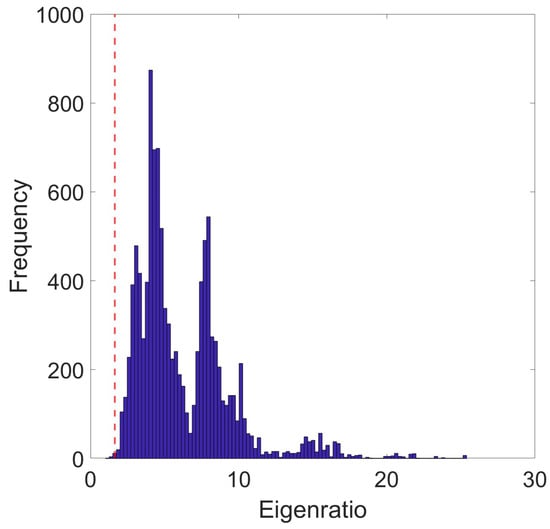
For graphs with $n=8$, the mean eigenratio is $\overline{Q}\approx 6.24\pm 3.26$. However, the graphs for which $\mathcal{Q}={\phi }^2$ are among the top 3.32% of eight-vertex graphs with the smallest $\mathcal{Q}$, and consequently are in the corresponding top percentage of most synchronizable graphs (see Figure 5); this percentage is $2.52\%$ for $n=9$ and $1.64\%$ for $n=10.$

Figure 5. Histogram of the values of the eigenratio $\mathcal{Q}$ of the 11,117 connected graphs with eight vertices. The graphs with Q equal to the square of the golden ratio are marked as a vertical broken line. Only those graphs having $\mathcal{Q}$ below this line are more synchronizable than GLGs.

We now discuss some results on synchronization in GLGs. If we know that a graph is a GLG, then we know its region of synchronization. In fact, for class II systems we have the following proposition.

Proposition 2.

Consider a class II system of dynamical oscillators, such as the one in (73), coupled by a GLG. Then, a necessary condition for synchronization in the graph is that

$$\sigma >\frac{{\nu }_1}{{\mu }_2}=\frac{{\phi }^2{\nu }_1}{{\mu }_n},$$

(74)

which, when ${\mu }_2=k\frac{5-\sqrt{5}}{2}$ and $k=1,2\dots$, is provided by

$$\sigma >\frac{2{\nu }_1}{k(5-\sqrt{5})}.$$

(75)

Proof. 

The proof directly follow from the property that ${\mu }_2=k\frac{5-\sqrt{5}}{2}$ for any GLG. □

For class III systems, we have the following result.

Proposition 3.

Consider a class III system of dynamical oscillators such as the one in (73) coupled by a GLG. Then, a necessary condition for synchronization in the graph is that

$${\phi }^2<\frac{{\nu }_2}{{\nu }_1}$$

(76)

and

$$\frac{{\nu }_1}{{\mu }_2}<\sigma <\frac{{\nu }_2}{{\phi }^2{\mu }_2}$$

(77)

or that

$$\frac{{\phi }^2{\nu }_1}{{\mu }_n}<\sigma <\frac{{\nu }_2}{{\mu }_n}.$$

(78)

If ${\mu }_2=k\frac{5-\sqrt{5}}{2}$, $k=1,2\dots$, then

$$\frac{2{\nu }_1}{k(5-\sqrt{5})}<\sigma <\frac{2{\nu }_2}{k(5+\sqrt{5})}.$$

(79)

Proof. 

The proof directly follow from the property that $\frac{{\mu }_n}{{\mu }_2}={\phi }^2$ and ${\mu }_2=k\frac{5-\sqrt{5}}{2}$ for any GLG. □

As discussed above, not all class III systems are synchronizable. Here, we illustrate a fascinating result showing how many well-known chaotic circuits are in fact synchronizable when coupled by any GLG. A few examples are listed in Table 3. Quite remarkably, the table includes many relevant examples of paradigmatic chaotic circuits, such as the Lorenz system [36], the Rossler equation [37], the Chua’s circuit [38], and the Chen system [39].

Table 3. List of a series of class III systems, along with their equations, coupling type, and parameters ${\nu }_1$, ${\nu }_2$, and ${\nu }_2/{\nu }_1$ for which ${\nu }_2/{\nu }_1<{\phi }^2$. All of these graphs are synchronizable when coupled by any GLG. For the Chua’s circuit, $f\left(x\right)=\left\{\begin{array}{cc}-bx-a+b,\hfill & x>1\\ -ax,\hfill & \left|x\right|<1\\ -bx-a+b,\hfill & x<-1\end{array}\right.$ with $a=-1.27$ and $b=-0.68$. The notation $i\to j$ indicates that the i-th variable of one oscillator is coupled to the dynamics of the j-th variable of the other oscillator (linear diffusive coupling is always assumed here). Data on the values of ${\nu }_1$ and ${\nu }_2$ are taken from [40].

System	Equations	Coupling	${\mathit{\nu }}_1$	${\mathit{\nu }}_2$	${\mathit{\nu }}_2/{\mathit{\nu }}_1$
Rossler	$$\begin{array}{c}\dot{x}=-y-z\hfill \\ \dot{y}=x+0.2y\hfill \\ \dot{z}=0.2+(x-9)z\hfill \end{array}$$	$1\to 1$	0.186	4.614	24.807
Lorenz	$$\begin{array}{c}\dot{x}=10(y-x)\hfill \\ \dot{y}=x(28-z)-y\hfill \\ \dot{z}=xy-\frac{8}{3}z\hfill \end{array}$$	$2\to 1$	3.98	23.692	5.953
Chen	$$\begin{array}{c}\dot{x}=35(y-x)\hfill \\ \dot{y}=(-7-z)x+cy\hfill \\ \dot{z}=xy-\frac{8}{3}z\hfill \end{array}$$	$3\to 3$	5.347	21.51	4.023
Chua	$$\begin{array}{c}\dot{x}=10[y-x+f\left(x\right)]\hfill \\ \dot{y}=x-y+z\hfill \\ \dot{z}=-14.87y\hfill \end{array}$$	$3\to 3$	0.788	4.82	6.117
Hindmarsh-Rose	$$\begin{array}{c}\dot{x}=y+3x^2-x^3-z+3.2\hfill \\ \dot{y}=1-5x^2-y\hfill \\ \dot{z}=0.006[-z+4(x+1.6)]\hfill \end{array}$$	$2\to 1$	0.286	1.233	4.311

Finally, we discuss a numerical example illustrating synchronization in a system of $n=10$ Rossler oscillators coupled by a GLG. The system is described by the following equations:

$$\begin{array}{c}{\dot{x}}_i=-y_i-z_i-\sigma {\displaystyle \sum _{j=1}^n}{L}_{ij}{x}_j\hfill \\ {\dot{y}}_i=x_i+0.2y_i\hfill \\ {\dot{z}}_i=0.2+(x_i-9)z_i\hfill \end{array}$$

(80)

with $i=1,\dots ,n$.

We consider two GLGs, for each of which we calculate the synchronization error $E={⟨\frac{1}{n-1}{\displaystyle \sum _{j=2}^n}\frac{|x_j-x_1|+|y_j-y_2|+|z_j-z_1|}{3}⟩}_T$ for different values of $\sigma$ (here, T represents a sufficiently large window of time after the transient dynamics have vanished). Figure 6 illustrates the results, showing that the two GLGs have the same synchronization region.

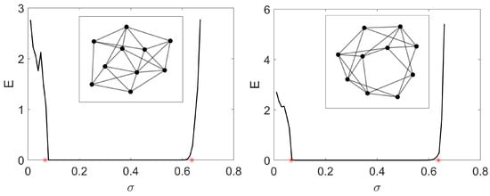
Figure 6. Synchronization error E vs. coupling coefficient $\sigma$ for two networks of $n=10$ coupled Rossler oscillators, as in (80). Both GLGs (shown in the insets of panels (left) and (right)) display the same region of stability for synchronization, as $k=2$ for both of them. Red asterisks mark the predicted thresholds for synchronization based on the master stability function approach, as in Equation (79) with $k=2$.

7. Conclusions and Future Outlook

By representing the eigenvalues of the Laplacian matrix of a graph as a line segment, we have asked a general mathematical question about the ratios between the length of the spectrum ${\mu }_n-{\mu }_1$ and its spread ${\mu }_n-{\mu }_2$ as well as between the latter and ${\mu }_2-{\mu }_1$. We have discovered here that graphs exist for which these two ratios are identical, and consequently equal to the golden ratio. We have found all of the graphs having this property, for which we have proposed the name of Golden Laplacian Graphs (GLG), with at most ten vertices. We have analytically proved upper and lower bounds for several algebraic and graph-theoretic properties of GLG, enumerated several properties of the discovered GLGs, and proved the existence of methods to expand GLGs to larger sizes. However, there are many open and intriguing questions emerging from this work. We enumerate several of these below to encourage the reader to investigate them further.

Which structural characteristic(s) differentiate GLGs from other graphs?

Do all GLG have a diameter equal to 2?

Are all GLGs Hamiltonian? What are the condition(s) for them to be pancyclic? If they are not Hamiltonian, do they still have a perfect matching (even n) or a nearly-perfect matching (odd n)?

Are there GLGs with a clique number larger than 4? Which condition should the clique number obey in GLGs?

References

- Biggs, N. Algebraic Graph Theory; Number 67; Cambridge University Press: Cambridge, UK, 1993. [Google Scholar]
- Godsil, C.; Royle, G.F. Algebraic Graph Theory; Springer Science & Business Media: Berlin/Heidelberg, Germany, 2001; Volume 207. [Google Scholar]
- Van Mieghem, P. Graph Spectra for Complex Networks; Cambridge University Press: Cambridge, UK, 2023. [Google Scholar]
- Jamakovic, A.; Van Mieghem, P. On the robustness of complex networks by using the algebraic connectivity. In Proceedings of the NETWORKING 2008 Ad Hoc and Sensor Networks, Wireless Networks, Next Generation Internet: 7th International IFIP-TC6 Networking Conference, Singapore, 5–9 May 2008; Proceedings 7. Springer: Berlin/Heidelberg, Germany, 2008; pp. 183–194. [Google Scholar]
- Mohar, B. Isoperimetric numbers of graphs. J. Comb. Theory Ser. 1989, 47, 274–291. [Google Scholar] [CrossRef]
- Masuda, N.; Porter, M.A.; Lambiotte, R. Random walks and diffusion on networks. Phys. Rep. 2017, 716, 1–58. [Google Scholar] [CrossRef]
- Arenas, A.; Díaz-Guilera, A.; Kurths, J.; Moreno, Y.; Zhou, C. Synchronization in complex networks. Phys. Rep. 2008, 469, 93–153. [Google Scholar] [CrossRef]
- Xiao, W.; Gutman, I. Resistance distance and Laplacian spectrum. Theor. Chem. Accounts 2003, 110, 284–289. [Google Scholar] [CrossRef]
- Boyd, S. Convex optimization of graph Laplacian eigenvalues. In Proceedings of the International Congress of Mathematicians, Madrid, Spain, 22–30 August 2006; Volume 3, pp. 1311–1319. [Google Scholar]
- Donetti, L.; Hurtado, P.I.; Munoz, M.A. Entangled networks, synchronization, and optimal network topology. Phys. Rev. Lett. 2005, 95, 188701. [Google Scholar] [CrossRef]
- Donetti, L.; Neri, F.; Munoz, M.A. Optimal network topologies: Expanders, cages, Ramanujan graphs, entangled networks and all that. J. Stat. Mech. Theory Exp. 2006, 2006, P08007. [Google Scholar] [CrossRef]
- Marples, C.R.; Williams, P.M. The Golden Ratio in Nature: A Tour Across Length Scales. Symmetry 2022, 14, 2059. [Google Scholar] [CrossRef]
- Estrada, E. Graphs (networks) with golden spectral ratio. Chaos Solitons Fractals 2007, 33, 1168–1182. [Google Scholar] [CrossRef]
- Estrada, E.; Gago, S.; Caporossi, G. Design of highly synchronizable and robust networks. Automatica 2010, 46, 1835–1842. [Google Scholar] [CrossRef]
- Watts, D.J.; Strogatz, S.H. Collective dynamics of ‘small-world’networks. Nature 1998, 393, 440–442. [Google Scholar] [CrossRef]
- Gross, J.L.; Yellen, J. Handbook of Graph Theory; CRC Press: Boca Raton, FL, USA, 2003. [Google Scholar]
- Bernstein, D.S. Matrix Mathematics: Theory, Facts, and Formulas; Princeton University Press: Princeton, NJ, USA, 2009. [Google Scholar]
- Horn, R.A.; Johnson, C.R. Matrix Analysis; Cambridge University Press: Cambridge, UK, 2012. [Google Scholar]
- Boccaletti, S.; Latora, V.; Moreno, Y.; Chavez, M.; Hwang, D.U. Complex networks: Structure and dynamics. Phys. Rep. 2006, 424, 175–308. [Google Scholar] [CrossRef]
- Pecora, L.M.; Carroll, T.L. Master stability functions for synchronized coupled systems. Phys. Rev. Lett. 1998, 80, 2109. [Google Scholar] [CrossRef]
- Stanić, Z. Inequalities for Graph Eigenvalues; Cambridge University Press: Cambridge, UK, 2015; Volume 423. [Google Scholar]
- Grone, R.; Merris, R. Algebraic connectivity of trees. Czechoslov. Math. J. 1987, 37, 660–670. [Google Scholar] [CrossRef]
- Mohar, B.; Alavi, Y.; Chartrand, G.; Oellermann, O. The Laplacian spectrum of graphs. Graph Theory Comb. Appl. 1991, 2, 12. [Google Scholar]
- Zhu, D. On upper bounds for Laplacian graph eigenvalues. Linear Algebra Its Appl. 2010, 432, 2764–2772. [Google Scholar] [CrossRef][Green Version]
- Fiedler, M. Algebraic connectivity of graphs. Czechoslov. Math. J. 1973, 23, 298–305. [Google Scholar] [CrossRef]
- Brouwer, A.E.; Haemers, W.H. Spectra of Graphs; Springer Science & Business Media: Berlin/Heidelberg, Germany, 2011. [Google Scholar]
- Mohar, B. Eigenvalues, diameter, and mean distance in graphs. Graphs Comb. 1991, 7, 53–64. [Google Scholar] [CrossRef]
- Chung, F.R.; Faber, V.; Manteuffel, T.A. An upper bound on the diameter of a graph from eigenvalues associated with its Laplacian. SIAM J. Discret. Math. 1994, 7, 443–457. [Google Scholar] [CrossRef]
- Lu, M.; Liu, H.; Tian, F. Laplacian spectral bounds for clique and independence numbers of graphs. J. Comb. Theory Ser. 2007, 97, 726–732. [Google Scholar] [CrossRef]
- Gu, X.; Liu, M. A tight lower bound on the matching number of graphs via Laplacian eigenvalues. Eur. J. Comb. 2022, 101, 103468. [Google Scholar] [CrossRef]
- Vajda, S. Fibonacci and Lucas Numbers, and the Golden Section: Theory and Applications; Courier Corporation: Chelmsford, MA, USA, 2008. [Google Scholar]
- Reed, B. Paths, stars and the number three. Comb. Probab. Comput. 1996, 5, 277–295. [Google Scholar] [CrossRef]
- Turán, P. On the theory of graphs. Colloq. Math. 1954, 1, 19–30. [Google Scholar] [CrossRef]
- Griggs, J.R.; Kleitman, D.J. Independence and the Havel-Hakimi residue. Discret. Math. 1994, 127, 209–212. [Google Scholar] [CrossRef]
- So, W. Commutativity and spectra of Hermitian matrices. Linear Algebra Its Appl. 1994, 212, 121–129. [Google Scholar] [CrossRef]
- Lorenz, E.N. Deterministic nonperiodic flow. J. Atmos. Sci. 1963, 20, 130–141. [Google Scholar] [CrossRef]
- Rössler, O.E. An equation for continuous chaos. Phys. Lett. A 1976, 57, 397–398. [Google Scholar] [CrossRef]
- Matsumoto, T.; Chua, L.; Komuro, M. The double scroll. IEEE Trans. Circuits Syst. 1985, 32, 797–818. [Google Scholar] [CrossRef]
- Chen, G.; Ueta, T. Yet another chaotic attractor. Int. J. Bifurc. Chaos 1999, 9, 1465–1466. [Google Scholar] [CrossRef]
- Huang, L.; Chen, Q.; Lai, Y.C.; Pecora, L.M. Generic behavior of master-stability functions in coupled nonlinear dynamical systems. Phys. Rev. E 2009, 80, 036204. [Google Scholar] [CrossRef]
Disclaimer/Publisher’s Note: The statements, opinions and data contained in all publications are solely those of the individual author(s) and contributor(s) and not of MDPI and/or the editor(s). MDPI and/or the editor(s) disclaim responsibility for any injury to people or property resulting from any ideas, methods, instructions or products referred to in the content. |
© 2024 by the authors. Licensee MDPI, Basel, Switzerland. This article is an open access article distributed under the terms and conditions of the Creative Commons Attribution (CC BY) license (https://creativecommons.org/licenses/by/4.0/).