Study on Exchange Rate Forecasting with Stacked Optimization Based on a Learning Algorithm

Abstract

The time series of exchange rate fluctuations are characterized by non-stationary and nonlinear features, and forecasting using traditional linear or single-machine models can cause significant bias. Based on this, the authors propose the combination of the advantages of the EMD and LSTM models to reduce the complexity by analyzing and decomposing the time series and forming a new model, EMD-LSTM-SVR, with a stronger generalization ability. More than 30,000 units of data on the USD/CNY exchange rate opening price from 2 January 2015 to 30 April 2022 were selected for an empirical demonstration of the model’s accuracy. The empirical results showed that the prediction of the exchange rate fluctuation with the EMD-LSTM-SVR model not only had higher accuracy, but also ensured that most of the predicted positions deviated less from the actual positions. The new model had a stronger generalization ability, a concise structure, and a high degree of ability to fit nonlinear features, and it prevented gradient vanishing and overfitting to achieve a higher degree of prediction accuracy.

1. Introduction

Researchers and scholars have applied various statistical methods and econometric models to the prediction of exchange rate fluctuations. The most-popular methods in current research mainly include the single-integer auto-regressive moving average (ARIMA) model [1], the auto-regressive conditional heteroskedasticity (ARCH) model [2], the generalized auto-regressive conditional heteroskedasticity (GARCH) model [3], and the threshold auto-regressive (TAR) model [4], among others. These methods mostly utilize a single model to complete predictions while paying more attention to local information. It is easy for them to fit a standard time series when dealing with smoother and fewer data, thus allowing them to reach a prediction. However, for complex nonlinear exchange rates, these models cannot achieve accurate predictions. Existing research shows that foreign exchange market returns do not obey a normal distribution, as they typically have sharp peaks and thick tails. In foreign exchange time series, the fluctuations are very significantly non-stationary, nonlinear, and history-dependent [5]. Therefore, when forecasting foreign exchange, the assumptions of traditional linear models cannot be satisfied. So, the application of forecasting with a traditional model may cause significant deviations [6]. Based on this, machine learning models began to be gradually used in exchange rate forecasting. In the existing literature, most studies proposed either the combination of linear models and machine learning models [7] or combinations of several machine learning algorithms for stacked optimization [8]. The research was biased towards improving the models from the technical point of view, but few studies were conducted to improve the models in terms of the characteristics of the financial market. Deep learning models have many advantages over machine learning for the forecasting of nonlinear time series [9]. Without any assumptions about the time structure, they can find highly nonlinear and complex dependencies in a time series and have the advantage of processing and memorizing nonlinear feature data themselves, which has caused them to quickly attract much attention. Wenhui Dai (2017) built a VAR estimation model by combining deep learning LSTM, DBN, and ARMA-GARCH models, and they used seven common types of exchange rate data to confirm that the model was accurate and reliable [10]. Huang Jiahui (2022) optimized their model by constructing a composite network that decomposed raw serial data on the exchange rate before training it using an LSTM-based model, and the results showed the model’s better prediction capabilities and optimization [11]. Zhang Lei (2021) added the VIX index, which represented sentiment, to an LSTM neural network for exchange rate prediction, and the results showed that the model was able to improve the prediction accuracy to a certain extent compared with the traditional volatility prediction method [12]. Another way to improve a prediction model consists of using an attention mechanism. This mechanism can automatically obtain the input time point that best determines the forecast value at the current moment. This can optimize the neural network structure to better take the temporal dependence into account, thus allowing further improvement of the prediction accuracy in long-term forecasting [13]. The aforementioned research results laid the foundation for this work. However, research gaps exist when attempting to answer the following question: How can one effectively decompose the exchange rate in these kinds of non-smooth, nonlinear serial-data time series containing some noise to improve the accuracy of forecasting?

In order to address the drawbacks of the use of a single model, a new EMD-LSTM-SVR model is proposed. It was formed to draw on the advantages of EMD and LSTM models. The empirical modal decomposition (EMD) method not only has the advantages of good resolution, directness, adaptability, and a posteriori function, but its basis function can also be derived from its own decomposition of the data. So, there is no need to pre-compute and pre-specify the basis function [14]. The LSTM, an improved recurrent neural network, can learn long-term memory information and optimize a problem through gradient disappearance [15]. The proposed model should portray a stronger generalization ability, simpler structure, greater ability to fit nonlinear features, and better prevention of gradient vanishing and overfitting, which should improve the learning ability to achieve a higher degree of prediction accuracy.

In order to verify and confirm the efficiency of the proposed model, we selected more than 30,000 units of data on the USD/CNY exchange rate opening price from 2 January 2015 to 30 April 2022, for model measurement. We show through experiments that the use of a deep-learning-based LSTM model in the exchange rate series prediction was able to effectively improve the prediction accuracy. The prediction results showed that, relative to the BP and LSTM models, the average absolute percentage errors of the prediction results of the EMD-LSTM-SVR model were reduced by 21.03% and 14.72%, respectively, thus improving the effect by 43.93% and 33.08%, respectively. Moreover, the standard deviation was closer to the average error than that of the BP and LSTM models. So, the proposed EMD-LSTM-SVR model for the prediction of exchange rate fluctuations not only had higher prediction accuracy, but also ensured that most of the predicted positions deviated less from the actual ones.

The research results in this work relate to the traditional methods of forecasting nonlinear exchange rate fluctuations, which is a more-complex prediction task, and a sequence prediction method using deep learning was optimized, as this can increase the complexity of a neural network model for the achievement of the function of accurate prediction. In addition, sequence prediction based on deep learning is an existential supervised learning technique that does not require the creation of time series features through human labeling, so it saves much of the workload in comparison with traditional methods. It goes without saying that the research results in this work are also of great significance for the effective prevention of economic risks due to exchange rate fluctuations.

The rest of this paper is organized into six sections: First, in Section 2, we introduce the related technologies involved in this work and establish the foundation for the next step of building the framework of the proposed model. Then, in Section 3, we present the idea behind establishing a new model according to the characteristics of exchange rate fluctuations through the construction of related technology. The model parameters are optimized, and the exchange rate prediction model is established. After that, in Section 4, we describe the dataset used in the experiments and present the accuracy of the model as empirical evidence. Later, in Section 5, we select and present the evaluation indexes and analyze, discuss, and compare the obtained results. Finally, in Section 6, we summarize the findings of this work and discuss the possible further improvement of the model.

2. Related Technologies

In this section, we review some of the relevant related technologies. We first introduce the auto-regressive moving average model. Then, we describe the main concepts behind long short-term memory neural networks. After that, we present the empirical modal decomposition technique.

2.1. Auto-Regressive Moving Average Model

The auto-regressive integrated moving average (ARIMA) model consists of three main components, namely the auto-regressive model (AR), the difference process (I), and the moving average model (MA). The ARIMA model assumes that the labeled values fluctuate around a general trend in time, and the trend is influenced by the historical labeling, while fluctuations are influenced by chance events over time, and the general trend itself is not necessarily stable [16]. The basic idea of the ARIMA model is the use of the historical information in the data themselves to predict the future. Labeled values at a point in time are affected by both labeled values over time and chance events over time. In short, the ARIMA model is an attempt to extract the time series patterns hidden behind data by means of auto-correlation and differences in the data, and then, these patterns are used to predict future data [17]. Among these patterns, we mention the following:

• The AR part is used to deal with the auto-regressive component of a time series, as it takes the effects of observations from several past periods on the current values into account.
• The I part is used to smooth non-stationary time series, as it eliminates the trends and seasonality in the time series by processing the first-order or second-order equal differences.
• The MA part is used to deal with the moving average component of a time series, as it takes the effects of past forecasting errors on the current value into account.

By combining these three parts, the ARIMA model can capture both changes in the trends of data and deal with data that have temporary, sudden changes or are noisy. Therefore, the ARIMA model performs well in many time-series-forecasting problems. The core idea of the ARIMA model is that of fitting a mathematical model to the time series that needs to be forecasted. If the fit is successful, the model is able to predict the subsequent values from the previous values; the ARIMA model is expressed in Equation (1):

$$\left(1-\sum _{i=1}^p{Q}_i{L}^i\right){(1-L)}^d{X}_t=\left(1+\sum _{i=1}^q{\theta }_i{L}^i\right){\epsilon }_t$$

(1)

where p is the number of lags of the original series; q is the number of lags of the forecasting model; $Q_i$ is the auto-regressive parameter; ${\theta }_i$ is the moving average parameter; ${\epsilon }_t$ is the error term, which is usually independent; $X_t$ is the time series data; d is the number of times that the time series data need to be differenced; $d\in Z$, $d>0$; L is the lag operator.

2.2. Long Short-Term Memory Neural Network

A long short-term memory neural network (LSTM) is a kind of recurrent neural network in which all layers share the same weights, and a special class of neural units of memory cells is introduced to control the input of long-term information. To make up for the defects of ordinary neural networks, which cannot rely on long-term information, the memory units have a weight at the next time step that is connected to them, which copies the true value of its own state. A single neural cell in an accumulated external LSTM network mainly contains four layers in its structure: a forgetting gate, input gate, output gate, and cell state [18]. Information is added and removed from the cellular unit by controlling the gate, which usually consists of a sigmoid neural network layer, as illustrated in Figure 1, as well as a pairwise multiplication operation. The sigmoid layer compresses the learned feature information into a range from 0 to 1, which determines how much information passes through the current gate cell.

The output value $h_t$ and unit state $C_t$ of the network at the current moment are obtained by inputting the network input value $x_t$ at the current moment, the output value $h_{t-1}$ of the network at the previous moment, and the unit state $C_{t-1}$ at the previous moment. The specific structure is shown in Figure 2, wherein all the parameters shown are defined in Equations (2)–(4).

$$f_t=\sigma \left(W_f·\left[h_{t-1},x_t\right]+b_f\right),i_t=\sigma \left(W_i·\left[h_{t-1},x_t\right]+b_i\right)$$

(2)

$${\tilde{C}}_t=tanh\left(W_C·\left[h_{t-1},x_t\right]+b_C\right),C_t=f_t*C_{t-1}+i_t*{\tilde{C}}_t$$

(3)

$$o_t=\sigma \left(W_o\left[h_{t-1},x_t\right]+b_o\right),h_t=o_t*tanh\left(C_t\right)$$

(4)

where $b_i$, $W_f$, $W_i$, $W_C$, and $W_O$ denote the forgetting gate, the input gate, the output gate, and the weight matrix for calculating the unit state, respectively; $b_f$, $b_i$, $b_C$, and $b_O$ denote the biases of the corresponding gate; $f_t$ denotes the unit state’s pass rate in the previous moment; $i_t$ denotes the updated value of the input gate; $C_t$ denotes the candidate value of the current state; $h_t$ denotes the output value of the current network. The forgetting gate decides how much information of the cell state $C_{t-1}$ of the previous moment is retained in the current state based on the output value $h_{t-1}$ and the current input value $x_t$ of the network in the previous moment; 0 means that all are forgotten, and 1 means that all are retained. The input gate generates the network update value and the state candidate value $C_t$ through the functions of the sigmoid layer and the tanh layer, and it combines them to decide which of the current input values $x_t$ of the current network are preserved in the current cell state $C_t$, i.e., how much new information is added to the current cell. The current cell information can be alternately updated and retained through the forgetting gate and the input gate; the output gate decides the current output value $h_t$ of the LSTM network by controlling the cell state $h_{t-1}$ and the current input value $x_t$.

The sigmoid layer computes the judgment conditions of the output gate, the tanh layer obtains the vector value of the current cell state, and the output of the current cell can be obtained by multiplying the two layers. The model adjusts the weight matrix of each gate through the backpropagation of the error term and, finally, reaches the set number of iterations or the optimal value before stopping the learning.

2.3. Empirical Modal Decomposition Technique

Empirical modal decomposition (EMD) is a processing method that can significantly improve the adaptivity of time–frequency signals; it was proposed by N.E. Huang et al. at NASA in 1998, and it was specifically designed for the analysis of nonlinear and non-smooth signals [19]. Empirical modal decomposition is based on the temporal characteristics of the data themselves and has no predetermined basis function. It shows its significant advantage when dealing with non-smooth and nonlinear data, and signal sequences with high signal-to-noise ratios can also be easily processed. The core of the model is empirical modal decomposition, through which complex signals can be decomposed into an intrinsic mode function (IMF), which is a characteristic representation of the initial signal in different states. Empirical modal decomposition is able to smooth a signal sequence and transform it into a Hilbert function to obtain the spectrum of the time–frequency combination.

The EMD algorithm is based on viewing the oscillations within a signal as localized. For a given set of original time series data $X\left(t\right)$, first, all of the points of the signal $X\left(t\right)$ with extreme values and very small values are found. The extreme values are interpolated and fit to obtain the upper envelope $e_{max\left(t\right)}$ of $X\left(t\right)$, while the very small values are interpolated and fit to obtain the lower envelope $e_{min\left(t\right)}$ of $X\left(t\right)$. The mean of the upper and lower envelopes is calculated to obtain the mean sequence $m_1\left(t\right)$. The calculation of the mean of the envelopes to obtain the mean sequence is shown in Equation (5):

$$m_1\left(t\right)=\frac{e_{max\left(t\right)}+e_{min\left(t\right)}}{2}$$

(5)

where $m_1\left(t\right)$ can be regarded as the low-frequency component of the original data, and the high-frequency component $d_1\left(t\right)$ of the sequence is obtained by subtracting the low-frequency component $m_1\left(t\right)$ from $X\left(t\right)$. This is shown in Equation (6):

$$d_1\left(t\right)=x\left(t\right)-m_1\left(t\right)$$

(6)

In general, the values of $d_1\left(t\right)$ obtained do not satisfy the conditions of the IMF, and it is necessary to repeat the above process k times with $d_1\left(t\right)$ as the original sequence until the sieving threshold (TS) is reached, as shown in Equation (7). This is used to filter depending on if the mean value of the upper envelope determined with the extremely large values and the lower envelope determined with the extremely small values tends to zero, and it generally takes the value of 0.2∼0.3.

$$TS=\frac{\Sigma {\left|d_1^{k-1}\left(t\right)-d_1^k\left(t\right)\right|}^2}{{\left[d_1^{k-1}\left(t\right)\right]}^2}$$

(7)

where $d_1^k\left(t\right)$ denotes the high-frequency component obtained after repeating the above process k times; it is noted that $c_1\left(t\right)=d_1\left(t\right)$, i.e., the first IMF. Note that subtracting $c_1\left(t\right)$ from $X\left(t\right)$ yields the sequence $r_1\left(t\right)$ with the first IMF removed. The above process is repeated n times until $c_n\left(t\right)$ is less than the preset error or $r_n\left(t\right)$ is a monotonic function. The decomposition yields n IMF components and a residual $r_n\left(t\right)$. The original data $X\left(t\right)$ are expressed as the sum of the IMF and residual sequences, as shown in Equation (8):

$$x\left(t\right)=\sum _{i=1}^n{c}_i\left(t\right)+r_n\left(t\right)$$

(8)

3. Construction of the Proposed Model

In this section, we describe the idea behind the proposed model and its construction. First, we characterize times series of exchange rate fluctuations. Then, we present the modeling ideas, followed by the modeling steps.

3.1. Characterization of Exchange Rate Fluctuations

The original exchange rate series used in this study were constructed from data that did not undergo any data processing. Figure 3 shows a chart of the real exchange rate of the U.S. dollar with the Chinese yuan from 2 January 2015 to 30 April 2022, through which it can be seen that the statistical characteristics of the exchange rate data changed dynamically over time and were both high and low.

Under normal circumstances, original exchange rate series have considerable non-stationarity. As indicated by complexity theory, the lower the complexity of the observed data, the greater the likelihood that they will follow some fixed pattern of change, which, in turn, is more likely to be mined and predicted. Conversely, the lower the complexity of a time series, the lower the irregularity and the easier it is to forecast it [20].

3.2. Modeling Ideas

According to the non-stationarity of exchange rate fluctuations, if a whole series is divided into a number of small segments and the shape of each small segment is required to move in a way that approximates a normal curve, it can be found that the overall trend between the small segments that make up the whole exchange rate time series is more or less the same; only the specific distributions within them are not the same.

An analogy can be made with the characterization of exchange rate series based on the concept of CovariateShift [21]. This is commonly interpreted as a case in which the marginal probability distributions are different and the conditional distributions are the same, i.e., a situation in which a dataset consisting of two sets of features and labels—a training set and a test set—is defined; when the features of the training set are not the same as the features of the test set, $P_{train}\left(x\right)\ne P_{test}\left(x\right)$, and when the labels of the training set are the same as the labels of the test set, $P_{train}\left(\frac{y}{x}\right)\ne P_{test}\left(\frac{y}{x}\right)$. The same goes for exchange rate series, where the exchange rate series for a period of time are split into a number of segments, and the value of the exchange rate series at two different times is also the same. After discovering that an exchange rate series has this feature, the model can be improved based on it to improve its prediction accuracy. The model can be improved with the following two steps:

• The first step is determining the worst distribution. First, the overall exchange rate series is divided into any number of segments, and this requires the most-skillful segmentation method, that is to say, it is necessary to make the worst-case scenario between the divided segments, and the worst-case scenario can be interpreted as the largest difference in the internal distributions between the segments because, only by making the distributions of the segments particularly different from each other can we obtain the best performance in the training of the model afterward (description of the temporal distribution).
• In the second step, the differences are reduced. The two segments corresponding to the largest differences among the segments divided in the previous step are found to be connected as a group, and the differences in several groups such as this one are minimized to obtain the model with the best learning effect (matching of temporal distributions).

3.3. Modeling

Considering the aforementioned idea, the next step is to improve the model. Thus, firstly, the EMD model is used to decompose the original exchange rate sequence into several sub-sequences to enhance the non-stationarity of the original exchange rate sequence, and then, an LSTM neural network is used to separately predict each sub-sequence; finally, the prediction results of each sub-sequence are combined, and the SVR operation is used to reduce the error. The model structure is shown in Figure 4.

As can be seen in Figure 4, there are two core components: the description of the time distribution and the matching of the time distribution. The description of the time distribution is a step used to characterize the distribution information in the time series, and the matching of the time distribution is the pairing of the time distribution periods for the their subsequent fitting to build a time series forecasting model.

In the process of time distribution description, it is possible to distribute the original time series in the form of the worst case, i.e., the distribution of the individual sequence segments (i.e., the cycles that can characterize the distribution information) obtained after performing this step has a large gap because, only by maximizing the distributional differences between them and subsequently fitting these differences can we finally obtain the model with the best performance. In temporal distribution matching, the distributions are matched by using the LSTM network with regularization terms. This process uses the knowledge learned from the training set sequences to make accurate predictions for the test set.

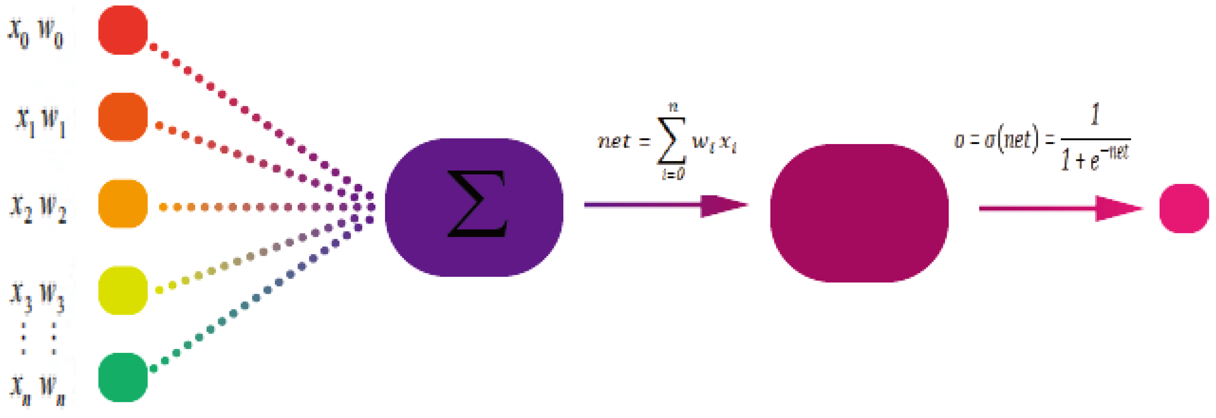
The LSTM-based exchange rate prediction model consists of an LSTM layer, dropout layer, and dense layer; the input of the model is the exchange rate data after data preprocessing. Through the LSTM neural network model, this model is first placed in an LSTM layer with 80 neural units and returns a 3D tensor; in order to avoid overfitting, a randomly ignored rate of 0.2 is then chosen. An LSTM layer with 100 neural units is used next, and a dropout layer with a ratio of 0.2 is added; finally, a network with one-dimensional output is defined by the dense layer. This model uses a dropout network in the LSTM layer, which prevents overfitting during model training, as it controls the random disconnection of some of the nodes connected to the neural network. The operational formula is given in Equation (9):

$$g=h^{*}·D\left(p\right)$$

(9)

where D stands for the operation of the dropout layer and p is an adjustable hyperparameter that indicates the value set for the ratio of disconnected neural network units in advance.

Because the dense layer can output the result as a number, it is suitable for problems of sequence prediction, and the final prediction is obtained through the dense output layer.

3.3.1. Description of the Time Distribution

According to the principle of maximum entropy, in the case of covariate transfer, the maximization of the shared knowledge of a time series can be achieved by finding the periods that are least similar to each other. This process is illustrated in Figure 5.

The time distribution describes this objective of segmenting the original time series by solving an optimization problem, which can be formulated as shown in Equation (10).

$$\begin{array}{cc}\underset{0<K\le K_0}{max}\hfill & \frac{\underset{n_1,\cdots ,n_K}{max}1}{K}\sum _{1\le i\ne j\le K}d\left(D_i,D_j\right)\hfill \\ \hfill & s.t.\forall i,{\Delta }_1<\left|D_i\right|<{\Delta }_2;\sum _i\left|D_i\right|=n\hfill \end{array}$$

(10)

where d is the distance unit, ${\Delta }_1$ and ${\Delta }_2$ are predefined parameters for avoiding very small values or very large values that may not capture distributional information, and $K_0$ is a hyperparameter for avoiding over-segmentation; d in Equation (10) can be an arbitrary distance function, e.g., Euclidean or some distributional-based distances, such as the MMD or KL difference.

The learning objective of the optimization problem is to maximize the difference between the average distributions of the cycles based on the determination of the value of K and the corresponding cycles so that the distributions of each cycle are as diverse as possible and the learned prediction model has a better generalization ability. The principle of segmentation can be explained in detail using the principle of maximum entropy [22]. First of all, it is necessary to find the most-different periods instead of the most-similar ones, and in the absence of prior assumptions about the segmentation of time series data, the entropy of the total distribution can only be maximized by diversifying the distribution of each period as much as possible so that a model can be built to flexibly cope with future data. At the same time, since there is no prior information about the data in the test set because the model is not visible during training, a more-reasonable approach is to train the model in the worst-case scenario, where different cycles can be simulated and the distributions of these cycles can be learned. If the model is able to learn from the worst-case scenario, then it will have a better ability to generalize to test data that it has never seen before. This assumption has also been validated in the theoretical analysis of time series models, as data diversity is very important in time series modeling.

In general, the time series segmentation optimization problem in Equation (10) is computationally very cumbersome and may not have a definite solution. However, by choosing a suitable distance metric, this optimization problem can be solved using dynamic programming. Because of the value of scalability in large-scale data and considering the goal of improving the efficiency as much as possible, a greedy algorithm can also be used to solve this optimization problem. Specifically, in order to more efficiently compute and avoid uncertain solutions, the actual exchange rate time series is divided into 10 equal parts, and each part must meet the minimum unit period. Subsequently, a value of k is randomly chosen from among the 10 segments, and each segment is of length ${\eta }_j$. In order to optimize the model, A and B are set as the beginning and the end of the time series, e.g., $k=2$, and one of the candidate segmentation points (denoted as C) is randomly chosen by maximizing the distributional variance $d(SAC,SCB)$. After determining C, the same method can be used to derive another point D when $k=3$. A similar method is applied for different values of k. Experiments have shown that this method can be used to select a more-appropriate segmentation period than that selected with the algorithm of random segmentation, and it has also been shown that the final performance of the predictive model deteriorates when k is very large or very small.

3.3.2. Time Distribution Matching

Based on the time series segments to be learned, a time series distribution matching module was designed to learn the common knowledge of the different periods by matching the distributions of the different periods, and this knowledge is used to match their distributions for the unknown sequences. As a result, the model trained in this step is able to generalize well to never-before-seen test sets in comparison with methods that rely only on local or statistical information. The structure is shown in Figure 6.

The loss function $\left(L_{pred}\right)$ for the prediction of time distribution matching can be formulated as in Equation (11):

$$L_{pred}\left(\theta \right)=\frac{1}{K}\sum _{j=1}^K\frac{1}{\left|D_j\right|}\sum _{i=1}^{\left|D_j\right|}l\left(y_i^j,M\left(x_i^j;\theta \right)\right)$$

(11)

where the pair $(x_i^j,y_i^j)$ denotes the i-th labeled segment from period $D_j$; L is a loss function, which can be a mean-squared error (MSE) loss function, and $\theta$ is a model parameter with learning capabilities.

Nonetheless, these steps can only cause the predictive knowledge for each period to be learned, and they cannot narrow down the diversity of distributions across different time periods in order to utilize their common knowledge. This problem can be solved using a simple approach, i.e., by employing some generalized distribution matching distances $\left(d\right(.),\dots ))$ as a regularization term to match the distributions of $D_i$ and $D_j$ in each period. In contrast to existing distribution matching methods, where the regularization term is often performed at a higher level, in this model, the regularization term is applied to the final output of the LSTM cellular units. $H={\left\{h^t\right\}}_{t=1}^V\in {\mathbb{R}}^{V\times q}$ is used to denote the hidden state V of the LSTM with feature dimension q. The pair $(D_i,D_j)$ of periodic distribution matching in the final hidden state can be expressed as in Equation (12):

$$L_{dm}\left(D_i,D_j;\theta \right)=d\left(h_i^v,h_j^v;\theta \right)$$

(12)

However, the above regularization term does not fully capture the time dependence of each hidden state in the LSTM network. Since each hidden state contains only part of the distributional information of the input sequence, each hidden state of the LSTM network should also be considered when constructing the distributional matching regularization term.

It can be seen in the temporal distribution matching schematic in Figure 6 that it is possible to capture the temporal dependency while matching the distributions of two LSTM cells. An importance vector is introduced so that the relative importance of the V hidden states inside the LSTM can be learned, and all of the hidden states are weighted with the normalized $\alpha$. Of course, for each pair of corresponding period segments, there is a corresponding $\alpha$. By doing so, the difference in the distribution of each pair of corresponding period segments can be dynamically reduced. Given a pair of period segments $(D_i,D_j)$, the loss of temporal distribution matching can be expressed as in Equation (13):

$$L_{tdm}\left(D_i,D_j;\theta \right)=\sum _{t=1}^v{\alpha }_{i,j}^{t}d\left(h_i^t,h_j^t;\theta \right)$$

(13)

where ${\alpha }_{i,j}^t$ denotes the similarity of the distribution between the $D_i$ period segments and the $D_j$ period segments for state t.

All hidden states in an LSTM network can be easily computed by following the standard LSTM computation. $\delta \left(.\right)$ denotes the computation of the next hidden state based on the previous state. The computation of this state can be formulated as Equation (14):

$$h_i^t=\delta \left(x_i^t,h_i^{t-1}\right)$$

(14)

The final goal of the time distribution matching is achieved with the computation defined in Equations (13) and (14):

$$L(\theta ,\alpha )=L_{pred}\left(\theta \right)+\lambda \frac{2}{K(K-1)}\sum _{i,j}^{i\ne j}{L}_{tdm}\left(D_i,D_j;\theta ,\alpha \right)$$

(15)

where $\lambda$ in Equation (15) is a hyperparameter used to balance the reduction in the prediction loss in training and the fitting of cycle pairs for migration learning; in addition, the average of the distributional differences in all corresponding cycle pairs is also calculated. To facilitate this calculation, small portions of $D_i$ and $D_j$ are selected to perform a forward operation in the recurrent neural network layer to concatenate all of the hidden features. Temporal distribution matching is then performed.

3.3.3. Learning on $\alpha$

A boosting-based importance assessment algorithm is used to learn $\alpha$ [23]. Prior to this, the network parameter $\theta$ is first pre-trained using all cycle-to-cycle data, i.e., using Equation (13). This is to train the model to be able to better characterize the hidden state to facilitate the learning of $\alpha$. In addition, by representing the pre-trained parameters as ${\theta }_0$, the importance of the hidden state can become progressively more realistic as the training progresses. Initially, for each LSTM layer, all weights are initialized to the same value, i.e., ${\alpha }_{i,j}={\left\{\frac{1}{V}\right\}}^V$. The difference in the distribution of the corresponding cycle pair is chosen as the indicator for boosting, and if the distribution difference in the ephemeral $n+1$ is larger than the distribution difference in the ephemeral n, we increase the value of ${\alpha }_{i,j}^{t,\left(n+1\right)}$ to reduce the distribution difference; otherwise, the value of ${\alpha }_{i,j}^{t,\left(n+1\right)}$ is kept unchanged. This can be expressed as in Equation (16):

$${\alpha }_{i,j}^{t,\left(n+1\right)}=\left\{\begin{array}{cc}{\alpha }_{i,j}^{t,\left(n\right)}\times G\left(d_{i,j}^{t,\left(n\right)},d_{i,j}^{t,\left(n-1\right)}\right)& d_{i,j}^{t,\left(n\right)}\ge d_{i,j}^{t,\left(n-1\right)}\\ {\alpha }_{i,j}^{t,\left(n\right)}& \mathrm{otherwise}\end{array}\right.$$

(16)

where $G\left(d_{i,j}^{t,\left(n\right)},d_{i,j}^{t,\left(n-1\right)}\right)$ can be expressed as in Equation (17):

$$G\left(d_{i,j}^{t,\left(n\right)},d_{i,j}^{t,(n-1)}\right)=\left(1+\sigma \left(d_{i,j}^{t,\left(n\right)}-d_{i,j}^{t,(n-1)}\right)\right)$$

(17)

The update function $G\left(d_{i,j}^{t,\left(n\right)},d_{i,j}^{t,\left(n-1\right)}\right)$ is computed with the distribution matching loss at different learning stages, while $d_{i,j}^{t,\left(n\right)}=D\left(h_i^t,h_j^t;{\alpha }_{i,j}^{t,\left(n\right)}\right)$ is the distribution difference at the t-th time step of the n-th period of iteration; $\sigma (.)$ is the sigmoid function. It is easy to see that $G(.)>1$; therefore, the proof’s importance increases again. Similar to the plain method, this can be simplified to Equation (18):

$${\alpha }_{i,j}^{t,(n+1)}=\frac{{\alpha }_{i,j}^{t,(n+1)}}{{\sum }_{j=1}^V{\alpha }_{i,j}^{t,(n+1)}}$$

(18)

Note that, by using Equations (16) and (18), the trained $\alpha$-value can be obtained.

4. Data Collection and Organization

Monthly data on the USD/CNY exchange rate published by the Wind database were selected, and these data were used as the basic data for this experiment; the style of the data series is shown in Figure 3. The exchange rate data released on this platform were the most-complete, and at the same time, the exchange price was accurate to the unit of minutes, so these data can meet the needs of researchers and investors in their study and analysis of short-term high-frequency exchange rate series in the international market. In this study, the real exchange rate price data from 2 January 2015 to 30 April 2022 were selected, and these data were split into training data and test data, respectively; each group of exchange rate price data contained 30,000 units, and the opening price was selected as the experimental object. The training data accounted for 80% of the total time series (24,000 articles), and the test data accounted for 20% of the total time series (a total of 6000 articles).

The main currency pair in Forex is the U.S. dollar currency pair. The U.S. dollar is currently the major currency in circulation in the world, occupying more than 80% of the global foreign exchange trading volume, which is mainly due to the United States of America’s economic strength, as it has a wide range of global trade as a result of its core position. The main reasons for this are as follows:

①

At present, almost all of the world’s national central banks use the dollar in foreign exchange reserves, although many countries’ central banks are currently reducing their proportions of foreign exchange reserves in dollars.

②

At present, the world’s major commodities, such as gold, are denominated in dollars. Therefore, global commodity transactions use them as a settlement currency, and borrowing and lending between countries are also denominated in U.S. dollars.

③

The U.S. dollar is the main medium of trade before cross-border transactions. The most-common example is that of oil, as oil is priced in dollars, so all international trade in oil must occur through the U.S. dollar.

④

Settlements of currency exchange rates between countries are all calculated through the dollar rate, and all other exchange rates are converted through the dollar.

Although USD/CNY was chosen as the research object in this study, the research results can be applied to other currencies.

The first step in the pre-construction of the neural network prediction model was that of data preprocessing, and among the various forms of methods used in the field of time series, the most widely used are normalization and standardization methods; the final prediction effect is different depending on the processing method used. Normalization and standardization methods can map time series data to a certain region, effectively reducing the time taken by a neural network to establish a construction process, but due to large gaps in the distributions of time series data, the prediction effect cannot be optimized, which is important for the realization of the task of the effective prediction of a time series through a neural network. In this study, a standardized method was used to preprocess the data, as defined in Equation (19):

$$x^{*}=\frac{x-x_{\mu }}{x_{\sigma }}$$

(19)

where $x^{*}$ is the normalized data, x is the original data, $x_{\sigma }$ is the standard deviation of the data, and $x_{\mu }$ is the mean of the data. The logical relationship between the processed data remained unchanged, and the results after the completion of the prediction were still standardized data, which needed to be back-normalized to obtain the actual size of the data.

5. Empirical Performance of the Model

In this section, we demonstrate the performance of the proposed model. First, we define the evaluation metrics used. Then, we present and discuss the obtained results.

5.1. Evaluation Indicators

In this study, the mean absolute percentage error (MAPE), root-mean-squared error (RMSE), and standard deviation (SD) were chosen as the evaluation indexes for the experiment. Smaller values of the MAPE, RMSE, and SD indicate a better prediction effect. Equations (20)–(22) represent the calculation of the MAPE, RMSE, and SD, respectively [24].

$$MAPE=\frac{1}{n}\sum _{i=1}^n\left|\frac{{\hat{y}}_i-y_i}{y_i}\right|\times 100\%$$

(20)

$$RMSE=\sqrt{\frac{1}{n}\sum _{i=1}^n{\left({\hat{y}}_i-y_i\right)}^2}$$

(21)

$$SD=\sqrt{\frac{1}{n}\sum _{i=1}^n{\left({\hat{y}}_i-y_i-\mu \right)}^2}$$

(22)

where n is the number of samples in the prediction result; ${\hat{y}}_i$ and $y_i$ are the predicted and real values of exchange rate fluctuation at the i-th moment, respectively; ${\hat{y}}_i-y_i$ is the error; and $\mu$ is the average error.

5.2. Empirical Process

In this work, EMD and SVR were realized using Python, and the neural network was built in the Keras environment. The accuracy of exchange rate series prediction was improved to reduce the discrepancies in the data. For this process, a six-step process was executed:

• Data acquisition: The data on the relevant exchange rate were downloaded from the Wind database and normalized.
• Residual sequence decomposition: The residual series (Res) was decomposed using the EMD algorithm to obtain n intrinsic modal components [IMF1, IMF2, …, IMFn] and the residual term $r_n$ to reduce the non-stationarity of exchange rate fluctuations.
• Prediction of IMF: The Res decomposition of the training set yielded n IMFs and one residual term $r_n$. For different frequencies of [IMF1, IMF2, …, IMFn], a residual term $r_n$ was established to train and predict the LSTM neural network, and the prediction results were used as the IMF and the residual terms of the residuals between the predicted value and the true value of the test set; then, they were summed to obtain the predicted value of the residuals of the test set $Y_{Res}$.
• LSTM neural network training and prediction: The exchange rate fluctuation data were divided into a training set and a test set; parameters such as the number of nodes in the hidden layer, the number of iterations, and the learning rate of LSTM were set according to experience; the neural network was trained using the training set. After the training was completed, the training set and test set were used to make respective predictions, and the training set’s prediction value ${\hat{Y}}_{train}$ and test set’s prediction value ${\hat{Y}}_{pre}$ were obtained. The residual sequence $s=Y_{true}-{\hat{Y}}_{train}$ of the training set’s prediction value and the true value were calculated, and $Y_{true}$ was taken as the true value of the exchange rate fluctuation.
• Prediction results: The prediction results of the combination model were the sum of the test set’s prediction value ${\hat{Y}}_{pre}$ and the test set’s residual prediction value $Y_{true}$, as shown in Equation (23).

  $$Y_{pre}={\hat{Y}}_{pre}-Y_{\mathrm{Re}s}$$

  (23)

The hyperparameters of the LSTM neural network were important factors that affected the accuracy of the model, but there was no rigorous and scientific formula for determining their size, but only empirical formulas summarized by scholars through a large number of experiments. In this study, the control variable method was used to find the optimal parameters of the LSTM neural network step by step, as shown in

Table 1. Model parameter setup.

Parameter	Parameter Value
Number of LSTM neural units in the first layer	100
Number of LSTM neural units in the second layer	120
Dropout parameters	0.1
Number of iterations	100
Batch size	64
Learning rate of the LSTM optimizer	0.001

.

5.3. EMD

The EMD results are shown in a schematic diagram in Figure 7, which shows the IMF and Res series obtained after the USD/CNY exchange rate was decomposed through EMD. As can be seen in the diagram, with the gradual progress of empirical modal decomposition, the originally complex and nonlinear series became simplified and, thus, easier to accurately predict [25].

The residuals of the fluctuations in the data on the exchange rate after the normalization process were decomposed through EMD to obtain six intrinsic modal components (IMF1–IMF6) and one residual component (Res), as shown in Figure 7, where IMF1 is the high-frequency portion, IMF7 is the low-frequency portion, and Res stands for the nonlinear trend. The first panel in Figure 7 shows the data before EMD; the following six panels are the intrinsic modal components (IMF1–IMF6) after decomposition; the last panel is the residual Res after decomposition.

5.4. Validation of the Model’s Smoothness

In order to determine the level of non-smoothness of the exchange rate series that was decomposed through EMD, the complexity of the series can be used as a criterion for the assessment of whether it is smooth or not, according to which the degree of non-smoothness of the original overall exchange rate series can be derived. Firstly, the complexity ($C_i$) of each IMF and Res was derived through entropy analysis, after which the exchange rate series was mapped onto the following phase space:

$$X_j=\left\{x_j,x_{j+1},\cdots ,x_{j+(m-1)}\right\}j=1,2,\cdots ,T-(m-1)$$

(24)

The small changes in the sequence due to noise were then represented as shown in Equation (25) using second-order differencing:

$$Z_j=\frac{\left({\Delta }^2{X}_j\right)}{\left|\overline{X_j}\right|}$$

(25)

Then, the entropy metric was derived:

$$C_i=-\sum _{g=1}^u{P}_{g}ln{P}_g$$

(26)

where $P_g$ is the probability distribution of group g and is satisfied by the following:

$$\sum _{g=1}^u{P}_g=1,u\le T-(m-1)$$

(27)

Finally, the complexity of each sub-sequence derived above was weighted and summed:

$$C_{EMD}=\sum _{i=1}^n{\omega }_i\times C_i$$

(28)

where $C_{EMD}$ is the complexity of EMD, $C_i$ is the complexity of the i-th sequence in EMD, and ${\omega }_i$ is the weight of the i-th sequence. If the complexity derived with the above method was lower than the complexity of the original sequence, this meant that the smoothness of the exchange rate sequence was improved [26].

5.5. Residual Prediction and Compensation

After the exchange rate sequence was processed through EMD, the complexity was reduced, and the problem of the non-smoothness and nonlinearity of the exchange rate sequence was effectively alleviated, which, in turn, reduced the difficulty of prediction.

After the establishment of an LSTM neural network model for the training and prediction of each IMF component, to obtain the prediction value of the IMF component of the test set, the residual prediction value of the test set was obtained by summing up the prediction values of all IMF components; according to Equation (8), the corresponding prediction result was added to the residual prediction value, and the compensation of the residuals was completed. The residual prediction results for the experimental data are shown in Figure 8. Due to the randomness and complexity of the residuals, it was difficult to predict them completely and accurately; they could only be predicted and compensated according to their overall trend, and Figure 8 shows this prediction effect.

5.6. Empirical Results of the Model

In order to better illustrate the superiority of the EMD-LSTM-SVR model in the prediction of exchange rate volatility, the trajectory prediction results and errors from a traditional BP neural network model and a single LSTM model are also provided.

As can be seen in Figure 9, all three models were able to predict the exchange rate fluctuations well on the whole. However, the BP neural network model performed poorly and was not as effective as the LSTM model and the EMD-LSTM-SVR model; the LSTM model was more stable than the BP model and had good results in forecasting; the EMD-LSTM-SVR model performed the best and was able to predict the longitude and latitude more accurately. More intuitive model error curves are shown in Figure 9 and Figure 10. The prediction results were statistically analyzed using the evaluation indexes, as shown in

Table 2. Comparison of the experimental results.

Evaluation Indicators	BP	LSTM	RNN	GRNN	EMD-LSTM-SVR
ME (10−4)	−2.211	−1.936	−2.26678	−1.88728	1.341
SD (10−4)	6.91	5.613	6.8718	5.52074	4.421
MAPE (%)	48.12	41.81	47.5576	40.9738	27.09
RMSE (10−4)	7.255	6.079	7.2099	5.95742	4.068

.

By analyzing Figure 9 and Figure 10 and Table 2, it can be seen that all five models had a good effect on the prediction of exchange rate fluctuations, though the EMD-LSTM-SVR model had the best performance. Selecting the data in Table 2 for a specific analysis, the EMD-LSTM-SVR model reduced the average absolute percentage error of the prediction results by 21.03% and 14.72% relative to the BP model and the LSTM model, and it improved the effect by 43.93% and 33.08%, respectively; the standard deviation was closer to the average error than that of the BP model and the LSTM model, which indicated that the EMD-LSTM-SVR model was more effective in predicting exchange rate fluctuations than the BP model and the LSTM model were. The EMD-LSTM-SVR model for exchange rate fluctuation prediction not only had a higher prediction accuracy, but it also ensured that most of the predicted positions deviated less from the actual positions.

6. Conclusions and Discussion

With a focus on exchange rate time series with non-stationary characteristics, the analysis and decomposition of a time series were used to reduce its complexity and, thus, improve the prediction accuracy. EMD was used to perform experiments; a sequence was first decomposed through EMD into several IMFs and a segment of signal Res components, and then, these segments were input into a previous LSTM model for exchange rates to train it for prediction. Next, these predictions were weighed and summed up; finally, in order to be more accurate, a layer of SVR was passed to reduce the noise and arrive at the final prediction value. The experimental results showed that the EMD-LSTM-SVR model for exchange rate fluctuation prediction not only had a high prediction accuracy, but it also ensured that most of the predicted positions deviated less from the actual positions.

Although this research on the prediction of actual exchange rates made some progress, there are still some deficiencies and areas for further study based on existing research: First, for the exchange rate forecasting model, the next step of research should be the comparison of the EMD-LSTM-SVR model with more time series forecasting models so as to better forecast exchange rates. Second, a set of empirical modal decompositions (EEMDs) should be used for the complexity reduction algorithm used on the exchange rate data sequence when performing forecasting experiments on the exchange rate, and EMD-based sequence decomposition should be used for a comparison of the complexity after the decomposition of the two algorithms in order to further improve the forecasting accuracy and increase the practical value.

The EMD algorithm can continuously decompose the original signal to obtain IMF components that meet certain conditions. These IMF components often have different frequencies, which provides a way of thinking about their use in the direction of harmonic detection. The EMD algorithm is widely used in the field of signal processing due to its orthogonality and convergence, but it does not have a fixed mathematical model like a wavelet analysis or neural network does, so some of its important properties have not been proven with careful mathematical methods. Moreover, the definition of the IMFs’ modal components has not been unified, and they can only be described using the connection between the zero point and the extreme value point of a signal, the local characteristics of a signal, etc. EMD still has a long way to go from theory to practical application, and the specific deficiencies of EMD are reflected in the following aspects:

• There is modal overlapping in IMF decomposition, that is to say, an IMF will contain feature components of different time scales. On the one hand, this is due to the signal itself, and on the other hand, this is a defect of the EMD algorithm itself.
• In the process of decomposing IMFs, many iterations are needed, and there is a lack of a standard for stopping the iterations, so IMFs obtained with different stopping conditions are different.

References

1. Hrmann, M. Liquidity Premia, Interest Rates and Exchange Rate Dynamics; Universitätsbibliothek Dortmund: Dortmund, Germany, 2011. [Google Scholar] [CrossRef]
2. Diebold, F.X.; Nerlove, M. The dynamics of exchange rate volatility: A multivariate latent factor ARCH model. J. Appl. Econom. 2010, 4, 1–21. [Google Scholar] [CrossRef]
3. Zhong, Y.; Shang, Y. Investigating Determinants of the CNY–CNH Exchange Rate Spread Using Extended GARCH Model. In Proceedings of the 2020 13th International Symposium on Computational Intelligence and Design (ISCID), Hangzhou, China, 12–13 December 2020; Volume 3, pp. 121–125. [Google Scholar] [CrossRef]
4. Chou, W.L. Exchange Rate Variability and China’s Exports. J. Comp. Econ. 2000, 28, 61–79. [Google Scholar] [CrossRef]
5. Tayyar, A.E. Political Exchange Rate Fluctuations Specific to Fixed Exchange Rate Regimes: A Case Study on Turkey. Ann. Econ. Ser. 2017, 2, 4–14. [Google Scholar]
6. Ouyang, A.Y.; Rajan, R.S. Real exchange rate fluctuations and the relative importance of nontradables. J. Int. Money Financ. 2015, 32, 5–15. [Google Scholar] [CrossRef]
7. Steurer, E.; Hann, T.H. Exchange rate forecasting comparison: Neural networks, symbolic machine learning and linear models. World Sci. 2024, 9, 175–190. [Google Scholar]
8. Maydybura, A.; Gohar, R.; Salman, A.; Wong, W.K.; Chang, B.H. The Asymmetric Effect of the Extreme Changes in the Economic Policy Uncertainty on the Exchange Rates: Evidence from Emerging Seven Countries. Ann. Financ. Econ. 2023, 18, 15–25. [Google Scholar] [CrossRef]
9. Dhamija, A.K.; Bhalla, V.K. Exchange rate forecasting: Comparison of various architectures of neural networks. Neural Comput. Appl. 2011, 20, 355–363. [Google Scholar] [CrossRef]
10. Dai, W. Research on Forecasting and Risk Measurement in Foreign Exchange Market Based on Deep Learning; Beijing University of Chemical Technology: Beijing, China, 2017. [Google Scholar]
11. Huang, J. Exchange rate prediction based on EEMD-LSTM model. Comput. Program. Ski. Maint. 2022, 17, 29–30. [Google Scholar] [CrossRef]
12. Lei, Z.; Shanghong, S.; Yue, W. Exchange rate prediction based on deep learning LSTM model. Stat. Decis. Mak. 2021, 37, 158–162. [Google Scholar] [CrossRef]
13. Choudhry, T. Interest rate, price level, and the inflation rate: Evidence from the UK during the gold standard regimes. Manch. Sch. 2024, 92, 20–39. [Google Scholar] [CrossRef]
14. Solis, P. Credit and Banking.Does the Exchange Rate Respond to Monetary Policy in Mexico? Solving an Exchange Rate Puzzle in Emerging Markets. J. Money Credit. Bank 2023, 2, 20–35. [Google Scholar] [CrossRef]
15. Hoa, T.V.; Anh, D.T.; Hieu, D.N. Foreign Exchange Rate Forecasting using Autoencoder and LSTM Networks. In Proceedings of the ICIIT’21: 2021 6th International Conference on Intelligent Information Technology, Ho Chi Minh, Vietnam, 25–28 February 2021. [Google Scholar] [CrossRef]
16. Sayed, I.A. Arima Model and forecasting of Exchange Rate of Bangladesh and Economic Dynamics. Indian J. Econ. Dev. 2014, 2, 3. [Google Scholar]
17. Greaves, J.G. Modeling with ARIMA-ARCH/GARCH Techniques to Estimate Weekly Exchange Rate of Liberia. Res. J. Financ. Account. 2018, 31, 78–102. [Google Scholar]
18. Hu, C.; Zheng, K.; Liu, L. Layered Exchange Rate Prediction Model Based on LSTM. In Proceedings of the ICMAI 2020: 2020 5th International Conference on Mathematics and Artificial Intelligence, Chengdu, China, 10–13 April 2020; Volume 22, pp. 16–35. [Google Scholar] [CrossRef]
19. Fu, C. Forecasting Exchange Rate with EMD-Based Support Vector Regression. In Proceedings of the 2010 International Conference on Management and Service Science, Wuhan, China, 24–26 August 2010; Volume 13, pp. 23–45. [Google Scholar] [CrossRef]
20. Tajdini, S.; Mehrara, M.; Taiebnia, A. Investigating the fluctuations of exchange rate based on monetary-behaviour approach. Int. J. Financ. Econ. IJFE 2023, 10, 12–35. [Google Scholar] [CrossRef]
21. Aminian, G.; Abroshan, M.; Khalili, M.M.; Toni, L.; Rodrigues, M.R.D. An Information-theoretical Approach to Semi-supervised Learning under Covariate-shift. arXiv 2022, arXiv:2202.12123. [Google Scholar] [CrossRef]
22. Deng, J.; Pandey, M. Optimal maximum entropy quantile function for fractional probability weighted moments and its applications in reliability analysis. Appl. Math. Model. 2023, 32, 15–25. [Google Scholar] [CrossRef]
23. Giutini, R.; Gaudette, K. Remanufacturing: The next great opportunity for boosting US productivity. Bus. Horizons 2003, 46, 41–48. [Google Scholar] [CrossRef]
24. Wen, J.; Fang, X.; Cui, J.; Fei, L.; Yan, K.; Chen, Y.; Xu, Y. Robust sparse linear discriminant analysis. IEEE Trans. Circuits Syst. Video Technol. 2019, 29, 390–403. [Google Scholar] [CrossRef]
25. Wen, J.; Xu, Y.; Liu, H. Incomplete multiview spectral clustering with adaptive graph learning. IEEE Trans. Cybern. 2020, 50, 1418–1429. [Google Scholar] [CrossRef] [PubMed]
26. Wen, J.; Xu, Y.; Li, Z.; Ma, Z.; Xu, y. Inter-class sparsity based discriminative least square regression. Neural Netw. 2018, 102, 36–47. [Google Scholar] [CrossRef] [PubMed]
Figure 1. The main components of a sigmoid layer.
Mathematics 12 00614 g001
Figure 2. The structure of an LSTM neural network.
Mathematics 12 00614 g002
Figure 3. Non-stationarity of exchange rate fluctuations.
Mathematics 12 00614 g003
Figure 4. The structure of the proposed EMD-LSTM-SVR model.
Mathematics 12 00614 g004
Figure 5. Illustration of the time distribution.
Mathematics 12 00614 g005
Figure 6. Schematic diagram of time distribution matching.
Mathematics 12 00614 g006
Figure 7. Schematic diagram of the EMD results.
Mathematics 12 00614 g007
Figure 8. Residual forecasts of exchange rate fluctuations.
Mathematics 12 00614 g008
Figure 9. Forecast of exchange rate fluctuations.
Mathematics 12 00614 g009
Figure 10. Plot of model error fluctuations.
Mathematics 12 00614 g010