Assessment of the Overall Lifetime Performance Index of Weibull Products in Multiple Production Lines

Abstract

Process capability indices have been extensively employed to assess process performance in order to drive ongoing enhancements in quality and productivity, where the larger, the better for these lifetime performance indices. For multiple production lines, an overall lifetime performance index is proposed and the relationship between the overall lifetime performance index and the individual lifetime performance index is displayed. For products with lifetimes following the Weibull distribution for the ith production line, the maximum likelihood estimator and asymptotic distribution for the individual lifetime performance index were investigated so that the maximum likelihood estimator and asymptotic distribution for the overall lifetime performance index were also derived. Based on the pre-assigned target value of the overall lifetime performance index, the target value of an individual lifetime performance index could be determined. To test whether the overall lifetime performance index reached the target value was equivalent to testing whether the individual lifetime performance index reached the corresponding target value. The testing procedure based on the maximum likelihood estimator is given in this paper and the analysis of test power is displayed by figures. Finally, one practical example is given to illustrate the use of this testing algorithmic procedure to determine whether the overall production process was capable.

1. Introduction

In this study, we investigated the lifetimes of components in multiple production lines, focusing on the “larger-the-better” property exhibited by product lifetimes. Specifically, we utilized the lifetime performance index C_L introduced by Montgomery [1] with unilateral tolerance. While many process capability indices (PCIs) typically assume a normal distribution for quality characteristics, product lifetimes often adhere to distributions such as exponential, gamma, or Weibull distributions (refer to Anderson et al. [2], Meyer [3], and Epstein and Sobel [4]). Here, we presumed a Weibull distribution for the lifetime of the products. Since a larger lifetime of products is desired, the lifetime performance index recommended by Montgomery [1] was used in this study.

For products produced in a single production line, Tong et al. [5] developed the uniformly minimum variance unbiased estimator for the index of C_L and established a hypothesis-testing procedure that assumes a one-parameter exponential distribution for the complete sample. However, in real-world scenarios, experimenters might not always have the ability to observe the lifetimes of all tested items due to constraints, such as time limitations, financial and material resources, negligence of typists or recorders, and mechanical or experimental challenges. Consequently, incomplete data, such as progressive censoring data, may be collected (see Aggarwala [6], Balakrishnan and Aggarwala [7], Hong et al. [8], Wu et al. [9], Sanjel and Balakrishnan [10], and Lee et al. [11]). In the context of step-stress-accelerated life-testing data, Lee et al. [12] evaluated the lifetime performance index for exponential products. For the progressive type I interval censored sample, the testing procedure for the lifetime of a product following a Weibull distribution in a single production line was proposed by Wu and Lin [13]. The experimental design for this testing procedure to reach a given test power or minimize the total experimental cost for Weibull products was proposed by Wu et al. [14]. The sampling design to minimize the total experimental cost for Chen products was developed by Wu and Song [15].

We focused on the case of progressive type I interval censoring. The censoring scheme is outlined as follows: Assume that n products are subjected to a life test starting at time 0. Let the predefined inspection times be (t₁, …, t_m), where t_m is the termination time of the experiment. Thus, there are m inspection intervals in this life test. At the ith time point, we observe X_i failed units in the ith time interval (t_i−1, t_i) and then R_i products are removed from the remaining products. Keep doing the same process until we observe X_m failed units in the last time interval (t_m−1, t_m) and the remaining products are removed. Then, the experiment is terminated at the time point t_m and we collect the observed progressive type I interval censored sample (X₁, …, X_m) under the censoring scheme of (R₁, …, R_m).

For products produced in multiple production lines with lifetimes following Weibull distributions, an overall lifetime performance index was proposed in this study. We used the maximum likelihood estimator for the lifetime performance index as the test statistic to test whether the overall lifetime performance index attained the desired target level for the progressive type I interval censored sample. For the estimation method of maximum likelihood estimators, Wang et al. [16] found the maximum likelihood estimators of the parameters of the inverse Gaussian distribution using maximum rank set sampling with unequal samples. Phaphan et al. [17] investigated the maximum likelihood estimation of the weighted mixture generalized gamma distribution.

The remainder of this paper is structured as follows: In Section 2, the overall lifetime performance index is developed for products produced in multiple production lines and the connection with the conforming rate, the overall lifetime performance index, and the individual lifetime performance index is elucidated. Section 3.1 presents the derivation of the maximum likelihood estimator and the asymptotic distribution of both the overall and individual lifetime performance indices based on a progressive type I interval censored sample, assuming a Weibull distribution. In Section 3.2, the testing procedure for the overall lifetime performance index involving all individual lifetime performance indices is proposed. The impacts of various parameter configurations, especially the number of production lines on the test power, are studied in this section as well. Section 3.3 provides a numerical example to illustrate the proposed testing procedure. The conclusive findings are summarized in Section 4.

2. The Overall Lifetime Performance Index and the Conforming Rate

Suppose that there are d production lines producing products. The lifetime U_i of products in the ith production line has a Weibull distribution with the probability density function (PDF), cumulative distribution function (CDF), and hazard function (HF) as follows:

$$f_{U_i}\left(u\right)=\frac{{\delta }_i}{{\lambda }_i}{\left(\frac{u}{{\lambda }_i}\right)}^{{\delta }_i-1}\mathit{exp}\left\{-{\left(\frac{u}{{\lambda }_i}\right)}^{{\delta }_i}\right\},u>0,{\delta }_i>0,{\lambda }_i>0,$$

(1)

$$F_{U_i}\left(u\right)=1-\mathit{exp}\left\{-{\left(\frac{u}{{\lambda }_i}\right)}^{{\delta }_i}\right\},u>0,{\delta }_i>0,{\lambda }_i>0$$

(2)

and

$$h\left(u\right)=\frac{f_{U_i}\left(u\right)}{1-F_{U_i}\left(u\right)}=\frac{{\delta }_i}{{\lambda }_i}{\left(\frac{u}{{\lambda }_i}\right)}^{{\delta }_i-1},$$

(3)

where ${\lambda }_i$ is the scale parameter and δ_i is the shape parameter, i = 1, …, d. The Weibull distribution is a continuous probability distribution that is commonly used to model the distribution of lifetimes or survival times. If δ_i > 1, the HF has a bathtub shape; if δ_i < 1, the HF initially decreases and then increases over time; if δ_i = 1, the HF is constant over time, resulting in a constant failure rate (exponentially distributed failure times). Montgomery [1] proposed a larger-the-better type process capability index C_L given as

$$C_L=\frac{\mu -L}{\sigma },$$

(4)

where μ denotes the process mean, σ denotes the process standard deviation, and L is the specified lower specification limit. This index is also called the lifetime performance index for products. Consider the transformation of $Y_i={U_i}^{{\delta }_i}$ with $k_i=\frac{1}{{{\lambda }_i}^{{\delta }_i}}$; then, the new lifetime Y_i follows a one-parameter exponential distribution with PDF and CDF as follows:

$$f_{Y_i}\left(y\right)=k_i\mathit{exp}\left\{-k_{i}y\right\},\hspace{1em}y>0,k_i>0,$$

(5)

$$F_{Y_i}\left(y\right)=1-exp\left(-k_{i}y\right),\hspace{1em}y>0,k_i>0.$$

(6)

The mean and standard deviation of the new lifetime of products are obtained using ${\mu }_i=E\left(Y_i\right)=\frac{1}{k_i}$ and ${ \sigma }_i=\sqrt{Var\left(Y_i\right)}=\frac{1}{k_i}$. The lifetime performance index for the ith production line can be written as

$$C_{L_i}=\frac{{\mu }_i-L_i}{{ \sigma }_i}=\frac{\frac{1}{k_i}-L_i}{\frac{1}{k_i}}=1-k_i{L}_i.$$

(7)

The lifetime performance index $C_{L_i}$ can accurately assess the lifetime performance of products since the smaller the failure rate k_i, the larger the lifetime performance index $C_{L_i}$.

The conforming rate for the ith production line denoted by $P_{r_i}$ is defined as the probability of the lifetime of an item of a product that exceeds the lower specification limit (i.e., $Y_i\ge L_i$) and it can be obtained using

$$P_{r_i}=P\left(Y_i\ge L_i\right)={\int }_{L_i}^{\infty }{k}_i{e}^{-k_{i}y}dy=e^{-k_i{L}_i }=e^{C_{L_i}-1},-\infty <C_{L_i}<1.$$

(8)

Apparently, the conforming rate for the ith production line is an increasing function of the lifetime performance index $C_{L_i}$. If the engineer wishes $P_{r_i}$ to exceed 0.818731, then they can obtain the value of $C_{L_i}$ that exceeds 0.8 from Equation (8).

We assumed that there are d independent production lines for products. The overall conforming rate denoted by P_r can be obtained using

$$P_r=P\left(Y_i\ge L_i,i=1,\cdots ,d\right)=\mathit{exp}\left\{-\sum _{i=1}^d{k}_i{L}_i\right\}=\mathit{exp}\left\{\sum _{i=1}^d{C}_{L_i}-d\right\},-\infty <C_{L_i}<1.$$

Denote the overall lifetime performance index as C_T, which satisfies

$$P_r=exp\left\{{\sum }_{i=1}^d{C}_{L_i}-d\right\}=exp\left\{C_T-1\right\},-\infty <C_T<1.$$

(9)

From Equation (9), it is observed that C_T is an increasing function of P_r. Solving this equation, we obtained the following equation:

$$C_T=\sum _{i=1}^d{C}_{L_i}-\left(d-1\right),-\infty <C_T<1.$$

(10)

We considered a reasonable setup of equal individual lifetime performance indices as $C_{L_1}=\cdots =C_{L_d}=C_L$. Solving Equation (10), we obtained

$$C_L=\frac{C_T+d-1}{d},-\infty <C_T<1.$$

(11)

If the engineer sets the desired overall lifetime performance index to be C_T = c₀, the individual lifetime performance index for each production line C_L can be determined as $C_L=\frac{c_0+d-1}{d}$ using Equation (11). For example, the experimenter wants to have the overall conforming rate as P_r = 0.9512. We can find C_T = 0.95 from Equation (9) and then the desired level for each production line can be found from Equation (11) as C_L = 0.9750, 0.9833, 0.9875, 0.9900, 0.9917, 0.9929, 0.9938, 0.9944, and 0.9950 for d = 2, 3, …, 10.

3. The Testing Procedure for the Overall Lifetime Performance Index

In this section, the maximum likelihood estimator and the asymmetric distribution of each lifetime performance index and the overall lifetime performance index are derived in Section 3.1. The testing procedure for testing whether the overall lifetime performance index reaches the desired target level and the power analysis are given in Section 3.2. In Section 3.3, one numerical example is given to illustrate our proposed testing procedure.

3.1. Maximum Likelihood Estimator of the Lifetime Performance Index

For the ith production line, we collect the progressive type I interval censored sample as $X_{i1},\dots ,X_{im}$ at the observation time points $t_1,\dots ,t_m$. For this type of censored sample $X_{i1},\dots ,X_{im}$, the likelihood function is obtained as

$$L\left(k_i\right)\propto \prod _{j=1}^m{\left(F\left(t_j\right)-F\left(t_{j-1}\right)\right)}^{x_{ij}}{\left(1-F\left(t_j\right)\right)}^{R_{ij}}$$

$$\propto \prod _{j=1}^m{\left(1-e^{-k_i(y_{ij}-y_{i(j-1)}) }\right)}^{x_{ij}}{e}^{-k_i\left(y_{i\left(j-1\right)}{x}_{ij}+y_{ij}{R}_{ij}\right)},$$

(12)

where $y_{ij}=t_j^{{\delta }_i}$; j = 1, $\cdots$, m; and i = 1,$\cdots$, d. The log-likelihood function is

$$logL\left(k_i\right)\propto \sum _{j=1}^m\left\{x_{ij}\mathit{log}\left(1-e^{-k_i\left(y_{ij}-y_{i\left(j-1\right)}\right)}\right)-k_i\left(y_{i\left(j-1\right)}{x}_{ij}+y_{ij}{R}_{ij}\right)\right\}.$$

(13)

From Casella and Berger [18], taking the derivative of the above log-likelihood function with respect to parameter k_i and equating to zero, we have the following log-likelihood equation:

$$\frac{d}{d{k}_i}logL\left(k_i\right)=\sum _{j=1}^m\left\{x_{ij}\frac{\left(y_{ij}-y_{i\left(j-1\right)}\right)e^{-k_i\left(y_{ij}-y_{i\left(j-1\right)}\right)}}{1-e^{-k_i\left(y_{ij}-y_{i\left(j-1\right)}\right)}}-\left(y_{i\left(j-1\right)}{x}_{ij}+y_{ij}{R}_{ij}\right)\right\}=0.$$

(14)

The maximum likelihood estimator of k_i can be obtained by solving Equation (14) numerically and it is denoted by ${\widehat{k}}_i$.

In order to obtain the asymptotic variance of the distribution of the maximum likelihood estimator, we need to find the Fisher’s information number, which is $I_i\left(k_i\right)=-E\left[\frac{d^2\mathit{log}L\left(k_i\right)}{d{k}_i^2}\right]$ (see Casella and Berger [18]). We need to find the second derivative as follows:

$$\frac{d^2\mathit{log}L\left(k_i\right)}{d{k}_i^2}$$

$$=\sum _{j=1}^m\left\{x_{ij}\frac{-{\left(y_{ij}-y_{i\left(j-1\right)}\right)}^2{e}^{-k_i\left(y_{ij}-y_{i\left(j-1\right)}\right)}\left(1-e^{-k_i\left(y_{ij}-y_{i\left(j-1\right)}\right)}\right)-{\left(y_{ij}-y_{i\left(j-1\right)}\right)}^2{e}^{-2k_i\left(y_{ij}-y_{i\left(j-1\right)}\right)}}{{\left(1-e^{-k_i\left(y_{ij}-y_{i\left(j-1\right)}\right)}\right)}^2}\right\}$$

$$=\sum _{j=1}^m\left\{x_{ij}\frac{-{\left(y_{ij}-y_{i\left(j-1\right)}\right)}^2{e}^{-k_i\left(y_{ij}-y_{i\left(j-1\right)}\right)}}{{\left(1-e^{-k_i\left(y_{ij}-y_{i\left(j-1\right)}\right)}\right)}^2}\right\}.$$

(15)

It is observed that

$$\left.X_{ij}\right|X_{i(j-1)},\dots ,X_{i1}~\mathrm{Binomial}\left(n-{\displaystyle \sum _{l=1}^{j-1}{X}_{il}},q_{ij}\right),$$

(16)

where $q_{ij}=\frac{\left.F{\left(t\right.}_j)-F{\left(t\right.}_{j-1}\right)}{\left.1-F{\left(t\right.}_{j-1}\right)}=1-e^{-k_i\left(y_{ij}-y_{i\left(j-1\right)}\right)},j=1,\cdots ,m$.

Hence, we have

$$E\left(\left.X_{ij}\right|X_{i(j-1)},\cdots ,X_{i1},R_{i,j-1},\cdots ,R_{i1}\right)=n{q}_{ij}{\displaystyle \prod _{l=1}^{j-1}\left(1-p_l\right)\left(1-q_{il}\right)},j=1,\dots ,m.$$

(17)

Therefore, the Fisher’s information number will be

$$I_i\left(k_i\right)$$

$$=-E\left(\sum _{j=1}^m{x}_{ij}\frac{-\frac{1}{k_i^2}\left(1-q_{ij}\right){log}^2\left(1-q_{ij}\right)}{q_{ij}^2} \right)=\frac{n}{k_i^2}\sum _{j=1}^m\frac{{log}^2\left(1-q_{ij}\right)}{q_{ij}} \prod _{l=1}^{j-1}\left(1-p_{il}\right)\left(1-q_{il}\right),$$

(18)

The asymptotic variance is denoted as ${V_i\left({\widehat{k}}_i\right)=I}_i^{-1}\left({\widehat{k}}_i\right)$. Then, we have ${\widehat{k}}_i\underset{n\to \mathrm{\infty }}{\stackrel{d}{\to }}N\left(k_i,I_i^{-1}\left({\widehat{k}}_i\right)\right)$.

As a special case, we considered equal interval lengths where $t_j-t_{j-1}=t$ and $q_{ij}=1-e^{-k_i\left(y_{ij}-y_{i\left(j-1\right)}\right)}=1-e^{-k_i\left({\left(jt\right)}^{\delta }-{\left(\right(j-1\left)t\right)}^{\delta }\right)},j=1,\cdots ,m$. We also considered p_j = p, $j=1,\cdots ,m$. Equation (14) can be simplified to

$$\sum _{j=1}^m\left[x_{ij}\frac{\left[{\left(jt\right)}^{{\delta }_i}-{\left(\left(j-1\right)t\right)}^{{\delta }_i}\right]\mathit{exp}\left\{-k_i\left[{\left(jt\right)}^{{\delta }_i}-{\left(\left(j-1\right)t\right)}^{{\delta }_i}\right]\right\}}{1-\mathit{exp}\left\{-k_i\left[{\left(jt\right)}^{{\delta }_i}-{\left(\left(j-1\right)t\right)}^{{\delta }_i}\right]\right\}}-\left({\left[\left(j-1\right)t\right]}^{{\delta }_i}{x}_{ij}+{\left(jt\right)}^{{\delta }_i}{R}_{ij}\right)\right]=0.$$

(19)

Solving for k_i numerically, we can obtain the maximum likelihood estimator for k_i denoted by ${\widehat{k}}_i$. Furthermore, the asymptotic variance of ${\widehat{k}}_i$ can be expressed as

$$V\left({\widehat{k}}_i\right)=I_i^{-1}\left({\widehat{k}}_i\right)=\frac{k_i^2}{n}{\left[\sum _{j=1}^m\frac{{\mathit{log}}^2\left(1-q_{ij}\right)}{q_{ij}}\prod _{l=1}^{j-1}\left(1-p_l\right)\left(1-q_{il}\right)\right]}^{-1}.$$

(20)

From Casella and Berger [18], by the property of the invariance of the maximum likelihood estimator, the maximum likelihood estimator of $C_{L_i}$ can be obtained using

$${\widehat{C}}_{L_i}=1-{\widehat{k}}_i{L}_i.$$

(21)

The delta method in Casella and Berger [18] is a technique in statistics that allows us to approximate the distribution of a function of random variables using the first-order Taylor expansion. Making use of the Delta method, we can show that

$${\widehat{C}}_{L_i}\underset{n\to \infty }{\stackrel{d}{\to }}N\left(C_{L_i},V\left({\widehat{C}}_{L_i}\right)\right),$$

(22)

where $V\left({\widehat{C}}_{L_i}\right)={L_i}^{2}V\left({\widehat{k}}_i\right)$.

Using the property of the invariance of the maximum likelihood estimator, the maximum likelihood estimator of C_T is

$${\widehat{C}}_T=\sum _{i=1}^d{\widehat{C}}_{L_i}-\left(d-1\right).$$

(23)

Its asymptotic distribution is ${\widehat{C}}_T\underset{n\to \mathrm{\infty }}{\stackrel{d}{\to }}N\left(C_T,\sum _{i=1}^d\widehat{V}\left({\widehat{C}}_{L_i}\right)\right),$ where the variance of ${\widehat{C}}_T$ is ${\sum }_{i=1}^{d}V\left({\widehat{C}}_{Li}\right)$ and its estimate is ${\sum }_{i=1}^d\widehat{V}\left({\widehat{C}}_{Li}\right)$.

3.2. The Testing Procedure for the Overall Lifetime Performance Index and Power Analysis

For the assessment of whether the overall lifetime performance index exceeds the desired target value c₀, we develop a statistical testing procedure in this section. The null and alternative hypotheses are $H_0: C_T\le c_0$ (d production lines are not capable) vs. $H_a: C_T>c_0$ (d production lines are capable). Under the condition of $C_{L_1}=\cdots =C_{L_d}=C_L$, if the overall lifetime performance index $C_T=\sum _{i=1}^d{C}_{L_i}-\left(d-1\right)>c_0$, we can obtain the condition of $C_{L_i}>c_0^{*}, i=1,\dots ,d$, where $c_0^{*}$ is the target value for each lifetime performance index according to $c_0^{*}=\frac{c_0+d-1}{d}$. The above statistical hypothesis for testing the overall lifetime performance index can be equivalently set up as follows.

$H_0:C_{L_i}\le c_0^{*} \mathrm{for}\mathrm{some}i \left(d\mathrm{production}\mathrm{lines}\mathrm{are}\mathrm{not}\mathrm{capable}\right)$ vs. $H_a:C_{L_i}>c_0^{*},i=1,\cdots ,d$ (d production lines are capable). This is the so-called intersection–union test in Casella and Berger [18]. For the ith test of $H_{0i}:C_{L_i}\le c_0^{*}$ and $H_{ai}:C_{L_i}>c_0^{*}$, the maximum likelihood estimator of $C_{L_i}$ denoted by ${\widehat{C}}_{L_i}$ is used as the test statistic and the critical value $C_{L_i}^0$ is determined using $C_{L_i}^0=1-(Z_{1-{\alpha }^{\prime }}\sqrt{I_i^{-1}(k_{i0})}+k_{i0})L_i$ under the size of α’ = α^1/d (see Wu and Lin [13]). The rejection region for this test is $R_i=\left\{{\widehat{C}}_{L_i}|{\widehat{C}}_{L_i}>C_{L_i}^0\right\}.$ To test $H_0:C_{L_i}\le c_0^{*} \mathrm{for}\mathrm{some}i$ vs. $H_a:C_{L_i}>c_0^{*},i=1,\cdots ,d,$ the overall rejection region is determined using $R=\bigcap _{i=1}^d{R}_i=\bigcap _{i=1}^d\left\{{\widehat{C}}_{L_i} | {\widehat{C}}_{L_i}>C_{L_i}^0\right\}$ such that the size of this test is still α.

Following the Algorithm 1, algorithm of the testing procedure for $C_T,$ the testing procedure was implemented as follows.

Algorithm 1: Testing procedure for $C_T.$

1: Given a known lower specification Li, observe the progressive type I interval censored sample $X_{i1},\dots ,X_{im}$ at the pre-set time points $t_1,\dots ,t_m$ with censoring schemes of $R_1,\dots ,R_m$ from the Weibull distribution. 2: Determine the required level $c_0$ to achieve a pre-assigned conforming rate Pr from Equation (9) and then determine the required level $c_0^{*}$ for each production line. Then, the testing hypothesis $H_0:C_{L_i}\le c_0^{*}\mathrm{for}\mathrm{some}i$ vs. $H_a:C_{L_i}>c_0^{*},i=1,\cdots ,d$ is constructed. 3: Obtain the value of the test statistic ${\widehat{C}}_{L_i}$. 4: For the level of significance α, we can calculate the critical value $C_{L_i}^0=1-\left(Z_{1-{\alpha }^{\prime }}\sqrt{I_i^{-1}\left(k_{i0}\right)}+k_{i0}\right)L_i$, where $k_{i0}=\frac{1-c_0^{*}}{L_i}$, α’ = α1/d, and $I_i^{-1}\left(k_{i0}\right)$ is defined in Equation (18). 5: The decision rule is to conclude that the overall lifetime performance index of the products exceeds the required level if ${\widehat{C}}_{L_i}>C_{L_i}^0$ for $i=1,\dots ,d$ holds.

Furthermore, the test power function h(c₁) of the testing procedure at the point of $C_T=d{C}_L-\left(d-1\right)=c_1>c_0$ or $C_L=\frac{c_1+d-1}{d}=c_1^{*}$ can be obtained as follows:

$$h\left(c_1\right)=P\left({\widehat{C}}_{Li}>C_{Li}^0,i=1,\cdots ,d |{ c}_1^{*}=1-k_{i1}{L}_i,i=1,\cdots ,d\right)$$

$$=P\left(\left.1-{\widehat{k}}_i{L}_i>1-\left(Z_{1-{\alpha }^{\prime }}\sqrt{{I_i}^{-1}\left(k_{i0}\right)}+k_{i0}\right)L_i,i=1,\cdots ,d\right|k_{i1}=\frac{1-c_1^{*}}{L_i},k_{i0}=\frac{1-c_0^{*}}{L_i},i=1,\cdots ,d\right)$$

$$=P\left(\left.{\widehat{k}}_i<k_{i0}+Z_{1-{\alpha }^{\prime }}\sqrt{{I_i}^{-1}\left(k_{i0}\right)},i=1,\cdots ,d\right|k_{i1}=\frac{1-c_1^{*}}{L_i},k_{i0}=\frac{1-c_0^{*}}{L_i},i=1,\cdots ,d\right)$$

$$={\displaystyle \prod _{i=1}^{d}P\left(\left.{\widehat{k}}_i<k_{i0}+Z_{1-{\alpha }^{\prime }}\sqrt{{I_i}^{-1}\left(k_{i0}\right)}\right|k_{i1}=\frac{1-c_1^{*}}{L_i},k_{i0}=\frac{1-c_0^{*}}{L_i}\right)}$$

$$={\displaystyle \prod _{i=1}^{d}P\left(\left.\frac{{\widehat{k}}_i-k_{i1}}{\sqrt{{I_i}^{-1}\left(k_{i1}\right)}}<\frac{k_{i0}-k_{i1}+Z_{1-{\alpha }^{\prime }}\sqrt{{I_i}^{-1}\left(k_{i0}\right)}}{\sqrt{{I_i}^{-1}\left(k_{i1}\right)}}\right|k_{i1}=\frac{1-c_1^{*}}{L_i},k_{i0}=\frac{1-c_0^{*}}{L_i}\right)}$$

$$={\displaystyle \prod _{i=1}^d\left(\Phi \left(\left.\frac{k_{i0}-k_{i1}+Z_{1-{\alpha }^{\prime }}\sqrt{I^{-1}\left(k_{i0}\right)}}{\sqrt{{I_i}^{-1}\left(k_{i1}\right)}}\right|k_{i1}=\frac{1-c_1^{*}}{L_i},k_{i0}=\frac{1-c_0^{*}}{L_i}\right)\right)},$$

(24)

where $\Phi \left(\cdot \right)$ is the CDF for the standard normal distribution, $k_{i1}=\frac{1-c_1^{*}}{L_i}$, $k_{i0}=\frac{1-c_0^{*}}{L_i}$, and $i=1,\cdots ,d$.

Under L₁ = … = L_d = L, the power function is reduced to

$$h\left(c_1\right)={\displaystyle \prod _{i=1}^d\left(\Phi \left(\left.\frac{k_0-k_1+Z_{1-{\alpha }^{\prime }}\sqrt{{I_i}^{-1}\left(k_0\right)}}{\sqrt{{I_i}^{-1}\left(k_1\right)}}\right|k_1=\frac{1-c_1^{*}}{L},k_0=\frac{1-c_0^{*}}{L}\right)\right)}$$

The powers h(c₁) for testing $H_0:C_T\le 0.8$ are tabulated in Table A1, Table A2, Table A3, Table A4, Table A5, Table A6, Table A7, Table A8 and Table A9 for d = 2, 3, and 4, with α = 0.050, 0.075, and 0.100, respectively, where c₁ = 0.850, 0.875, 0.885, 0.900, 0.930, 0.960; m = 5, 6, and 7; n = 30, 50, and 70; p = 0.050, 0.075, and 0.100; L = 0.05; and T = 0.5. The power values $h\left(c_1\right)$ are showcased in Figure 1, Figure 2, Figure 3, Figure 4 and Figure 5 to exemplify several standard cases. We obtained the following findings: (1) From Figure 1, the power increased when n increased for fixed d = 2, α = 0.05, m = 5, and p = 0.05 (other combinations of d, m, p, and α also showed the same pattern); (2) from Figure 2, the power increased when m increased for fixed d = 2, n = 30, p = 0.05, and α = 0.05 (other combinations of d, n, p, and α also showed the same pattern); (3) from Figure 3, the power increased when p increased for fixed d = 2, n = 30, m = 5, and α = 0.05 (other combinations of d, n, m, and α also had the same pattern); (4) from Figure 4, the power increased when α increased under d = 2, n = 30, m = 5, and p = 0.05 (other combinations of d, n, m, and p also had the same pattern); (5) from Figure 5, the power increased when d increased under n = 30, m = 5, p = 0.05, and α = 0.05 (other combinations of n, m, p, and α also had the same pattern); (6) from Figure 1, Figure 2, Figure 3, Figure 4 and Figure 5, the power increased when the value of c₁ increased for any combination of d, n, m, p, and α.

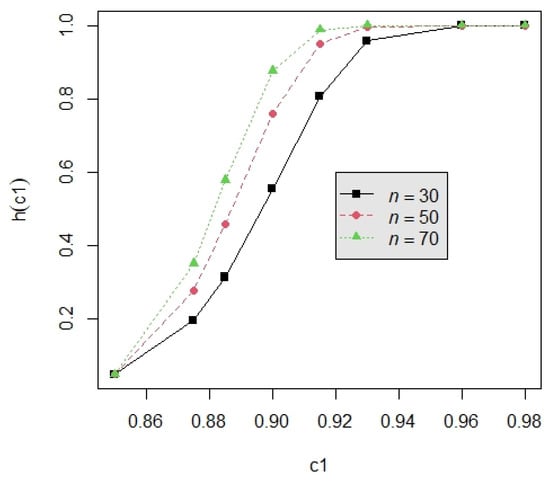
Figure 1. The power curve for d = 2; α = 0.05; m = 5; p = 0.05; and n = 30, 50, and 70.

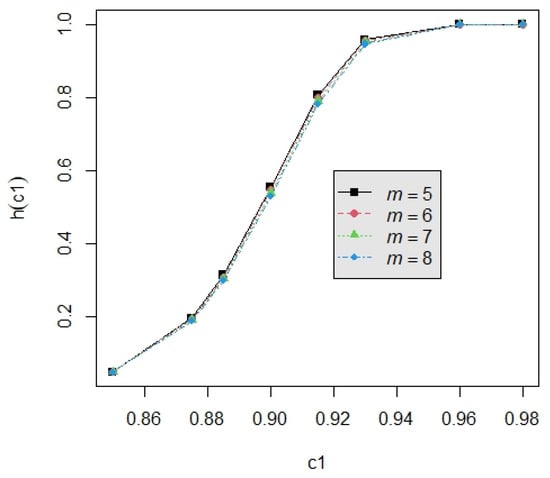
Figure 2. The power curve for d = 2; α = 0.05; n = 30; p = 0.05; and m = 5, 6, 7, and 8.

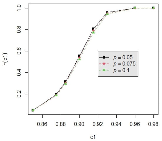
Figure 3. The power curve for d = 2; α = 0.05; n = 30; m = 5; and p = 0.050, 0.075, and 0.100.

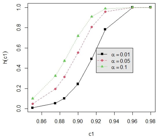
Figure 4. The power curve for d = 2; n = 30; m = 5; p = 0.05; and α = 0.01, 0.05, and 0.10.

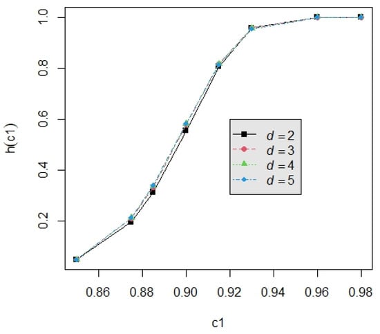
Figure 5. The power curve for n = 30; m = 5; p = 0.05; α = 0.05; and d = 2, 3, 4, and 5.

3.3. Example

For two production lines (d = 2), the data for the first production line consisted of the failure times (number of cycles) of n = 25 ball bearings in Caroni [19]. The data of 25 failure times U_1j, j = 1, …, 25, are listed as follows: 0.1788, 0.2892, 0.3300, 0.4152, 0.4212, 0.4560, 0.4848, 0.5184, 0.5196, 0.5412, 0.5556, 0.6780, 0.6780, 0.6780, 0.6864, 0.6864, 0.6888, 0.8412, 0.9312, 0.9864, 1.0512, 1.0584, 1.2792, 1.2804, and 1.7340. The p-value of the G test based on the Gini statistic (see Gail and Gastwirth [20]) is a function of the values of δ₁. The Gini statistic is obtained using $G_n=\frac{{\sum }_{j=1}^{n-1}j\left(n-j\right)\left(Y_{1(j+1)}-Y_{1\left(j\right)}\right)}{\left(n-1\right){\sum }_{j=1}^n\left(n-j+1\right)\left(Y_{1\left(j\right)}-Y_{1(j-1)}\right)},$ where $Y_{1\left(j\right)}=U_{1j}^{{\delta }_1}$, j = 1, …, 25. From Figure 6, we can see that the maximum p-value of 0.9882 occurred when the value of δ₁ = 2.58. Therefore, the value of δ₁ was determined to be δ₁ = 2.58.

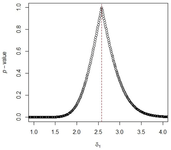
Figure 6. The p-values vs. the values of δ₁.

The large p-value indicated that the data fit the Weibull distribution well. For the failure times for production line 2, the simulated data of size n = 25 following a Weibull distribution with two parameters ${\delta }_2=$ 2 and ${\lambda }_2=$ 0.4 were generated as follows: 0.1416, 0.1823, 0.2083, 0.2151, 0.2337, 0.2435, 0.2536, 0.2742, 0.3082, 0.3109, 0.3148, 0.3160, 0.3409, 0.3483, 0.3725, 0.3837, 0.3987, 0.4046, 0.4057, 0.4342, 0.4511, 0.4658, 0.5038, 0.5322, and 0.6783.

Suppose that we wanted to test $H_0:C_T\le 0.85$. We created the progressive type I interval censored sample for the failure times of products from two production lines. Let the termination time T = 0.5 with a number of inspections m = 5, the equal length of inspection interval t = 0.1 (thousand cycles), and the pre-specified removal percentages of the remaining survival units given by (p₁, p₂, p₃, p₄, p₅) = (0.05, 0.05, 0.05, 0.05, 1.00).

The testing procedure was implemented as follows:

• Step 1: Given the known lower specification L₁ = L₂ = L = 0.01, we observed the progressive type I interval censored sample (X₁₁, X₁₂, X₁₃, X₁₄, X₁₅) = (0, 1, 1, 0, 3) and (X₂₁, X₂₂, X₂₃, X₂₄, X₂₅) = (0, 2, 6, 7, 2) for each production line at the pre-set times (t₁, …, t₅) = (0.1, 0.2, 0.3, 0.4, 0.5) with censoring schemes of (R₁₁, R₁₂, R₁₃, R₁₄, R₁₅) = (2, 2, 1, 1, 14) and (R₂₁, R₂₂, R₂₃, R₂₄, R₂₅) = (2, 2, 1, 1, 2).
• Step 2: Under the required level $c_0$ = 0.85 to achieve a pre-assigned conforming rate $P_r$ = 0.8607, we could determine the required target level $c_0^{*}=\frac{c_0+d-1}{d}=\frac{0.85+2-1}{2}$ = 0.9250 for each production line. Then, the testing hypothesis $H_0:C_{L_i}\le c_0^{*} \mathrm{for}\mathrm{some}i$ vs. $H_a:C_{L_i}>c_0^{*},i=1, 2$ was constructed.
• Step 3: We obtained the maximum likelihood estimators ${\widehat{k}}_1=$ 1.6973 and ${\widehat{k}}_2=$ 6.6993 for two production lines. We computed the values of the test statistics ${\widehat{C}}_{L_1}=1-1.6973\times 0.01=0.9830$ and ${\widehat{C}}_{L_2}=1-6.6993\times 0.01=0.9330$.
• Step 4: For the level of significance $\alpha$ = 0.1, we obtained ${\alpha }^{\prime }={0.1}^{\frac{1}{2}}=0.3162$ and $k_{10}=k_{20}=k_0=\frac{1-0.925}{0.01}=7.5$. Then, we calculated the critical values $C_{L_1}^0=1-\left(Z_{1-{\alpha }^{\prime }}\sqrt{I_1^{-1}\left(k_{10}\right)}+k_{10}\right)=0.9224$ and $C_{L_2}^0=1-\left(Z_{1-{\alpha }^{\prime }}\sqrt{I_2^{-1}\left(k_{20}\right)}+k_{20}\right)L=0.9238$ for the two production lines.
• Step 5: Since ${\widehat{C}}_{L_1}>C_{L_1}^0$ and ${\widehat{C}}_{L_2}>C_{L_2}^0,$ we could infer that both individual lifetime performance indices reached the desired target values so that the overall lifetime performance index reached the required level.

4. Conclusions

In various manufacturing domains, the analysis of lifetime performance indices is an important issue, especially when the lifespan of a product follows a Weibull distribution based on the progressive type I interval censored samples. Extending from the single production line to multiple production lines, we introduced an overall lifetime performance index applicable to these diverse production lines. Our investigation explored the interrelation between this overall lifetime performance index and the individual lifetime performance indices. We delved into the derivation of the maximum likelihood estimator and asymptotic distribution for both individual and overall lifetime performance indices based on the progressive type I interval censored samples. To assess whether the overall lifetime performance index achieved the targeted level, we developed a computational algorithm to conduct the proposed hypothesis testing procedure for a given level of significance. This involved testing each lifetime performance index using the maximum likelihood estimator as the test statistic. We scrutinized the impact of various configurations of the sample size n, the number of inspection intervals m, the removal probability p, the level of significance α, and particularly the number of production lines d on the test power through graphical representation Figure 1, Figure 2, Figure 3, Figure 4 and Figure 5. All findings are summarized in Section 3.2. We found that the test power was an increasing function of n, m, p, α, and d when the other parameters were fixed. To illustrate the practical application of our proposed testing algorithm for the overall lifetime performance index, we presented a numerical example with two production lines in Section 3.3.

References

- Montgomery, D.C. Introduction to Statistical Quality Control; John Wiley and Sons Inc.: New York, NY, USA, 1985. [Google Scholar]
- Anderson, D.R.; Sweeney, D.J.; Williams, T.A. Statistics for Business and Economics; West Publishing Company: Saint Paul, MN, USA, 1990. [Google Scholar]
- Meyer, P.L. Introductory Probability and Statistical Applications; Addison-Wesley: Reading, MA, USA, 1965. [Google Scholar]
- Epstein, B.; Sobel, M. Life-testing. J. Am. Stat. Assoc. 1953, 48, 486–502. [Google Scholar] [CrossRef]
- Tong, L.I.; Chen, K.S.; Chen, H.T. Statistical testing for assessing the performance of lifetime index of electronic components with exponential distribution. Int. J. Qual. Reliab. Manag. 2002, 19, 812–824. [Google Scholar] [CrossRef]
- Aggarwala, R. Progressive interval censoring: Some mathematical results with applications to inference. Commun. Stat. Theory Methods 2001, 30, 1921–1935. [Google Scholar] [CrossRef]
- Balakrishnan, N.; Aggarwala, R. Progressive Censoring: Theory, Methods and Applications; Birkhäuser: Boston, MA, USA, 2000. [Google Scholar]
- Hong, C.W.; Lee, W.C.; Wu, J.W. Computational Procedure of Performance Assessment of Lifetime Index of Products for the Weibull Distribution with the Progressive First-Failure-Censored Sampling Plan. J. Appl. Math. 2012, 2012, 717184. [Google Scholar] [CrossRef]
- Wu, J.W.; Lee, W.C.; Lin, L.S.; Hong, M.L. Bayesian test of lifetime performance index for exponential products based on the progressively type II right censored sample. J. Quant. Manag. 2011, 8, 57–77. [Google Scholar]
- Sanjel, D.; Balakrishnan, N. A Laguerre polynomial approximation for a goodness-of-fit test for exponential distribution based on progressively censored data. J. Stat. Comput. Simul. 2008, 78, 503–513. [Google Scholar] [CrossRef]
- Lee, W.C.; Wu, J.W.; Hong, C.W. Assessing the lifetime performance index of products with the exponential distribution under progressively type II right censored samples. J. Comput. Appl. Math. 2009, 231, 648–656. [Google Scholar] [CrossRef]
- Lee, H.M.; Wu, J.W.; Lei, C.L. Assessing the Lifetime Performance Index of Exponential Products with Step-Stress Accelerated Life-Testing Data. IEEE Trans. Reliab. 2013, 62, 296–304. [Google Scholar] [CrossRef]
- Wu, S.F.; Lin, M.J. Computational testing algorithmic procedure of assessment for lifetime performance index of products with weibull distribution under progressive type I interval censoring. J. Comput. Appl. Math. 2017, 311, 364–374. [Google Scholar] [CrossRef]
- Wu, S.F.; Wu, Y.C.; Wu, C.H.; Chang, W.T. Experimental design for the lifetime performance Index of Weibull products based on the progressive type I interval censored sample. Symmetry 2021, 13, 1691. [Google Scholar] [CrossRef]
- Wu, S.F.; Song, M.Z. The experimental design for the progressive type I interval censoring on the lifetime performance index of Chen lifetime distribution. Mathematics 2023, 11, 1554. [Google Scholar] [CrossRef]
- Wang, S.; Chen, W.; Chen, M.; Zhou, Y. Maximum likelihood estimation of the parameters of the inverse Gaussian distribution using maximum rank set sampling with unequal samples. Math. Popul. Stud. 2023, 30, 1–21. [Google Scholar] [CrossRef]
- Phaphan, W.; Simmachan, T.; Abdullahi, I. Maximum likelihood estimation of the weighted mixture generalized gamma distribution. Math. Stat. 2023, 11, 516–527. [Google Scholar] [CrossRef]
- Casella, G.; Berger, R.L. Statistical Inference, 2nd ed.; Duxbury Press: Pacific Grove, CA, USA, 2002. [Google Scholar]
- Caroni, C. The correct ”ball bearings” data. Lifetime Data Anal. 2002, 8, 395–399. [Google Scholar] [CrossRef] [PubMed]
- Gail, M.H.; Gastwirth, J.L. A scale-free goodness of fit test for the exponential distribution based on the Gini Statistic. J. R. Stat. Soc. B 1978, 40, 350–357. [Google Scholar] [CrossRef]
Disclaimer/Publisher’s Note: The statements, opinions and data contained in all publications are solely those of the individual author(s) and contributor(s) and not of MDPI and/or the editor(s). MDPI and/or the editor(s) disclaim responsibility for any injury to people or property resulting from any ideas, methods, instructions or products referred to in the content. |
© 2024 by the authors. Licensee MDPI, Basel, Switzerland. This article is an open access article distributed under the terms and conditions of the Creative Commons Attribution (CC BY) license (https://creativecommons.org/licenses/by/4.0/).