The Solution of the Extended 16th Hilbert Problem for Some Classes of Piecewise Differential Systems

Abstract

The limit cycles have a main role in understanding the dynamics of planar differential systems, but their study is generally challenging. In the last few years, there has been a growing interest in researching the limit cycles of certain classes of piecewise differential systems due to their wide uses in modeling many natural phenomena. In this paper, we provide the upper bounds for the maximum number of crossing limit cycles of certain classes of discontinuous piecewise differential systems (simply PDS) separated by a straight line and consequently formed by two differential systems. A linear plus cubic polynomial forms six families of Hamiltonian nilpotent centers. First, we study the crossing limit cycles of the PDS formed by a linear center and one arbitrary of the six Hamiltonian nilpotent centers. These six classes of PDS have at most one crossing limit cycle, and there are systems in each class with precisely one limit cycle. Second, we study the crossing limit cycles of the PDS formed by two of the six Hamiltonian nilpotent centers. There are systems in each of these 21 classes of PDS that have exactly four crossing limit cycles.

1. Introduction and Statement of the Main Results

In 1900, David Hilbert [1] shared a list of twenty-three problems at the International Congress of Mathematicians in Paris. From this list of problems, the sixteenth Hilbert problem is one of the remaining unsolved problems, together with the Riemann conjecture. The sixteenth Hilbert problem asks for the maximum number of limit cycles of a class of planar polynomial differential systems with a given degree. Recall that an isolated periodic orbit inside a planar differential system’s set of all periodic orbits is known as a limit cycle. In the qualitative study, one of the main problems of planar differential systems is determining the existence and the maximum number of limit cycles, see [2,3]. This importance comes from the main role of limit cycles for understanding and explaining the behavior of a given differential system, such as the limit cycle of the Belousov Zhavotinskii model [4] or the one of the Van der Pol equations [5,6], etc.

This work focuses on a class of planar PDS with two pieces, where the separation curve is the straight line $x=0$. Then, following the Filippov [7] conventions for defining this class of systems on the discontinuity line $x=0$, these PDS can be written as follows

$$\begin{array}{c}\hfill \left\{\begin{array}{c}{(\dot{x},\dot{y})}^T={(f^r(x,y),g^r(x,y))}^T,ifx\in R^r;\\ {(\dot{x},\dot{y})}^T={(f^l(x,y),g^l(x,y))}^T,ifx\in R^l,\end{array}\right.\end{array}$$

(1)

such that $R^r=\left\{(x,y)|x\ge 0\right\}$, and $R^l=\left\{(x,y)|x\le 0\right\}$. These systems can exhibit either crossing limit cycles or sliding limit cycles. Here, we are only interested in the crossing ones, which are isolated periodic orbits having exactly two crossing points, i.e., the limit cycle intersects the straight line $x=0$ in two points $(0,y_i)$ with $i=1,2$ such that $f^r(0,y_i)f^l(0,y_i)\ge 0$ for $i=0,1$. Rather than saying “crossing limit cycle”, we will refer to it as “limit cycle”.

In the 1920s, Andronov and coworkers [8] started the serious study of PDS. Nowadays, these systems are a more important research subject for many scientists. This is due to the relevant applications of PDS to model many problems in mechanics, economics, control theory, medicine, biology, etc., as we can see in [9,10,11].

In recent years, several authors have paid more attention to the simplest class of PDS, the ones separated by a straight line and consequently formed by two pieces, having a linear differential system in each piece; see [12,13,14], as well as the references cited in these works. Since all the results in the published papers provide only examples of planar PDS with at most three limit cycles, it still needs to be discovered whether three is the maximum number of limit cycles for this class of systems. Recently, Benterki and Llibre [15] studied the extension of the 16th Hilbert problem to PDS having isochronous centers of degree one or three. Then, from here, we build the main objective of this paper, where we study the problem of the existence and the maximum number of limit cycles for two different families of PDS separated by the straight line $x=0$.

We denote by ${\mathcal{F}}_1$ the family of PDS separated the straight line $x=0$ on two pieces. In one piece, there is an arbitrary linear differential center. In the other one, there is a Hamiltonian nilpotent center formed by a linear plus cubic homogeneous polynomial after an arbitrary affine change in the variables.

We denote by ${\mathcal{F}}_2$ the family of PDS separated by the straight line $x=0$ on two pieces; in each piece, there is an arbitrary Hamiltonian nilpotent center formed by a linear plus cubic homogeneous polynomials after an arbitrary affine change in the variables.

We shall use the following lemma for the first family of planar differential systems, which provides the normal form of any arbitrary linear differential center.

Lemma 1.

By conducting a linear change in the variables and a rescaling of the independent variable, any linear center in ${\mathbb{R}}^2$ can be expressed as follows

$$\begin{array}{c}\hfill \dot{x}=C-Bx-{\displaystyle \frac{\left(k^2+4B^2\right)}{4A}}y,\dot{y}=D+Ax+By,\end{array}$$

(2)

with $A,k>0$, and its first integral is

$$\begin{array}{c}\hfill H(x,y)=8A(Dx-Cy)+4{(Ax+By)}^2+k^2{y}^2.\end{array}$$

(3)

For a short proof of Lemma 1, see Section 3.

Our results use the previous results of [16] as follows.

Theorem 1.

After doing a linear change of variables and rescaling of the independent variable, every Hamiltonian planar polynomial differential system with linear plus cubic homogeneous terms has a nilpotent center at the origin that can be expressed as one of the following six classes:

$\left({\mathcal{C}}_1\right)$

$\dot{x}=\alpha x+\beta y,\dot{y}={\displaystyle \frac{-{\alpha }^2}{\beta }}x-\alpha y+x^3$, with $\beta <0$.

$\left({\mathcal{C}}_2\right)$

$\dot{x}=\alpha x+\beta y-x^3,\dot{y}={\displaystyle \frac{-{\alpha }^2}{\beta }}x-\alpha y+3x^{2}y$, with $\beta \ne 0$ and $\alpha >0$.

$\left({\mathcal{C}}_3\right)$

$\dot{x}=\alpha x+\beta y-3x^{2}y+y^3,\dot{y}=\eta x-\alpha y+3x{y}^2$, with either $\beta =\alpha =0$ and $\gamma <0$, or $\gamma =0$, $\alpha \beta \ne 0$, and ($6\beta <{\alpha }^2/\beta )$ or simply we can take $\alpha =1$).

$\left({\mathcal{C}}_4\right)$

$\dot{x}=\alpha x+\beta y-3x^{2}y-y^3,\dot{y}=\eta x-\alpha y+3x{y}^2$, with either $\beta =\alpha =0$ and $\gamma >0$, or $\gamma =0$, $\beta <0$, and ($\alpha \ne 0$, or we can simply take $\alpha =1$).

$\left({\mathcal{C}}_5\right)$

$\dot{x}=\alpha x+\beta y-3\delta x^{2}y+y^3,\dot{y}=\eta x-\alpha y+x^3+3\delta x{y}^2$, with either $\beta =\alpha =0$ and $\gamma <0$, or $\gamma =0$, $\beta \ne 0$, and ($({\alpha }^4-{\beta }^4-6\delta {\alpha }^2{\beta }^2)/\beta >0$, or we can simply take $\alpha =1$).

$\left({\mathcal{C}}_6\right)$

$\dot{x}=\alpha x+\beta y-3\delta x^{2}y-y^3,\dot{y}=\eta x-\alpha y+x^3+3\delta x{y}^2$, with either $\gamma >0$ and $\beta =\alpha =0$, or $\gamma =0$, $\beta \ne 0$, and ($({\alpha }^4+{\beta }^4+6\delta {\alpha }^2{\beta }^2)/\beta <0$, or we can simply take $\alpha =1$).

Here, $\eta =\left({\displaystyle \frac{\gamma (\beta +\gamma )-{\alpha }^2}{\beta +\gamma }}\right)$, and $\alpha ,\beta ,\gamma ,\delta \in \mathbb{R}$.

Our main results are the following seven theorems.

Theorem 2.

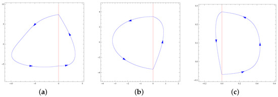
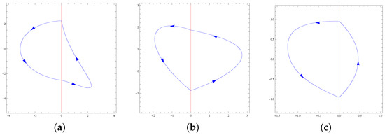
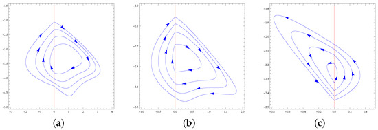
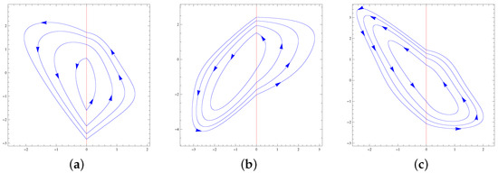
The maximum number of limit cycles of the family ${\mathcal{F}}_1$ is one. This maximum is reached in all the classes; see Figure 1 and Figure 2.

Figure 1. (a) The unique limit cycle of PDS (12) and (13), (b) the unique limit cycle of PDS (14) and (15), and (c) the unique limit cycle of PDS (16) and (17).

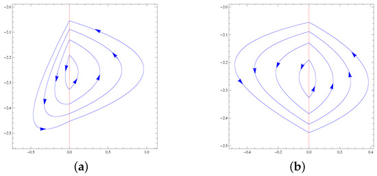
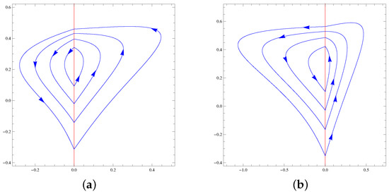
Figure 2. (a) The unique limit cycle of PDS (18) and (19), (b) the unique limit cycle of PDS (20) and (21), and (c) the unique limit cycle of PDS (22) and (23).

For the proof of Theorem 2, see Section 3.

Theorem 3.

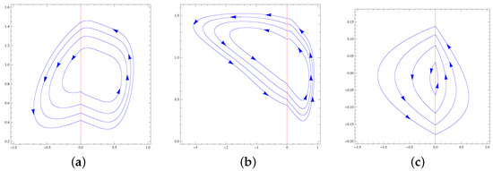
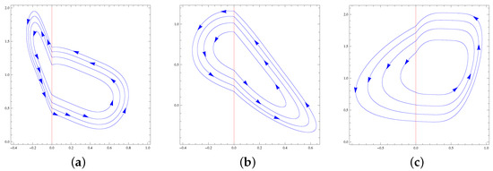
The maximum number of limit cycles of systems of the family ${\mathcal{F}}_2$ formed by a Hamiltonian nilpotent center $\left({\mathcal{C}}_1\right)$ in one region and by one of the Hamiltonian nilpotent centers $\left({\mathcal{C}}_i\right)$ with $i=1,\dots ,6$ in the other region is four. For every class, this maximum is achieved; see Figure 3 and Figure 4.

Figure 3. (a) The four limit cycles of PDS (26) and (27), (b) the four limit cycles of PDS (28) and (29), and (c) the four limit cycles of PDS (30) and (31).

Figure 4. (a) The four limit cycles of PDS (32) and (33), (b) the four limit cycles of PDS (34) and (35), and (c) the four limit cycles of the PDS (36) and (37).

Theorem 4.

The maximum number of limit cycles of systems of the family ${\mathcal{F}}_2$ formed by a Hamiltonian nilpotent center $\left({\mathcal{C}}_2\right)$ in one region and by one of the Hamiltonian nilpotent centers $\left({\mathcal{C}}_i\right)$ with $i=2,\dots ,6$ in the other region is four. For every class, this maximum is achieved; see Figure 5 and Figure 6.

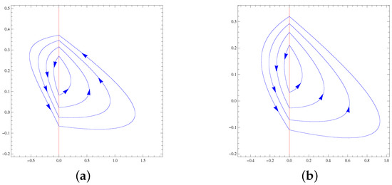
Figure 5. (a) The four limit cycles of PDS (38) and (39), (b) he four limit cycles of PDS (40) and (41), and (c) the four limit cycles of PDS (42) and (43).

Figure 6. (a) The four limit cycles of PDS (44) and (45), and (b) the four limit cycles of PDS (46) and (47).

Theorem 5.

The maximum number of limit cycles of systems of the family ${\mathcal{F}}_2$ formed by a Hamiltonian nilpotent center $\left({\mathcal{C}}_3\right)$ in one region and by one of the Hamiltonian nilpotent centers $\left({\mathcal{C}}_i\right)$ with $i=3,\dots ,6$ in the other region is four. For every class, this maximum is achieved; see Figure 7 and Figure 8.

Figure 7. (a) The four limit cycles of PDS (48) and (49), and (b) the four limit cycles of PDS (50) and (51).

Figure 8. (a) The four limit cycles of PDS (52) and (53), and (b) the four limit cycles of PDS (54) and (55).

Theorem 6.

The maximum number of limit cycles of systems of the family ${\mathcal{F}}_2$ formed by a Hamiltonian nilpotent center $\left({\mathcal{C}}_4\right)$ in one region and by one of the Hamiltonian nilpotent centers $\left({\mathcal{C}}_i\right)$ with $i=4,\dots ,6$ in the other region is four. This maximum is achieved for all the classes, see Figure 9.

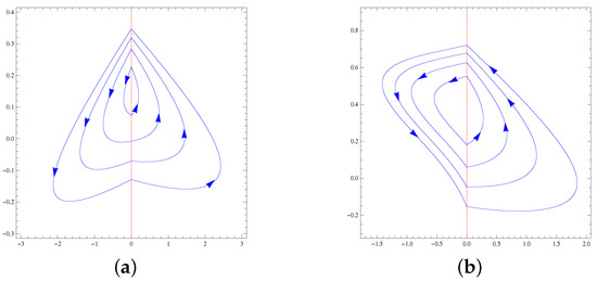
Figure 9. (a) The four limit cycles of PDS (56) and (57), (b) the four limit cycles of PDS (58) and (59), and (c) the four limit cycles of PDS (60) and (61).

Theorem 7.

The maximum number of limit cycles of systems of the family ${\mathcal{F}}_2$ formed by a Hamiltonian nilpotent center $\left({\mathcal{C}}_5\right)$ in one region and by one of the Hamiltonian nilpotent centers $\left({\mathcal{C}}_5\right)$ or $\left({\mathcal{C}}_6\right)$ in the other region is four. For any class, this maximum is achieved; see Figure 10.

Figure 10. (a) The four limit cycles of PDS (62) and (63), and (b) the four limit cycles of PDS (64) and (65).

Theorem 8.

The maximum number of limit cycles of systems of the family ${\mathcal{F}}_2$ formed by a Hamiltonian nilpotent center $\left({\mathcal{C}}_6\right)$ in each region is four. This maximum is achieved; see Figure 11.

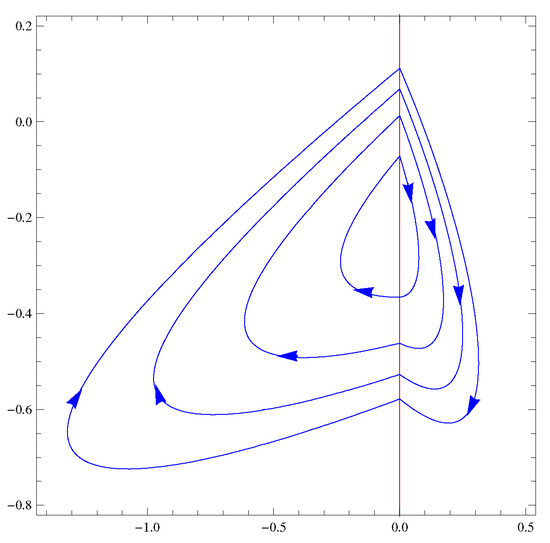
Figure 11. The four limit cycles of PDS (66) and (67).

For the proof of Theorems 3–8 see Section 5.

2. The General Hamiltonian Nilpotent Centers $\left({\mathcal{C}}_{\mathbf{1}}\right)$, $\left({\mathcal{C}}_{\mathbf{2}}\right)$, $\left({\mathcal{C}}_{\mathbf{3}}\right)$, $\left({\mathcal{C}}_{\mathbf{4}}\right)$, $\left({\mathcal{C}}_{\mathbf{5}}\right)$, and $\left({\mathcal{C}}_{\mathbf{6}}\right)$ after an Affine Change of Variables

This section deals with a general affine change in the variables in the expression of the Hamiltonian planar polynomial differential systems with a linear plus cubic homogeneous term having a nilpotent center $\left({\mathcal{C}}_1\right)$, $\left({\mathcal{C}}_2\right)$, $\left({\mathcal{C}}_3\right)$, $\left({\mathcal{C}}_4\right)$, $\left({\mathcal{C}}_5\right)$, or $\left({\mathcal{C}}_6\right)$ and of their the first integrals. By applying the change in the variables

$$(x,y)=(c_1+a_{1}x+b_{1}y,c_2+a_{2}x+b_{2}y),$$

with $a_2{b}_1-a_1{b}_2\ne 0$, the differential nilpotent center $\left({\mathcal{C}}_1\right)$

$$\begin{array}{cc}\hfill \dot{x}=& {\displaystyle \frac{1}{\beta (a_2{b}_1-a_1{b}_2)}}(-{\alpha }^2{b}_1(c_1+a_{1}x+b_{1}y)+\beta (3b_1^3{y}^2(a_{1}x+c_1)+3b_1^{2}y(a_{1}x+\hfill \\ \hfill & c_1{)}^2+b_1{(a_{1}x+c_1)}^3+b_1^4{y}^3-\beta b_2(a_{2}x+c_2+b_{2}y))-\alpha \beta \hfill \\ \hfill & (b_2(a_{1}x+c_1)+b_1(c_2{a}_{2}x+2b_{2}y))),\hfill \\ \hfill \dot{y}=& {\displaystyle \frac{1}{\beta (a_2{b}_1-a_1{b}_2)}}({\alpha }^2{a}_1(c_1+a_{1}x+b_{1}y)+\beta (-a_1^4{x}^3-3a_1^3{x}^2(b_{1}y+c_1)-3a_1^{2}x(b_1\hfill \\ \hfill & y+c_1{)}^2-a_1{(b_{1}y+c_1)}^3+a_2\beta (a_{2}x+c_2+b_{2}y))+\alpha \beta (a_1(c_2\hfill \\ \hfill & +2a_{2}x+b_{2}y)+a_2{b}_{1}y+a_2{c}_1)),\hfill \end{array}$$

(4)

with the first integral

$$\begin{array}{ccc}\hfill H_1(x,y)& =& {\displaystyle \frac{{\alpha }^2}{2\beta }}{(c_1+a_{1}x+b_{1}y)}^2+\alpha (c_1+a_{1}x+b_{1}y)(a_{2}x+c_2+b_{2}y)-{\displaystyle \frac{1}{4}}(a_{1}x\hfill \\ & & +b_{1}y+c_1{)}^4+{\displaystyle \frac{1}{2}}\beta {(a_{2}x+c_2+b_{2}y)}^2.\hfill \end{array}$$

The differential nilpotent center $\left({\mathcal{C}}_2\right)$ becomes

$$\begin{array}{cc}\hfill \dot{x}=& {\displaystyle \frac{1}{\beta (a_2{b}_1-a_1{b}_2)}}(\beta b_1^3{y}^2(3c_2+3a_{2}x+4b_{2}y)-\beta b_2(\alpha a_{1}x-a_1^3{x}^3-3a_1{c}_1^{2}x-\hfill \\ \hfill & c_1^3+c_1(\alpha -3a_1^2{x}^2)+\beta (a_{2}x+c_2+b_{2}y))+b_1^{2}y(3\beta (a_{1}x+\hfill \\ \hfill & c_1)(2c_2+2a_{2}x+3b_{2}y)-{\alpha }^2)+b_1\left(3\beta c_1^2\right(c_2+a_{2}x+2b_2\hfill \\ \hfill & y)-{\alpha }^2{a}_{1}x+3a_1^2\beta x^2(c_2+a_{2}x+2b_{2}y)-ab(c_2+a_{2}x+2\hfill \\ \hfill & b_{2}y)+c_1{a}_1\beta x(c_2+a_{2}x+2b_{2}y)-{\alpha }^2\left)\right),\hfill \\ \hfill \dot{y}=& {\displaystyle \frac{1}{\beta (a_2{b}_1-a_1{b}_2)}}(a_2\beta -a_1^3\beta x^2(4a_{2}x+3(c_2+b_{2}y))(\alpha b_{1}y-b_1^3{y}^3-3b_1{c}_1^{2}y\hfill \\ \hfill & -c_1^3+c_1(\alpha -3b_1^2{y}^2)+\beta (a_{2}x+c_2+b_{2}y))-a_1^{2}x\left(3\beta \right(b_{1}y\hfill \\ \hfill & +c_1)(3a_{2}x+2(c_2+b_{2}y))-{\alpha }^2)+a_1(-3\beta c_1^2(c_2+2a_{2}x\hfill \\ \hfill & +b_{2}y)+{\alpha }^2{b}_{1}y+c_1({\alpha }^2-6\beta b_{1}y(c_2+2a_{2}x+b_{2}y))+\alpha \beta \hfill \\ \hfill & (c_2+2a_{2}x+b_{2}y)-3\beta b_1^2{y}^2(c_2+2a_{2}x+b_{2}y)\left)\right),\hfill \end{array}$$

(5)

and its first integral is

$$\begin{array}{ccc}\hfill H_2(x,y)& =& {\displaystyle \frac{{\alpha }^2}{2\beta }}{(c_1+a_{1}x+b_{1}y)}^2+\alpha (c_1+a_{1}x+b_{1}y)(a_{2}x+c_2+b_{2}y)+{\displaystyle \frac{1}{2}}\beta \hfill \\ & & {(a_{2}x+c_2+b_{2}y)}^2-{(c_1+a_{1}x+b_{1}y)}^3(a_{2}x+c_2+b_{2}y).\hfill \end{array}$$

The differential center $\left({\mathcal{C}}_3\right)$ becomes

$$\begin{array}{cc}\hfill \dot{x}=& {\displaystyle \frac{-1}{(\beta +\gamma )(a_2{b}_1-a_1{b}_2)}}({\alpha }^2{b}_1(c_1+a_{1}x+b_{1}y)+\alpha (\beta +\gamma )(b_2(a_{1}x+c_1)+b_1\hfill \\ \hfill & (c_2+a_{2}x+2b_{2}y))+(\beta +\gamma )(b_2(a_{2}x+c_2+b_{2}y)\hfill \\ \hfill & (-3a_1^2{x}^2-6a_1{c}_{1}x+\beta -3c_1^2+{(c_2+a_{2}x+b_{2}y)}^2)\hfill \\ \hfill & -b_1(a_{1}x+c_1)(\gamma +3(a_{2}x+c_2+b_{2}y)(c_2+a_{2}x+3\hfill \\ \hfill & b_{2}y))-b_1^{2}y(\gamma +3(c_2+a_{2}x+b_{2}y)(c_2+a_{2}x+2b_2\hfill \\ \hfill & y)))),\hfill \\ \hfill \dot{y}=& {\displaystyle \frac{1}{(\beta +\gamma )(a_2{b}_1-a_1{b}_2)}}({\alpha }^2{a}_1(c_1+a_{1}x+b_{1}y)+\alpha (\beta +\gamma )(a_1(c_2+2a_{2}x+b_{2}y)\hfill \\ \hfill & +a_2{b}_{1}y+a_2{c}_1)-(\beta +\gamma )(-a_2(a_{2}x+c_2+b_{2}y)(\beta -3\hfill \\ \hfill & b_1^2{y}^2-6b_1{c}_{1}y-3c_1^2+{(c_2+a_{2}x+b_2+y)}^2)a_1^{2}x(\gamma +3\hfill \\ \hfill & (a_{2}x+c_2+b_{2}y)(c_2+2a_{2}x+b_{2}y))(b_{1}y+a_1+c_1)(\gamma \hfill \\ \hfill & +3(c_2+a_{2}x+b_{2}y)(c_2+3a_{2}x+b_{2}y)))),\hfill \end{array}$$

(6)

and its first integral is

$$\begin{array}{ccc}\hfill H_3(x,y)& =& {\displaystyle \frac{1}{2}}\left({\displaystyle \frac{{\alpha }^2}{\beta +\gamma }}-\gamma \right){(c_1+a_{1}x+b_{1}y)}^2+\alpha (c_1+a_{1}x+b_{1}y)(c_2+a_{2}x\hfill \\ & & +b_{2}y)+{\displaystyle \frac{1}{2}}\beta {(a_{2}x+c_2+b_{2}y)}^2-{\displaystyle \frac{3}{2}}{(c_1+a_{1}x+b_{1}y)}^2(c_2+a_{2}x\hfill \\ & & +b_2{y)}^2+{\displaystyle \frac{1}{4}}{(a_{2}x+c_2+b_{2}y)}^4.\hfill \end{array}$$

The differential nilpotent center $\left({\mathcal{C}}_4\right)$ becomes

$$\begin{array}{cc}\hfill \dot{x}=& -{\displaystyle \frac{1}{(\beta +\gamma )(a_2{b}_1-a_1{b}_2)}}({\alpha }^2{b}_1(c_1+a_{1}x+b_{1}y)+\alpha (\beta +\gamma )(b_2(a_{1}x+c_1)+b_1(c_2\hfill \\ \hfill & +a_{2}x+2b_{2}y\left)\right)+(-b_2(a_{2}x+c_2+b_{2}y)(3a_1^2{x}^2+6a_1\hfill \\ \hfill & c_{1}x-\beta +3c_1^2+{(a_{2}x+c_2+b_{2}y)}^2)+b_1^{2}y(\gamma +3(c_2+\hfill \\ \hfill & a_{2}x+b_{2}y)(c_2+a_{2}x+2b_{2}y))-b_1(a_{1}x+c_1)(\gamma +3\hfill \\ \hfill & (a_{2}x+c_2+b_{2}y)(c_2+a_{2}x+3b_{2}y)\left)\right),\hfill \\ \hfill \dot{y}=& {\displaystyle \frac{1}{(\beta +\gamma )(a_2{b}_1-a_1{b}_2)}}({\alpha }^2{a}_1(c_1+a_{1}x+b_{1}y)+\alpha (\beta +\gamma )(a_1(c_2+2a_{2}x+b_{2}y)\hfill \\ \hfill & +a_2{b}_{1}y+a_2{c}_1)-(\beta +\gamma )(a_2(a_{2}x+c_2+b_{2}y)(-\beta +3\hfill \\ \hfill & b_1^2{y}^2+6b_1{c}_{1}y+3c_1^2+{(c_2+a_{2}x+b_{2}y)}^2)+a_1^{2}x(\gamma +3\hfill \\ \hfill & (a_{2}x+c_2+b_{2}y)(c_2+2a_{2}x+b_{2}y))+a_1(b_{1}y+c_1)\hfill \\ \hfill & (\gamma +3)(a_{2}x+c_2+b_{2}y)(c_2+3\hfill \\ \hfill & a_{2}x+b_{2}y\left)\right)),\hfill \end{array}$$

(7)

with the first integral

$$\begin{array}{ccc}\hfill H_4(x,y)& =& -{\displaystyle \frac{1}{2}}\left(\gamma -{\displaystyle \frac{{\alpha }^2}{\beta +\gamma }}\right){(c_1+a_{1}x+b_{1}y)}^2+\alpha (c_1+a_{1}x+b_{1}y)(c_2+a_{2}x\hfill \\ & & +b_{2}y)+{\displaystyle \frac{1}{2}}\beta {(a_{2}x+c_2+b_{2}y)}^2-{\displaystyle \frac{3}{2}}{(c_1+a_{1}x+b_{1}y)}^2(c_2+a_{2}x+\hfill \\ & & b_2{y)}^2-{\displaystyle \frac{1}{4}}{(a_{2}x+c_2+b_{2}y)}^4.\hfill \end{array}$$

The differential nilpotent center $\left({\mathcal{C}}_5\right)$ becomes

$$\begin{array}{cc}\hfill \dot{x}=& -{\displaystyle \frac{1}{(\beta +\gamma )(a_2{b}_1-a_1{b}_2)}}({\alpha }^2{b}_1(c_1+a_{1}x+b_{1}y)+\alpha (\beta +\gamma )(b_2(a_{1}x+c_1)+b_1\hfill \\ \hfill & (c_2+a_{2}x+2b_{2}y))+(\beta +\gamma )(-3b_1^3{y}^2(a_{1}x+c_1)+\hfill \\ \hfill & b_2(a_{2}x+c_2+b_{2}y)(-3\delta {(a_{1}x+c_1)}^2+\beta +(c_2+a_2\hfill \\ \hfill & x+b_2{y)}^2)-b_1^4{y}^3-b_1(a_{1}x+c_1)({(a_{1}x+c_1)}^2+\gamma +\hfill \\ \hfill & 3\delta (c_2+a_{2}x+b_{2}y)(c_2+a_{2}x+3b_{2}y))-b_1^{2}y\left(3\right((a_1\hfill \\ \hfill & x+c_1{)}^2+\delta (c_2+a_{2}x+b_{2}y)(c_2+a_{2}x+2b_{2}y))\hfill \\ \hfill & +\gamma \left)\right)),\hfill \\ \hfill \dot{y}=& {\displaystyle \frac{1}{(\beta +\gamma )(a_2{b}_1-a_1{b}_2)}}({\alpha }^2{a}_1(c_1+a_{1}x+b_{1}y)+\alpha (\beta +\gamma )(a_1(c_2+2a_{2}x+b_{2}y)\hfill \\ \hfill & +a_2{b}_{1}y+a_2{c}_1)-(\beta +\gamma )(+3a_1^3{x}^2(b_{1}y+c_1)+a_2(c_2\hfill \\ \hfill & +a_{2}x+b_{2}y\left)\right(-b+3\delta {(b_{1}y+c_1)}^2-(c_2+a_{2}x+b_2\hfill \\ \hfill & {y)}^2)+a_1^4{x}^3+a_1(b_{1}y+c_1)({(b_{1}y+c_1)}^2+\gamma +3\delta (c_2\hfill \\ \hfill & +a_{2}x+b_{2}y)(c_2+3a_{2}x+b_{2}y))+a_1^{2}x\left(3\right({(b_{1}y+c_1)}^2\hfill \\ \hfill & +\delta (c_2+a_{2}x+b_{2}y)(c_2+2a_{2}x+b_{2}y))+\gamma )\left)\right),\hfill \end{array}$$

(8)

with the first integral

$$\begin{array}{ccc}\hfill H_5(x,y)& =& {\displaystyle \frac{1}{2}}\left({\displaystyle \frac{{\alpha }^2}{\beta +\gamma }}-\gamma \right){(c_1+a_{1}x+b_{1}y)}^2+\alpha (c_1+a_{1}x+b_{1}y)(a_{2}x+c_2+b_{2}y)\hfill \\ & & -{\displaystyle \frac{1}{4}}{(c_1+a_{1}x+b_{1}y)}^4-{\displaystyle \frac{3}{2}}\delta {(c_1+a_{1}x+b_{1}y)}^2{(a_{2}x+c_2+b_{2}y)}^2+{\displaystyle \frac{1}{2}}\beta \hfill \\ & & {(a_{2}x+c_2+b_{2}y)}^2+{\displaystyle \frac{1}{4}}{(a_{2}x+c_2+b_{2}y)}^4.\hfill \end{array}$$

Finally, the differential nilpotent center $\left({\mathcal{C}}_6\right)$ becomes

$$\begin{array}{cc}\hfill \dot{x}=& {\displaystyle \frac{-1}{(\beta +\gamma )(a_2{b}_1-a_1{b}_2)}}({\alpha }^2{b}_1(c_1+a_{1}x+b_{1}y)+\alpha (\beta +\gamma )(b_2(a_{1}x+c_1)+b_1(c_2\hfill \\ \hfill & +a_{2}x+2b_{2}y))+(\beta +\gamma )(-b_2{a}_{2}x+c_2+b_{2}y(3\delta (a_{1}x\hfill \\ \hfill & +c_1{)}^2-\beta +{(c_2+a_{2}x+b_{2}y)}^2-3b_1^3{y}^2(a_{1}x+c_1)-b_1^4\hfill \\ \hfill & y^3-b_1(a_{1}x+c_1)({(a_{1}x+c_1)}^2+\gamma +3\delta (a_{2}x+c_2+b_{2}y)\hfill \\ \hfill & (c_2+a_{2}x+b_{2}y))-b_1^{2}y(3({(a_{1}x+c_1)}^2+\delta (c_2+a_{2}x+\hfill \\ \hfill & b_{2}y)(c_2+a_{2}x+2b_{2}y))+\gamma ))),\hfill \\ \hfill \dot{y}=& {\displaystyle \frac{1}{(\beta +\gamma )(a_2{b}_1-a_1{b}_2)}}({\alpha }^2{a}_1(c_1+a_{1}x+b_{1}y)+\alpha (\beta +\gamma )(a_1(c_2+2a_{2}x+b_{2}y)\hfill \\ \hfill & +a_2{b}_{1}y+a_2{c}_1)-(\beta +\gamma )(3a_1^3{x}^2(b_{1}y+c_1)+a_2(c_2+\hfill \\ \hfill & a_{2}x+b_{2}y)(-\beta +3\delta {(b_{1}y+c_1)}^2+{(c_2+a_{2}x+b_{2}y)}^2)\hfill \\ \hfill & +a_1^4{x}^3+a_1(b_{1}y+c_1)({(b_{1}y+c_1)}^2+\gamma +3\delta (c_2+a_{2}x+\hfill \\ \hfill & b_{2}y)(c_2+3a_{2}x+b_{2}y))+a_1^{2}x(3({(b_{1}y+c_1)}^2+\delta (c_2+\hfill \\ \hfill & a_{2}x+b_{2}y)(c_2+2a_{2}x+b_{2}y))+\gamma ))),\hfill \end{array}$$

(9)

with the first integral

$$\begin{array}{ccc}\hfill H_6(x,y)& =& {\displaystyle \frac{1}{2}}\left({\displaystyle \frac{{\alpha }^2}{\beta +\gamma }}-\gamma \right){(c_1+a_{1}x+b_{1}y)}^2+\alpha (c_1+a_{1}x+b_{1}y)(a_{2}x+c_2+b_{2}y)\hfill \\ & & -{\displaystyle \frac{1}{4}}{(c_1+a_{1}x+b_{1}y)}^4-{\displaystyle \frac{3}{2}}\delta {(c_1+a_{1}x+b_{1}y)}^2{(a_{2}x+c_2+b_{2}y)}^2+{\displaystyle \frac{1}{2}}\beta \hfill \\ & & {(a_{2}x+c_2+b_{2}y)}^2-{\displaystyle \frac{1}{4}}{(a_{2}x+c_2+b_{2}y)}^4.\hfill \end{array}$$

3. Proof of Lemma 1 and Theorem 2

This section starts with the proof of Lemma 1.

Proof. 

A linear differential system in the plane has the form

$$\begin{array}{cc}\hfill \dot{x}=& C+ax+by,\dot{y}=D+Ax+By.\hfill \end{array}$$

(10)

We know that ${\displaystyle \frac{1}{2}}(a+B\pm \sqrt{{(a-B)}^2+4Ab})$ are the eigenvalues of system (10). Therefore, in order for this system to have a center, we must take

$$a=-B,{(a-B)}^2+4Ab=-k^2,\mathrm{with}k>0.$$

Then, $b={\displaystyle \frac{-(k^2+4B^2)}{4A}}$ and $A>0$. Under these conditions the linear system (10) becomes

$$\begin{array}{cc}\hfill \dot{x}=& C-Bx-{\displaystyle \frac{(k^2+4B^2)}{4A}}y,\dot{y}=D+Ax+By.\hfill \end{array}$$

The proof of Lemma 1 is complete.  □

Now, we have to prove Theorem 2 for the class of PDS separated by the line $x=0$ and formed by the pair of differential systems (2)-$\left(i\right)$, for $i\in \{4,\dots ,9\}$.

Proof. 

In the right region $R^r$, we consider the linear differential center (2), with its corresponding first integral $H(x,y)$ given by (3). In the left region $R^l$, we consider the Hamiltonian differential nilpotent center $\left(i\right)$, with its first integral $H_{i-3}(x,y)$. Now, if the PDS (2)-$\left(i\right)$ has a limit cycle, it must cross the separation line $x=0$ at pair of distinct points $p_1=(0,y_1)$ and $p_2(0,y_2)$, where $y_1<y_2$. Moreover, $p_1$ and $p_2$ must satisfy the following system

$$\begin{array}{cc}\hfill H\left(p_1\right)-H\left(p_2\right)=& (y_2-y_1)(2CA-B^2{y}_1-B^2{y}_2-k^2(y_2-y_1)),\hfill \\ \hfill =& (y_2-y_1)h(y_1,y_2),\hfill \\ \hfill H_{i-3}\left(p_1\right)-H_{i-3}\left(p_2\right)=& h_{i-3}(y_1,y_2),\hfill \end{array}$$

(11)

where the two polynomials $h(y_1,y_2)$ and $h_{i-3}(y_1,y_2)$, for all $i\in \{4,\dots ,9\}$, are of degrees one and three, respectively. Since $y_1<y_2$, solving $h(y_1,y_2)=0$, we obtain $y_2=g\left(y_1\right)$, which is a function of the variable $y_1$. After substituting the expression of $y_2$ in $h_{i-3}(y_1,y_2)=0$, we obtain a new quadratic equation with $y_1$ as the unknown variable. It is clear that there are at most two real solutions, $(y,f(y\left)\right)$ and $(Y,f(Y\left)\right)$, for this equation. Due to the symmetry $(y,f(y\left)\right)=\left(f\right(Y),Y)$, we know that these two solutions represent the same solution of (11). Then, for PDS (2)-$\left(i\right)$, both solutions offer the same limit cycle. It has been demonstrated that PDS (2)-$\left(i\right)$ has a maximum of one limit cycle.  □

4. Numerical Examples of Theorem 2

One limit cycle for the class formed by system (2) and (4). In what follows, we give a PDS of the class (2) and (4) with exactly one limit cycle. In $R^l$, we consider the nilpotent center

$$\begin{array}{cc}\hfill \dot{x}=& {\displaystyle \frac{1}{1500100}}\left(100\right(-x^3-30x^2(y-1)+x(13714-300(y-2)y)-1000(y-3)\hfill \\ \hfill & y^2)-1302001y+1050950),\hfill \\ \hfill \dot{y}=& {\displaystyle \frac{1}{150010}}(x^3+30x^2(y-1)+100x(3(y-2)y+1963)+20\left(y\right(50(y-3)y\hfill \\ \hfill & -6857)+6600)),\hfill \end{array}$$

(12)

of the form (4); this system has the first integral

$$\begin{array}{cc}\hfill H_1(x,y)=& -{\displaystyle \frac{1}{4}}{\left({\displaystyle \frac{x}{10}}-1+y\right)}^4-5{\left({\displaystyle \frac{x}{10}}-1+y\right)}^2-\left({\displaystyle \frac{y+50}{100}}-15x\right)({\displaystyle \frac{x}{10}}+y-1)\hfill \\ \hfill & -{\displaystyle \frac{1}{200000}}{(-1500x+y+50)}^2.\hfill \end{array}$$

In $R^r$, we consider the linear differential system

$$\begin{array}{c}\hfill \dot{x}=-{\displaystyle \frac{x}{10}}-{\displaystyle \frac{101y}{1000}}+{\displaystyle \frac{1}{10}},\dot{y}={\displaystyle \frac{x}{10}}+{\displaystyle \frac{y}{10}}+{\displaystyle \frac{1}{2}},\end{array}$$

(13)

which has

$$H(x,y)={\displaystyle \frac{1}{10000}}(200(x-1)y+100x(x+10)+101y^2),$$

as a first integral. Now, we focus on the solutions of system (11) with $i=4$ satisfying $y_1<y_2$. The unique solution of (11) is $(y_1,y_2)\approx (-5.45516,7.43536),$ and it provides the unique limit cycle of PDS (12) and (13) shown in Figure 1a.

One limit cycle for the class formed by system (2) and (5). Here, we take the nilpotent center (5) in the left region $R^l$

$$\begin{array}{cc}\hfill \dot{x}=& {\displaystyle \frac{1}{290000}}(91x^3+60x^2(455-31y)+300x(y(33y-950)+7722)-1000(y\hfill \\ \hfill & \left(4\right(y-30)y+981)+585\left)\right),\hfill \\ \hfill \dot{y}=& {\displaystyle \frac{1}{290000}}(12x^3+4035x^2+60(31x+2375)y^2-39(7x(x+200)+59400)y\hfill \\ \hfill & +1294510x-3300y^3+7844000,\hfill \end{array}$$

(14)

whixh has

$$\begin{array}{ccc}\hfill H_2(x,y)& =& {\displaystyle \frac{1}{10}}\left(-{\displaystyle \frac{x}{100}}+{\displaystyle \frac{y}{10}}-{\displaystyle \frac{3}{2}}\right)(-3x+y+5)-{\displaystyle \frac{1}{20}}{\left(-{\displaystyle \frac{x}{100}}+{\displaystyle \frac{y}{10}}-{\displaystyle \frac{3}{2}}\right)}^2\hfill \\ & & -{\displaystyle \frac{1}{20}}{(-3x+y+5)}^2-{\left(-{\displaystyle \frac{x}{100}}+{\displaystyle \frac{y}{10}}-{\displaystyle \frac{3}{2}}\right)}^3(-3x+y+5)\hfill \end{array}$$

as the first integral, and we take the linear differential center in the right region $R^r$

$$\begin{array}{c}\hfill \dot{x}=-{\displaystyle \frac{x}{10}}-{\displaystyle \frac{101y}{100}}-{\displaystyle \frac{1}{10}},\dot{y}=x+{\displaystyle \frac{y}{10}}-{\displaystyle \frac{3}{10}},\end{array}$$

(15)

with its first integral

$$H(x,y)=y^2+{\left(x+{\displaystyle \frac{1}{10}}y\right)}^2+2\left({\displaystyle \frac{1}{10}}y-{\displaystyle \frac{3}{10}}x\right).$$

For PDS (14) and (15), the unique solution of system (11) with $i=5$ such that $y_1<y_2$ is $(y_1,y_2)\approx (-3.57003,3.37201)$. This proves the uniqueness of the limit cycle of PDS (14) and (15), see Figure 1b.

One limit cycle for the class formed by system (2) and (6). In the right region $R^r$, we place the differential nilpotent center

$$\begin{array}{cc}\hfill \dot{x}=& {\displaystyle \frac{1}{6990000}}(-1472099x^3-210x^2(704000y-80207)-100x\left(600y\right(1051y\hfill \\ \hfill & -3650)+212897)-1000\left(100y\left(50y^2-456y+809\right)-7149\right)),\hfill \\ \hfill \dot{y}=& {\displaystyle \frac{1}{699000000}}(2939999x^3+30x^2(14720990y-1574999)+700x(60y\left(352000y\right)\hfill \\ \hfill & -80207-428929)+1000(10y\left(200y\right(1051y-5475)+212897)\hfill \\ \hfill & +237501\left)\right),\hfill \end{array}$$

(16)

of the form (6), with the first integral

$$\begin{array}{ccc}\hfill H_3(x,y)& =& 5{\left(y+{\displaystyle \frac{x-9}{100}}\right)}^4+{(7x+y-5)}^2-{\displaystyle \frac{3}{1000}}{(7x+y-5)}^2{(x+100y-10)}^2.\hfill \end{array}$$

In the left region $R^l$, we place the linear differential center

$$\begin{array}{c}\hfill \dot{x}=-{\displaystyle \frac{x}{10}}-{\displaystyle \frac{101y}{1000}}+{\displaystyle \frac{1}{100}},\dot{y}={\displaystyle \frac{x}{10}}+{\displaystyle \frac{y}{10}}-{\displaystyle \frac{3}{100}},\end{array}$$

(17)

with its first integral

$$H(x,y)={\left({\displaystyle \frac{x}{10}}+{\displaystyle \frac{y}{10}}\right)}^2+{\displaystyle \frac{1}{5}}\left(-{\displaystyle \frac{3x}{100}}-{\displaystyle \frac{y}{100}}\right)+{\displaystyle \frac{y^2}{10000}}.$$

The PDS formed by the differential centers (16) and (17) has exactly one limit cycle, because system (11), when $i=6$, has exactly one real solution $(y_1,y_2)$ satisfying $y_1<y_2$, namely $(y_1,y_2)\approx (-0.0697386,0.267758)$, that provides the unique limit cycle shown in Figure 1c.

One limit cycle for the class formed by system (2) and (7). In $R^r$, we consider the nilpotent center

$$\begin{array}{cc}\hfill \dot{x}=& {\displaystyle \frac{1}{980}}(6(737x+3094)y^2-(33x(31x+364)+33292)y-10\left(x\right(x(191x+1785)\hfill \\ \hfill & +4732)+2892)-2344y^3),\hfill \\ \hfill \dot{y}=& {\displaystyle \frac{1}{980}}(10\left(573x^2+3570x+4732\right)y+33(31x+182)y^2+5\left(x\right(5x(97x+798)\hfill \\ \hfill & +14042)+20924)-1474y^3),\hfill \end{array}$$

(18)

of type (7), with the first integral

$$\begin{array}{ccc}\hfill H_4(x,y)& =& -5{\left(2x-{\displaystyle \frac{9y}{10}}+7\right)}^2-{\displaystyle \frac{1}{80}}{(x+2(y+1))}^2-{\displaystyle \frac{1}{20}}(20x-9y+70)(x+2y+2)\hfill \\ & & -{\displaystyle \frac{3}{800}}{(20x-9y+70)}^2{(x+2(y+1))}^2-{\displaystyle \frac{1}{64}}{(x+2y+1)}^4.\hfill \end{array}$$

In $R^l$, we consider

$$\begin{array}{c}\hfill \dot{x}={\displaystyle \frac{-x}{10}}-{\displaystyle \frac{113y}{50}}-{\displaystyle \frac{3}{10}},\dot{y}=x-{\displaystyle \frac{1}{2}}+{\displaystyle \frac{y}{10}},\end{array}$$

(19)

the linear center, with its first integral

$$H(x,y)={\left(x+{\displaystyle \frac{1}{10}}y\right)}^2+\left({\displaystyle \frac{3}{5}}y-x\right)+{\displaystyle \frac{9y^2}{4}}.$$

Since system (11), when $i=7$, has exactly one real solution $(y_1,y_2)\approx (-2.06113,1.79564)$ satisfying $y_1<y_2$, then the PDS formed by the differential centers (18) and (19) has exactly one limit cycle shown in Figure 2a.

One limit cycle for the class formed by system (2) and (8). In $R^l$, we consider the nilpotent center

$$\begin{array}{cc}\hfill \dot{x}=& {\displaystyle \frac{1}{10640000}}(2307285x^3-3x^2(1602696995y+417255538)+3x(5y\hfill \\ \hfill & (224663690145y+81962755532)+793469623268)-5(y(25y\hfill \\ \hfill & (6388790068751y+1159455046638)+499170228203556)\hfill \\ \hfill & -446074006985264\left)\right),\hfill \\ \hfill \dot{y}=& {\displaystyle \frac{1}{53200000}}(-15425x^3+x^2(572720190-34609275y)+x\left(15y\right(1602696995y\hfill \\ \hfill & +834511076)-3519832393532)+7135887059545552-15y(5y\hfill \\ \hfill & (74887896715y+40981377766)+793469623268\left)\right),\hfill \end{array}$$

(20)

of type (8), which has the first integral

$$\begin{array}{ccc}\hfill H_5(x,y)& =& {\displaystyle \frac{1}{2500}}({(-3x+5y+18118)}^4)-{\displaystyle \frac{1}{500000}}(3{(-5x+3555y+212)}^2(-3x+5y\hfill \\ & & {+18118)}^2)+{\left(-{\displaystyle \frac{x}{2}}+{\displaystyle \frac{711y}{2}}+{\displaystyle \frac{106}{5}}\right)}^2-{\displaystyle \frac{1}{40000}}({(-5x+3555y+212)}^4).\hfill \end{array}$$

In $R^r$, we consider

$$\begin{array}{c}\hfill \dot{x}=-{\displaystyle \frac{x}{10}}-{\displaystyle \frac{y}{5}}+{\displaystyle \frac{1}{10}},\dot{y}={\displaystyle \frac{x}{10}}+{\displaystyle \frac{y}{10}}-{\displaystyle \frac{1}{10}},\end{array}$$

(21)

the linear differential center, with its first integral

$$H(x,y)={\left({\displaystyle \frac{x}{10}}+{\displaystyle \frac{y}{10}}\right)}^2+{\displaystyle \frac{1}{5}}\left(-{\displaystyle \frac{x}{10}}-{\displaystyle \frac{y}{10}}\right)+{\displaystyle \frac{y^2}{100}}.$$

For PDS (20) and (21), the unique solution of system (11) with $i=8$ such that $y_1<y_2$ is $(y_1,y_2)\approx (-0.875101,1.8751)$. This proves the uniqueness of the limit cycle of PDS (20) and (21), see Figure 2b.

One limit cycle for the class formed by system (2) and (9). We consider the cubic nilpotent center of the form (9) in $R^r$

$$\begin{array}{cc}\hfill \dot{x}=& {\displaystyle \frac{1}{490000}}\left(10\right(-765(4932x+343)y^2+54x(11711-15395x)y+x\left(1020\right(147\hfill \\ \hfill & -65x)x-436303)-6251501y^3+879650-18870103y),\hfill \\ \hfill \dot{y}=& {\displaystyle \frac{1}{49000}}(3900x^2(51y-49)+10x(9y(9237y-3332)+82033)+y(27y\hfill \\ \hfill & (46580y-11711)+436303)+26000x^3-1247640),\hfill \end{array}$$

(22)

with its first integral

$$\begin{array}{ccc}\hfill H_6(x,y)& =& -5{\left(x+{\displaystyle \frac{y}{10}}-5\right)}^4-3{\left(x+5y+{\displaystyle \frac{1}{10}}\right)}^2{\left(x+{\displaystyle \frac{y}{10}}-5\right)}^2\hfill \\ & & -{\left(x+{\displaystyle \frac{y}{10}}-5\right)}^2-5{(x+5y+{\displaystyle \frac{1}{10}})}^4.\hfill \end{array}$$

In the region $R^l$, we consider the linear differential center

$$\begin{array}{c}\hfill \dot{x}=-{\displaystyle \frac{x}{10}}-{\displaystyle \frac{101y}{10}}+{\displaystyle \frac{1}{100}},\dot{y}={\displaystyle \frac{x}{10}}+{\displaystyle \frac{y}{10}}+10,\end{array}$$

(23)

with the first integral

$$H(x,y)={\left({\displaystyle \frac{x}{10}}+{\displaystyle \frac{y}{10}}\right)}^2+{\displaystyle \frac{1}{5}}\left(-{\displaystyle \frac{x}{10}}-{\displaystyle \frac{y}{10}}\right)+{\displaystyle \frac{y^2}{100}}.$$

The PDS formed by the differential centers (22) and (23) has one limit cycle, because system (11), when $i=9$, has exactly one real solution $(y_1,y_2)$ satisfying $y_1<y_2$, namely $(y_1,y_2)\approx (-0.95781,0.95979)$, which provides the limit cycle shown in Figure 2c.

5. Proof of Theorems 3–8

In this section, we prove Theorems 3–8 for the class formed by system $\left(i\right)$-$(\stackrel{\sim }{i})$ and by system $\left(i\right)$-$(j)$, where $i\in \{4,\dots ,9\}$ and $j\in \{i+1,\dots ,9\}$.

In the right region, we consider the general Hamiltonian cubic differential system with a nilpotent center $\left(i\right)$ such that $i\in \{4,\dots ,9\}$ with its first integral $H_{i-3}(x,y)$. Now, by replacing the parameters $(a_1,b_1,c_1,a_2,b_2,c_2)$ with the parameters $({\stackrel{\sim }{a}}_1,{\stackrel{\sim }{b}}_1,{\stackrel{\sim }{c}}_1,{\stackrel{\sim }{a}}_2,{\stackrel{\sim }{b}}_2,{\stackrel{\sim }{c}}_2)$ in system $\left(i\right)$ and in its first integral, we obtain a second Hamiltonian cubic differential system with a nilpotent center $(\stackrel{\sim }{i})$ with its corresponding first integral ${\stackrel{\sim }{H}}_{i-3}(x,y)$ in the left region. If the PDS $\left(i\right)$-$(\stackrel{\sim }{i})$ has a limit cycle, this limit cycle must cross the separation line $x=0$ at a pair of distinct points $p_1=(0,y_1)$ and $p_2(0,y_2)$, where $y_1<y_2$. Moreover, $p_1$ and $p_2$ must satisfy the following system

$$\begin{array}{cc}{H}_{i-3}\left(p_1\right)-H_{i-3}\left(p_2\right)=& h_{i-3}(y_1,y_2),\\ {\stackrel{\sim }{H}}_{i-3}\left(p_1\right)-{\stackrel{\sim }{H}}_{i-3}\left(p_2\right)=& {\stackrel{\sim }{h}}_{i-3}(y_1,y_2),\end{array}$$

(24)

where the two polynomials $h_{i-3}(y_1,y_2)$ and ${\stackrel{\sim }{h}}_{i-3}(y_1,y_2)$ for all $i\in \{4,\dots ,9\}$ are of degree three. Due to the Bézout Theorem (see for instance, [17]), nine is the maximum number of the solutions of system (24). According to the symmetry of the solutions of this system, we know that four is the maximum number of solutions of system (24) satisfying $y_1<y_2$. Hence, there are at most four limit cycles for the PDS $\left(i\right)$-$(\stackrel{\sim }{i})$, with $i\in \{4,\dots ,9\}$.

For the class $\left(i\right)$-$\left(j\right)$, with $i\in \{4,\dots ,9\}$ and $j\in \{i+1,\dots ,9\}$, we consider in the first region the Hamiltonian cubic nilpotent center $\left(i\right)$ with its first integral $H_{i-3}(x,y)$. In the second region, we consider the Hamiltonian cubic nilpotent center $\left(j\right)$ with its first integral $H_{j-3}(x,y)$. If the PDS $\left(i\right)$-$\left(j\right)$ has a limit cycle, this limit cycle must cross the separation line $x=0$ at a pair of distinct points $p_1=(0,y_1)$ and $p_2(0,y_2)$ where $y_1<y_2$. Moreover, the points $p_1$ and $p_2$ must satisfy the next system

$$\begin{array}{ccc}{H}_{i-3}\left(p_1\right)-H_{i-3}\left(p_2\right)\hfill & =& h_{i-3}(y_1,y_2),\hfill \\ H_{j-3}\left(p_1\right)-H_{j-3}\left(p_2\right)\hfill & =& h_{j-3}(y_1,y_2),\hfill \end{array}$$

(25)

where $h_{i-3}(y_1,y_2)$ and $h_{j-3}(y_1,y_2)$ are are cubic polynomials. Based on the symmetry of that system’s solutions and the Bézout Theorem, the maximum number of solutions of system (25) that satisfy $y_1<y_2$ is at most four. Thus, there are a maximum of four limit cycles for the PDS $\left(i\right)$-$\left(j\right)$.

6. Numerical Examples of Theorem 3

Four limit cycles for the class formed by (4)-$(\stackrel{\sim }{4})$. In the right region $R^r$, we consider the cubic nilpotent center

$$\begin{array}{cc}\hfill \dot{x}\approx & 0.148627x^3+x^2(-0.200453y-0.037585)+y\left(\right(-0.0135046y\hfill \\ \hfill & -0.00759635)y-0.755137)+0.725322+x\left(\right(0.0901174y\hfill \\ \hfill & +0.033794)y+0.214281),\hfill \\ \hfill \dot{y}\approx & 0.330599x^3+x^2(-0.44588y-0.0836025)+y\left(\right(-0.0300391y\hfill \\ \hfill & -0.016897)y-0.214281)+0.202988+x\left(\right(0.200453y\hfill \\ \hfill & +0.07517)y+0.0661793),\hfill \end{array}$$

(26)

with its first integral

$$\begin{array}{ccc}\hfill H_1(x,y)& \approx & 0.1024x^4+x^3(-0.184143y-0.0345268)+x^2((0.124177y+0.0465664)y\hfill \\ & & +0.0409968)+0.43251+x(y\left(\right(-0.0372174y-0.0209348)y-0.265486)\hfill \\ & & +0.251494)+y(y\left(\right(0.00418293y+0.0031372)y+0.467793)-0.898647).\hfill \end{array}$$

In the left region $R^l$, we consider the cubic nilpotent center

$$\begin{array}{cc}\hfill \dot{x}=& {\displaystyle \frac{1}{1883}}\left(5\right({\displaystyle \frac{7}{10}}(442x-224y+91)+{\displaystyle \frac{4}{25}}(70x-16y-3)-7({\displaystyle \frac{8}{5}}(-7x+{\displaystyle \frac{8y}{5}}\hfill \\ \hfill & +{\displaystyle \frac{3}{10}}{)}^3+49(3x+7y-7)\left)\right)),\hfill \\ \hfill \dot{y}=& {\displaystyle \frac{5}{269}}(-7{\left(-7x+{\displaystyle \frac{8y}{5}}+{\displaystyle \frac{3}{10}}\right)}^3+21(3x+7y-7)-35x-49(y-1)\hfill \\ \hfill & +{\displaystyle \frac{16y}{5}}+{\displaystyle \frac{3}{5}}),\hfill \end{array}$$

(27)

that has the first integral

$$\begin{array}{ccc}\hfill \stackrel{\sim }{H_1}(x,y)& =& {\left(7x-{\displaystyle \frac{8y}{5}}\right)}^4+{\displaystyle \frac{27}{50}}{\left(7x-{\displaystyle \frac{8y}{5}}\right)}^2+{\displaystyle \frac{6}{5}}{\left({\displaystyle \frac{8y}{5}}-7x\right)}^3+{\displaystyle \frac{27}{250}}\left({\displaystyle \frac{8y}{5}}-7x\right)\hfill \\ & & +{\displaystyle \frac{81}{10000}}+14{(3x+7y-7)}^2-{\displaystyle \frac{2}{5}}(70x-16y-3)(3x+7y-7)+{\displaystyle \frac{1}{350}}\hfill \\ & & {(-70x+16y+3)}^2.\hfill \end{array}$$

The four real solutions of system (24) with $i=4$ satisfying $y_1<y_2$, which provide four limit cycles for PDS (26) and (27) shown in Figure 3a, are the set $S_{1,1}$ given by

$$\begin{array}{cc}\hfill S_{1,1}\approx & \left\{(0.420187,1.44392),(0.496882,1.3699),(0.589761,1.27971),\right.\hfill \\ \hfill & \left.(0.718353,1.15381)\right\}.\hfill \end{array}$$

Four limit cycles for the class formed by system (4) and (5). In $R^r$, we consider the cubic nilpotent center

$$\begin{array}{cc}\hfill \dot{x}=& {\displaystyle \frac{1}{8676}}\left(25\right({\displaystyle \frac{1}{2000}}\left(31(600x-155y-34)\right)-{\displaystyle \frac{36}{5}}({\displaystyle \frac{31}{20}}{\left(-6x+{\displaystyle \frac{31y}{20}}+{\displaystyle \frac{17}{50}}\right)}^3\hfill \\ \hfill & +{\displaystyle \frac{126}{25}}(40x+70y-71))+{\displaystyle \frac{9}{50}}(1432x-868y+345)\left)\right),\hfill \\ \hfill \dot{y}=& {\displaystyle \frac{1}{1446}}\left(5\right({\displaystyle \frac{1}{25}}(-6)(1200x+895y-1099)-6(6{\left(-6x+{\displaystyle \frac{31y}{20}}+{\displaystyle \frac{17}{50}}\right)}^3\hfill \\ \hfill & -{\displaystyle \frac{72}{25}}(40x+70y-71))+30x-{\displaystyle \frac{31y}{4}}-{\displaystyle \frac{17}{10}},\hfill \end{array}$$

(28)

of type (4), with its first integral

$$\begin{array}{ccc}\hfill H_1(x,y)& =& {\left(6x-{\displaystyle \frac{31y}{20}}\right)}^4+{\displaystyle \frac{867}{1250}}{\left(6x-{\displaystyle \frac{31y}{20}}\right)}^2+{\displaystyle \frac{34}{25}}{\left({\displaystyle \frac{31y}{20}}-6x\right)}^3\hfill \\ & & +{\displaystyle \frac{4913}{31250}}\left({\displaystyle \frac{31y}{20}}-6x\right)+{\displaystyle \frac{83521}{6250000}}+{\displaystyle \frac{5}{18}}{\left(-6x+{\displaystyle \frac{31y}{20}}+{\displaystyle \frac{17}{50}}\right)}^2\hfill \\ & & +{\displaystyle \frac{18}{125}}{(40x+70y-71)}^2-{\displaystyle \frac{1}{250}}(600x-155y-34)\hfill \\ & & (40x+70y-71).\hfill \end{array}$$

In $R^l$, we consider the cubic nilpotent center

$$\begin{array}{cc}\hfill \dot{x}\approx & x^2(1.19984-1.26886y)+0.0300114x^3+y((-0.107242y-0.0705721)\hfill \\ \hfill & y-6.97976)+6.80631+x(y(13.4167y-25.3561)+10.6326),\hfill \\ \hfill \dot{y}\approx & x^2(0.0851568-0.0900341y)+y(y(12.678-4.47222y)-10.6326)\hfill \\ \hfill & +0.00189308x^3+2.48977+x(y(1.26886y-2.39968)+1.3799),\hfill \end{array}$$

(29)

of type (5), with the first integral

$$\begin{array}{ccc}\hfill H_2(x,y)& \approx & x^2(y(126.761-67.0262y)-72.8918)-0.05x^4+x^3(3.17064y\hfill \\ & & -2.99889)-345.933+x(y\left(y\right(472.482y-1339.41)+1123.31)\hfill \\ & & -263.039)+y(y\left(\right(-2.83248y-2.48527)y-368.699)\hfill \\ & & +719.073).\hfill \end{array}$$

The four real solutions of system (25) with $i=4$ and $j=5$ satisfying $y_1<y_2$, which provide four limit cycles for the PDS (28) and (29) shown in Figure 3b, are the set $S_{1,2}$ given by

$$\begin{array}{cc}\hfill S_{1,2}\approx & \left\{(0.432123,1.46424),(0.500649,1.39791),(0.581365,1.31939),\right.\hfill \\ \hfill & \left.(0.684976,1.21799)\right\}.\hfill \end{array}$$

Four limit cycles for the class formed by system (4) and (6). In $R^l$, we consider the cubic nilpotent center

$$\begin{array}{cc}\hfill \dot{x}\approx & 0.0000231195x^3+x^2(-0.00693586y-0.00667458)+y\left(\right(-23.1195y\hfill \\ \hfill & -66.7458)y-95.7292)-1.47427+x\left(\right(0.693586y+1.33492)y\hfill \\ \hfill & -0.693397),\hfill \\ \hfill \dot{y}\approx & 2.3119546737227093-7x^3+x^2(-0.0000693586y-0.0000667458)\hfill \\ \hfill & +y\left(\right(-0.231195y-0.667458)y+0.693397)-1.01726+x\hfill \\ \hfill & \left(\right(0.00693586y+0.0133492)y+0.063066),\hfill \end{array}$$

(30)

of type (4), with the first integral

$$\begin{array}{ccc}\hfill H_1(x,y)& \approx & -2.5-9{(-x+100y+96.2329)}^4-0.000625{(-x+100y+96.2329)}^2)\hfill \\ & & -0.0005(x-100y-96.2329)(x+332.534y+190.456-0.0001(x\hfill \\ & & {+332.534y+190.456)}^2.\hfill \end{array}$$

In $R^r$, we consider the cubic nilpotent center

$$\begin{array}{cc}\hfill \dot{x}=& {\displaystyle \frac{1}{280}}(3x^2(983-468y)+3x\left(6200y^2+5812y-3425\right)-2\left(y\right(50y(292y+843)\hfill \\ \hfill & +60453)+931)-298x^3),\hfill \\ \hfill \dot{y}=& {\displaystyle \frac{1}{560}}(-46x^3+3x^2(596y+283)+x(12y(234y-983)-4171)-4y^2(3100y\hfill \\ \hfill & +4359)+20550y+6594),\hfill \end{array}$$

(31)

of type (6), with the first integral

$$\begin{array}{ccc}\hfill H_3(x,y)& =& {\displaystyle \frac{1}{4}}{(-(3x+50y-1)}^2+4(x-2(y+2))(3x+50y-1)-4{(x-2(y+2))}^2\hfill \\ & & {(x-2(y+2))}^4-{\displaystyle \frac{3}{50}}{(3x+50y-1)}^2{(x-2(y+2))}^2).\hfill \end{array}$$

The four real solutions of system (25) with $i=4$ and $j=6$ satisfying $y_1<y_2$, which provide the four limit cycles for the PDS (30) and (31) shown in Figure 3c, are the set $S_{1,3}$ given by

$$\begin{array}{cc}\hfill S_{1,3}\approx & \left\{(-0.18047,0.13754),(-0.15244,0.11308),(-0.11784,0.08204),\right.\hfill \\ \hfill & \left.(-0.064769,0.03252)\right\}.\hfill \end{array}$$

Four limit cycles for the class formed by system (4) and (7). In $R^r$, we consider the cubic nilpotent center

$$\begin{array}{cc}\hfill \dot{x}=& {\displaystyle \frac{1}{4890600000}}(32574287591-34036948070y+800(49432500x^3-228150x^2\hfill \\ \hfill & (170y+37)+13x(9180y(85y+37)-1786537)-5202y^2\hfill \\ \hfill & (170y+111)\left)\right),\hfill \\ \hfill \dot{y}=& {\displaystyle \frac{1}{75240000}}(303711290y-298134377+50(49432500x^3-228150x^2(170y\hfill \\ \hfill & +37)+13x(9180y(85y+37)+320183)-5202y^2(170y+111)\left)\right),\hfill \end{array}$$

(32)

of type (4), with the first integral

$$\begin{array}{ccc}\hfill H_1(x,y)& =& {\displaystyle \frac{1}{3600000000}}(625767092449-1302971503640y+200(8032781250x^4\hfill \\ & & -49432500x^3(170y+37)+4225x^2(9180y(85y+37)\hfill \\ & & +320183)+y^2(442170y(85y+74)+3403694807)\hfill \\ & & -13x\left(170y\right(1530y(170y+111)-1786537)\hfill \\ & & +298134377\left)\right)).\hfill \end{array}$$

In $R^l$, we consider the cubic nilpotent center

$$\begin{array}{cc}\hfill \dot{x}\approx & x^2(6.84222-6.08187y)+x(y(0.193773-0.416004y)-0.804278)\hfill \\ \hfill & -0.787102x^3+0.27556+y((-0.00635887y-0.00415197)y\hfill \\ \hfill & -0.287934),\hfill \\ \hfill \dot{y}\approx & 8.13871x^3+x^2(2.36131y-1.18342)+y((0.138668y-0.0968865)y\hfill \\ \hfill & +0.804278)-0.740904+x(y(6.08187y-13.6844)\hfill \\ \hfill & +12.0021),\hfill \end{array}$$

(33)

of type (7), with the first integral

$$\begin{array}{ccc}\hfill H_4(x,y)& \approx & -4.06(x^4+x^3(0.386844y-0.193876)+x^2(y(1.49455y-3.3628)\hfill \\ & & +2.9494)+0.06387+x(y\left(\right(0.0681523y-0.0476176)y+0.395285)\hfill \\ & & -0.364138)+y(y\left(\right(0.000781312y+0.000680201)y+0.0707566)\hfill \\ & & -0.135432).\hfill \end{array}$$

The four real solutions of system (25) with $i=4$ and $j=7$ satisfying $y_1<y_2$, which provide the four limit cycles for the PDS (32) and (33) shown in Figure 4a, are the set $S_{1,4}$ given by

$$\begin{array}{cc}\hfill S_{1,4}\approx & \left\{(0.43188,1.41107),(0.502868,1.34301),(0.588021,1.26079),\right.\hfill \\ \hfill & \left.(0.702739,1.14902)\right\}.\hfill \end{array}$$

Four limit cycles for the class formed by system (4) and (8). In $R^l$, we consider the cubic nilpotent center

$$\begin{array}{cc}\hfill \dot{x}=& {\displaystyle \frac{1}{8151}}\left(2\right({\displaystyle \frac{17}{100}}(650x-170y-37)-75({\displaystyle \frac{17}{10000000}}{(-650x+170y+37)}^3\hfill \\ \hfill & +{\displaystyle \frac{21}{2}}(26x+35y-25))+{\displaystyle \frac{3}{4}}(3666x-2380y+591)\left)\right),\hfill \\ \hfill \dot{y}=& {\displaystyle \frac{1}{25080000}}\left(50\right(16477500x^3-76050x^2(170y+37)+13x\left(3060y\right(85y\hfill \\ \hfill & +37)+112321)-1734y^2(170y+111))+106305430y\hfill \\ \hfill & -74411959),\hfill \end{array}$$

(34)

of type (4), with the first integral

$$\begin{array}{ccc}\hfill H_1(x,y)& =& {\displaystyle \frac{1}{1200000000}}(110296574483-321888027880y+200(2677593750x^4\hfill \\ & & -16477500x^3(170y+37)+4225x^2(3060y(85y+37)\hfill \\ & & +112321)+y^2(147390y(85y+74)+1178616769)-13\hfill \\ & & x\left(10y\right(8670y(170y+111)-10630543)+74411959)\left)\right).\hfill \end{array}$$

In $R^r$, we consider the cubic nilpotent center

$$\begin{array}{cc}\hfill \dot{x}\approx & x^2(7.93667-11.9089y)+x(y(7.98447-5.95413y)-0.58277)\hfill \\ \hfill & -6.24628x^3-0.696039+y((0.021644y+0.0142604)y+1.01937),\hfill \\ \hfill \dot{y}\approx & 8.60663x^3+x^2(18.7389y-12.4536)+y(y(1.98471y-3.99223)\hfill \\ \hfill & +0.58277)+0.805031+x(y(11.9089y-15.8733)+1.17967),\hfill \end{array}$$

(35)

of type (8), with the first integral

$$\begin{array}{ccc}\hfill H_5(x,y)& \approx & 3.98198x^4+x^3(11.5597y-7.68244)+x^2(y(11.0197y-14.688)\hfill \\ & & +1.09158)-0.4349+x(y\left(y\right(3.67301y-7.38825)+1.07851)\hfill \\ & & +1.48983)+y(y\left(\right(-0.0100139y-0.008797)y-0.943252)+1.28813).\hfill \end{array}$$

The four real solutions of system (25) with $i=4$ and $j=8$ satisfying $y_1<y_2$, which provide the four limit cycles for the PDS (34) and (35) shown in Figure 4b, are the set $S_{1,5}$ given by

$$\begin{array}{cc}\hfill S_{1,5}\approx & \left\{(0.239326,1.09438),(0.321936,1.01403),(0.321936,1.01403),\right.\hfill \\ \hfill & \left.(0.431104,0.907126)\right\}.\hfill \end{array}$$

Four limit cycles for the class formed by system (4) and (9). In $R^r$, we consider the cubic nilpotent center

$$\begin{array}{cc}\hfill \dot{x}=& {\displaystyle \frac{1}{113200}}(-80802x^2(15y+4)+67x(270y(15y+8)-37)-5y(810y(5y+4)\hfill \\ \hfill & +113089)+1804578x^3+662916),\hfill \\ \hfill \dot{y}=& {\displaystyle \frac{1}{566000}}(-1804578x^2(15y+4)+x(404010y(15y+8)+435169)-335y(270\hfill \\ \hfill & y(5y+4)-37)+40302242x^3-137276),\hfill \end{array}$$

(36)

of type (4), with the first integral

$$\begin{array}{ccc}\hfill H_1(x,y)& =& {\displaystyle \frac{1}{40000}}(20151121x^4-1203052x^3(15y+4)+x^2(404010y(15y+8)+435169)\hfill \\ & & +3920656-2x\left(335y\right(270y(5y+4)-37)+137276)+5y\left(5y\right(135y\left(15y\right)\hfill \\ & & +16)+113089-1325832)).\hfill \end{array}$$

In $R^l$, we consider the cubic nilpotent center

$$\begin{array}{cc}\hfill \dot{x}\approx & 21.3589x^3+x^2(-56.2053y-45.3121)+y((-21.1376y-16.9101)y\hfill \\ \hfill & -590.23)+691.974+x(y(54.2197y+66.1925)+64.3626),\hfill \\ \hfill \dot{y}\approx & 28.0462x^3+x^2(-64.0768y-72.6467)+y((-18.0732y-33.0963)y\hfill \\ \hfill & -64.3626)+0.0391091+x(y(56.2053y+90.6242)+77.2486),\hfill \end{array}$$

(37)

of type (9), with the first integral

$$\begin{array}{ccc}\hfill H_6(x,y)& \approx & -64.0648(x^4+x^3(-3.04625y-3.45366)+x^2(y(4.00804y+6.46248)\hfill \\ & & +5.50866)+65.0845+x(y\left(\right(-2.57763y-4.72024)y-9.1795)\hfill \\ & & +0.0055778)+y(y\left(\right(0.75367y+0.803915)y+42.0898)-98.6904).\hfill \end{array}$$

The four real solutions of system (25) with $i=4$ and $j=9$ satisfying $y_1<y_2$, which provide the four limit cycles for the PDS (36) and (37) shown in Figure 4c, are the set $S_{1,6}$ given by

$$\begin{array}{cc}\hfill S_{1,6}\approx & \left\{(0.322324,1.81602),(0.439432,1.71116),(0.580949,1.582),\right.\hfill \\ \hfill & \left.(0.777225,1.39821)\right\}.\hfill \end{array}$$

7. Numerical Examples of Theorem 4

Four limit cycles for the class formed by system (5)-$(\stackrel{\sim }{5})$. In $R^r$, we consider the cubic nilpotent center

$$\begin{array}{cc}\hfill \dot{x}=& {\displaystyle \frac{1}{2040000}}(-44800x^3+960x^2(3190y+9887)-60x(220y(1199y+3965)\hfill \\ \hfill & -5617)+35727973+2y(2420y(4400y+14907)+4609389\left)\right),\hfill \\ \hfill \dot{y}=& {\displaystyle \frac{1}{5100000}}(256000x^3+4800x^2(70y+1793)-480x(10y(1595y+9887)\hfill \\ \hfill & +1331)-9154111+50y(110y(2398y+11895)-16851\left)\right),\hfill \end{array}$$

(38)

with its first integral

$$\begin{array}{ccc}\hfill H_2(x,y)& =& -\left({\displaystyle \frac{x}{10}}+y+{\displaystyle \frac{449}{100}}\right){(-{\displaystyle \frac{2x}{5}}+{\displaystyle \frac{11y}{10}}+{\displaystyle \frac{1}{100}})}^3-{({\displaystyle \frac{x}{10}}+y+{\displaystyle \frac{449}{100}})}^2-{\displaystyle \frac{1}{400000000}}\hfill \\ & & {(-40x+110y+1)}^2-{\displaystyle \frac{1}{1000000}}(40x-110y-1)(10x+100y+449).\hfill \end{array}$$

In $R^l$, we consider the cubic nilpotent center

$$\begin{array}{cc}\hfill \dot{x}\approx & 0.276953x^3+x^2(1.68257y+5.21482)+y((0.187723y+0.635998)y\hfill \\ \hfill & +0.0812631)+0.31494+x(y(2.61772y+15.8565)+23.5608),\hfill \\ \hfill \dot{y}\approx & -0.122318x^3+x^2(-0.830858y-2.59563)+x((-1.68257y-10.4296)\hfill \\ \hfill & y-16.2432)-22.7062+y((-0.872574y-7.92823)y-23.5608),\hfill \end{array}$$

(39)

which has the first integral

$$\begin{array}{ccc}\hfill \stackrel{\sim }{H_2}(x,y)& \approx & -0.0135x^4+x^3(-0.122267y-0.381968)+x^2((-0.371406y-2.30221)\hfill \\ & & y-3.58548)-1.17785+x(y\left(\right(-0.385219y-3.50011)y-10.4015)\hfill \\ & & -10.0242)+y(y\left(\right(-0.0207187y-0.0935921)y-0.0179378)-0.139038).\hfill \end{array}$$

The four real solutions of system (24) with $i=5$ satisfying $y_1<y_2$, which provide the four limit cycles for the PDS (38) and (39) shown in Figure 5a, are the set $S_{2,2}$ given by

$$\begin{array}{cc}\hfill S_{2,2}\approx & \left\{(-4.27681,-2.06171),(-4.16402,-2.32352),(-4.02224,-2.59599),\right.\hfill \\ \hfill & \left.(-3.81634,-2.91886)\right\}.\hfill \end{array}$$

Four limit cycles for the class formed by system (5) and (6). In $R^l$, we consider the cubic nilpotent center

$$\begin{array}{cc}\hfill \dot{x}=& {\displaystyle \frac{1}{318000}}(-8820(187x+2446)y^2+1260x(67x+856)y+x\left(45x\right(734\hfill \\ \hfill & -27x)+5560472)-41906248y+9878400y^3+129395280),\hfill \\ \hfill \dot{y}=& {\displaystyle \frac{1}{318000}}(-1260(67x+428)y^2+45x(81x-1468)y+2x(238679-15\hfill \\ \hfill & (x-249)x)+549780y^3-5560472y+2421420),\hfill \end{array}$$

(40)

of type (5), with the first integral

$$\begin{array}{ccc}\hfill H_2(x,y)& =& {\displaystyle \frac{1}{12000000}}{(-72962(x-14y+30)}^2+22920(x-120y-422)(x-14y+30)\hfill \\ & & -1800{(x-120y-422)}^2-15(x-120y-422){(x-14y+30)}^3).\hfill \end{array}$$

In $R^r$, we consider the cubic nilpotent center

$$\begin{array}{cc}\hfill \dot{x}\approx & 0.0920409x^3+x^2(1.19586y+2.68903)+y((0.0174702y-0.0381536)y\hfill \\ \hfill & -0.0741121)+0.228838+x(y(3.68178y+16.5284)+18.5409),\hfill \\ \hfill \dot{y}\approx & -0.0172082x^3+x^2(-0.276123y-0.621409)+y\left(\right(-1.22726y\hfill \\ \hfill & -8.26419)y-18.5409)-13.8587+x\left(\right(-1.19586y-5.37806)y\hfill \\ \hfill & -6.04679),\hfill \end{array}$$

(41)

of type (5), with the first integral

$$\begin{array}{ccc}\hfill H_3(x,y)& \approx & -6{(-0.01x+0.407922y+0.921687)}^2{(0.2x+y+2.24993)}^2\hfill \\ & & +{(0.2x+y+2.24993)}^4+0.00004{(-x+40.7922y+92.1687)}^2.\hfill \end{array}$$

The four real solutions of system (25) with $i=5$ and $j=6$ satisfying $y_1<y_2$, which provide the four limit cycles for the PDS (40) and (41) shown in Figure 5b, are the set $S_{2,3}$ given by

$$\begin{array}{cc}\hfill S_{2,3}\approx & \left\{(-2.45273,-2.05487),(-2.42253,-2.0884),(-2.38468,-2.12957),\right.\hfill \\ \hfill & \left.(-2.32697,-2.19059)\right\}.\hfill \end{array}$$

Four limit cycles for the class formed by system (5) and (7). In $R^r$, we consider the cubic nilpotent center

$$\begin{array}{cc}\hfill \dot{x}=& {\displaystyle \frac{1}{169500}}(2205(2446-367x)y^2+630x(751-127x)y+x(2865001-45\hfill \\ \hfill & x(47x+944))+10476562y2469600y^3-32348820),\hfill \\ \hfill \dot{y}=& {\displaystyle \frac{1}{169500}}(45x^2(141y+377)+x(90y(889y+944)-487498)+y(105y\hfill \\ \hfill & (2569y-2253)-2865001)+60x^3+985485),\hfill \end{array}$$

(42)

of type (5), with the first integral

$$\begin{array}{ccc}\hfill H_2(x,y)& =& {\displaystyle \frac{1}{1500000}}{(-15(x+120y+422)(x+7y-15)}^3-36481{(x+7y-15)}^2\hfill \\ & & +5730(x+120y+422)(x+7y-15)-225{(x+120y+422)}^2).\hfill \end{array}$$

In $R^l$, we consider the cubic nilpotent center

$$\begin{array}{cc}\hfill \dot{x}\approx & x^2(4.49553-20.3414y)+x(y(30.4253-28.7946y)+76.3734)\hfill \\ \hfill & -4.63556x^3-174.323+y(y(29.0644-13.3083y)+56.4567),\hfill \\ \hfill \dot{y}\approx & 3.06778x^3+x^2(13.9067y+1.03313)+y(y(9.59821y-15.2126)\hfill \\ \hfill & -76.3734)+8.93679+x(y(20.3414y-8.99106)-53.9556),\hfill \end{array}$$

(43)

of type (7), with the first integral

$$\begin{array}{ccc}\hfill H_4(x,y)& \approx & x^2(y(9.15875-20.7208y)+54.962)-1.5625x^4+x^3(-9.44405y)\hfill \\ & & -0.7016-786.27+x\left(y\right(y(30.9927-19.5545y)+155.596)-18.2069)\hfill \\ & & +y\left(y\right(y(19.7377-6.77827y)+57.5097)-355.149).\hfill \end{array}$$

The four real solutions of system (25) with $i=5$ and $j=7$ satisfying $y_1<y_2$, which provide the four limit cycles for the PDS (42) and (43) shown in Figure 5c, are the set $S_{2,4}$ given by

$$\begin{array}{cc}\hfill S_{2,4}\approx & \left\{(-2.45273,-2.05487),(-2.42253,-2.0884),(-2.38468,-2.12957),\right.\hfill \\ \hfill & \left.(-2.32697,-2.19059)\right\}.\hfill \end{array}$$

Four limit cycles for the class formed by system (5) and (8). In $R^l$, we consider the cubic nilpotent center

$$\begin{array}{cc}\hfill \dot{x}=& {\displaystyle \frac{1}{60000}}\left(9\right(-245(680x+1223)y^2+210x(320x+1023)y-3x\left(15x\right(200x\hfill \\ \hfill & +823)-101087)+137200y^3+16174410-5238281y\left)\right),\hfill \\ \hfill \dot{y}=& {\displaystyle \frac{1}{20000}}(-315(640x+1023)y^2+270x(300x+823)y-27x\left(5x\right(80x\hfill \\ \hfill & +267)-16641)+1881630+166600y^3-909783y),\hfill \end{array}$$

(44)

of type (5), with the first integral

$$\begin{array}{ccc}\hfill H_2(x,y)& =& {\displaystyle \frac{1}{1500000}}\left(\right(-30(20x-60y-211){(3x-7y+15)}^3-36481{(3x-7y+15)}^2\hfill \\ & & +11460(20x-60y-211)(3x-7y+15)-900{(-20x+60y+211)}^2).\hfill \end{array}$$

In $R^r$, we consider the cubic nilpotent center

$$\begin{array}{cc}\hfill \dot{x}\approx & x^2(13.6637-2.68368y)+x(y(2198.16-277.103y)-5181.26)\hfill \\ \hfill & -0.0123584x^3+549164+y(y(41924.7y-91560.6)-177854),\hfill \\ \hfill \dot{y}\approx & -0.000276416x^3+x^2(0.0370751y+0.176651)+x\left(y\right(2.68368y\hfill \\ \hfill & -27.3275)-29.9689)+427.069+y\left(y\right(92.3677y-1099.08)\hfill \\ \hfill & +5181.26),\hfill \end{array}$$

(45)

of type (8), with the first integral

$$\begin{array}{ccc}\hfill H_5(x,y)& \approx & -0.0006x^4+x^3(0.107302y+0.511262)+x^2(y(11.6506y-118.636)\hfill \\ & & -130.103)+1.3308\times {10}^6+y(y(y(264993-91003.4y)+772111)\hfill \\ & & -4.76815\times {10}^6)+x(y(y(801.987y-9542.81)+44986.6)+3708.05.\hfill \end{array}$$

The four real solutions of system (25) with $i=5$ and $j=8$ satisfying $y_1<y_2$, which provide the four limit cycles for the PDS (44) and (45) shown in Figure 6a, are the set $S_{2,5}$ given by

$$\begin{array}{cc}\hfill S_{2,5}\approx & \left\{(-2.45273,-2.05487),(-2.42253,-2.0884),(-2.38468,-2.12957),\right.\hfill \\ \hfill & \left.(-2.32697,-2.19059)\right\}.\hfill \end{array}$$

Four limit cycles for the class formed by system (5) and (9). In $R^r$, we consider the cubic nilpotent center

$$\begin{array}{cc}\hfill \dot{x}=& {\displaystyle \frac{1}{3652500}}(-22032x^3-360x^2(3311y+2413)+x(1575y(4958-10031y)\hfill \\ \hfill & +59419145)-50(y\left(2205y\right(560y-1223)-5238281)+16174410\left)\right),\hfill \\ \hfill \dot{y}=& {\displaystyle \frac{1}{18262500}}(-768x^3+720x^2(459y+1733)+10x(180y(3311y+4826)\hfill \\ \hfill & -3991259)+25(y\left(105y\right(10031y-7437)-11883829)+2815815\left)\right),\hfill \end{array}$$

(46)

of type (5), with the first integral

$$\begin{array}{ccc}\hfill H_2(x,y)& =& {\displaystyle \frac{1}{187500000}}{(-182405(4x+35y-75)}^2-28650(x-600y-2110)\hfill \\ & & (4x+35y-75)-1125{(x-600y-2110)}^2+3(x-600y\hfill \\ & & {-2110)(4x+35y-75)}^3.\hfill \end{array}$$

In $R^l$, we consider the cubic nilpotent center

$$\begin{array}{cc}\hfill \dot{x}\approx & x(y(1093.52-3239.16y)+15822.9)-178.362x^3+x^2(-2024.74y\hfill \\ \hfill & -3067.91)-18986.8+y(y(3165.61-1449.5y)+6149.1),\hfill \\ \hfill \dot{y}\approx & 45.3362x^3+x^2(535.086y+835.977)+y(y(1079.72y-546.759)\hfill \\ \hfill & -15822.9)-21574.7+x(y(2024.74y+6135.83)+4536.54),\hfill \end{array}$$

(47)

of type (9), with the first integral

$$\begin{array}{ccc}\hfill H_6(x,y)& \approx & -531.5(x^4+x^3(15.7368y+24.586)+x^2(y(89.3211y+270.681)\hfill \\ & & +200.129)+3375.61+x(y\left(y\right(95.2634y-48.2404)-1396.05)\hfill \\ & & -1903.53)+y(y\left(y\right(31.9723y-93.1004)-271.267)+1675.2\left)\right).\hfill \end{array}$$

The four real solutions of system (25) with $i=5$ and $j=9$ satisfying $y_1<y_2$, which provide the four limit cycles for the PDS (46) and (47) shown in Figure 6b, are the set $S_{2,6}$ given by

$$\begin{array}{cc}\hfill S_{2,6}\approx & \left\{(-2.45273,-2.05487),(-2.42253,-2.0884),(-2.38468,-2.12957),\right.\hfill \\ \hfill & \left.(-2.32697,-2.19059)\right\}.\hfill \end{array}$$

8. Numerical Examples of Theorem 5

Four limit cycles for the class formed by system (6)-$(\stackrel{\sim }{6})$. In $R^r$, we consider the cubic nilpotent center

$$\begin{array}{cc}\hfill \dot{x}=& {\displaystyle \frac{1}{2300}}(-x(240y(765y+1634)+154871)-10(y(1350y(94y+173)+69677)\hfill \\ \hfill & -21159)+231x^3+x^2(600y-5493)),\hfill \\ \hfill \dot{y}=& {\displaystyle \frac{1}{23000}}(x(60y(1831-100y)+174083)+10(y(240y(255y+817)+154871)\hfill \\ \hfill & +268)+215x^3-42x^2(165y+307)),\hfill \end{array}$$

(48)

with its first integral

$$\begin{array}{ccc}\hfill H_3(x,y)& =& {\left(-{\displaystyle \frac{x}{10}}+3y+4\right)}^4-4{\left(-{\displaystyle \frac{x}{10}}+3y+4\right)}^2-{\displaystyle \frac{1}{25}}(x-30y-40)(6x+50y\hfill \\ & & -1)-{\displaystyle \frac{1}{100}}{(6x+50y-1)}^2-{\displaystyle \frac{3}{5000}}{(x-30y-40)}^2{(6x+50y-1)}^2.\hfill \end{array}$$

In $R^l$, we consider the cubic nilpotent center

$$\begin{array}{cc}\hfill \dot{x}\approx & -0.00706076x^3+x^2(0.366337y+0.347189)+y\left(\right(-17.2644y\hfill \\ \hfill & -31.7738)y-9.47936)+2.87862+x\left(\right(-0.320759y-4.23999)y\hfill \\ \hfill & -3.06582),\hfill \\ \hfill \dot{y}\approx & 0.0028674x^3+x^2(0.0211823y-0.031237)+x\left(\right(-0.366337y\hfill \\ \hfill & -0.694378)y+0.40340)-1.70916+y\left(\right(0.10692y+2.11999)y\hfill \\ \hfill & +3.06582),\hfill \end{array}$$

(49)

which has the first integral

$$\begin{array}{ccc}\hfill \stackrel{\sim }{H_3}(x,y)& \approx & x^3(0.00181564-0.00123121y)-0.000125x^4+x^2\left(\right(0.0319398y\hfill \\ & & +0.0605407)y-0.0351717)-0.894789+x\left(y\right((-0.018644y\hfill \\ & & -0.369671)y-0.534599)+0.298033)+y(y\left(\right(-0.752614y\hfill \\ & & -1.84684)y-0.826476)+0.501956).\hfill \end{array}$$

The four real solutions of system (24) with $i=6$ satisfying $y_1<y_2$, which provide the four limit cycles for the PDS (48) and (49) shown in Figure 7a, are the set $S_{3,3}$ given by

$$\begin{array}{cc}\hfill S_{3,3}\approx & \left\{(-0.066374,0.37132),(-0.024393,0.34618),(0.022844,0.31494),\right.\hfill \\ \hfill & \left.(0.082568,0.27046)\right\}.\hfill \end{array}$$

Four limit cycles for the class formed by system (6) and (7). In $R^r$, we consider the cubic nilpotent center

$$\begin{array}{cc}\hfill \dot{x}=& {\displaystyle \frac{1}{1575000}}(178200x^3+43875x^2(188y+145)-x(54000y(435y+2741)\hfill \\ \hfill & +124969919)-20(y\left(4500y\right(2920y+8511)+23084027)\hfill \\ \hfill & -3511546\left)\right),\hfill \\ \hfill \dot{y}=& {\displaystyle \frac{1}{31500000}}(4787100x^3-267300x^2(40y+353)+x(426674243-1755000y\hfill \\ \hfill & (94y+145))+20(y\left(27000y\right(290y+2741)+124969919)\hfill \\ \hfill & +3839138\left)\right),\hfill \end{array}$$

(50)

of type (6), with the first integral

$$\begin{array}{ccc}\hfill H_3(x,y)& =& {\displaystyle \frac{1}{4}}{\left(-{\displaystyle \frac{3x}{10}}+2y+4\right)}^4-{\displaystyle \frac{9}{10}}{\left(-{\displaystyle \frac{3x}{10}}+2y+4\right)}^2+2\left(x+5y-{\displaystyle \frac{1}{100}}\right)\hfill \\ & & (-{\displaystyle \frac{3x}{10}}+2y+4)-{\displaystyle \frac{3}{2}}{\left(-{\displaystyle \frac{3x}{10}}+2y+4\right)}^2{\left(x+5y-{\displaystyle \frac{1}{100}}\right)}^2-{\displaystyle \frac{10}{9}}\hfill \\ & & {\left(x+5y-{\displaystyle \frac{1}{100}}\right)}^2.\hfill \end{array}$$

In $R^l$, we consider the cubic nilpotent center

$$\begin{array}{cc}\hfill \dot{x}\approx & -0.0202932x^3+x^2(0.385691y+1.29997)+y((-91.4913y-266.672)y\hfill \\ \hfill & -160.73)+24.4502+x(y(4.25192y-6.95693)-20.8016),\hfill \\ \hfill \dot{y}\approx & y(y(3.47847-1.41731y)+20.8016)+0.00535288x^3+x^2(0.0608796y\hfill \\ \hfill & -0.227359)-20.3172+x((-0.385691y-2.59993)y+3.33596),\hfill \end{array}$$

(51)

of type (7), with the first integral

$$\begin{array}{ccc}\hfill H_4(x,y)& \approx & {\displaystyle \frac{1}{4}}{(-0.0001(-x-15y+6.19385)}^4-0.4{(-x+8.35192y+22.7859)}^2\hfill \\ & & -0.0024{(-x-15y+6.19385)}^2{(-x+8.35192y+22.7859)}^2).\hfill \end{array}$$

The four real solutions of system (25) with $i=6$ and $j=7$ satisfying $y_1<y_2$, which provide the four limit cycles for the PDS (50) and (51) shown in Figure 7b, are the set $S_{3,4}$ given by

$$\begin{array}{cc}\hfill S_{3,4}\approx & \left\{(-0.10950,0.31947),(-0.071226,0.29253),(-0.026675,0.25905),\right.\hfill \\ \hfill & \left.(0.032266,0.21093)\right\}.\hfill \end{array}$$

Four limit cycles for the class formed by system (6) and (8). In $R^r$, we consider the cubic nilpotent center

$$\begin{array}{cc}\hfill \dot{x}=& {\displaystyle \frac{1}{65000}}(5150x^3+15x^2(3000y-7217)-3x(1600y(1675y+2749)+1332199)\hfill \\ \hfill & -20\left(2y\right(200y(10000y+13773)+570303)-323519)),\hfill \\ \hfill \dot{y}=& {\displaystyle \frac{1}{2600000}}(14900x^3-150x^2(4120y+5923)+x(1200y(7217-1500y)\hfill \\ \hfill & +11294003)+40(y\left(800y\right(3350y+8247)+3996597)+154122\left)\right),\hfill \end{array}$$

(52)

of type (6), with the first integral

$$\begin{array}{cc}\hfill H_3(x,y)& ={\left(-{\displaystyle \frac{x}{10}}+4y+4\right)}^4-6{\left({\displaystyle \frac{x}{2}}+6y-{\displaystyle \frac{1}{100}}\right)}^2{\left(-{\displaystyle \frac{x}{10}}+4y+4\right)}^2+2{\left({\displaystyle \frac{x}{2}}+6y-{\displaystyle \frac{1}{100}}\right)}^2.\end{array}$$

In $R^l$, we consider the cubic nilpotent center

$$\begin{array}{cc}\hfill \dot{x}\approx & 130.423x^3+x^2(-4227.15y-2560.18)+y((-141687y-195146)y\hfill \\ \hfill & -40402.3)+11459.6+x(y(43422.8y+46247.9)+7549.92),\hfill \\ \hfill \dot{y}\approx & 11.3396x^3+x^2(-391.268y-270.532)+y((-14474.3y-23124)y\hfill \\ \hfill & -7549.92)+202.374+x(y(4227.15y+5120.37)+1034.18),\hfill \end{array}$$

(53)

of type (8), with the first integral

$$\begin{array}{ccc}\hfill H_5(x,y)& \approx & -128.627x^4+x^3(5917.67y+4091.62)+x^2((-95899.2y-116163)y\hfill \\ & & -23461.8)+229911+x(y(y(656741y+1.0492\times {10}^6)+342563)\hfill \\ & & -9182.31)+y(y((-1.60719\times {10}^{6}y-2.95145\times {10}^6)y-916588)\hfill \\ & & +519958).\hfill \end{array}$$

The four real solutions of system (25) with $i=6$ and $j=8$ satisfying $y_1<y_2$, which provide four limit cycles for the PDS (52) and (53) shown in Figure 8a, are the set $S_{3,5}$ given by

$$\begin{array}{cc}\hfill S_{3,5}\approx & \left\{(-0.1288,0.34684),(-0.070429,0.31926),(-0.0076186,0.28364),\right.\hfill \\ \hfill & \left.(0.073805,0.22667)\right\}.\hfill \end{array}$$

Four limit cycles for the class formed by system (6) and (9). In $R^r$, we consider the cubic nilpotent center

$$\begin{array}{cc}\hfill \dot{x}=& {\displaystyle \frac{1}{4300}}(-6x(5y(9675y+19508)+35837)-20(y(135y(430y+719)+8137)\hfill \\ \hfill & -20774)+516x^3-15x^2(301y+1021)),\hfill \\ \hfill \dot{y}=& {\displaystyle \frac{1}{21500}}(3x(25y(301y+2042)+54561)+10(3y(5y(3225y+9754)+35837)\hfill \\ \hfill & +3628)+215x^3-6x^2(1290y+2149)),\hfill \end{array}$$

(54)

of type (6), with the first integral

$$\begin{array}{ccc}\hfill H_3(x,y)& =& {\displaystyle \frac{1}{4}}{\left(-{\displaystyle \frac{x}{10}}+3y+4\right)}^4-{\displaystyle \frac{3}{2}}{\left({\displaystyle \frac{3x}{5}}+{\displaystyle \frac{7y}{2}}-{\displaystyle \frac{1}{10}}\right)}^2{\left(-{\displaystyle \frac{x}{10}}+3y+4\right)}^2\hfill \\ & & +{\left({\displaystyle \frac{3x}{5}}+{\displaystyle \frac{7y}{2}}-{\displaystyle \frac{1}{10}}\right)}^2.\hfill \end{array}$$

In $R^l$, we consider the cubic nilpotent center

$$\begin{array}{cc}\hfill \dot{x}\approx & x^2(815.182-828.334y)-108.667x^3+y((-3368.19y-5631.92)y\hfill \\ \hfill & -472.126)+1205.35+x(y(3908.52y+1656.62)-1781.38),\hfill \\ \hfill \dot{y}\approx & 38.3667x^3+x^2(326y-294.748)+y(y(-1302.84y-828.31)\hfill \\ \hfill & +1781.38)-617.22+x(y(828.334y-1630.36)+750.82),\hfill \end{array}$$

(55)

of type (9), with the first integral

$$\begin{array}{ccc}\hfill H_6(x,y)& \approx & -156.25{(x-1.08253y-1.75156)}^4-2.5{(x-1.08253y-1.75156)}^2\hfill \\ & & -375{(x-1.08253y-1.75156)}^2{(x+10y-4.04242)}^2-0.25\hfill \\ & & {(x+10y-4.04242)}^4.\hfill \end{array}$$

The four real solutions of system (25) with $i=6$ and $j=9$ satisfying $y_1<y_2$, which provide the four limit cycles for the PDS (54) and (55) shown in Figure 8b, are the set $S_{3,6}$ given by

$$\begin{array}{cc}\hfill S_{3,6}\approx & \left\{(-0.153565,0.720851),(-0.0467576,0.678862),(0.0599189,0.626584),\right.\hfill \\ \hfill & \left.(0.18123,0.552656)\right\}.\hfill \end{array}$$

9. Numerical Examples of Theorem 6

Four limit cycles for the class formed by system (7)-$(\stackrel{\sim }{7})$. In $R^r$, we consider the cubic nilpotent center

$$\begin{array}{cc}\hfill \dot{x}=& {\displaystyle \frac{1}{8100}}(100x(39y(17y-2)-368)-2000(y(y(22y+39)+44)+12)\hfill \\ \hfill & -4744x^3-15x^2(6097y+6574)),\hfill \\ \hfill \dot{y}=& {\displaystyle \frac{1}{40500}}(25x(3y(6097y+13148)+53180)-500(y(13y(17y-3)-368)\hfill \\ \hfill & -1308)+2401x^3+60x^2(1186y+1231)),\hfill \end{array}$$

(56)

with its first integral

$$\begin{array}{ccc}\hfill H_4(x,y)& =& -{\displaystyle \frac{1}{4}}{\left({\displaystyle \frac{x}{10}}+2y+2\right)}^4-{\displaystyle \frac{5}{2}}{(-4x+y-2)}^2-{\displaystyle \frac{3}{800}}{(-4x+y-2)}^2{(x+20(y+1))}^2.\hfill \end{array}$$

In $R^l$, we consider the cubic nilpotent center

$$\begin{array}{cc}\hfill \dot{x}\approx & -4.13647x^3+x^2(-9.24004y-2.27664)+x((-7.40128y-5.43808)\hfill \\ \hfill & y-3.06562)-1.2533+y((-2.29771y-4.07322)y-4.59542),\hfill \\ \hfill \dot{y}\approx & 5.63647x^3+x^2(12.4094y+2.746)+y(y(2.46709y+2.71904)\hfill \\ \hfill & +3.06562)-4.77918+x(y(9.24004y+4.55327)+6.59598),\hfill \end{array}$$

(57)

which has the first integral

$$\begin{array}{ccc}\hfill \stackrel{\sim }{H_4}(x,y)& \approx & -0.375{(x+y+0.685221)}^2{(-x-0.11292y+1.05753)}^2-1.25\hfill \\ & & {(-x-0.11292y+1.05753)}^2-0.25{(x+y+0.685221)}^4.\hfill \end{array}$$

The four real solutions of system (24) with $i=7$ satisfying $y_1<y_2$, which provide the four limit cycles for the PDS (56) and (57) shown in Figure 9a, are the set $S_{4,4}$ given by

$$\begin{array}{cc}\hfill S_{4,4}\approx & \left\{(-2.82875,1.71996),(-2.59836,1.50325),(-2.26931,1.20032),\right.\hfill \\ \hfill & \left.(-1.60171,0.62322)\right\}.\hfill \end{array}$$

Four limit cycles for the class formed by system (7) and (8). In $R^l$, we consider the cubic nilpotent center

$$\begin{array}{cc}\hfill \dot{x}=& {\displaystyle \frac{1}{18600}}(x(225y(1017y+236)+343573)-5(y(2025y(11y+2)+41881)\hfill \\ \hfill & -36946)-10449x^3-45x^2(3133y+2482)),\hfill \\ \hfill \dot{y}=& {\displaystyle \frac{1}{93000}}(x(225y(3133y+4964)+4421809)-5(y(225y(339y+118)\hfill \\ \hfill & +343573)-425818)+7203x^3+45x^2(3483y+2522)),\hfill \end{array}$$

(58)

of type (7), with the first integral

$$\begin{array}{ccc}\hfill H_4(x,y)& =& {\displaystyle \frac{1}{3}}(-50){(-2x+y-1)}^2+{\displaystyle \frac{1}{10}}(2x-y+1)(x+15y+10)-{\displaystyle \frac{3}{20000}}(x+15y\hfill \\ & & {+10)}^2-{\displaystyle \frac{1}{40000}}{(x+15y+10)}^4-{\displaystyle \frac{3}{200}}{(-2x+y-1)}^2{(x+15y+10)}^2.\hfill \end{array}$$

In $R^r$, we consider the cubic nilpotent center

$$\begin{array}{cc}\hfill \dot{x}\approx & 87.0946x^3+x^2(-1306.36y-88.2943)+y((-10886y-1979.26)y\hfill \\ \hfill & -20467.6)+18055.8+x(y(6531.61y+837.747)+4025.15),\hfill \\ \hfill \dot{y}\approx & 17.42x^3+x^2(-261.284y-18.3513)+y((-2177.2y-418.874)y\hfill \\ \hfill & -4025.15)+49010.8+x(y(1306.36y+176.589)+628.569),\hfill \end{array}$$

(59)

of type (8), with the first integral

$$\begin{array}{ccc}\hfill H_5(x,y)& \approx & 4.00058x^4+x^3(-80.0064y-5.61926)+x^2(y(600.02y+81.1085)\hfill \\ & & +288.706)-8.723\times {10}^6+x(y((-2000.01y-384.784)y-3697.57)\hfill \\ & & +45022.1)+y(y\left(y\right(2500y+606.061)+9400.91)-16586.3).\hfill \end{array}$$

The four real solutions of system (25) with $i=7$ and $j=8$ satisfying $y_1<y_2$, which provide the four limit cycles for the PDS (58) and (59) shown in Figure 9b, are the set $S_{4,5}$ given by

$$\begin{array}{cc}\hfill S_{4,5}\approx & \left\{(-2.02489,2.41933),(-1.7375,2.21959),(-1.32018,1.9543),\right.\hfill \\ \hfill & \left.(-0.552275,1.52342)\right\}.\hfill \end{array}$$

Four limit cycles for the class formed by system (7) and (9). In $R^l$, we consider the cubic nilpotent center

$$\begin{array}{cc}\hfill \dot{x}=& {\displaystyle \frac{1}{3700000}}(-3691300x^3-2100x^2(26267y+22148)-y\left(9100y(4771y+7074)\right)\hfill \\ \hfill & +99840207-398268-3x\left(3100y\right(10387y+12554)+47561113)),\hfill \\ \hfill \dot{y}=& {\displaystyle \frac{1}{3700000}}(540100x^3+300x^2(36913y+32421)+y(3100y(10387y+18831)\hfill \\ \hfill & +142683339)-2692564+x(2100y(26267y+44296)+218366903\left)\right),\hfill \end{array}$$

(60)

of type (7), with the first integral

$$\begin{array}{ccc}\hfill H_4(x,y)& =& {\displaystyle \frac{1}{2000000}}(-50{(x+13y+12)}^4-500{(x+13y+12)}^2+2000(300x+200y\hfill \\ & & -3{(x+13y+12)}^2{(300x+200y+1)}^2-2000{(300x+200y+1)}^2.\hfill \end{array}$$

In $R^r$, we consider the cubic nilpotent center

$$\begin{array}{cc}\hfill \dot{x}\approx & 0.0759897x^3+x^2(1.21879y+0.430192)+y((-1.6343y-2.42318)y\hfill \\ \hfill & -3.75825)-0.0149919+x(y(2.19373y+1.18861)-5.21479),\hfill \\ \hfill \dot{y}\approx & 0.010401x^3+x^2(-0.227969y-0.0969069)+x\left(y\right(-1.21879y\hfill \\ \hfill & -0.860385)+10.5872)-0.284961+y\left(\right(-0.731243y-0.594303)y\hfill \\ \hfill & +5.21479),\hfill \end{array}$$

(61)

of type (9), with the first integral

$$\begin{array}{ccc}\hfill H_6(x,y)& \approx & -0.0007x^4+x^3(0.0204567y+0.00869591)+x^2((0.164052y+0.11581)\hfill \\ & & y-1.42505)-0.00515174+x(y\left(\right(0.196854y+0.159989)y-1.40384)\hfill \\ & & +0.0767126)+y(y\left(\right(-0.10999y-0.217444)y-0.505868)-0.00403587).\hfill \end{array}$$

The four real solutions of system (25) with $i=7$ and $j=9$ satisfying $y_1<y_2$, which provide the four limit cycles for the PDS (60) and (61) shown in Figure 9c, are the set $S_{4,6}$ given by

$$\begin{array}{cc}\hfill S_{4,6}\approx & \left\{(-2.06178,1.45127),(-1.84186,1.28924),(-1.5337,1.07579),\right.\hfill \\ \hfill & \left.(-1.00683,0.739019)\right\}.\hfill \end{array}$$

10. Numerical Examples of Theorem 7

Four limit cycles for the class formed by system (8)-$(\stackrel{\sim }{8})$. In $R^r$, we consider the cubic nilpotent center

$$\begin{array}{cc}\hfill \dot{x}=& {\displaystyle \frac{1}{15000}}(-135x^2(5885y+431)+9x(5y(30775y+8606)-6498)-75y^2\hfill \\ \hfill & (10375y+4819)+128925x^3+4974y+28448),\hfill \\ \hfill \dot{y}=& {\displaystyle \frac{1}{5000}}(135x^2(321-955y)+3x(15y(5885y+862)-18014)+y(19494-5y\hfill \\ \hfill & (30775y+12909))+16528-2025x),\hfill \end{array}$$

(62)

with its first integral

$$\begin{array}{ccc}\hfill H_5(x,y)& =& {\displaystyle \frac{1}{5000}}(6075x^4+540x^3(955y-321)-18x^2(15y(5885y+862)-18014)\hfill \\ & & +39280+12x\left(y\right(5y(30775y+12909)-19494)-16528)+y(y\hfill \\ & & (9948-25y(31125y+19276\left)\right)+113792\left)\right).\hfill \end{array}$$

In $R^l$, we consider the cubic nilpotent center

$$\begin{array}{cc}\hfill \dot{x}\approx & x^2(0.267014-1.32335y)+0.0626179x^3+y(y(-38.0898y-17.692)\hfill \\ \hfill & +0.243481)+1.39255+x(y(11.0206y-0.669421)-0.110061),\hfill \\ \hfill \dot{y}\approx & y(y(0.334711-3.67353y)+0.110061)+0.00478179x^3+x^2\hfill \\ \hfill & (-0.187854y-0.0586411)-2.13677+x\left(y\right(1.32335y-0.534028)\hfill \\ \hfill & -0.892372),\hfill \end{array}$$

(63)

which has the first integral

$$\begin{array}{ccc}\hfill \stackrel{\sim }{H_5}(x,y)& \approx & x^2(y(0.112573-0.278961y)+0.188112)-0.000504x^4+x^3(0.0263997\hfill \\ & & y+0.00824102)+1.9306+x(y\left(y\right(1.54876y-0.141114)-0.0464015)\hfill \\ & & +0.900861)+y(y\left(y\right(-4.01466y-2.48632)+0.0513258)+0.587099).\hfill \end{array}$$

The four real solutions of system (24) with $i=8$ satisfying $y_1<y_2$, which provide the four limit cycles for the PDS (62) and (63) shown in Figure 10a, are the set $S_{5,5}$ given by

$$\begin{array}{cc}\hfill S_{5,5}\approx & \left\{(-0.31212,0.45996),(-0.14074,0.43160),(-0.020105,0.39546),\right.\hfill \\ \hfill & \left.(0.092971,0.34164)\right\}.\hfill \end{array}$$

Four limit cycles for the class formed by system (8) and (9). In $R^r$, we consider the cubic nilpotent center

$$\begin{array}{cc}\hfill \dot{x}=& {\displaystyle \frac{1}{900000}}(8059500x^3-540x^2(74835y+7883)-y(120y(212420y+138733)\hfill \\ \hfill & +159917)+1963206+3x(60y(314700y+123439)-1238443\left)\right),\hfill \\ \hfill \dot{y}=& {\displaystyle \frac{1}{300000}}(-16200x^3+270x^2(11087-29850y)+3x(60y(74835y+15766)\hfill \\ \hfill & -1360603)+1308666+y(1238443-30y(209800y+123439)\left)\right),\hfill \end{array}$$

(64)

of type (8), with the first integral

$$\begin{array}{ccc}\hfill H_5(x,y)& =& {\displaystyle \frac{1}{200000}}(24300x^4+540x^3(29850y-11087)-9x^2(60y(74835y+15766)\hfill \\ & & -1360603)+1609167-6x(y\left(30y\right(209800y+123439)-1238443)\hfill \\ & & -1308666)+y(y\left(80y\right(159315y+138733)+159917)-3926412).\hfill \end{array}$$

In $R^l$, we consider the cubic nilpotent center

$$\begin{array}{cc}\hfill \dot{x}\approx & -3.56089x^3+x^2(116.091y+85.2029)+y((-11417.2y-7456.68)y\hfill \\ \hfill & -71.6274)+879.327+x(y(1210.81y-2367.7)-442.536),\hfill \\ \hfill \dot{y}\approx & y(y(1183.85-403.605y)+442.536)+0.699665x^3+x^2(10.6827y\hfill \\ \hfill & -20.2353)-622.065+x(y(-116.091y-170.406)+197.017),\hfill \end{array}$$

(65)

of type (9), with the first integral

$$\begin{array}{ccc}\hfill H_6(x,y)& \approx & x^3(688.421-363.433y)-17.8524x^4+x^2(y(5924.27y+8696.03)\hfill \\ & & -10054)-148006+x(y\left(y\right(41193y-120827)-45166.4)+63489.6)\hfill \\ & & +y\left(y\right((-291318y-253683)y-3655.24)+89746.4).\hfill \end{array}$$

The four real solutions of system (25) with $i=8$ and $j=9$ satisfying $y_1<y_2$, which provide the four limit cycles for the PDS (64) and (65) shown in Figure 10b, are the set $S_{5,6}$ given by

$$\begin{array}{cc}\hfill S_{5,6}\approx & \left\{(-0.3509,0.563625),(-0.164808,0.529183),(-0.0283422,0.485655),\right.\hfill \\ \hfill & \left.(0.102906,0.422227)\right\}.\hfill \end{array}$$

11. Numerical Examples of Theorem 8

Four limit cycles for the class formed by system (9)-$(\stackrel{\sim }{9})$. In $R^r$, we consider the cubic nilpotent center

$$\begin{array}{cc}\hfill \dot{x}=& x\left(77y^2+{\displaystyle \frac{1381y}{25}}+{\displaystyle \frac{102681}{5500}}\right)+{\displaystyle \frac{1}{49500}}(y(220y(6905y+6072)+945963)\hfill \\ \hfill & +156374)+24x^3+{\displaystyle \frac{3}{25}}{x}^2(590y+257),\hfill \\ \hfill \dot{y}=& {\displaystyle \frac{1}{33000}}(-660(3540x+1381)y^2-7920x(300x+257)y-847000y^3-616086y\hfill \\ \hfill & -864x\left(55x\right(20x+29)+932)-148411,\hfill \end{array}$$

(66)

with its first integral

$$\begin{array}{ccc}\hfill H_6(x,y)& =& {\displaystyle \frac{1}{440000}}(-12509920y-2471451+40(-54x(220x(200x+257)+34227)y\hfill \\ & & -4840(525x+184)y^3-3x(288x(55x(15x+29)+1398)+148411)\hfill \\ & & -9(220x(1770x+1381)+105107)y^2-759550y^4\left)\right).\hfill \end{array}$$

In $R^l$, we consider the cubic nilpotent center

$$\begin{array}{cc}\hfill \dot{x}\approx & -7.88317x^3+x^2(71.1577y+23.9206)+x((-214.918y-135.413)y\hfill \\ \hfill & -46.5053)+22.3614+y(y(217.23y+191.024)+135.272),\hfill \\ \hfill \dot{y}\approx & -2.63012x^3+x^2(23.6495y+8.4588)+x((-71.1577y-47.8411)y\hfill \\ \hfill & -16.5638)+11.4369+y(y(71.6392y+67.7066)+46.5053),\hfill \end{array}$$

(67)

which has the first integral

$$\begin{array}{ccc}\hfill \stackrel{\sim }{H_6}(x,y)& \approx & -0.250036x^4+x^3(2.99769y+1.07219)+x^2((-13.5294y-9.09615)y\hfill \\ & & -3.14931)-8.26225+x(y\left(y\right(27.2419y+25.7465)+17.6843))\hfill \\ & & +4.34905+y\left(y\right((-20.6513y-24.2133)y-25.7196)-8.50325).\hfill \end{array}$$

The four real solutions of system (24) with $i=9$ satisfying $y_1<y_2$, which provide the four limit cycles for the PDS (66) and (67) shown in Figure 11, are the set $S_{6,6}$ given by

$$\begin{array}{cc}\hfill S_{6,6}\approx & \left\{(-0.57830,0.11190),(-0.52717,0.068607),(-0.46202,0.01295),\right.\hfill \\ \hfill & \left.(-0.3659,-0.07126)\right\}.\hfill \end{array}$$

References

- Hilbert, D. Mathematische Probleme. Nachrichten Ges. Wiss. Gött. 1900, 1900, 253–297. [Google Scholar]
- Ilyashenko, Y. Centennial history of Hilbert’s 16th problem. Bull. Am. Math. Soc. 2002, 39, 301–354. [Google Scholar] [CrossRef]
- Li, J. Hilbert’s 16th problem and bifurcations of planar polynomial vector fields. Int. J. Bifurc. Chaos Appl. Sci. Eng. 2003, 13, 47–106. [Google Scholar] [CrossRef]
- Belousov, B.H. A Periodic Reaction and Its Mechanism. A Collection of Short Hapers on Radiation Medicine for 1958; Meditsina Publishers: Moscow, Russian, 1959. (In Russian) [Google Scholar]
- Van Der Pol, B. A theory of the amplitude of free and forced triode vibrations. Radio Rev. (Later Wirel. World) 1920, 1, 701–710. [Google Scholar]
- Van Der Pol, B. On relaxation-oscillations. Lond. Edinb. Dublin Ppil. Mag. J. Sci. 1926, 2, 978–992. [Google Scholar]
- Filippov, A.F. Differential Equations with Discontinuous Right–Hand Sides, Translated from Russian. Mathematics and Its Applications (Soviet Series); Kluwer Academic Publishers Group: Dordrecht, The Netherlands, 1988; Volume 18. [Google Scholar]
- Andronov, A.; Vitt, A.; Khaikin, S. Theory of Oscillations; Pergamon Press: Oxford, UK, 1996. [Google Scholar]
- Coombes, S. Neuronal networks with gap junctions: A study of piecewise linear planar neuron models. SIAM J. Appl. Dyn. Syst. 2008, 7, 1101–1129. [Google Scholar] [CrossRef]
- Di Bernardo, M.A.; Budd, C.; Champneys, A.R.; Kowalczyk, H. Piecewise-Smooth Dynamical Systems: Theory and Applications; Springer: London, UK, 2008. [Google Scholar]
- Glendinning, H.; Jeffrey, M.R. An Introduction to Piecewise Smooth Dynamics; Springer: Cham, Switzerland, 2019. [Google Scholar]
- Freire, E.; Ponce, E.; Rodrigo, F.; Torres, F. Bifurcation sets of continuous piecewise linear systems with two zones. Int. J. Bifurc. Chaos. 1998, 8, 2073–2097. [Google Scholar] [CrossRef]
- Huan, S.M.; Yang, X.S. On the number of limit cycles in general planar piecewise linear systems of node-node types. J. Math. Anal. Appl. 2014, 411, 340–353. [Google Scholar] [CrossRef]
- Li, L. Three crossing limit cycles in planar piecewise linear systems with saddle-focus type. Electron. J. Qual. Theory Differ. Equ. 2014, 70, 1–14. [Google Scholar] [CrossRef]
- Benterki, R.; Llibre, J. The solution of the second part of the 16th Hilbert problem for nine families of discontinuous piecewise differential systems. Nonlinear. Dyn. 2020, 102, 2453–2466. [Google Scholar] [CrossRef]
- Colak, I.E.; Llibre, J.; Valls, C. Bifurcation diagrams for Hamiltonian nilpotent centers of linear plus cubic homogeneous polynomial vector fields. J. Differ. Equ. 2017, 262, 5518–5533. [Google Scholar] [CrossRef][Green Version]
- Fulton, W. Algebraic Curves. Mathematics Lecture Note Series; W.A. Benjamin: Menlo Park, CA, USA, 1974. [Google Scholar]
Disclaimer/Publisher’s Note: The statements, opinions and data contained in all publications are solely those of the individual author(s) and contributor(s) and not of MDPI and/or the editor(s). MDPI and/or the editor(s) disclaim responsibility for any injury to people or property resulting from any ideas, methods, instructions or products referred to in the content. |
© 2024 by the authors. Licensee MDPI, Basel, Switzerland. This article is an open access article distributed under the terms and conditions of the Creative Commons Attribution (CC BY) license (https://creativecommons.org/licenses/by/4.0/).