Two Preconditioners for Time-Harmonic Eddy-Current Optimal Control Problems

Abstract

In this paper, we consider the numerical solution of a large complex linear system with a saddle-point form obtained by the discretization of the time-harmonic eddy-current optimal control problem. A new Schur complement is proposed for this algebraic system, extending it to both the block-triangular preconditioner and the structured preconditioner. A theoretical analysis proves that the eigenvalues of block-triangular and structured preconditioned matrices are located in the interval [1/2, 1]. Numerical simulations show that two new preconditioners coupled with a Krylov subspace acceleration have good feasibility and effectiveness and are superior to some existing efficient algorithms.

1. Introduction

The mathematical theory of optimal control has rapidly evolved over the last few decades into an important and distinct field of applied mathematics, as shown in [1]. J. L. Lions was the first to propose partial differential equation (PDE)-constrained optimization [2,3]. Eddy-current problems are a unique kind of electromagnetic field problem that appear in computational electromagnetism when at least one of the electromagnetic fields is changing very slowly over time. It is an application of Maxwell’s equations, which appears in many practical situations, such as in the numerical modeling of transformers, relays and electric motors [1,4].

We focus on the solution method of the complex-valued linear system obtained after the discretization of the time-harmonic eddy-current optimal control problem by the finite element method (FEM). At present, the main methods for solving large-scale linear systems are iterative methods and preconditioners. In 2001, Golub et al. extended the SOR iterative method to the generalized saddle-point problem and proposed the SOR-like method [5]. In 2002, Benzi et al. extended the HSS iterative method to the saddle-point problem [6,7]. Since then, numerous iterative solutions have emerged based on the HSS iterative method [8,9,10,11,12].

Because the coefficient matrix of the discrete linear equations has a special structure, the efficiency of the Krylov subspace method can be improved by constructing efficient preconditioners. In 2013, Krendl et al. [13] proposed a block diagonal preconditioner to accelerate the MINRES method. In 2016, Zheng and Zhang et al. [14] introduced a parameter on this basis and proposed a generalized block-diagonal preconditioner. In 2018, Liang et al. [15] proposed an efficient structured preconditioner to accelerate the GMRES method. In 2021, Liang et al. [16] proposed an exact complex decomposition technique of the Schur complement to accelerate the GMRES method [17,18,19,20,21,22,23,24,25,26,27,28,29]. In 2022, Luo et al. [30] proposed two new block preconditioners $P_{DE}$ and $P_{VDE}$ for solving saddle-point problems. In 2023, Luo et al. [31] used the block preconditioner $P_{DE}$ for solving general block two-by-two linear systems by expanding the dimensions of the coefficient matrix.

We propose a new Schur complement based on [13,16] to obtain a new block-triangular preconditioner $P_{Tri}$ and a new structured preconditioner $P_{Str}$ and theoretically prove the eigenvalue distribution interval of their preconditioned matrices. Numerical simulation results show that $P_{Tri}$ and $P_{Str}$ exhibit stable numerical performance. When compared with the block-diagonal preconditioner $P_{BD}$ and the algorithm EI-GMRES, the two newly proposed preconditioners can reduce iteration time and steps.

The paper is structured as follows. We introduce the background of the problem in Section 1. Some details and discretization processes of eddy-current problems are introduced in Section 2. We summarize the existing preconditioner and propose two new preconditioners $P_{Tri}$ and $P_{Str}$ in Section 3. The algorithm of $P_{Tri}$ is derived, and the eigenvalue interval of its preconditioned matrix is proved in Section 4. The algorithm of $P_{Str}$ is derived, and the eigenvalue interval of its preconditioned matrix is proved in Section 5. Numerical results of the preconditioners $P_{Tri}$ and $P_{Str}$ are presented and discussed in Section 6. We summarize the work and look to the future in Section 7.

2. Eddy Current Problem

The problem originates from the magneto quasi-static model, which is the application of Maxwell’s equations in slowly changing electric fields [17,18]. We consider the following linearized eddy-current problem: find a time-varying magnetic vector potential $\mathit{p}(\mathit{x},t)$ such that

$$\begin{array}{cccc}\hfill \sigma \frac{\partial }{\partial t}\mathit{p}(\mathit{x},t)+\mathbf{curl}\left(v\mathbf{curl}\left(\mathit{p}(\mathit{x},t)\right)\right)& =\mathit{j}\hfill & \hfill & \mathrm{in}{Q}_T,\hfill \\ \hfill \mathit{p}(\mathit{x},t)\times \mathit{n}& =\mathbf{0}\hfill & \hfill & \mathrm{on}{\mathsf{\Sigma }}_T,\hfill \\ \hfill \mathit{p}(\mathit{x},t)& =\mathit{p}(\mathit{x},0)\hfill & \hfill & \mathrm{in}{\mathsf{\Sigma }}_0,\hfill \end{array}$$

(1)

where $Q_T=\Omega \times (0,T)$ is the space-time cylinder, and ${\mathsf{\Sigma }}_T=\mathsf{\Gamma }\times (0,T)$ is its extracellular surface, ${\mathsf{\Sigma }}_0=\mathsf{\Gamma }\times \left\{0\right\}$. $\Omega$ is a bounded region in $R^3$ with a Lipschitz continuous boundary $\mathsf{\Gamma }$, and $\mathsf{\Gamma }\mathit{n}$ is the outer normal vector of $\Omega$. j denotes the impressed current density, $\sigma$ denotes the electrical conductivity, and v denotes the magnetic reluctivity. The time-harmonic field is an important type of time-varying electromagnetic field, whose solution is a sine function of a single frequency. According to [19], the following problem is considered: find the state $\mathit{p}(\mathit{x},t)$ and the control $\mathit{u}(\mathit{x},t)$ to minimize the cost function

$$\begin{array}{cc}\hfill \mathcal{J}(\mathit{p},\mathit{u})& =\frac{1}{2}{\int }_0^T{\int }_{\Omega }|\mathit{p}(\mathit{x},t)-{\mathit{p}}_d{(\mathit{x},t)|}^{2}d\mathit{x}dt+\frac{\beta }{2}{\int }_0^T{\int }_{\Omega }{\left|\mathit{u}(\mathit{x},t)\right|}^{2}d\mathit{x}dt,\hfill \end{array}$$

(2)

subject to the time-harmonic problem

$$\begin{array}{cccc}\hfill \sigma \frac{\partial }{\partial t}\mathit{p}(\mathit{x},t)+\mathbf{curl}\left(v\mathbf{curl}\left(\mathit{p}(\mathit{x},t)\right)\right)+\epsilon \mathit{p}(\mathit{x},t)& =\mathit{u}(\mathit{x},t)\hfill & \hfill & \mathrm{in}{Q}_T,\hfill \\ \hfill \mathit{p}(\mathit{x},t)\times \mathit{n}& =\mathbf{0}\hfill & \hfill & \mathrm{on}{\mathsf{\Sigma }}_T,\hfill \\ \hfill \mathit{p}(\mathit{x},0)& =\mathit{p}(\mathit{x},T)\hfill & \hfill & \mathrm{in}\Omega ,\hfill \\ \hfill \mathit{u}(\mathit{x},0)& =\mathit{u}(\mathit{x},T)\hfill & \hfill & \mathrm{in}\Omega .\hfill \end{array}$$

(3)

where $p_d(\mathit{x},t)$ is a function of the given target. $\beta >0$ is a regularization parameter, and $\epsilon >0$ is an extra regularization parameter, but in some cases, $\epsilon =0$ can be chosen. The conductivity is a constant, and the magnetic reluctivity $\sigma \in L^{\infty }(\Omega )$ is consistently positive and independent of $\mathit{p}(\mathit{x},t)$.

In Ref. [20], it is deduced and proved that the vector-potential formulation method is used to solve the time-harmonic eddy-current optimal control problem. The external current density is a harmonic relation with time in alternating currents. According to the special case of a linear material law, we obtain a time-harmonic expression of the target state:

$$\begin{array}{cc}\hfill {\mathit{p}}_d(\mathit{x},t)& =Re\left[{\widehat{\mathit{p}}}_d\left(\mathit{x}\right)e^{i\widehat{\omega }t}\right],\hfill \end{array}$$

(4)

with angular frequency $\widehat{\omega }=\frac{2\pi k}{T},k\in \mathbb{Z}$; ${\widehat{\mathit{p}}}_d\left(\mathit{x}\right)$ is a complex amplitude. For the original problems (2) and (3), the time-harmonic solutions are

$$\mathit{p}(\mathit{x},t)=Re\left[\widehat{\mathit{p}}\left(\mathit{x}\right)e^{i\widehat{\omega }t}\right]\mathrm{and}\mathit{u}(\mathit{x},t)=Re\left[\widehat{\mathit{u}}\left(\mathit{x}\right)e^{i\widehat{\omega t}}\right],$$

(5)

where $\widehat{\mathit{p}}\left(\mathit{x}\right)$ and $\widehat{\mathit{u}}\left(\mathit{x}\right)$ are the solutions of the optimal control problems:

$$\begin{array}{c}\hfill \underset{\widehat{\mathit{p}},\widehat{\mathit{u}}}{min}\frac{1}{2}{\int }_{\Omega }|\widehat{\mathit{p}}\left(\mathit{x}\right)-{\widehat{\mathit{p}}}_d{\left(\mathit{x}\right)|}^{2}d\mathit{x}+\frac{\beta }{2}{\int }_{\Omega }{\left|\widehat{\mathit{u}}\left(\mathit{x}\right)\right|}^{2}d\mathit{x},\end{array}$$

(6)

subject to

$$\begin{array}{cccc}\hfill i\widehat{\omega }\sigma \widehat{\mathit{p}}\left(\mathit{x}\right)+\mathbf{curl}\left(v\mathbf{curl}\widehat{p}\left(\mathit{x}\right)\right)+\epsilon \widehat{\mathit{p}}\left(\mathit{x}\right)& =\widehat{\mathit{u}}\left(\mathit{x}\right)\hfill & \hfill & \mathrm{in}\Omega ,\hfill \\ \hfill \widehat{\mathit{p}}\left(\mathit{x}\right)\times \mathbf{n}& =0\hfill & \hfill & \mathrm{on}\mathsf{\Gamma }.\hfill \end{array}$$

(7)

Therefore, the problem changes from the time domain to the frequency domain, and the time variation problem becomes a complex time-independent problem.

Since the operators in the problem are Hermitian, the same coefficient matrix can be obtained by using two approaches: the discretize-then-optimize or optimize-then-discretize approach. In order to solve problems (6) and (7), we choose to use the former. The FEM is used to discretize the problem, and the following finite-dimensional optimal control problems are obtained:

$$\begin{array}{c}\hfill \underset{\mathit{p},\mathit{u}}{min}\frac{1}{2}{\left(\mathit{p}-{\mathit{p}}_d\right)}^{\ast }\mathcal{M}\left(\mathit{p}-{\mathit{p}}_d\right)+\frac{\beta }{2}{\mathit{u}}^{\ast }\mathcal{M}\mathit{u},\end{array}$$

subject to

$$\begin{array}{cc}\hfill i\sigma \widehat{\omega }\mathcal{M}p+\mathcal{K}p-\mathcal{M}\mathit{u}& =0,\hfill \end{array}$$

where $\mathcal{M}=\left[{\mathcal{M}}_{ij}\right]$ is the mass matrix, $\mathcal{K}=\left[{\mathcal{K}}_{ij}\right]$ is the stiffness matrix, with 

$${\mathcal{M}}_{ij}={\int }_{\Omega }{\phi }_i{\phi }_{j}d\mathit{x}\mathrm{and}{\mathcal{K}}_{ij}={\int }_{\Omega }v\mathbf{curl}\left({\phi }_i\right)\mathbf{curl}\left({\phi }_j\right)+\epsilon {\phi }_i{\phi }_{j}d\mathit{x},$$

and ${(·)}^{\ast }$ denotes the conjugate transposition vector, ${\mathit{p}}_d,\mathit{p}\mathrm{and}\mathit{u}$ are the discrete forms of ${\widehat{\mathit{p}}}_d\left(x\right),\widehat{\mathit{p}}\left(x\right)\mathrm{and}\widehat{\mathit{u}}\left(x\right)$, respectively. ${\phi }_i(1\le i\le N)$ is the linear Nédélec−I edge basis function [21,22]. This constrained optimization problem is solved by constructing the Lagrange function

$$\begin{array}{cc}\hfill L(\mathit{p},\mathit{u},\mathit{z})& =\frac{1}{2}{\left(\mathit{p}-{\mathit{p}}_d\right)}^{\ast }\mathcal{M}\left(\mathit{p}-{\mathit{p}}_d\right)+\frac{\beta }{2}{\mathit{u}}^{\ast }\mathcal{M}\mathit{u}+{\mathit{z}}^{\ast }(i\sigma \widehat{\omega }\mathcal{M}\mathit{p}+\mathcal{K}\mathit{p}-\mathcal{M}\mathit{u}),\hfill \end{array}$$

(8)

where $\mathit{z}$ represents the Lagrange multiplier. In order to obtain stationarity, the following first-order necessary optimality conditions must be satisfied

$$\begin{array}{cc}\hfill \nabla L(\mathit{p},\mathit{u},\mathit{z})& =0.\hfill \end{array}$$

The linear system is derived:

$$\left[\begin{array}{ccc}\mathcal{M}& 0& \mathcal{K}-i\omega \mathcal{M}\\ 0& \beta \mathcal{M}& -\mathcal{M}\\ \mathcal{K}+i\omega \mathcal{M}& -\mathcal{M}& 0\end{array}\right]\left[\begin{array}{c}\mathit{p}\hfill \\ \mathit{u}\hfill \\ \mathit{z}\hfill \end{array}\right]=\left[\begin{array}{c}\mathcal{M}{\mathit{p}}_d\\ 0\\ 0\end{array}\right],$$

(9)

where $\omega =\sigma \widehat{\omega }$. We simplify the system by eliminating variables. According to the system of Equation (9), we have $\mathit{z}=\beta \mathit{u}$, eliminating the Lagrange multiplier $\mathit{z}$ to obtain the system of equations:

$$\begin{array}{cc}\hfill \left[\begin{array}{cc}\mathcal{M}& \beta (\mathcal{K}-i\omega \mathcal{M})\\ \mathcal{K}+i\omega \mathcal{M}& -\mathcal{M}\end{array}\right]\left[\begin{array}{c}\mathit{p}\hfill \\ \mathit{u}\hfill \end{array}\right]& =\left[\begin{array}{c}\mathcal{M}{\mathit{p}}_d\\ 0\end{array}\right].\hfill \end{array}$$

(10)

By scaling $\tilde{\mathit{u}}=\sqrt{\beta }\mathit{u}\mathrm{or}\overline{\mathit{u}}=-\sqrt{\beta }\mathit{u}$, Equation (10) is simplified to

$$\begin{array}{c}{\mathcal{A}}_1\left[\begin{array}{c}\mathit{p}\hfill \\ \tilde{\mathit{u}}\hfill \end{array}\right]=\left[\begin{array}{c}\mathcal{M}{\mathit{p}}_d\\ 0\end{array}\right],\mathrm{with}{\mathcal{A}}_1=\left[\begin{array}{cc}\mathcal{M}& \sqrt{\beta }(\mathcal{K}-i\omega \mathcal{M})\\ \sqrt{\beta }(\mathcal{K}+i\omega \mathcal{M})& -\mathcal{M}\end{array}\right],\end{array}$$

(11)

or

$$\begin{array}{c}{\mathcal{A}}_2\left[\begin{array}{c}\mathit{p}\hfill \\ \overline{\mathit{u}}\hfill \end{array}\right]=\left[\begin{array}{c}\mathcal{M}{\mathit{p}}_d\\ 0\end{array}\right],\mathrm{with}{\mathcal{A}}_2=\left[\begin{array}{cc}\mathcal{M}& -\sqrt{\beta }(\mathcal{K}-i\omega \mathcal{M})\\ \sqrt{\beta }(\mathcal{K}+i\omega \mathcal{M})& \mathcal{M}\end{array}\right].\end{array}$$

(12)

The matrix ${\mathcal{A}}_1$ in linear system (11) has the Hermitian property, and the matrix ${\mathcal{A}}_2$ in linear system (12) has the positive-definite property. According to the different properties of the coefficient matrix, different Krylov subspace solvers such as the MINRES and GMRES methods are used to solve it [23,24].

3. The Preconditioners

Since the Krylov subspace method converges slowly when applied to large and sparse complex linear systems, an ideal preconditioner is required in order to achieve fast convergence. Since the coefficient matrix ${\mathcal{A}}_1$ is Hermitian and it is more convenient to design the efficient preconditioning techniques when we consider the discretized linear system (12), we solve the discretized linear system (11) in this paper. For the discrete linear equations of the time-harmonic eddy-current optimal control problem, many papers have proposed and studied various preconditioners [13,14,15,16,25].

In 2013, Krendl et al. [13] designed the block-diagonal preconditioner for the Hermitian matrix ${\mathcal{A}}_1$

$$\begin{array}{cc}\hfill P_{BD}& =\left[\begin{array}{cc}\mathcal{M}+\sqrt{\beta }(\mathcal{K}+\omega \mathcal{M})& 0\\ 0& \mathcal{M}+\sqrt{\beta }(\mathcal{K}+\omega \mathcal{M})\end{array}\right].\hfill \end{array}$$

(13)

In 2016, according to the approximation Schur complement of the coefficient matrix ${\mathcal{A}}_1$ [26]

$$\begin{array}{cc}\hfill S_1& =\left(\sqrt{1+{\omega }^2\beta }\mathcal{M}+\sqrt{\beta }\mathcal{K}\right){\mathcal{M}}^{-1}\left(\sqrt{1+{\omega }^2\beta }\mathcal{M}+\sqrt{\beta }\mathcal{K}\right),\hfill \end{array}$$

(14)

Zheng et al. [14], on the basis of [13], proposed a generalized block-diagonal preconditioner

$$\begin{array}{cc}\hfill P_{BD-1}& =\left[\begin{array}{cc}\alpha \sqrt{1+{\omega }^2\beta }\mathcal{M}+\sqrt{\beta }\mathcal{K}& 0\\ 0& \alpha \sqrt{1+{\omega }^2\beta }\mathcal{M}+\sqrt{\beta }\mathcal{K}\end{array}\right],\hfill \end{array}$$

(15)

and applied the approximate Schur complement (14) to a block-triangular preconditioner

$$\begin{array}{cc}\hfill P_{Tri-1}& =\left[\begin{array}{cc}\mathcal{M}& 0\\ \sqrt{\beta }(\mathcal{K}+i\omega \mathcal{M})& -S_1\end{array}\right].\hfill \end{array}$$

(16)

In 2018, Liang et al. [15] applied the approximate Schur complement (14) to the block two-by-two preconditioner and proposed the highly active structured preconditioner

$$\begin{array}{cc}\hfill P_{Str-2}& =\left[\begin{array}{cc}\mathcal{M}& -\sqrt{\beta }(\mathcal{K}-i\omega \mathcal{M})\\ \sqrt{\beta }(\mathcal{K}+i\omega \mathcal{M})& \mathcal{M}+2\sqrt{\beta \left(1+\beta {\omega }^2\right)}\mathcal{K}\end{array}\right].\hfill \end{array}$$

(17)

In Ref. [15], it is proved that the structured preconditioned matrix $P_{Str-2}^{-1}{\mathcal{A}}_2$ and the block-triangular preconditioned matrix $P_{Tri-1}^{-1}{\mathcal{A}}_1$ have the same eigenvalue distribution as $\left[\frac{1}{2},1\right]$. In 2021, Liang et al. [16] proposes an exact Schur complement form

$$\begin{array}{cc}\hfill S_2& =\left(\sqrt{1+{\omega }^2\beta }\mathcal{M}-i\sqrt{\beta }\mathcal{K}\right){\mathcal{M}}^{-1}\left(\sqrt{1+{\omega }^2\beta }\mathcal{M}+i\sqrt{\beta }\mathcal{K}\right),\hfill \end{array}$$

(18)

which is inspired by [27]. The exact Schur complement (18) is used to accelerate the GMRES method to obtain the algorithm EI-GMRES.

Using the exact decomposition of (18), the article gives a practical expression for the inverse of the matrix ${\mathcal{A}}_1$:

$${\mathcal{A}}_1^{-1}=\left[\begin{array}{cc}{\beta }_{\omega }{H}_1^{-1}+{\beta }_{\omega }{H}_2^{-1}-{\beta }_{\omega }^2{H}_2^{-1}M{H}_1^{-1}& -i(I-{\beta }_{\omega }{H}_2^{-1}M)H_1^{-1}\\ i{H}_2^{-1}(I-{\beta }_{\omega }M{H}_1^{-1})& -H_2^{-1}M{H}_1^{-1}\end{array}\right],$$

(19)

where

$$H_1=\sqrt{1+{\omega }^2\beta }M-i\sqrt{\beta }K,H_2=\sqrt{1+{\omega }^2\beta }M+i\sqrt{\beta }K$$

(20)

and

$${\beta }_{\omega }=\sqrt{1+{\omega }^2\beta }-\omega \sqrt{\beta }.$$

(21)

Secondly, matrix (19) is applied to the preconditioned Krylov subspace method, and the following linear system needs to be solved:

$${\mathcal{A}}_1\left[\begin{array}{c}\mathit{p}\\ \tilde{\mathit{u}}\end{array}\right]=\left[\begin{array}{c}M{\mathit{p}}_d\\ 0\end{array}\right]\iff \left[\begin{array}{c}\mathit{p}\\ \tilde{\mathit{u}}\end{array}\right]={\mathcal{A}}_1^{-1}\left[\begin{array}{c}M{\mathit{p}}_d\\ 0\end{array}\right].$$

(22)

Combining Equations (19) and (22), the following algorithm is obtained.

According to Algorithm 1, the solution of the complex valued linear system (11) is equivalently transformed into the solution of two complex-valued linear systems with coefficient matrices $H_1$ and $H_2$. For Steps 1 and 2, the article [16] first uses the C-to-R method to transform them into real-valued linear systems, respectively, and then the corresponding preconditioned square blocks (PRESB)-type preconditioners are used, i.e.,

$$P_1=\left[\begin{array}{cc}\sqrt{1+{\omega }^2\beta }M& \sqrt{\beta }K\\ -\sqrt{\beta }K& \sqrt{1+{\omega }^2\beta }M+2\sqrt{\beta }K\end{array}\right]$$

(23)

and

$$P_2=\left[\begin{array}{cc}\sqrt{1+{\omega }^2\beta }M& -\sqrt{\beta }K\\ \sqrt{\beta }K& \sqrt{1+{\omega }^2\beta }M+2\sqrt{\beta }K\end{array}\right].$$

(24)

Algorithm 1 Computation of ${[\mathit{p},\tilde{\mathit{u}}]}^H$ of system (11)

Solve $(\sqrt{1+{\omega }^2\beta }M-i\sqrt{\beta }K)h={\beta }_{\omega }M{\mathit{p}}_d;$ Solve $(\sqrt{1+{\omega }^2\beta }M+i\sqrt{\beta }K)\tilde{\mathit{u}}=iM({\mathit{p}}_d-h);$ Compute $\mathit{p}=h-i{\beta }_{\omega }\tilde{\mathit{u}}.$

This leads to Algorithms 2 and 3 below:

Algorithm 2 Computation of $\mathit{z}$ from $P_1\mathit{z}=\mathit{r}$ with $\mathit{z}={[{\mathit{z}}_1,{\mathit{z}}_2]}^T$, $\mathit{r}={[{\mathit{r}}_1,{\mathit{r}}_2]}^T$

Solve $(\sqrt{1+{\omega }^2\beta }M+\sqrt{\beta }K)h={\mathit{r}}_1-{\mathit{r}}_2;$ Solve $(\sqrt{1+{\omega }^2\beta }M+\sqrt{\beta }K){\mathit{z}}_2={\mathit{r}}_2+\sqrt{\beta }Kh;$ Compute ${\mathit{z}}_1=h+{\mathit{z}}_2.$

Algorithm 3 Computation of $\mathit{z}$ from $P_2\mathit{z}=\mathit{r}$ with $\mathit{z}={[{\mathit{z}}_1,{\mathit{z}}_2]}^T$, $\mathit{r}={[{\mathit{r}}_1,{\mathit{r}}_2]}^T$:

Solve $(\sqrt{1+{\omega }^2\beta }M+\sqrt{\beta }K)h={\mathit{r}}_1+{\mathit{r}}_2;$ Solve $(\sqrt{1+{\omega }^2\beta }M+\sqrt{\beta }K){\mathit{z}}_2={\mathit{r}}_2-\sqrt{\beta }Kh;$ Compute ${\mathit{z}}_1=h-{\mathit{z}}_2.$

Algorithms 2 and 3 implement steps 1 and 2 of Algorithm 1, respectively. The preconditioners $P_1$ and $P_2$ are such that the eigenvalue distributions of the preconditioned matrices is in the interval $[\frac{1}{2},1]$.

The advantage of algorithm EI-GMRES is that it retains the true Schur complement form and increases the accuracy of the calculation. However, there are two shortcomings in the exact Schur complement (18). The first is that the exact decomposition causes the first and third factors to be different, which increases the amount of computation. The second is that the exact decomposition introduces complex numbers, which increases computational complexity.

This paper focuses on how to overcome the shortcomings of the EI-GMRES algorithm. According to [13,14], matrices $(1+\omega \sqrt{\beta })\mathcal{M}+\sqrt{\beta }\mathcal{K}$ and $\sqrt{1+{\omega }^2\beta }\mathcal{M}+\sqrt{\beta }\mathcal{K}$ have the same structure except for the different coefficient before $\mathcal{M}$. Note

$$\begin{array}{cc}\hfill \underset{\beta \to 0}{lim}\frac{1+\omega \sqrt{\beta }}{\sqrt{1+{\omega }^2\beta }}& =1,\hfill \end{array}$$

(25)

which means that the two matrices are almost the same when the regularization parameter $\beta$ approaches 0.

In this paper, we propose a new approximate Schur complement

$$\begin{array}{cc}\hfill \tilde{S}& =[(1+\omega \sqrt{\beta })\mathcal{M}+\sqrt{\beta }\mathcal{K}]{\mathcal{M}}^{-1}[(1+\omega \sqrt{\beta })\mathcal{M}+\sqrt{\beta }\mathcal{K}],\hfill \end{array}$$

(26)

based on the Schur complement (14), and extend it to a block-triangular preconditioner and a block two-by-two preconditioner. A new block-triangular preconditioner

$$\begin{array}{cc}\hfill P_{Tri}& =\left[\begin{array}{cc}\mathcal{M}& 0\\ \sqrt{\beta }(\mathcal{K}+i\omega \mathcal{M})& -\tilde{S}\end{array}\right],\hfill \end{array}$$

(27)

and a new structured preconditioner

$$\begin{array}{cc}\hfill P_{Str}& =\left[\begin{array}{cc}\mathcal{M}& \sqrt{\beta }(\mathcal{K}-i\omega \mathcal{M})\\ \sqrt{\beta }(\mathcal{K}+i\omega \mathcal{M})& -[(1+2\omega \sqrt{\beta })\mathcal{M}+2\sqrt{\beta }(1+\omega \sqrt{\beta })\mathcal{K}]\end{array}\right]\hfill \end{array}$$

(28)

are proposed for the Hermitian matrix ${\mathcal{A}}_1$. We prove that the distribution intervals of the eigenvalues of preconditioned matrices $P_{Tri}^{-1}{\mathcal{A}}_1$ and $P_{Str}^{-1}{\mathcal{A}}_1$ are both $\left[\frac{1}{2},1\right]$ when $\beta$ tends to 0. The block-triangular preconditioner $P_{Tri}$ and structured preconditioner $P_{Str}$ proposed in this paper avoid the different decomposition factors and the calculation of complex numbers, which improves the efficiency of the calculation.

4. Block-Triangular Preconditioner

In this section, the algorithm of the preconditioner $P_{Tri}$ is presented through the expression of the inverse of the block-triangular preconditioner $P_{Tri}$, and the eigenvalue interval of the preconditioned matrix $P_{Tri}^{-1}{\mathcal{A}}_1$ is proved.

The preconditioner $P_{Tri}$ is applied to the preconditioned Krylov subspace method, and the linear systems need to be solved:

$$\begin{array}{c}{P}_{Tri}\left[\begin{array}{c}{\mathit{x}}_1\hfill \\ {\mathit{x}}_2\hfill \end{array}\right]=\left[\begin{array}{c}{\mathit{r}}_1\hfill \\ {\mathit{r}}_2\hfill \end{array}\right]\iff \left[\begin{array}{c}{\mathit{r}}_1\hfill \\ {\mathit{r}}_2\hfill \end{array}\right]=P_{Tri}^{-1}\left[\begin{array}{c}{\mathit{x}}_1\hfill \\ {\mathit{x}}_2\hfill \end{array}\right],\end{array}$$

(29)

where $\mathit{r}$ denotes the current residual vector, and $\mathit{x}$ denotes the generalized residual vector.

Let

$$\begin{array}{cc}\hfill D& =[(1+\omega \sqrt{\beta })\mathcal{M}+\sqrt{\beta }\mathcal{K}];\hfill \end{array}$$

(30)

then, the approximate Schur complement (26) can be written as

$$\begin{array}{cc}\hfill \tilde{S}& =D{\mathcal{M}}^{-1}D.\hfill \end{array}$$

(31)

Thus, the exact inverse $P_{Tri}$ can be written in the form

$$\begin{array}{cc}\hfill P_{Tri}^{-1}& =\left[\begin{array}{cc}{\mathcal{M}}^{-1}& 0\\ \left(I-{\delta }_1{D}^{-1}\mathcal{M}\right)D^{-1}& -D^{-1}\mathcal{M}{D}^{-1}\end{array}\right],\hfill \end{array}$$

(32)

where ${\delta }_1=(1+\omega \sqrt{\beta })-i\omega \sqrt{\beta }$. Based on (32), we can implement (29) by the following Algorithm 4.

Algorithm 4 Computing the solution x of $P_{Tri}\mathit{x}=\mathit{r}$ with $\mathit{x}={[{\mathit{x}}_1,{\mathit{x}}_2]}^T$ and $\mathit{r}={[{\mathit{r}}_1,{\mathit{r}}_2]}^T$

Let $\mathit{r}={\left[\mathcal{M}{\mathit{p}}_d,0\right]}^H;$ Solve the h form $[(1+\omega \sqrt{\beta })\mathcal{M}+\sqrt{\beta }\mathcal{K}]h=[(1+\omega \sqrt{\beta })-i\omega \sqrt{\beta }]{\mathit{r}}_1+{\mathit{r}}_2;$ Solve the ${\mathit{x}}_2$ form $[(1+\omega \sqrt{\beta })\mathcal{M}+\sqrt{\beta }\mathcal{K}]{\mathit{x}}_2={\mathit{r}}_1-\mathcal{M}h;$ Solve the ${\mathit{x}}_1$ form $\mathcal{M}{\mathit{x}}_1={\mathit{r}}_1;$ Set the iteration termination condition to residuals less than ${10}^{-6}$.

In the above steps, the equations to be solved in Steps 2–4 have coefficient matrices that are all real, symmetric, positive-definite matrices. We chose to use the conjugate gradient (CG) method to solve them.

Next, we consider the eigenvalue expressions of the preconditioned matrix $P_{Tri}^{-1}{\mathcal{A}}_1$.

Theorem 1. 

Set ${\mathcal{A}}_1\in {\mathbb{C}}^{2n\times 2n}$ as the coefficient matrix for linear system (11), defined in Equation (27). Then, the eigenvalues of the preconditioned matrix are 1 with algebraic multiplicity n, and the rest of the eigenvalues are given by

$$\begin{array}{c}{\lambda }_j=\frac{1+{\omega }^2\beta +\beta {\mu }_j^2}{{\left(1+\omega \sqrt{\beta }+\sqrt{\beta }{\mu }_j\right)}^2},j=1,2,\dots ,n\end{array}$$

(33)

where $\beta >0$ is a regularization parameter, and $\omega =\frac{2\pi k}{T}$ is a frequency parameter.

Proof of Theorem 1. 

Define $H=blkdiag(\mathcal{M},\mathcal{M})$. Then, the preconditioned matrix $P_{Tri}^{-1}{\mathcal{A}}_1$ is similar to the following matrix

$$\begin{array}{cc}\hfill H^{\frac{1}{2}}{P}_{Tri}^{-1}{\mathcal{A}}_1{H}^{-\frac{1}{2}}& ={\left[H^{-\frac{1}{2}}{P}_{Tri}{H}^{-\frac{1}{2}}\right]}^{-1}\left[H^{-\frac{1}{2}}{\mathcal{A}}_1{H}^{-\frac{1}{2}}\right]\hfill \\ \hfill & ={\left[\begin{array}{cc}I& 0\\ \sqrt{\beta }(\tilde{\mathcal{K}}+i\omega I)& -{[(1+\omega \sqrt{\beta })I+\sqrt{\beta }\tilde{\mathcal{K}}]}^2\end{array}\right]}^{-1}\left[\begin{array}{cc}I& \sqrt{\beta }(\tilde{\mathcal{K}}-i\omega I)\\ \sqrt{\beta }(\tilde{\mathcal{K}}+i\omega I& -I\end{array}\right],\hfill \end{array}$$

with $\tilde{\mathcal{K}}={\mathcal{M}}^{-\frac{1}{2}}\mathcal{K}{\mathcal{M}}^{-\frac{1}{2}}$. Since $\mathcal{M}$ and $\mathcal{K}$ are symmetric positive-definite matrices, there exists a positive diagonal matrix $\mathsf{\Sigma }=diag\left({\mu }_1,{\mu }_2,\dots ,{\mu }_n\right)$ and an orthogonal matrix Q such that $\tilde{\mathcal{K}}=Q^T\mathsf{\Sigma }Q$. Thus, we have

$$\begin{array}{c}{H}^{\frac{1}{2}}{P}_{\mathrm{Tri}}^{-1}{\mathcal{A}}_1{H}^{-\frac{1}{2}}=\left[\begin{array}{cc}{Q}^T& 0\\ 0& Q^T\end{array}\right]\left[\begin{array}{cc}I& \sqrt{\beta }(\mathsf{\Sigma }-i\omega I)\\ 0& {[(1+\omega \sqrt{\beta })I+\sqrt{\beta }\mathsf{\Sigma }]}^{-2}\left[\left(1+{\omega }^2\beta \right)I+\beta {\mathsf{\Sigma }}^2\right]\end{array}\right]\left[\begin{array}{cc}Q& 0\\ 0& Q\end{array}\right].\end{array}$$

According to the eigenvalue determinant

$$\begin{array}{cc}\hfill \left|\begin{array}{cc}I-\lambda & \sqrt{\beta }(\mathsf{\Sigma }-i\omega I)\\ 0& {[(1+\omega \sqrt{\beta })I+\sqrt{\beta }\mathsf{\Sigma }]}^{-2}\left[\left(1+{\omega }^2\beta \right)I+\beta {\mathsf{\Sigma }}^2\right]-\lambda \end{array}\right|& =0,\hfill \end{array}$$

the following equation

$$\begin{array}{c}{\left(1+\omega \sqrt{\beta }+\sqrt{\beta }{\mu }_j\right)}^{-2}\left(1+{\omega }^2\beta +\beta {\mu }_j^2\right)-\lambda =0,j=1,2,\dots ,n.\end{array}$$

is obtained. The eigenvalues of the preconditioned matrix $P_{Tri}^{-1}{\mathcal{A}}_1$ are solved to be 1 or

$$\begin{array}{c}{\lambda }_j=\frac{1+{\omega }^2\beta +\beta {\mu }_j^2}{{\left(1+\omega \sqrt{\beta }+\sqrt{\beta }{\mu }_j\right)}^2},j=1,2,\dots ,n.\end{array}$$

 □

Theorem 2. 

Assume that $\mathcal{M}$ and $\mathcal{K}$ are both symmetric positive-definite matrices. When the regularization parameter β tends to 0, the eigenvalues of the preconditioned matrix $P_{Tri}^{-1}{\mathcal{A}}_1$ are equal to 1 or Equation (33), which lies in the interval

$$\begin{array}{c}\hfill \lambda \in \left[\frac{1}{2},1\right].\end{array}$$

(34)

Proof of Theorem 2. 

When the regularization parameter $\beta$ tends to 0, according to Equations (25) and (33), we can obtain

$$\begin{array}{c}{\lambda }_j=\frac{1+{\widehat{\mu }}_j^2}{{\left(1+{\widehat{\mu }}_j\right)}^2},\mathrm{with}{\widehat{\mu }}_j=\frac{\sqrt{\beta }}{\sqrt{1+{\omega }^2\beta }}{\mu }_j>0.\end{array}$$

Therefore

$$\begin{array}{c}{\lambda }_j\in \left[\frac{1}{2},1\right).\end{array}$$

In summary, the eigenvalues of the preconditioned matrix $P_{Tri}^{-1}{\mathcal{A}}_1$ are found to lie in the interval $\left[\frac{1}{2},1\right]$.  □

5. Structured Preconditioner

In this part, we decompose the structured preconditioner $P_{Str}$, deduce the algorithm of preconditioner $P_{Str}$, and prove the eigenvalue distribution interval of the preconditioned matrix $P_{Str}^{-1}{\mathcal{A}}_1$.

Firstly, the structured two-by-two preconditioner $P_{Str}$ is applied to the preconditioned Krylov subspace method, and the following linear system need to be solved:

$$\begin{array}{c}{P}_{Str}\left[\begin{array}{c}{\mathit{x}}_1\hfill \\ {\mathit{x}}_2\hfill \end{array}\right]=\left[\begin{array}{c}{\mathit{r}}_1\hfill \\ {\mathit{r}}_2\hfill \end{array}\right],\end{array}$$

(35)

where $\mathit{r}$ denotes the current residual vector, and $\mathit{x}$ denotes the generalized residual vector.

Secondly, based on [16] and Equation (28), the structured preconditioner $P_{Str}$ can be decomposed into

$$\begin{array}{c}{P}_{Str}=\left[\begin{array}{cc}\mathcal{M}& 0\\ \sqrt{\beta }(\mathcal{K}+i\omega \mathcal{M})& -D\end{array}\right]\left[\begin{array}{cc}{\mathcal{M}}^{-1}& 0\\ 0& {\mathcal{M}}^{-1}\end{array}\right]\left[\begin{array}{cc}\mathcal{M}& \sqrt{\beta }(\mathcal{K}-i\omega \mathcal{M})\\ 0& D\end{array}\right],\end{array}$$

(36)

with $D=[(1+\omega \sqrt{\beta })\mathcal{M}+\sqrt{\beta }\mathcal{K}]$. According to the Equations (35) and (36), the linear system we solve becomes

$$\begin{array}{c}\left[\begin{array}{cc}I& \sqrt{\beta }{\mathcal{M}}^{-1}(\mathcal{K}-i\omega \mathcal{M})\\ 0& {\mathcal{M}}^{-1}D\end{array}\right]\left[\begin{array}{c}{\mathit{x}}_{\mathbf{1}}\hfill \\ {\mathit{x}}_{\mathbf{2}}\hfill \end{array}\right]={\left[\begin{array}{cc}\mathcal{M}& 0\\ \sqrt{\beta }(\mathcal{K}+i\omega \mathcal{M})& -D\end{array}\right]}^{-1}\left[\begin{array}{c}{\mathit{r}}_{\mathbf{1}}\hfill \\ {\mathit{r}}_{\mathbf{2}}\hfill \end{array}\right],\end{array}$$

thus obtaining the following two equations

$$\begin{array}{c}{\mathit{x}}_{\mathbf{1}}+\sqrt{\beta }{\mathcal{M}}^{-1}(\mathcal{K}-i\omega \mathcal{M}){\mathit{x}}_{\mathbf{2}}={\mathcal{M}}^{-1}{\mathit{r}}_{\mathbf{1}},\end{array}$$

(37)

and

$$\begin{array}{c}{\mathcal{M}}^{-1}D{\mathit{x}}_2=D^{-1}\sqrt{\beta }(\mathcal{K}+i\omega \mathcal{M}){\mathcal{M}}^{-1}{\mathit{r}}_1-D^{-1}{\mathit{r}}_2.\end{array}$$

(38)

Because of $\sqrt{\beta }\mathcal{K}=D-(1+\omega \sqrt{\beta })\mathcal{M}$, Equation (38) can be written as

$$\begin{array}{c}D{\mathit{x}}_2={\mathit{r}}_1-\mathcal{M}h,\end{array}$$

(39)

with $h=D^{-1}\left({\delta }_1{\mathit{r}}_1+{\mathit{r}}_2\right),{\delta }_1=(1+\omega \sqrt{\beta })-i\omega \sqrt{\beta }$. Similarly, Equation (37) can be written as

$$\begin{array}{c}{\mathit{x}}_1=h-{\delta }_2{\mathit{x}}_2,\end{array}$$

(40)

where ${\delta }_2=(1+\omega \sqrt{\beta })+i\omega \sqrt{\beta }.$

Finally, based on Equations (39) and (40), we can get the following Algorithm 5 to implement (35).

Algorithm 5 Computing the solution x of $P_{Str}\mathit{x}=\mathit{r}$ with $\mathit{x}={[{\mathit{x}}_1,{\mathit{x}}_2]}^T$ and $\mathit{r}={[{\mathit{r}}_1,{\mathit{r}}_2]}^T$

Let $\mathit{r}={\left[\mathcal{M}{\mathit{p}}_d,0\right]}^H;$ Solve the h form $[(1+\omega \sqrt{\beta })\mathcal{M}+\sqrt{\beta }\mathcal{K}]h=[(1+\omega \sqrt{\beta })-i\omega \sqrt{\beta }]{\mathit{r}}_1+{\mathit{r}}_2;$ Solve the ${\mathit{x}}_2$ form $[(1+\omega \sqrt{\beta })\mathcal{M}+\sqrt{\beta }\mathcal{K}]{\mathit{x}}_2={\mathit{r}}_1-\mathcal{M}h;$ Solve the ${\mathit{x}}_1$ form ${\mathit{x}}_1=h-[(1+\omega \sqrt{\beta })+i\omega \sqrt{\beta }]{\mathit{x}}_2;$ Set the iteration termination condition to residuals less than ${10}^{-6}$.

In the above execution steps, the equations to be solved in Steps 2 and 3 have real, symmetric, positive-definite coefficient matrices. We chose to use the conjugate gradient (CG) method to solve them. Step 4 only requires direct computation and does not require any additional solving.

Next, we consider the eigenvalue expressions of the preconditioned matrix $P_{Str}^{-1}{\mathcal{A}}_1$.

Lemma 1. 

Suppose that $\mathcal{M}$ and $\mathcal{K}$ are positive-definite symmetric matrices. The true Schur complement of ${\mathcal{A}}_1$ is $\S =\left(1+\beta {\omega }^2\right)\mathcal{M}+\beta \mathcal{K}{\mathcal{M}}^{-1}\mathcal{K}$, and the eigenvalues τ of the matrix ${\tilde{S}}^{-1}S$ satisfy

$$\begin{array}{c}\tau =\frac{1+{\sigma }^2}{{(1+\sigma )}^2}\in \left[\frac{1}{2},1\right),\end{array}$$

(41)

where $\sigma >0$ is an eigenvalue of $\widehat{\mathcal{K}}=\sqrt{\gamma }{\mathcal{M}}^{-\frac{1}{2}}\mathcal{K}{\mathcal{M}}^{-\frac{1}{2}}$ with $\gamma =\frac{\beta }{{(1+\omega \sqrt{\beta })}^2}.$

Proof of Lemma 1. 

Assume that $\gamma =\frac{\beta }{{(1+\omega \sqrt{\beta })}^2}\{\chi ,\mathit{m}\}$ is an eigenpair of $\tau$ of the matrix ${\tilde{S}}^{-1}S$; thus,

$$\begin{array}{c}S\mathit{m}=\tau \tilde{S}\mathit{m}\mathrm{with}\mathit{m}\ne 0.\end{array}$$

Then, it is evident that $\tau >0$ such that S and $\tilde{S}$ are both positive-definite symmetric matrices. We obtain the equality

$$\begin{array}{c}\left(\left(1+\beta {\omega }^2\right)\mathcal{M}+\beta \mathcal{K}{\mathcal{M}}^{-1}\mathcal{K}\right)\mathit{m}=\tau \left({(1+\omega \sqrt{\beta })}^2\mathcal{M}+\beta \mathcal{K}{\mathcal{M}}^{-1}\mathcal{K}+2\sqrt{\beta }(1+\omega \sqrt{\beta })\mathcal{K}\right)\mathit{m}.\end{array}$$

(42)

Divide both sides of Equation (42) by the coefficient ${(1+\omega \sqrt{\beta })}^2$ to obtain

$$\begin{array}{c}\left(\mathcal{M}+\gamma \mathcal{K}{\mathcal{M}}^{-1}\mathcal{K}\right)\mathit{m}=\tau \left(\mathcal{M}+\gamma \mathcal{K}{\mathcal{M}}^{-1}\mathcal{K}+2\sqrt{\gamma }\mathcal{K}\right)\mathit{m},\end{array}$$

(43)

with $\sqrt{\gamma }=\frac{\sqrt{\beta }}{1+\omega \sqrt{\beta }}$. Multiply ${\mathcal{M}}^{-1}$ at both ends of Equation (43) to obtain

$$\begin{array}{c}{\mathcal{M}}^{-\frac{1}{2}}\left(I+{\widehat{\mathcal{K}}}^2\right)\widehat{\mathit{m}}=\tau {\mathcal{M}}^{-\frac{1}{2}}{(I+\widehat{\mathcal{K}})}^2\widehat{\mathit{m}},\end{array}$$

where $\widehat{\mathcal{K}}=\sqrt{\gamma }{\mathcal{M}}^{-\frac{1}{2}}\mathcal{K}{\mathcal{M}}^{-\frac{1}{2}}$ is a symmetric positive-definite matrix, $\widehat{\mathit{m}}={\mathcal{M}}^{\frac{1}{2}}\mathit{m}$. The eigenvalues $\tau$ of the matrix ${\tilde{S}}^{-1}S$ can be obtained as

$$\begin{array}{c}\tau =\frac{1+{\sigma }^2}{{(1+\sigma )}^2},\end{array}$$

where $\sigma >0$ is the eigenvalue of $\widehat{\mathcal{K}}$. Therefore, the eigenvalue interval of matrix ${\tilde{S}}^{-1}S$ is

$$\begin{array}{c}\tau \in \left[\frac{1}{2},1\right).\end{array}$$

 □

In the following, we prove the eigenvalue interval of the preconditioned matrix $P_{Str}^{-1}{\mathcal{A}}_1$.

Theorem 3. 

Suppose that $\mathcal{M}$ and $\mathcal{K}$ are positive-definite symmetric matrices. When the regularization parameter β tends to 0, the eigenvalues of the preconditioned matrix $P_{Str}^{-1}{\mathcal{A}}_1$ are equal to 1 or Equation (41), which lies in the interval

$$\begin{array}{c}\hfill \lambda \in \left[\frac{1}{2},1\right].\end{array}$$

Proof of Theorem 3. 

Firstly, according to the decomposition form (36) of the structured preconditioner $P_{Str}^{-1}$,

$$\begin{array}{c}{P}_{Str}^{-1}={\left[\begin{array}{cc}I& \sqrt{\beta }{\mathcal{M}}^{-1}(\mathcal{K}-i\omega \mathcal{M})\\ 0& I\end{array}\right]}^{-1}{\left[\begin{array}{cc}\mathcal{M}& 0\\ \sqrt{\beta }(\mathcal{K}+i\omega \mathcal{M})& -\tilde{S}\end{array}\right]}^{-1}\end{array}$$

can be obtained, where $\tilde{S}$ is an approximate Schur complement (26). Then, the inverse of the preconditioned matrix $P_{Str}$ is

$$\begin{array}{c}{P}_{Str}^{-1}=\left[\begin{array}{cc}{\mathcal{M}}^{-1}-{\mathcal{M}}^{-1}\sqrt{\beta }(\mathcal{K}-i\omega \mathcal{M}){\tilde{S}}^{-1}\sqrt{\beta }(\mathcal{K}+i\omega \mathcal{M}){\mathcal{M}}^{-1}& {\mathcal{M}}^{-1}\sqrt{\beta }(\mathcal{K}-i\omega \mathcal{M}){\tilde{S}}^{-1}\\ {\tilde{S}}^{-1}\sqrt{\beta }(\mathcal{K}+i\omega \mathcal{M}){\mathcal{M}}^{-1}& -{\tilde{S}}^{-1}\end{array}\right]·\end{array}$$

(44)

Let ${\delta }_1=(1+\omega \sqrt{\beta })-i\omega \sqrt{\beta },{\delta }_2=(1+\omega \sqrt{\beta })+i\omega \sqrt{\beta }$; then, Equation (44) can be written in the following form

$$\begin{array}{c}{P}_{Str}^{-1}=\left[\begin{array}{cc}\left({\delta }_1+{\delta }_2\right)D^{-1}-{\delta }_1{\delta }_2{D}^{-1}\mathcal{M}{D}^{-1}& \left(I-{\delta }_2{D}^{-1}\mathcal{M}\right)D^{-1}\\ D^{-1}\left(I-{\delta }_1\mathcal{M}{D}^{-1}\right)& -D^{-1}\mathcal{M}{D}^{-1}\end{array}\right],\end{array}$$

with $D=[(1+\omega \sqrt{\beta })\mathcal{M}+\sqrt{\beta }\mathcal{K}]$.

Secondly, the preconditioned matrix $P_{Str}^{-1}{\mathcal{A}}_1$ is calculated. Denote

$$\begin{array}{c}{R}_{Str}=\left[\begin{array}{cc}0& 0\\ 0& -[2\omega \sqrt{\beta }\mathcal{M}+2\sqrt{\beta }(1+\omega \sqrt{\beta })\mathcal{K}]\end{array}\right];\end{array}$$

thus, we have

$$\begin{array}{c}{P}_{Str}^{-1}\mathcal{A}=I-P_{Str}^{-1}{R}_{Strt}=\left[\begin{array}{cc}I& \left(I-{\delta }_2{D}^{-1}\mathcal{M}\right)D^{-1}[2\omega \sqrt{\beta }\mathcal{M}+2\sqrt{\beta }(1+\omega \sqrt{\beta })\mathcal{K}]\\ 0& I-D^{-1}\mathcal{M}{D}^{-1}[2\omega \sqrt{\beta }\mathcal{M}+2\sqrt{\beta }(1+\omega \sqrt{\beta })\mathcal{K}]\end{array}\right],\end{array}$$

where

$$\begin{array}{c}\hfill \begin{array}{cc}\hfill & I-D^{-1}\mathcal{M}{D}^{-1}[2\omega \sqrt{\beta }\mathcal{M}+2\sqrt{\beta }(1+\omega \sqrt{\beta })\mathcal{K}]\hfill \\ & ={\tilde{S}}^{-1}(\tilde{S}-[2\omega \sqrt{\beta }\mathcal{M}+2\sqrt{\beta }(1+\omega \sqrt{\beta })\mathcal{K}])\hfill \\ & ={\tilde{S}}^{-1}S\hfill \end{array}.\end{array}$$

Finally, we can obtain the eigenvalues of the preconditioned matrix $P_{Str}^{-1}\mathcal{A}$ located in the interval $\left[\frac{1}{2},1\right].$ □

6. Numerical Experiments

In this part, we solve linear system (11) using the new preconditioners $P_{Tri}$ and $P_{Str}$, and compare them with the preconditioner $P_{BD}$ and the algorithm EI-GMRES. In Table 1, the numerical experiment method and corresponding abbreviations are shown.

Table 1. The abbreviated names of the method being tested.

Abbreviation	Description
$P_{BD}$	MINRES with a block-diagonal preconditioner (13)
EI-GMRES	GMRES with the exact Schur complement (18)
$P_{Tri}$	GMRES with a block-triangular preconditioner (27)
$P_{Str}$	GMRES with a structured preconditioner (28)

Example 1. 

The problem of optimal control of time-harmonic eddy-current Equations (2) and (3) was considered, with $\Omega ={[0,1]}^3$ and $\sigma =1,v=1$. The target state is of the form defined as in Equation (2), with

$$\begin{array}{c}{\widehat{\mathit{p}}}_d\left(\mathit{x}\right)=\left[\begin{array}{c}0\\ 0\\ sin\left(\pi {\mathit{x}}_1\right)sin\left(\pi {\mathit{x}}_2\right)\end{array}\right].\end{array}$$

In the experiment, the CG method [28] was used in the inner iteration. The initial vector of the iteration method was assumed to be ${\mathit{x}}^{\left(0\right)}=0$, the maximum number of iteration steps was $k_{max}=1000$, and the stopping tolerance was $\frac{{∥\mathbf{b}-A{\mathit{x}}^{\left(k\right)}∥}_2}{{\parallel \mathbf{b}\parallel }_2}\le {10}^{-6}$, where ${\mathit{x}}^{\left(k\right)}$ is the kth iteration. Similarly, the external iteration adopts the MINRES method or GMRES method. The initial vector of the iteration method was assumed to be ${\mathit{x}}^{\left(0\right)}=0$, the maximum number of iteration steps was $k_{max}=1000$, and the stopping tolerance was $\frac{{∥\mathbf{b}-A{\mathit{x}}^{\left(k\right)}∥}_2}{{\parallel \mathbf{b}\parallel }_2}\le {10}^{-6}$. In Table 2, we show the relationship between the degree of mesh refinement and the orders of the matrices $\mathcal{M}$ and $\mathcal{K}$.

Table 2. Sizes of the matrix for the three-dimensional problem.

Level	Size of $\mathcal{M}$ and $\mathcal{K}$
1	1854
2	13,428
3	102,024

In Refs. [21,22], two classes of linear Nédélec edge finite element spaces were proposed. Here, we discretized the equations using the first class of Nédélec edge finite element spaces. The 3D problem used a tetrahedral dissection to discretize state variables and control variables. In order to construct the relevant matrices, we used the MATLAB package of [29]. All results were calculated in MATLAB with an Intel Xeon Gold 6258R Processor (38.5 M Cache, 2.70 GHz) FC-LGA14B, Tray.

We used the iteration step (denoted by “IT”) and CPU time in seconds (denoted by “CPU”) to illustrate the performance of the algorithm. For the additional regularization parameter $\epsilon$, we chose two values as ${10}^{-2}$ and ${10}^{-4}$.

In Table 3 and Table 4, the iteration time and iteration steps of different tested methods are shown with a mesh refinement degree of one in 3D.

Table 3. IT and CPU of different methods with a mesh refinement degree of 1 ($\epsilon ={10}^{-2}$).

Method	$\mathit{\beta }$	$\mathit{\omega }={10}^{-2}$		$\mathit{\omega }={10}^{-1}$		$\mathit{\omega }=1$		$\mathit{\omega }=10$		$\mathit{\omega }=100$
		IT	CPU	IT	CPU	IT	CPU	IT	CPU	IT	CPU
$P_{BD}$	${10}^{-2}$	14	0.4314	14	0.3827	14	0.3755	16	0.4547	16	0.4343
	${10}^{-4}$	14	0.3775	14	0.3883	15	0.3949	16	0.4670	18	0.4868
	${10}^{-6}$	13	0.4047	14	0.4034	14	0.3722	14	0.4268	13	0.3587
	${10}^{-8}$	11	0.3078	11	0.3022	11	0.3339	11	0.3017	11	0.3040
EI-GMRES	${10}^{-2}$	36	0.3453	37	0.3453	38	0.3527	47	0.3612	285	1.3114
	${10}^{-4}$	207	0.9442	208	0.9415	215	0.9721	229	1.0480	303	1.3246
	${10}^{-6}$	74	0.2320	75	0.2450	76	0.2413	79	0.2496	93	0.2838
	${10}^{-8}$	12	0.0692	12	0.0642	13	0.0670	14	0.0738	15	0.0739
$P_{Tri}$	${10}^{-2}$	10	0.5884	10	0.5507	11	0.6189	13	0.5595	12	0.3076
	${10}^{-4}$	10	0.2818	11	0.3153	11	0.2926	12	0.2941	14	0.3090
	${10}^{-6}$	8	0.1839	8	0.1803	9	0.1877	9	0.1925	11	0.2012
	${10}^{-8}$	5	0.1467	5	0.1473	6	0.1575	6	0.1390	7	0.1590
$P_{Str}$	${10}^{-2}$	8	0.4493	8	0.4496	8	0.4419	11	0.4304	11	0.2405
	${10}^{-4}$	9	0.2037	9	0.2275	9	0.2327	10	0.2191	12	0.2096
	${10}^{-6}$	10	0.1563	10	0.1533	11	0.1583	11	0.1689	11	0.1649
	${10}^{-8}$	7	0.1453	8	0.1354	9	0.1481	9	0.1441	9	0.1542

Table 4. IT and CPU of different methods with a mesh refinement degree of 1 ($\epsilon ={10}^{-4}$).

Method	$\mathit{\beta }$	$\mathit{\omega }={10}^{-2}$		$\mathit{\omega }={10}^{-1}$		$\mathit{\omega }=1$		$\mathit{\omega }=10$		$\mathit{\omega }=100$
		IT	CPU	IT	CPU	IT	CPU	IT	CPU	IT	CPU
$P_{BD}$	${10}^{-2}$	14	0.3497	14	0.4169	14	0.3526	16	0.3951	16	0.3993
	${10}^{-4}$	14	0.3560	14	0.3509	15	0.3880	16	0.3947	18	0.4448
	${10}^{-6}$	13	0.3915	14	0.3526	14	0.3522	14	0.3506	13	0.3291
	${10}^{-8}$	11	0.3318	11	0.2839	11	0.2800	11	0.2799	11	0.2781
EI-GMRES	${10}^{-2}$	36	0.3523	37	0.3576	38	0.3654	47	0.3840	286	1.3653
	${10}^{-4}$	207	0.9619	208	0.9742	215	0.9972	229	1.1027	303	1.3806
	${10}^{-6}$	74	0.2520	75	0.2529	76	0.2549	79	0.2614	93	0.2999
	${10}^{-8}$	12	0.0699	12	0.0657	13	0.0723	14	0.0754	15	0.0775
$P_{Tri}$	${10}^{-2}$	10	0.5825	10	0.4703	11	0.5512	13	0.5106	12	0.3455
	${10}^{-4}$	10	0.3009	11	0.3062	11	0.3188	12	0.3080	14	0.3229
	${10}^{-6}$	8	0.1915	8	0.1903	9	0.1975	9	0.1976	11	0.1738
	${10}^{-8}$	5	0.1384	5	0.1237	6	0.1611	6	0.1592	7	0.1440
$P_{Str}$	${10}^{-2}$	8	0.4700	8	0.4793	8	0.4771	11	0.4741	11	0.2776
	${10}^{-4}$	9	0.2347	9	0.2299	9	0.2350	9	0.2369	12	0.2390
	${10}^{-6}$	10	0.1665	10	0.1658	11	0.1604	11	0.1799	11	0.1733
	${10}^{-8}$	7	0.1313	8	0.1565	9	0.1531	9	0.1678	9	0.1664

In Table 5 and Table 6, the iteration time and iteration steps of different tested methods are shown with a mesh refinement degree of two in 3D.

Table 5. IT and CPU of different methods with a mesh refinement degree of 2 ($\epsilon ={10}^{-2}$).

Method	$\mathit{\beta }$	$\mathit{\omega }={10}^{-2}$		$\mathit{\omega }={10}^{-1}$		$\mathit{\omega }=1$		$\mathit{\omega }=10$		$\mathit{\omega }=100$
		IT	CPU	IT	CPU	IT	CPU	IT	CPU	IT	CPU
$P_{BD}$	${10}^{-2}$	12	3.8865	12	4.0014	14	4.8745	16	5.3181	16	5.8238
	${10}^{-4}$	16	5.0045	16	5.2044	16	5.3404	16	5.3438	20	6.8909
	${10}^{-6}$	15	4.8586	15	4.9940	15	5.0187	14	4.7922	14	4.8349
	${10}^{-8}$	15	4.8220	15	5.1933	15	5.0183	15	5.1233	15	5.2811
EI-GMRES	${10}^{-2}$	33	8.5808	34	9.4610	35	8.5315	44	9.6189	277	30.6406
	${10}^{-4}$	219	23.6554	220	26.0373	227	23.1903	222	23.7048	293	27.4971
	${10}^{-6}$	320	22.7231	321	19.7114	324	25.5421	346	22.8257	819	82.3304
	${10}^{-8}$	31	1.1882	31	1.0294	32	1.0578	34	1.3804	35	1.1845
$P_{Tri}$	${10}^{-2}$	9	4.6557	10	5.2937	11	6.0840	13	5.0051	12	2.4285
	${10}^{-4}$	10	2.3134	11	2.4929	12	2.2728	12	2.6970	14	2.6304
	${10}^{-6}$	9	1.0883	9	1.1096	10	0.9939	10	0.9687	11	1.0648
	${10}^{-8}$	7	0.6851	8	0.6855	8	0.6482	8	0.8094	9	0.7477
$P_{Str}$	${10}^{-2}$	8	4.1514	8	4.1970	8	4.1532	11	4.1784	11	2.1912
	${10}^{-4}$	9	1.7436	9	1.7654	9	1.8235	10	1.7920	12	1.5819
	${10}^{-6}$	10	0.9174	10	0.9010	11	0.9029	11	0.9861	11	0.9318
	${10}^{-8}$	9	0.5362	10	0.5933	10	0.6658	11	0.6811	11	0.7139

Table 6. IT and CPU of different methods with a mesh refinement degree of 2 ($\epsilon ={10}^{-4}$).

Method	$\mathit{\beta }$	$\mathit{\omega }={10}^{-2}$		$\mathit{\omega }={10}^{-1}$		$\mathit{\omega }=1$		$\mathit{\omega }=10$		$\mathit{\omega }=100$
		IT	CPU	IT	CPU	IT	CPU	IT	CPU	IT	CPU
$P_{BD}$	${10}^{-2}$	12	4.2890	12	4.5644	14	4.6339	16	5.5704	16	5.4510
	${10}^{-4}$	16	5.1801	16	5.3446	16	5.2663	16	5.4883	20	6.5576
	${10}^{-6}$	15	4.7688	15	5.3357	15	5.0471	14	4.8455	14	5.0261
	${10}^{-8}$	15	4.8160	15	5.2069	15	5.5848	15	4.9962	15	5.4429
EI-GMRES	${10}^{-2}$	33	7.9145	34	11.8086	34	8.2787	44	9.7776	277	29.8383
	${10}^{-4}$	219	21.0878	220	21.8016	227	23.4309	222	22.0786	293	32.1779
	${10}^{-6}$	320	18.9017	321	18.3263	324	25.5726	346	20.8813	819	80.4379
	${10}^{-8}$	31	1.3566	31	1.4166	32	1.3717	34	1.4684	35	1.1625
$P_{Tri}$	${10}^{-2}$	9	4.8221	10	4.9119	11	5.4390	13	5.3903	12	2.5764
	${10}^{-4}$	10	1.9896	11	2.4368	12	2.5581	12	2.6989	14	2.2606
	${10}^{-6}$	9	0.9322	9	0.9472	10	1.0677	10	1.1115	11	1.2455
	${10}^{-8}$	7	0.6920	8	0.7421	8	0.7528	8	0.7582	9	0.7885
$P_{Str}$	${10}^{-2}$	8	4.2393	8	4.5281	8	4.3064	11	4.2991	11	2.0287
	${10}^{-4}$	9	1.5311	9	1.7552	9	1.7384	10	1.8320	12	1.5949
	${10}^{-6}$	10	0.8088	10	0.8456	11	0.9061	11	0.8727	11	0.8555
	${10}^{-8}$	9	0.5540	10	0.5974	10	0.6033	11	0.6705	11	0.7197

In Table 7 and Table 8, the iteration time and iteration steps of different tested methods are shown with a mesh refinement degree of three in 3D.

Table 7. IT and CPU of different methods with a mesh refinement degree of 3 ($\epsilon ={10}^{-2}$).

Method	$\mathit{\beta }$	$\mathit{\omega }={10}^{-2}$		$\mathit{\omega }={10}^{-1}$		$\mathit{\omega }=1$		$\mathit{\omega }=10$		$\mathit{\omega }=100$
		IT	CPU	IT	CPU	IT	CPU	IT	CPU	IT	CPU
$P_{BD}$	${10}^{-2}$	12	81.8281	16	105.4884	16	109.9203	16	105.9849	20	134.6659
	${10}^{-4}$	16	107.4442	16	105.4884	16	109.9203	16	105.9849	20	134.6659
	${10}^{-6}$	15	97.8574	15	100.7715	15	99.6838	15	98.3083	16	103.6864
	${10}^{-8}$	15	101.0590	15	97.1670	15	102.1359	15	96.2878	15	99.9818
EI-GMRES	${10}^{-2}$	32	133.6483	33	139.4299	34	141.4927	41	134.3916	264	369.5007
	${10}^{-4}$	212	312.7996	213	294.7765	212	313.8426	207	297.1443	277	338.1885
	${10}^{-6}$	1004	1114.7164	1005	1050.4192	1006	1531.9104	1008	1019.2132	1009	1035.8507
	${10}^{-8}$	123	40.5372	123	38.3368	124	37.9307	125	39.3624	131	40.6898
$P_{Tri}$	${10}^{-2}$	9	53.9215	10	59.0182	11	62.5487	13	57.8992	12	26.1145
	${10}^{-4}$	10	22.3395	11	24.1635	12	25.8925	12	25.1441	15	24.8410
	${10}^{-6}$	9	8.5960	10	9.4512	11	10.1539	11	10.0147	12	10.8725
	${10}^{-8}$	8	4.4818	8	4.3435	8	4.4833	9	4.8736	9	4.9703
$P_{Str}$	${10}^{-2}$	8	53.3623	8	54.2410	8	53.8772	11	52.2347	11	24.5139
	${10}^{-4}$	9	19.7767	9	19.9295	9	20.6046	10	21.6593	12	18.5826
	${10}^{-6}$	10	8.5884	10	8.5899	11	9.4848	11	9.2194	11	9.4156
	${10}^{-8}$	9	3.5892	10	4.0119	10	3.9536	11	4.2778	11	4.3012

Table 8. IT and CPU of different methods with a mesh refinement degree of 3 ($\epsilon ={10}^{-4}$).

Method	$\mathit{\beta }$	$\mathit{\omega }={10}^{-2}$		$\mathit{\omega }={10}^{-1}$		$\mathit{\omega }=1$		$\mathit{\omega }=10$		$\mathit{\omega }=100$
		IT	CPU	IT	CPU	IT	CPU	IT	CPU	IT	CPU
$P_{BD}$	${10}^{-2}$	12	81.4266	13	86.6890	14	94.4300	18	116.0574	16	101.5482
	${10}^{-4}$	16	104.3243	16	106.3716	16	109.3637	16	109.1431	20	137.9688
	${10}^{-6}$	15	110.6812	15	104.7531	15	99.7118	15	98.5565	16	105.2505
	${10}^{-8}$	15	113.4792	15	110.8891	15	104.3281	15	110.8320	15	111.7145
EI-GMRES	${10}^{-2}$	32	146.2052	33	140.7934	33	141.0543	41	133.7156	264	381.4948
	${10}^{-4}$	212	309.2196	213	309.0034	212	311.9646	207	289.9215	278	332.9411
	${10}^{-6}$	1004	1015.9542	1005	1006.3369	1006	1038.2084	1008	1012.9365	1009	1036.8108
	${10}^{-8}$	123	37.8935	123	40.9428	124	39.3744	125	44.0573	131	43.2647
$P_{Tri}$	${10}^{-2}$	9	54.0646	10	59.5861	11	62.9363	13	57.6960	12	26.0438
	${10}^{-4}$	10	22.0596	11	23.8576	12	26.0655	12	25.7485	15	25.0688
	${10}^{-6}$	9	8.7380	10	9.4483	11	10.2397	11	10.2184	12	10.7271
	${10}^{-8}$	8	4.4882	8	4.4240	8	4.4115	9	4.9650	9	4.8197
$P_{Str}$	${10}^{-2}$	8	53.7306	8	53.8112	8	53.8167	11	52.1213	11	23.9081
	${10}^{-4}$	9	19.4848	9	20.0403	9	20.1023	10	21.9683	12	19.1874
	${10}^{-6}$	10	8.6292	10	8.5744	11	9.3201	11	9.1705	11	8.8240
	${10}^{-8}$	9	3.5368	10	3.8886	10	4.2097	11	4.3156	11	4.4294

Based on Table 1, Table 2, Table 3, Table 4, Table 5, Table 6, Table 7 and Table 8, we can draw the following conclusions:

• With the increase in mesh refinement degree and matrix dimension, preconditioners $P_{Tri}$ and $P_{Str}$ reduce the iteration steps and shorten the iteration time compared with preconditioner $P_{BD}$ and the EI-GMRES algorithm.
• The algorithm is robust. Preconditioners $P_{Tri}$ and $P_{Str}$ still have better numerical performance as parameters $\beta$ and $\omega$ change.
• As parameter $\beta$ decreases and tends to zero, the iteration time of preconditioners $P_{Tri}$ and $P_{Str}$ also decreases. It shows that the assumption that $\beta$ tends to zero is reasonable.

Finally, the eigenvalue distribution images of $P_{Tri}^{-1}\mathcal{A}$ and $P_{Str}^{-1}\mathcal{A}$ are given. Here, the case where the mesh refinement degree is one and $\epsilon ={10}^{-2}$ in 3D was tested.

In Figure 1, the eigenvalue distribution image of preconditioned matrix $P_{Tri}^{-1}\mathcal{A}$ with $\epsilon ={10}^{-2}$ is displayed.

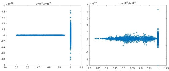
Figure 1. Eigenvalue distribution of preconditioned matrix $P_{Tri}^{-1}\mathcal{A}$.

In Figure 2, the eigenvalue distribution image of preconditioned matrix $P_{Str}^{-1}\mathcal{A}$ with $\epsilon ={10}^{-2}$ is shown.

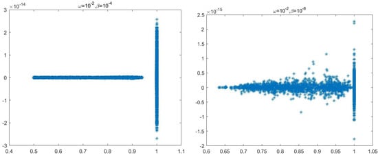
Figure 2. Eigenvalue distribution of preconditioned matrix $P_{Str}^{-1}\mathcal{A}$.

According to Figure 1 and Figure 2, the eigenvalues of the preconditioned matrices $P_{Tri}^{-1}\mathcal{A}$ and $P_{Str}^{-1}\mathcal{A}$ are closer to one for smaller $\beta$’s. This partly explains the reason for the shorter iteration time for smaller $\beta$’s in the numerical calculations. As seen from Figure 1 and Figure 2, all the eigenvalues of the preconditioned matrices are indeed located in the interval $\left[\frac{1}{2},1\right]$, which is consistent with our spectral analyses in Section 4 and Section 5.

7. Conclusions

The purpose of this paper was to construct and analyze the block-triangular preconditioner and structured preconditioner of the discrete linear system of the time-harmonic eddy-current optimal control problem. It was proved that the eigenvalues of their corresponding preconditioned matrices were all located in the interval $\left[\frac{1}{2},1\right]$. Numerical experiments showed that both newly proposed algorithms were robust to the parameters involved in the problem and ran faster than some existing algorithms.

In the future, an extension of our work is to apply new block-triangular preconditioners and structured preconditioners to solve other problems arising in practice, such as the optimal control problem involving the heat equation in [15]. We can further apply this method to compute additional Hermitian operators, addressing problems as referenced in [32]. In addition, we can try to use the newly proposed preconditioners to solve more general algebraic problems with non-Hermite matrices, etc.

References

- Tröltzsch, F. Optimal Control of Partial Differential Equations: Theory, Methods, and Applications; American Mathematical Society: Providence, RI, USA, 2010; Volume 112. [Google Scholar]
- Kolmbauer, M. The Multiharmonic Finite Element and Boundary Element Method for Simulation and Control of Eddy Current Problems. Ph.D. Thesis, Johannes Kepler University, Linz, Austria, 2012. [Google Scholar]
- Lions, J.-L. Optimal Control of Systems Governed by Partial Differential Equations; Springer: Berlin, Germany, 1971. [Google Scholar]
- Ida, N. Numerical Modeling for Electromagnetic Non-Destructive Evaluation; Engineering NDE; Chapman & Halls: London, UK, 1995. [Google Scholar]
- Golub, G.H.; Wu, X.; Yuan, J.-Y. SOR-like methods for augmented systems. Bit Numer. Math. 2001, 41, 71–85. [Google Scholar] [CrossRef]
- Bai, Z.-Z.; Golub, G.H.; Ng, M.K. Hermitian and skew-Hermitian splitting methods for non-Hermitian positive definite linear systems. SIAM J. Matrix Anal. Appl. 2003, 24, 603–626. [Google Scholar] [CrossRef]
- Benzi, M.; Golub, G.H. An iterative method for generalized saddle point problems. SIAM J. Matrix Anal. Appl. 2002, 1–28. [Google Scholar]
- Benzi, M. A generalization of the Hermitian and skew-Hermitian splitting iteration. SIAM J. Matrix Anal. Appl. 2009, 31, 360–374. [Google Scholar] [CrossRef]
- Jiang, M.-Q.; Cao, Y. On local Hermitian and skew-Hermitian splitting iteration methods for generalized saddle point problems. J. Comput. Appl. Math. 2009, 231, 973–982. [Google Scholar] [CrossRef]
- Yang, A.-L.; An, J.; Wu, Y.-J. A generalized preconditioned HSS method for non-Hermitian positive definite linear systems. Appl. Math. Comput. 2010, 216, 1715–1722. [Google Scholar] [CrossRef]
- Bai, Z.-Z. Block alternating splitting implicit iteration methods for saddle-point problems from time-harmonic eddy current models. Numer. Linear Algebra Appl. 2012, 19, 914–936. [Google Scholar] [CrossRef]
- Zheng, Z.; Zhang, G.-F.; Zhu, M.-Z. A block alternating splitting iteration method for a class of block two-by-two complex linear systems. J. Comput. Appl. Math. 2015, 288, 203–214. [Google Scholar] [CrossRef]
- Krendl, W.; Simoncini, V.; Zulehner, W. Stability estimates and structural spectral properties of saddle point problems. Numer. Math. 2013, 124, 183–213. [Google Scholar] [CrossRef]
- Zheng, Z.; Zhang, G.-F.; Zhu, M.-Z. A note on preconditioners for complex linear systems arising from PDE-constrained optimization problems. Appl. Math. Lett. 2016, 61, 114–121. [Google Scholar] [CrossRef]
- Liang, Z.-Z.; Axelsson, O.; Neytcheva, M. A robust structured preconditioner for time-harmonic parabolic optimal control problems. Numer. Algorithms 2018, 79, 575–596. [Google Scholar] [CrossRef]
- Liang, Z.-Z.; Axelsson, O. Exact inverse solution techniques for a class of complex valued block two-by-two linear systems. Numer. Algorithms 2022, 90, 79–98. [Google Scholar] [CrossRef]
- Buffa, A.; Ammari, H.; Nédélec, J.-C. A justification of eddy currents model for the Maxwell equations. SIAM J. Appl. Math. 2000, 60, 1805–1823. [Google Scholar] [CrossRef]
- Schmidt, K.; Sterz, O.; Hiptmair, R. Estimating the eddy-current modeling error. IEEE Trans. Magn. 2008, 44, 686–689. [Google Scholar] [CrossRef]
- Axelsson, O.; Lukáš, D. Preconditioning methods for eddy-current optimally controlled time-harmonic electromagnetic problems. J. Numer. Math. 2019, 27, 1–21. [Google Scholar] [CrossRef]
- Zaglmayr, S. High Order Finite Element Methods for Electromagnetic Field Computation. PhD Thesis, Universität Linz, Linz, Austria, 2006. [Google Scholar]
- Nédélec, J.-C. Mixed finite elements in R3. Numer. Math. 1980, 35, 315–341. [Google Scholar] [CrossRef]
- Nédélec, J.-C. A new family of mixed finite elements in R3. Numer. Math. 1986, 50, 57–81. [Google Scholar] [CrossRef]
- Paige, C.C.; Saunders, M.A. Solution of sparse indefinite systems of linear equations. SIAM J. Numer. Anal. 1975, 12, 617–629. [Google Scholar] [CrossRef]
- Saad, Y.; Schultz, M.H. GMRES: A generalized minimal residual algorithm for solving nonsymmetric linear systems. SIAM J. Sci. Stat. Comput. 1986, 7, 856–869. [Google Scholar] [CrossRef]
- Axelsson, O.; Liang, Z.-Z. A note on preconditioning methods for time-periodic eddy current optimal control problems. J. Comput. Appl. Math. 2019, 352, 262–277. [Google Scholar] [CrossRef]
- Pearson, J.W.; Wathen, A.J. A new approximation of the Schur complement in preconditioners for PDE-constrained optimization. Numer. Linear Algebra Appl. 2012, 19, 816–829. [Google Scholar] [CrossRef]
- Choi, Y.; Farhat, C.; Murray, W.; Saunders, M. A practical factorization of a Schur complement for PDE-constrained distributed optimal control. J. Sci. Comput. 2015, 65, 576–597. [Google Scholar] [CrossRef]
- Hestenes, M.R.; Stiefel, E. Methods of conjugate gradients for solving linear systems. J. Res. Natl. Bur. Stand. 1952, 49, 409–436. [Google Scholar] [CrossRef]
- Rahman, T.; Valdman, J. Fast MATLAB assembly of FEM matrices in 2D and 3D: Nodal elements. Appl. Math. Comput. 2013, 219, 7151–7158. [Google Scholar] [CrossRef]
- Luo, W.-H.; Gu, X.-M.; Carpentieri, B. A dimension expanded preconditioning technique for saddle point problems. BIT Numer. Math. 2022, 62, 1983–2004. [Google Scholar] [CrossRef]
- Luo, W.-H.; Carpentieri, B.; Guo, J. A dimension expanded preconditioning technique for block two-by-two linear equations. Demonstr. Math. 2023, 56, 20230260. [Google Scholar] [CrossRef]
- Gu, X. Efficient preconditioned iterative linear solvers for 3-D magnetostatic problems using edge elements. Adv. Appl. Math. Mech. 2020, 12, 301–318. [Google Scholar] [CrossRef]
Disclaimer/Publisher’s Note: The statements, opinions and data contained in all publications are solely those of the individual author(s) and contributor(s) and not of MDPI and/or the editor(s). MDPI and/or the editor(s) disclaim responsibility for any injury to people or property resulting from any ideas, methods, instructions or products referred to in the content. |
© 2024 by the authors. Licensee MDPI, Basel, Switzerland. This article is an open access article distributed under the terms and conditions of the Creative Commons Attribution (CC BY) license (https://creativecommons.org/licenses/by/4.0/).