Dynamic Asset Allocation and Retirement Decision with Consumption Ratcheting and Effort Choice

Abstract

This study examines the problem of choosing optimal consumption, investment, early retirement, and effort levels for an economic agent who is unwilling to reduce their consumption over time. The agent’s income depends on a fixed wage rate, and varies proportionally with their level of effort, which incurs disutility due to labor. By applying the dual-martingale method, we reformulate the problem into its dual form, dividing it into two distinct sub-problems: one focuses on selecting a consumption path that does not decrease, while the other determines the optimal timing for early retirement. Using this method, we find optimal strategies in the form of explicit closed-form solutions.

1. Introduction

Since Dybvig was awarded the Nobel Prize, one of his earlier works, the consumption ratcheting model in Dybvig [1], has been revisited, and has gained renewed attention. This model addresses the phenomenon where individuals are highly averse to lowering their standard of living once it has increased, emphasizing their tendency to maintain a certain level of consumption. This behavior has significant implications for retirement decisions and long-term financial planning. However, despite the growing interest in the consumption ratcheting framework, key factors such as labor supply, effort choice, and the timing of retirement have not been thoroughly explored.

In practice, individuals face complex decisions regarding their labor supply and work intensity, both of which directly affect their consumption and retirement planning. These factors become particularly important when considering the irreversibility of consumption decisions under a ratcheting constraint. Despite this, most existing models in the literature fail to account for the flexibility in labor effort and its impact on retirement behavior.

Jeon and Park [2] advanced this line of research by addressing the early retirement problem within a consumption ratcheting framework that incorporates the disutility of labor. However, their study did not allow for flexibility in effort choice or labor supply, leaving a gap in understanding how these factors influence optimal retirement strategies.

This paper aims to bridge that gap by incorporating both effort choice and labor flexibility into the consumption ratcheting framework. By allowing individuals to adjust their labor effort and retirement timing, we provide a more comprehensive analysis of how labor decisions interact with consumption and asset allocation under a ratcheting constraint. This contributes to a deeper understanding of optimal strategies for maintaining a desired consumption level while balancing work effort and retirement decisions.

To address this issue, we propose a model based on the consumption ratcheting framework, which integrates early retirement decisions and labor supply adjustments through effort choices. As the agent does not allow any decrease in consumption, the consumption trajectory is assumed to be strictly non-decreasing. The agent may choose an early retirement time, earning income proportional to their effort level at a fixed wage rate until retirement. Once retired, the decision is irreversible, meaning the agent cannot return to work. Additionally, exerting effort incurs a utility cost, represented by a convex function.

This problem introduces notable challenges, as the agent must simultaneously optimize, over a non-decreasing consumption trajectory, the timing of early retirement, an investment strategy, and the effort level. Consequently, solving the utility maximization problem requires the integration of stochastic control, singular control, and optimal stopping techniques.

To address this challenge, we utilize the dual-martingale approach to reformulate the agent’s problem into a dual framework. The additive structure of the utility cost allows the dual problem to be decomposed into two parts: a singular control for consumption, and an optimal stopping for early retirement. By solving these components independently, we derive explicit solutions for the dual problem. Additionally, a strong duality theorem is established, connecting the dual and primal problems and providing a characterization of the agent’s optimal strategies.

Earlier research has thoroughly explored early retirement and consumption ratcheting within continuous-time consumption and investment models (see, for instance, Choi and Shim [3], Choi et al. [4], Yang and Koo [5], Ivanov and Tian [6], Dybvig [1], Jeon et al. [7], Jeon et al. [8], Jeon and Park [2], Jeon and Park [9], and other related works). Our contribution to the literature lies in integrating these aspects by combining consumption ratcheting, early retirement, and labor supply through effort choices into a unified framework.

Additionally, our paper is closely related to the literature on consumption constraints (e.g., Abel [10], Chetty and Szeidl [11], Chetty and Szeidl [12], Detemple and Zapatero [13], Guasoni et al. [14], Deng et al. [15], van Bilsen et al. [16], and reference therein). Among them, we modeled the agent’s preference as consumption ratcheting, which is an extreme form of consumption habit.

Organization: Section 2 introduces the framework, which integrates early retirement, consumption ratcheting, and labor supply adjustments through effort choices. In Section 3, we formulate the dual problem and decompose it into two sub-problems: one focusing on the optimization of a non-decreasing consumption plan, and the other on identifying the optimal timing for early retirement. This section also characterizes the solutions to these sub-problems. Section 4 establishes a strong duality theorem, and provides a detailed characterization of the agent’s optimal strategy.

2. Model

We consider a financial market that operates in continuous time and consists of two primary assets: a risk-free asset with interest rate $r>0$ (here, r is constant), and a risky asset referred to as the stock ${\left(S_t\right)}_{t\ge 0}$.

The dynamics of $S_t$ are modeled by

$${\displaystyle \frac{d{S}_t}{S_t}}=\mu dt+\sigma d{B}_t,$$

where $\mu \ne r$ and $\sigma >0$ are constants, and ${\left(B_t\right)}_{t\ge 0}$ is a standard Brownian motion defined on the filtered probability space $(\Omega ,\mathcal{F},\mathbb{F},\mathbb{P})$. The filtration $\mathbb{F}$ is the usual augmentation of the natural filtration generated by ${\left(B_t\right)}_{t\ge 0}$.

Following the methodology of Dybvig [1], we investigate a setting where the agent prefers a non-decreasing consumption path. Let $c_t$ represent the agent’s consumption at time t. The consumption process ${\left(c_t\right)}_{t\ge 0}$ is assumed to belong to the admissible set $\Pi \left(c\right)$. The set $\Pi \left(c\right)$ consists of all $\mathbb{F}$-adapted, positive, right-continuous with left limits (RCLL), and non-decreasing processes that start with the initial value c.

Additionally, the agent receives income from labor and can choose an early retirement date, $\tau$, at any time. However, the early retirement option is irreversible, meaning that once the agent retires early, they cannot return to work. The agent earns wage income proportional to their effort, $e_t$, at a rate of $w{e}_t$ at time t, where $w>0$ is the constant wage per unit of effort. Effort can be interpreted as working hours, work intensity, or both. The agent can choose effort within a bounded interval: for every $t\ge 0$,

$$\begin{array}{c}\hfill 0<L\le e_t\le H.\end{array}$$

(1)

where L and H are fixed constants. The upper bound H corresponds to physical and/or psychological limit for effort when working. The lower bound L means that there exists a technological constraint on the effort level for work to be productive; work with an effort level lower than L is not productive.

Let ${\pi }_t$ represent the investment made by the agent in $S_t$ at time t. The evolution of the agent’s wealth process $X_t$ follows the dynamics given by:

$$d{X}_t=\left[(\mu -r){\pi }_t+r{X}_t-c_t+w{e}_t{\mathbf{1}}_{\{t<\tau \}}\right]dt+\sigma {\pi }_{t}d{B}_t,X_0=x,$$

(2)

with $X_0=x$.

The agent’s preference is expressed by

$$U:=\mathbb{E}\left[{\int }_0^{\tau }{e}^{-\rho t}\left(u\left(c_t\right)-h\left(e_t\right)\right)dt+{\int }_{\tau }^{\infty }{e}^{-\rho t}u\left(c_t\right)dt\right].$$

(3)

Here, $\rho >0$ is the subjective discount rate, $u:(0,\infty )\to \mathbb{R}$ is the felicity function for consumption, and $h\left(e_t\right)$ represents the utility cost of effort at time t.

To ensure the well-definedness, and to make the problem meaningful, we impose the following assumptions on utility u and cost h:

Assumption 1. 

$h:[0,\infty )\to (0,\infty )$ is $C^2$ with $h\left(0\right)=0$. Moreover, $h^{\prime }>0$ and $h^{\prime \prime }>0$ in $y>0$.

Remark 1. 

Defining utility cost function h of effort as increasing and convex is reasonable because higher effort requires greater incremental costs due to physical and mental limitations. This structure reflects realistic decision-making, ensures mathematical stability in optimization, and aligns with observed behaviors like diminishing returns to effort.

Assumption 2. 

$u:(0,\infty )\to [-\infty ,\infty )$ is $C^2$. Additionally, $u^{\prime }>0$ and $u^{\prime \prime }<0$ in $y>0$, and u satisfies the following conditions:

$$\underset{c\to +\infty }{lim}{u}^{\prime }\left(c\right)=0,\mathit{and}\underset{c\to 0+}{lim}{u}^{\prime }\left(c\right)=\infty .$$

Remark 2. 

Assumption 3 is the commonly used Inada condition frequently assumed in the economics literature. The Inada conditions ensure that marginal utility approaches infinity as consumption approaches zero and zero as consumption approaches infinity, promoting interior solutions in optimization problems.

Assumption 3. 

For $y>0$, the integral below is assumed to converge:

$${\int }_0^y{\eta }^{-n_2}I\left(\eta \right)d\eta <\infty .$$

Here, $n_1>0$ and $n_2<0$ are two solutions to the following quadratic equation: ${\displaystyle \frac{{\theta }^2}{2}}n(n-1)+\left(\beta -r\right)n-\beta =0.$

Remark 3. 

Assumption 3 ensures the well-definedness of the value function in our optimization problem, as it is set in an infinite horizon framework. For further details, refer to Karatzas and Shreve [17] (Theorem 9.14).

Problem 1. 

Let $c>0$ and $x>(c-wH)/r$ be given. The agent’s value function is defined as

$$V\left(x\right)=\underset{(c,\pi ,\tau ,e)\in \mathcal{A}(x,c)}{sup}\mathbb{E}\left[{\int }_0^{\tau }{e}^{-\rho t}\left(u\left(c_t\right)-h\left(e_t\right)\right)dt+{\int }_{\tau }^{\infty }{e}^{-\rho t}u\left(c_t\right)dt\right],$$

(4)

where $\mathcal{A}(x,c)$ represents the collection of all admissible strategies, subject to the following constraints:

(i) 

${\left(c_t\right)}_{t\ge 0}\in \Pi \left(c\right)$;

(ii) 

${\left(e_t\right)}_{t\ge 0}$ is a $\mathbb{F}$-adapted positive process such that $L\le e_t\le H$ for all $t\ge 0$ and ${\int }_0^t{e}_{s}ds<\infty$ almost surely;

(iii) 

${\pi }_t$ is an $\mathbb{F}$-progressively measurable process with ${\int }_0^t{\pi }_s^{2}ds<\infty$,

(iv) 

$\tau \in \mathcal{S}$. Here, $\mathcal{S}$ is the family of all $\mathbb{F}$-stopping times that take values in $[0,\infty ]$;

(v) 

The wealth process $X_t^{c,\pi ,\tau ,e}$, associated with the strategy $(c,\pi ,\tau ,e)$, satisfies the natural wealth constraint:

$$X_t\ge {\displaystyle \frac{c_t}{r}}-{\displaystyle \frac{wH}{r}}{\mathbf{1}}_{\{t<\tau \}}.$$

3. Optimization Problem

Problem 1 requires identifying an increasing consumption $c_t$, selecting the optimal retirement time $\tau$, and determining the suitable effort level $e_t$. To tackle the complexities of this problem, we employ the dual-martingale approach.

As part of this framework, we introduce the stochastic discount factor (SDF) $H_t$, defined as

$$H_t:=e^{-(r+{\displaystyle \frac{1}{2}}{\theta }^2)t-\theta B_t},\mathrm{where}\theta :={\displaystyle \frac{\mu -r}{\sigma }}.$$

(5)

Using the SDF, the wealth dynamics Equation (2) can be reformulated as the following constraint:

$$\mathbb{E}\left[{\int }_0^{\tau }{H}_t\left(c_t-w{e}_t\right)dt+{\int }_{\tau }^{\infty }{H}_t{c}_{t}dt\right]\le x.$$

(6)

We define the Lagrangian $\mathfrak{L}$. For a given $(c,\pi ,\tau ,e)\in \mathcal{A}(x,c)$, the Lagrangian is represented as:

$$\begin{array}{cc}\hfill \mathfrak{L}=& \mathbb{E}\left[{\int }_0^{\tau }{e}^{-\rho t}\left(u\left(c_t\right)-h\left(e_t\right)\right)dt+{\int }_{\tau }^{\infty }{e}^{-\rho t}u\left(c_t\right)dt\right]\hfill \\ \hfill & +y\left(x-\mathbb{E}\left[{\int }_0^{\tau }{H}_t\left(c_t-w{e}_t\right)dt+{\int }_{\tau }^{\infty }{H}_t{c}_{t}dt\right]\right)\hfill \\ \hfill =& \mathbb{E}\left[{\int }_0^{\infty }{e}^{-\rho t}\left(u\left(c_t\right)-Y_t^y{c}_t\right)dt\right]+\mathbb{E}\left[{\int }_0^{\tau }{e}^{-\rho t}\left(w{e}_t{Y}_t^y-h\left(e_t\right)\right)dt\right]+yx\hfill \\ \hfill \le & \mathbb{E}\left[{\int }_0^{\infty }{e}^{-\rho t}\left(u\left(c_t\right)-Y_t^y{c}_t\right)dt\right]+\mathbb{E}\left[{\int }_0^{\tau }{e}^{-\rho t}\tilde{h}\left(Y_t^y\right)dt\right]+yx.\hfill \end{array}$$

(7)

Here, $y>0$ is the initial Lagrange multiplier for (6), $Y_t^y:=y{e}^{\rho t}{H}_t$, and $\tilde{h}(·)$ is defined as follows:

$$\begin{array}{cc}\hfill \tilde{h}\left(y\right)=& \underset{L\le e\le H}{sup}\left(wye-h\left(e\right)\right)\hfill \\ \hfill =& \left(wyL-h\left(L\right)\right){\mathbf{1}}_{\{y\le h^{\prime }\left(L\right)/w\}}+\left(wy{I}_h\left(wy\right)-h\left(I_h\left(wy\right)\right)\right){\mathbf{1}}_{\{h^{\prime }\left(L\right)/w<y\le h^{\prime }\left(H\right)/w\}}\hfill \\ \hfill & +\left(wyH-h\left(H\right)\right){\mathbf{1}}_{\{y>h^{\prime }\left(H\right)/w\}}.\hfill \end{array}$$

(8)

Here, $I_h\left(y\right)$ represents the inverse of $h^{\prime }$ over the domain $(0,\infty )$.

The inequality in (7) holds an equality if and only if the following holds for the effort level $e_t$:

$$\begin{array}{c}\hfill e_t=\widehat{e}\left(Y_t^y\right):=\left\{\begin{array}{cc}L\hfill & \mathrm{if}{Y}_t^y\le {\displaystyle \frac{h^{\prime }\left(L\right)}{w}},\hfill \\ I_h\left(Y_t^y\right)\hfill & \mathrm{if}{\displaystyle \frac{h^{\prime }\left(L\right)}{w}}<Y_t^y<{\displaystyle \frac{h^{\prime }\left(H\right)}{w}},\hfill \\ H\hfill & \mathrm{if}{Y}_t^y\ge {\displaystyle \frac{h^{\prime }\left(H\right)}{w}}.\hfill \end{array}\right.\end{array}$$

(9)

We now define the functions $J_A(y,c)$, $J_R\left(y\right)$, and $J(y,c)$ as follows:

$$\begin{array}{cc}\hfill J_A(y,c):=& \underset{\left(c_t\right)\in \Pi \left(c\right)}{sup}\mathbb{E}\left[{\int }_0^{\infty }{e}^{-\rho t}\left(u\left(c_t\right)-Y_t^y{c}_t\right)dt\right],\hfill \\ \hfill J_R\left(y\right):=& \underset{\tau \in \mathcal{S}}{sup}\mathbb{E}\left[{\int }_0^{\tau }{e}^{-\rho t}\tilde{h}\left(Y_t^y\right)dt\right],\hfill \end{array}$$

(10)

and

$$J(y,c):=J_A(y,c)+J_R\left(y\right).$$

(11)

Using the Lagrangian $\mathfrak{L}$, we establish the weak duality property: for any $(c,\pi ,\tau ,e)\in \mathcal{A}(x,c)$, the following inequality holds:

$$V(x,c)\le \underset{y>0}{inf}\left[J(y,c)+yx\right].$$

(12)

Here, $J(y,c)$ is referred to as the dual value function. By its definition, $J(y,c)$ is decomposed into two distinct sub-problems. The first sub-problem involves determining the non-decreasing consumption process, $\left(c_t\right)$, while the second focuses on selecting the optimal retirement time, $\tau$. The separability of these problems arises due to the additive structure of the disutility in the dual problem. Specifically, the consumption decision and the retirement timing are independent in the dual formulation. In contrast, these two components are interdependent in the primal problem, where decisions about consumption and retirement timing influence each other.

3.1. Sub-Problem I: Optimal Retirement Decision

We begin by analyzing the sub-problem associated with $J_R\left(y\right)$, which determines the optimal retirement time for the agent.

By applying a theory of optimal stopping, we consider the following variational inequality (VI) of $J_R\left(y\right)$:

$$max\left\{{\displaystyle \frac{{\theta }^2}{2}}{y}^2{J}_R^{\prime \prime }\left(y\right)+(\rho -r)y{J}_R^{\prime }\left(y\right)-\rho J_R+\tilde{h}\left(y\right),-J_R\left(y\right)\right\}=0.$$

(13)

There exists a critical threshold $z_R$, such that

$$\left\{\begin{array}{c}{\displaystyle \frac{{\theta }^2}{2}}{y}^2{J}_R^{\prime \prime }\left(y\right)+(\rho -r)y{J}_R^{\prime }\left(y\right)-\rho J_R+\tilde{h}\left(y\right)=0\mathrm{for}y>z_R,\hfill \\ J_R\left(y\right)=0\mathrm{for}0<y\le z_R.\hfill \end{array}\right.$$

(14)

The smooth pasting condition provides the following boundary conditions:

$$J_R\left(z_R\right)=J_R^{\prime }\left(z_R\right)=0,J_R\left(y\right)=0\mathrm{for}0<y\le z_R.$$

(15)

To guarantee that the solution to the VI (13), we impose the following transversality condition:

$$\underset{t\to \infty }{lim}{e}^{-\rho t}\mathbb{E}\left[J_R\left(Y_t^y\right)\right]=0.$$

(16)

For $y>z_R$, the general solution to $J_R\left(y\right)$ is composed of a combination of the homogeneous solution and a particular solution,

$$J_R\left(y\right)=D{y}^{n_2}+{\Psi }_p\left(y\right),$$

(17)

where the particular solution ${\Psi }_p\left(y\right)$ is

$${\Psi }_p\left(y\right)=\left[y^{n_2}{\int }_0^y{\nu }^{-n_2-1}\tilde{h}\left(\nu \right)d\nu +y^{n_1}{\int }_y^{\infty }{\nu }^{-n_1-1}\tilde{h}\left(\nu \right)d\nu \right]{\displaystyle \frac{2}{{\theta }^2(n_1-n_2)}}.$$

(18)

To satisfy the transversality condition (16), the term involving $y^{n_1}$ in (17) is excluded.

Remark 4. 

The homogeneous equation corresponding to (13) is given by

$${\displaystyle \frac{{\theta }^2}{2}}{y}^2{\left(J_R^{\mathit{hom}}\right)}^{\prime \prime }\left(y\right)+(\rho -r)y{\left(J_R^{\mathit{hom}}\right)}^{\prime }\left(y\right)-\rho J_R^{\mathit{hom}}=0.$$

(19)

Assuming a solution of the form $J_R^{\mathit{hom}}\left(y\right)=y^n$, the characteristic equation becomes

$${\displaystyle \frac{{\theta }^2}{2}}n(n-1)+(\rho -r)n-\rho =0,$$

(20)

which yields two roots, $n_1>0$ and $n_2<0$. The general solution to the homogeneous equation is, therefore,

$$J_R^{\mathit{hom}}\left(y\right)=C_1{y}^{n_1}+C_2{y}^{n_2}.$$

(21)

In the general solution for $J_R\left(y\right)$ in (17), the transversality condition (16) requires

$$\underset{t\to \infty }{lim}{e}^{-\rho t}\mathbb{E}\left[J_R\left(Y_t^y\right)\right]=0.$$

(22)

This condition ensures that $J_R\left(y\right)$ does not grow exponentially as $y\to \infty$. Since $y^{n_1}$ grows unbounded as $y\to \infty$, the term involving $y^{n_1}$ must be excluded ($C_1=0$). As a result, the general solution simplifies to

$$J_R\left(y\right)=D{y}^{n_2}+{\Psi }_p\left(y\right),$$

(23)

where $y^{n_2}$ vanishes as $y\to \infty$, satisfying the transversality condition.

By applying the smooth pasting condition (15), we deduce that there is a unique $z_R\in (0,{\displaystyle \frac{h\left(L\right)}{wL}})$, such that:

$${\int }_{z_R}^{\infty }{\nu }^{-n_1-1}\tilde{h}\left(\nu \right)d\nu =0\mathrm{and}D=-{\displaystyle \frac{2}{{\theta }^2(n_1-n_2)}}{\int }_0^{z_R}{\nu }^{-n_2-1}\tilde{h}\left(\nu \right)d\nu .$$

(24)

Proposition 1. 

The option value of voluntary retirement, $J_R\left(y\right)$, is expressed as

$$J_R\left(y\right)=\left\{\begin{array}{cc}D{y}^{n_2}+{\Psi }_p\left(y\right)\hfill & \mathit{for}y\ge z_R,\hfill \\ 0\hfill & \mathit{for}0<y\le z_R.\hfill \end{array}\right.$$

(25)

$J_R\left(y\right)$ is $C^1(0,\infty )$ and strictly convex function of $y>0$. Also, ${\tau }_R\left(y\right)$, the optimal stopping time in $J_R\left(y\right)$, is given by

$${\tau }_R\left(y\right)=inf\{t\ge 0\mid Y_t^y\le z_R\}.$$

Proof. 

Define $\mathcal{G}\left(y\right)$ as

$$\begin{array}{c}\hfill \mathcal{G}\left(y\right)={\int }_y^{\infty }{\nu }^{-n_1-1}\tilde{h}\left(\nu \right)d\nu .\end{array}$$

Using the strict convexity of h and the condition $h\left(0\right)=0$, it follows that

$$h\left(0\right)>h\left(L\right)-h^{\prime }\left(L\right)L,\mathrm{or} \mathrm{equivalently}h\left(L\right)<h^{\prime }\left(L\right)L.$$

(26)

Since $\tilde{h}\left(y\right)>0$ for $y>{\displaystyle \frac{h\left(L\right)}{wL}}$, and

$$\begin{array}{c}\hfill \underset{y\to 0+}{lim}\left[{\displaystyle \frac{y^{1-n_1}}{n_1-1}}wL-{\displaystyle \frac{y^{-n_1}}{n_1}}h\left(L\right)\right]=\underset{y\to 0+}{lim}{\displaystyle \frac{y^{-n_1}}{n_1-1}}L\left(wy-(n_1-1){\displaystyle \frac{1}{n_1}}{\displaystyle \frac{h\left(L\right)}{L}}\right)=-\infty ,\end{array}$$

we obtain

$$\mathcal{G}\left({\displaystyle \frac{h\left(L\right)}{wL}}\right)>0\mathrm{and}\mathcal{G}(0+)=-\infty .$$

For $0<y<{\displaystyle \frac{h\left(L\right)}{wL}}$, the derivative of $\mathcal{G}\left(y\right)$ is given by

$${\mathcal{G}}^{\prime }\left(y\right)=-y^{-n_1-1}\tilde{h}\left(y\right)=-\left(wyL-h\left(L\right)\right)>0.$$

By applying the intermediate value theorem, we deduce the existence of a unique $z_R\in (0,{\displaystyle \frac{h\left(L\right)}{wL}})$, such that

$$\mathcal{G}\left(z_R\right)=0.$$

As a result, the parameter D is determined as follows:

$$D=-{\displaystyle \frac{2}{{\theta }^2(n_1-n_2)}}{\int }_0^{z_R}{\nu }^{-n_2-1}\tilde{h}\left(\nu \right)d\nu =-{\displaystyle \frac{2}{{\theta }^2(n_1-n_2)}}\left[wL{\displaystyle \frac{z_R^{1-n_2}}{1-n_2}}+L^2{\displaystyle \frac{z_R^{-n_2}}{2n_2}}\right].$$

(27)

The remaining parts are proved in the following three steps:

Step 1: $J_R\left(y\right)$ in (25) is strictly convex and strictly increasing for $y\in (z_R,\infty )$.

Proof of Step 1. We can rewrite the form of $J_R\left(y\right)$ as follows:

$$\begin{array}{cc}\hfill J_R\left(y\right)=& \left[-{\displaystyle \frac{2}{{\theta }^2(n_1-n_2)}}{\int }_0^{z_R}{\nu }^{-n_2-1}\tilde{h}\left(\nu \right)d\nu \right]y^{n_2}\hfill \\ \hfill & +{\displaystyle \frac{2}{{\theta }^2(n_1-n_2)}}\left[y^{n_2}{\int }_0^y{\nu }^{-n_2-1}\tilde{h}\left(\nu \right)d\nu +y^{n_1}{\int }_y^{\infty }{\nu }^{-n_1-1}\tilde{h}\left(\nu \right)d\nu \right]\hfill \\ \hfill =& {\displaystyle \frac{2}{{\theta }^2(n_1-n_2)}}\left[y^{n_2}{\int }_{z_R}^y{\nu }^{-n_2-1}\tilde{h}\left(\nu \right)d\nu +y^{n_1}{\int }_y^{\infty }{\nu }^{-n_1-1}\tilde{h}\left(\nu \right)d\nu \right].\hfill \end{array}$$

For $y>z_R$, the derivative $J_R^{\prime }\left(y\right)$ is

$$\begin{array}{cc}\hfill J_R^{\prime }\left(y\right)=& \left[n_2{y}^{n_2-1}{\int }_{z_R}^y{\nu }^{-n_2-1}\tilde{h}\left(\nu \right)d\nu +n_1{y}^{n_1-1}{\int }_y^{\infty }{\nu }^{-n_1-1}\tilde{h}\left(\nu \right)d\nu \right]{\displaystyle \frac{2}{{\theta }^2(n_1-n_2)}}\hfill \\ \hfill =& \left[y^{n_2-1}{z}_R^{-n_2}\tilde{h}\left(z_R\right)+y^{n_2-1}{\int }_{z_R}^y{\nu }^{-n_2}{\tilde{h}}^{\prime }\left(\nu \right)d\nu +y^{n_1-1}{\int }_y^{\infty }{\nu }^{-n_1}{\tilde{h}}^{\prime }\left(\nu \right)d\nu \right]{\displaystyle \frac{2}{{\theta }^2(n_1-n_2)}},\hfill \end{array}$$

where integration by parts has been applied, and we use

$$\underset{y\to \infty }{lim}{\nu }^{-n_1}\tilde{h}\left(\nu \right)=0.$$

Similarly, for $y>z_R$, the second derivative $J_R^{\prime \prime }\left(y\right)$ is given by

$$\begin{array}{cc}\hfill J_R^{\prime \prime }\left(y\right)=& \left[(n_2-1)y^{n_2-2}{z}_R^{-n_2}\tilde{h}\left(z_R\right)+(n_2-1)y^{n_2-2}{\int }_{z_R}^y{\nu }^{-n_2}{\tilde{h}}^{\prime }\left(\nu \right)d\nu \right.\hfill \\ \hfill & \left.+(n_1-1)y^{n_1-2}{\int }_y^{\infty }{\nu }^{-n_1}{\tilde{h}}^{\prime }\left(\nu \right)d\nu \right]{\displaystyle \frac{2}{{\theta }^2(n_1-n_2)}},\hfill \end{array}$$

where we have applied integration by parts to the Riemann–Stieltjes integrals, along with the condition

$$\underset{y\to \infty }{lim}{\nu }^{1-n_1}{\tilde{h}}^{\prime }\left(\nu \right)=0.$$

Since $h^{\prime }\left(\nu \right)$ is non-decreasing, the Riemann–Stieltjes integrals remain non-negative. Furthermore,

$$(n_2-1)y^{n_2-2}{z}_R^{-n_2}\tilde{h}\left(z_R\right)>0,y^{n_2-1}{z}_R^{1-n_2}{\tilde{h}}^{\prime }\left(z_R\right)>0.$$

Thus, $J_R\left(y\right)$ is strictly convex for $y\in (z_R,\infty )$.

Given that $J_R^{\prime }\left(z_R\right)=0$, it follows that

$$J_R^{\prime }\left(y\right)>0\mathrm{for}y>z_R.$$

Step 2: The function $J_R\left(y\right)$ satisfies the variational inequality given by

$$\left\{\begin{array}{cc}\mathcal{L}{J}_R\left(y\right)+\tilde{h}\left(y\right)\le 0\hfill & \mathrm{if}{J}_R\left(y\right)=0,\hfill \\ \mathcal{L}{J}_R\left(y\right)+\tilde{h}\left(y\right)=0\hfill & \mathrm{if}{J}_R\left(y\right)>0,\hfill \end{array}\right.$$

(28)

where

$$\mathcal{L}={\displaystyle \frac{{\theta }^2}{2}}{y}^2{\displaystyle \frac{d^2}{d{y}^2}}+(\rho -r)y{\displaystyle \frac{d}{dy}}-\rho .$$

Proof of Step 2. Since $J_R\left(z_R\right)=0$, it follows from Step 1 that

$$\{y>0\mid J_R\left(y\right)=0\}=\{y>0\mid 0<y\le z_R\},\{y>0\mid J_R\left(y\right)>0\}=\{y>0\mid z_R<y\}.$$

Clearly,

$$\mathcal{L}{J}_R\left(y\right)+\tilde{h}\left(y\right)=0\mathrm{for}y>z_R.$$

Since $\tilde{h}\left(y\right)<0$ and $J_R\left(y\right)=0$ for $y\in (0,z_R)$, we have

$$\mathcal{L}{J}_R\left(y\right)+\tilde{h}\left(y\right)=\tilde{h}\left(y\right)\le 0\mathrm{for}0<y\le z_R.$$

Combining these, $J_R\left(y\right)$ satisfies the stated variational inequality.

Step 3: $J_R\left(y\right)$ in (25) satisfies the following properties:

(i)

$J_R(·)\in {\mathcal{W}}_{\mathrm{loc}}^{2,p}(0,\infty )$.

(ii)

${lim\; inf}_{t\to \infty }{e}^{-\rho t}\mathbb{E}\left[J_R\left(Y_t^y\right)\right]=0$.

(iii)

For all fixed $T>0$, the process

$${\mathcal{N}}_t={\int }_0^{T\wedge t}{e}^{-\rho s}\theta Y_s^y{J}_R^{\prime }\left(Y_s^y\right)ds$$

is a martingale.

Using Steps 1, 2, and 3, we conclude from Knudsen et al. [18] (Theorem 3.2) that

$$J_R\left(y\right)=\underset{\tau \in \mathcal{S}}{sup}\mathbb{E}\left[{\int }_0^{\tau }{e}^{-\rho t}\tilde{h}\left(Y_t^y\right)dt\right]=\mathbb{E}\left[{\int }_0^{{\tau }_R\left(y\right)}{e}^{-\rho t}\tilde{h}\left(Y_t^y\right)dt\right],$$

where

$${\tau }_R\left(y\right)=inf\{t\ge 0\mid Y_t^y\le z_R\}.$$

□

Lemma 1. 

The following limiting behaviors hold:

$$\underset{y\to \infty }{lim}{J}_R^{\prime }\left(y\right)={\displaystyle \frac{wH}{r}},\mathit{and}\underset{y\to 0+}{lim}{J}_R^{\prime }\left(y\right)=0.$$

Proof. 

It is clear that

$$\underset{y\to 0+}{lim}{J}_R^{\prime }\left(y\right)=0.$$

By Knudsen et al. [18] (Proposition 4.1),

$$\underset{y\downarrow 0}{lim\; inf}|\tilde{h}\left(y\right)|y^{-n_2}=0,\mathrm{and}\underset{y\uparrow \infty }{lim\; inf}\left|\tilde{h}\left(y\right)\right|y^{-n_1}=0.$$

By applying integration by parts, we obtain

$${\Psi }_p^{\prime }\left(y\right)={\displaystyle \frac{2}{{\theta }^2(n_1-n_2)}}\left[y^{n_2-1}{\int }_0^y{\nu }^{-n_2}{\tilde{h}}^{\prime }\left(\nu \right)d\nu +y^{n_1-1}{\int }_y^{\infty }{\nu }^{-n_1}{\tilde{h}}^{\prime }\left(\nu \right)d\nu \right].$$

Since ${\tilde{h}}^{\prime }\left(\nu \right)$ is bounded for $\nu >0$, the term involving $y^{n_2-1}$ vanishes as $y\to \infty$. Consequently,

$$\underset{y\to \infty }{lim}{\Psi }_p^{\prime }\left(y\right)={\displaystyle \frac{2}{{\theta }^2(n_1-n_2)}}\left[{\displaystyle \frac{wH}{1-n_2}}-{\displaystyle \frac{wH}{1-n_1}}\right]={\displaystyle \frac{wH}{r}}.$$

Hence,

$$\underset{y\to \infty }{lim}{J}_R^{\prime }\left(y\right)={\displaystyle \frac{wH}{r}}.$$

□

Lemma 2. 

For $y>0$, the following equality holds:

$$J_R^{\prime }\left(y\right)=\mathbb{E}\left[{\int }_0^{{\tau }_R\left(y\right)}w\widehat{e}\left(Y_t^y\right)dt\right],$$

where $\widehat{e}(·)$ is defined in (9).

Proof. 

For $y>z_R$, the smoothness of $J_R\left(y\right)$ implies

$${\displaystyle \frac{{\theta }^2}{2}}{y}^2{J}_R^{\prime \prime \prime }\left(y\right)+(\rho -r+{\theta }^2)y{J}_R^{\prime \prime }\left(y\right)-r{J}_R^{\prime }\left(y\right)+h^{\prime }\left(y\right)=0.$$

By utilizing the generalized Itô’s lemma to $J_R^{\prime }\left(Y_t^y\right)$, we obtain

$$d{J}_R^{\prime }\left(Y_t^y\right)=\left[r{J}_R^{\prime }\left(Y_t^y\right)-\widehat{e}\left(Y_t^y\right){\mathbf{1}}_{\{t<{\tau }_R\left(y\right)\}}\right]dt-\theta Y_t^y{J}_R^{\prime \prime }\left(Y_t^y\right)d{B}_t^{\mathbb{Q}},$$

where $\mathbb{Q}$ is a risk-neutral measure with $B_t^{\mathbb{Q}}=B_t+\theta t$.

Let $M_t=e^{-rt}{J}_R^{\prime }\left(Y_t^y\right)$. Then,

$$d{M}_t=-e^{-rt}\widehat{e}\left(Y_t^y\right){\mathbf{1}}_{\{t<{\tau }_R\left(y\right)\}}dt-e^{-rt}\theta Y_t^y{J}_R^{\prime \prime }\left(Y_t^y\right)d{B}_t^{\mathbb{Q}}.$$

Taking expectations under $\mathbb{Q}$, and noting that the terminal term vanishes due to the transversality condition, we obtain

$$J_R^{\prime }\left(y\right)=\mathbb{E}\left[{\int }_0^{\infty }{e}^{-rt}\widehat{e}\left(Y_t^y\right){\mathbf{1}}_{\{t<{\tau }_R\left(y\right)\}}dt\right].$$

□

3.2. Sub-Problem II: Adjusting Consumption

In this subsection, we explore the optimal adjustment of consumption, building upon related discussions in Jeon et al. [8] and Jeon and Park [2]. For clarity, we summarize the key ideas and results without delving into exhaustive detail.

For any $\xi >0$, the inverse mapping ${\tau }^{\xi }$, defined for a right-continuous non-decreasing consumption process $c_t$, is expressed as

$${\tau }^{\xi }:=inf\{t\ge 0\mid c_t\ge \xi \}.$$

(29)

Exploiting the one-to-one correspondence between the consumption path ${\left(c_t\right)}_{t\ge 0}$ and its inverse ${\left({\tau }^{\xi }\right)}_{\xi >0}$, we derive the following:

$$\begin{array}{cc}\hfill & \mathbb{E}\left[{\int }_0^{\infty }{e}^{-\rho t}\left(u\left(c_t\right)-Y_t^y{c}_t\right)dt\right]\hfill \\ \hfill =& \mathbb{E}\left[{\int }_0^{\infty }{e}^{-\rho t}\left(u\left(c\right)-Y_t^{y}c\right)dt\right]+\mathbb{E}\left[{\int }_0^{\infty }{\int }_c^{c_t}\left(u^{\prime }\left(\xi \right)-Y_t^y\right)d\xi dt\right]\hfill \\ \hfill =& {\displaystyle \frac{u\left(c\right)}{\rho }}-{\displaystyle \frac{yc}{r}}+\mathbb{E}\left[{\int }_0^{\infty }{\int }_c^{\infty }\left(u^{\prime }\left(\xi \right)-Y_t^y\right){\mathbb{I}}_{\{c_t\ge \xi \}}d\xi dt\right]\hfill \\ \hfill =& {\displaystyle \frac{u\left(c\right)}{\rho }}-{\displaystyle \frac{yc}{r}}+{\int }_c^{\infty }\mathbb{E}\left[{\int }_0^{\infty }\left(u^{\prime }\left(\xi \right)-Y_t^y\right){\mathbb{I}}_{\{{\tau }^{\xi }\le t\}}dt\right]d\xi \hfill \\ \hfill =& {\displaystyle \frac{u\left(c\right)}{\rho }}-{\displaystyle \frac{yc}{r}}+{\int }_c^{\infty }{u}^{\prime }\left(\xi \right)\mathbb{E}\left[{\int }_{{\tau }^{\xi }}^{\infty }\left(1-{\displaystyle \frac{Y_t^y}{u^{\prime }\left(\xi \right)}}\right)dt\right]d\xi .\hfill \end{array}$$

(30)

The optimization problem can be represented as

$$\mathcal{Q}\left(z\right):=\underset{\tau \in \mathcal{S}}{sup}\mathbb{E}\left[{\int }_{\tau }^{\infty }{e}^{-\rho t}\left(1-Y_t^z\right)dt\right].$$

(31)

As shown in Jeon et al. [8] and Jeon and Park [2], the following relationship holds:

$$J_A(y,c)=\underset{\left(c_t\right)\in \Pi \left(c\right)}{sup}\mathbb{E}\left[{\int }_0^{\infty }{e}^{-\rho t}\left(u\left(c_t\right)-Y_t^y{c}_t\right)dt\right]={\int }_c^{\infty }{u}^{\prime }\left(\xi \right)\mathcal{Q}\left({\displaystyle \frac{y}{u^{\prime }\left(\xi \right)}}\right)d\xi +{\displaystyle \frac{u\left(c\right)}{\rho }}-{\displaystyle \frac{yc}{r}}.$$

(32)

Using the optimal stopping theory, we consider the variational inequality of $\mathcal{Q}\left(z\right)$ as follows:

$$\begin{array}{c}\hfill \left\{\begin{array}{cc}\mathcal{L}\mathcal{Q}=0\hfill & \mathrm{if}\mathcal{Q}\left(z\right)>{\displaystyle \frac{1}{\rho }}-{\displaystyle \frac{z}{r}},\hfill \\ \mathcal{L}\mathcal{Q}\le 0\hfill & \mathrm{if}\mathcal{Q}\left(z\right)={\displaystyle \frac{1}{\rho }}-{\displaystyle \frac{z}{r}},\hfill \end{array}\right.\end{array}$$

(33)

alongside the transversality condition,

$$\underset{t\to \infty }{lim}\mathbb{E}\left[\mathcal{Q}\left(Y_t^z\right)\right]=0.$$

(34)

Here, $\mathcal{L}$ is defined as

$$\mathcal{L}\zeta \left(z\right):={\displaystyle \frac{{\theta }^2}{2}}{z}^2{\zeta }^{\prime \prime }\left(z\right)+(\rho -r)z{\zeta }^{\prime }\left(z\right)-\rho \zeta \left(z\right).$$

(35)

Using an approach analogous to the one applied in the proof of Proposition 1, it can be shown that the following result holds:

$$\begin{array}{cc}\hfill \mathcal{L}\mathcal{Q}\left(z\right)& =0\mathrm{for}z>z_A,\hfill \\ \hfill \mathcal{Q}\left(z\right)& ={\displaystyle \frac{1}{\rho }}-{\displaystyle \frac{z}{r}}\mathrm{for}0<z\le z_A,\hfill \end{array}$$

(36)

with

$${\mathcal{Q}}^{\prime }\left(z_A\right)=-{\displaystyle \frac{1}{r}}.$$

(37)

For $z>z_A$, a general solution takes the form

$$\mathcal{Q}\left(z\right)=E{z}^{n_2}.$$

(38)

By enforcing continuity and smoothness at $z=z_A$, we determine

$$z_A={\displaystyle \frac{r}{\rho }}{\displaystyle \frac{n_2}{n_2-1}},\mathrm{and}E={\displaystyle \frac{1}{\rho }}{\displaystyle \frac{1}{1-n_2}}{\displaystyle \frac{1}{z_A^{n_2}}}.$$

(39)

The solution becomes

$$\mathcal{Q}\left(z\right)=\left\{\begin{array}{cc}{\displaystyle \frac{1}{\rho }}{\displaystyle \frac{1}{1-n_2}}{\left({\displaystyle \frac{z}{z_A}}\right)}^{n_2},\hfill & \mathrm{for}z>z_A,\hfill \\ {\displaystyle \frac{1}{\rho }}-{\displaystyle \frac{z}{r}},\hfill & \mathrm{for}0<z\le z_A.\hfill \end{array}\right.$$

(40)

The function $\mathcal{Q}(·)$ satisfies the following:

• $\mathcal{Q}(·)\in C^1(0,\infty )\cap {\mathcal{W}}_{\mathrm{loc}}^{2,p}(0,\infty )$;
• ${lim}_{t\to \infty }{e}^{-\rho t}\mathbb{E}\left[\mathcal{Q}\left(Y_t^z\right)\right]=0$;
• There exist constants $C_1>0$ and $k_1>0$, such that

  $$|{\mathcal{Q}}^{\prime }\left(z\right)|\le C_1\left(z^{k_1}+z^{-k_1}\right).$$

  (41)

Lemma 3. 

The function $\mathcal{Q}\left(z\right)$, given in (40), satisfies the variational inequality (33).

Proof. 

For $z>z_A$, it is straightforward to verify that

$$\mathcal{L}\mathcal{Q}\left(z\right)=0.$$

(42)

We define a temporary function $\varphi \left(z\right)$ as

$$\varphi \left(z\right)={\displaystyle \frac{1}{\rho }}{\displaystyle \frac{1}{1-n_2}}{\left({\displaystyle \frac{z}{z_A}}\right)}^{n_2}-{\displaystyle \frac{1}{\rho }}+{\displaystyle \frac{z}{r}}.$$

(43)

Calculating its derivative yields

$$\begin{array}{cc}\hfill {\varphi }^{\prime }\left(z\right)& ={\left({\displaystyle \frac{z}{z_A}}\right)}^{n_2-1}{\displaystyle \frac{1}{\rho z_A}}{\displaystyle \frac{n_2}{1-n_2}}+{\displaystyle \frac{1}{r}}\hfill \\ \hfill & =\left(1-{\left({\displaystyle \frac{z}{z_A}}\right)}^{n_2-1}\right){\displaystyle \frac{1}{r}}.\hfill \end{array}$$

(44)

Since $n_2<1$, it follows that ${\varphi }^{\prime }\left(z\right)>0$ for all $z>z_A$.

For $0<z\le z_A$, where $\mathcal{Q}\left(z\right)={\displaystyle \frac{1}{\rho }}-{\displaystyle \frac{z}{r}}$, we compute

$$\mathcal{L}\mathcal{Q}\left(z\right)=z-1\le z_A-1<0.$$

(45)

Thus, $\mathcal{Q}\left(z\right)$ satisfies the conditions of the variational inequality (33) for both cases, $z>z_A$ and $0<z\le z_A$. □

Using an approach analogous to the one applied in the proof of Proposition 1, it can be shown that the following result holds:

$$\mathcal{Q}\left(z\right)=\underset{\tau \in \mathcal{S}}{sup}\mathbb{E}\left[{\int }_{\tau }^{\infty }{e}^{-\rho t}(1-Y_t^z)dt\right]=\mathbb{E}\left[{\int }_{{\tau }_A\left(z\right)}^{\infty }{e}^{-\rho t}(1-Y_t^z)dt\right],$$

(46)

where ${\tau }_A\left(z\right)=inf\{t\ge 0\mid Y_t^z\le z_A\}$.

For a fixed $\xi >0$, ${\tau }^{\xi }$ is given by

$${\tau }^{\xi }\left(z\right)={\tau }_A\left({\displaystyle \frac{y}{u^{\prime }\left(\xi \right)}}\right).$$

(47)

It then follows that

$$\mathcal{Q}\left({\displaystyle \frac{y}{u^{\prime }\left(\xi \right)}}\right)=\mathbb{E}\left[{\int }_{{\tau }^{\xi }\left(z\right)}^{\infty }{e}^{-\rho t}\left(1-{\displaystyle \frac{Y_t^y}{u^{\prime }\left(\xi \right)}}\right)dt\right].$$

(48)

Since

$$\{t<{\tau }^{\xi }\}=\left\{\underset{0\le s\le t}{min}{\displaystyle \frac{Y_s^y}{u^{\prime }\left(\xi \right)}}>z_A\right\}=\left\{\underset{0\le s\le t}{max}I\left({\displaystyle \frac{Y_s^y}{z_A}}\right)<\xi \right\},$$

(49)

where $I(·)$ is defined as the inverse function of $u^{\prime }(·)$.

Using this relationship, we define ${\widehat{c}}_t={\widehat{c}}_t^{(y,c)}$ as

$${\widehat{c}}_t^{(y,c)}=max\left\{\underset{0\le s\le t}{max}I\left({\displaystyle \frac{Y_s^y}{z_A}}\right),c\right\}.$$

(50)

According to Jeon et al. [8] and Jeon and Park [2], the following results hold:

$$\begin{array}{cc}\hfill J_A(y,c)& =\underset{\left(c_t\right)\in \Pi \left(c\right)}{sup}\mathbb{E}\left[{\int }_0^{\infty }{e}^{-\rho t}\left(u\left(c_t\right)-Y_t^y{c}_t\right)dt\right]\hfill \\ \hfill & =\mathbb{E}\left[{\int }_0^{\infty }{e}^{-\rho t}\left(u\left({\widehat{c}}_t\right)-Y_t^y{\widehat{c}}_t\right)dt\right]\hfill \\ \hfill & ={\int }_c^{\infty }{u}^{\prime }\left(\xi \right)\mathcal{Q}\left({\displaystyle \frac{y}{u^{\prime }\left(\xi \right)}}\right)d\xi +{\displaystyle \frac{u\left(c\right)}{\rho }}-{\displaystyle \frac{yc}{r}}.\hfill \end{array}$$

(51)

Moreover, we have

$$-{\partial }_{y}J(y,c)=\mathbb{E}\left[{\int }_0^{\infty }{H}_t{\widehat{c}}_{t}dt\right].$$

(52)

In addition, $J(y,c)$ is a strictly convex function and twice continuously differentiable for $y>0$, with the following asymptotic properties:

$$\underset{y\to 0^{+}}{lim}{\partial }_{y}J(y,c)=-\infty \mathrm{and}\underset{y\to \infty }{lim}{\partial }_{y}J(y,c)=-{\displaystyle \frac{c}{r}}.$$

(53)

4. Optimal Strategies

Building on the results derived in Section 3, we finally state our main theorem as follows.

Theorem 1. 

For a fixed $c>0$ and $x>{\displaystyle \frac{c-wH}{r}}$:

(a) 

$V(x,c)$ and $J(y,c)$ are connected through the strong duality given by

$$V(x,c)=\underset{y>0}{inf}\left[J(y,c)+yx\right]=J(y^{*},c)+y^{*}x,$$

(54)

where $y^{*}>0$ uniquely satisfies the condition $x=-{\partial }_{y}J(y,c)$.

(b) 

The optimal retirement time ${\tau }^{*}$ is given by

$${\tau }^{*}=inf\{t>0\mid Y_t^{*}\le z_R\},$$

(55)

where $Y_t^{*}=y^{*}{e}^{\rho t}{H}_t$.

(c) 

The optimal consumption $c_t^{*}$ and investment ${\pi }_t^{*}$, and effort $e_t^{*}$ are as follows:

$$\begin{array}{cc}\hfill c_t^{*}& =max\left\{\underset{0\le s\le t}{max}I\left({\displaystyle \frac{Y_s^{*}}{z_A}}\right),c\right\},\hfill \end{array}$$

(56)

$$\begin{array}{cc}\hfill {\pi }_t^{*}& ={\displaystyle \frac{\theta }{\sigma }}{Y}_t^{*}{\partial }_{yy}J(Y_t^{*},c_t^{*}),\hfill \end{array}$$

(57)

and

$$e_t^{*}=\left\{\begin{array}{cc}L\hfill & \mathit{if}{Y}_t^{*}\le {\displaystyle \frac{h^{\prime }\left(L\right)}{w}},\hfill \\ I_h\left(Y_t^{*}\right)\hfill & \mathit{if}{\displaystyle \frac{h^{\prime }\left(L\right)}{w}}<Y_t^{*}<{\displaystyle \frac{h^{\prime }\left(H\right)}{w}},\hfill \\ H\hfill & \mathit{if}{Y}_t^{*}\ge {\displaystyle \frac{h^{\prime }\left(H\right)}{w}}.\hfill \end{array}\right.$$

(58)

Moreover, the wealth process $X_t^{*}=X_t^{c^{*},{\pi }^{*},{\tau }^{*},e^{*}}$, associated with the optimal strategy $(c^{*},{\pi }^{*},{\tau }^{*},e^{*})$, is given by

$$X_t^{*}=-{\partial }_{y}J(Y_t^{*},c_t^{*}).$$

(59)

Proof. 

By utilizing Lemma 1 and Equation (53), the following limiting behavior is obtained:

$$\underset{y\to 0^{+}}{lim}\left(-{\partial }_{y}J(y,c)\right)=\infty \mathrm{and}\underset{y\to \infty }{lim}\left(-{\partial }_{y}J(y,c)\right)={\displaystyle \frac{c-wH}{r}}.$$

(60)

Furthermore, using Lemma 2 and Equation (52), it can be expressed that

$$-{\partial }_{y}J(y,c)=\mathbb{E}\left[{\int }_0^{\infty }{H}_t\left({\widehat{c}}_t^{(y,c)}-w\widehat{e}\left(Y_t^y\right){\mathbf{I}}_{\{t<{\tau }_R\left(y\right)\}}\right)dt\right].$$

(61)

Due to the strict convexity of both $J_A(y,c)$ and $J_R\left(y\right)$, the limits in Equation (60) guarantee the existence of a unique solution $y^{*}>0$ satisfying

$$x=-{\partial }_{y}J(y^{*},c).$$

This implies

$$x=\mathbb{E}\left[{\int }_0^{\infty }{H}_t\left(c_t^{*}-w{e}_t^{*}{\mathbf{I}}_{\{t<{\tau }^{*}\}}\right)dt\right],$$

(62)

where $c_t^{*}$, $e_t^{*}$, and ${\tau }^{*}$ are defined as specified in the theorem.

Adapting the arguments from Karatzas and Wang [19] (Lemma 6.3), there exists an admissible portfolio ${\pi }_t^{*}$ such that the strategy $(c^{*},{\pi }_t^{*},{\tau }^{*},e^{*})\in \mathcal{A}(x,c)$, and the associated wealth process $X_t^{*}=X_t^{c^{*},{\pi }^{*},{\tau }^{*},e^{*}}$ satisfies

$$H_t{X}_t^{*}=\mathbb{E}\left[{\int }_t^{\infty }{H}_s\left(c_s^{*}-w{e}_s^{*}{\mathbf{I}}_{\{s<{\tau }^{*}\}}\right)ds\right].$$

(63)

Since $(c_t^{*},e_t^{*})$ are Markov processes, the strong Markov property ensures

$$X_t^{*}=-{\partial }_{y}J(Y_t^{*},c_t^{*}).$$

Applying the generalized Itô lemma to $-{\partial }_{y}J(Y_t^{*},c_t^{*})$ leads to the result

$${\pi }_t^{*}={\displaystyle \frac{\theta }{\sigma }}{\partial }_{yy}J(Y_t^{*},c_t^{*}).$$

(64)

The relationship between x and $y^{*}$ is further elucidated as follows:

$$\begin{array}{cc}\hfill x{y}^{*}& =y\mathbb{E}\left[{\int }_0^{\infty }{H}_t\left(c_t^{*}-w{e}_t^{*}{\mathbf{I}}_{\{t<{\tau }^{*}\}}\right)dt\right]\hfill \\ \hfill & =\mathbb{E}\left[{\int }_0^{\infty }{e}^{-\rho t}{Y}_t^{*}\left(c_t^{*}-w{e}_t^{*}{\mathbf{I}}_{\{t<{\tau }^{*}\}}\right)dt\right]\hfill \\ \hfill & =\mathbb{E}\left[{\int }_0^{{\tau }^{*}}{e}^{-\rho t}\left(u\left(c_t^{*}\right)-h\left(e_t^{*}\right)\right)dt+{\int }_{{\tau }^{*}}^{\infty }{e}^{-\rho t}u\left(c_t^{*}\right)dt\right]-J(y^{*},c).\hfill \end{array}$$

(65)

Therefore, it follows that

$$\begin{array}{cc}\hfill V(x,c)& \ge \mathbb{E}\left[{\int }_0^{{\tau }^{*}}{e}^{-\rho t}\left(u\left(c_t^{*}\right)-h\left(e_t^{*}\right)\right)dt+{\int }_{{\tau }^{*}}^{\infty }{e}^{-\rho t}u\left(c_t^{*}\right)dt\right]\hfill \\ \hfill & =J(y^{*},c)+y^{*}x\ge \underset{y>0}{inf}\left(J(y,c)+yx\right).\hfill \end{array}$$

(66)

Finally, combining with the weak duality result (12), we conclude that

$$\begin{array}{cc}\hfill V(x,c)& =\mathbb{E}\left[{\int }_0^{{\tau }^{*}}{e}^{-\rho t}\left(u\left(c_t^{*}\right)-h\left(e_t^{*}\right)\right)dt+{\int }_{{\tau }^{*}}^{\infty }{e}^{-\rho t}u\left(c_t^{*}\right)dt\right]\hfill \\ \hfill & =J(y^{*},c)+y^{*}x=\underset{y>0}{inf}\left(J(y,c)+yx\right).\hfill \end{array}$$

(67)

Thus, we conclude that $(c^{*},{\pi }^{*},{\tau }^{*},e^{*})\in \mathcal{A}(x,c)$ is optimal. □

Figure 1 illustrates the process of consumption adjustment through simulation results. As shown in the figure, whenever the process $Y_t/{\left(c_t\right)}^{-\gamma }$ reaches the free boundary $z_A$, consumption increases.

Figure 1. The consumption adjustment.

5. Implications

This section provides numerical simulations that highlight the optimal strategies obtained from Theorem 1. To achieve this, we represent the agent’s preferences with the constant relative risk aversion (CRRA) utility function as follows:

$$u\left(c\right)={\displaystyle \frac{c^{1-\gamma }}{1-\gamma }},\mathrm{for}\gamma >0,\gamma \ne 1.$$

(68)

Moreover, we assume the quadratic cost function, as in Cadenillas et al. [20] and Bensoussan et al. [21],

$$h\left(e\right)={\displaystyle \frac{1}{2}}{e}^2.$$

(69)

Then, we compute the explicit form of $\tilde{h}\left(y\right)$ as

$$\tilde{h}\left(y\right)=\left(ywL-{\displaystyle \frac{1}{2}}{L}^2\right){\mathbf{1}}_{\{y\le L/w\}}+{\displaystyle \frac{1}{2}}{w}^2{y}^2{\mathbf{1}}_{\{L/w<y\le H/w\}}+\left(ywH-{\displaystyle \frac{1}{2}}{H}^2\right){\mathbf{1}}_{\{y>H/w\}}$$

(70)

Under these circumstances, $J_R\left(y\right)$ is represented as

$$J_R\left(y\right)=\left\{\begin{array}{cc}D{y}^{n_2}+{\Psi }_p\left(y\right)\hfill & \mathrm{for}y\ge z_R,\hfill \\ 0\hfill & \mathrm{for}0<y\le z_R,\hfill \end{array}\right.$$

(71)

where $z_R\in (0,\frac{h\left(L\right)}{wL})$ is a unique solution of the algebraic equation

$$\begin{array}{cc}\hfill 0=& {\displaystyle \frac{1}{1-n_1}}{\left({\displaystyle \frac{L}{w}}\right)}^{2-n_1}+{\displaystyle \frac{1}{2n_1}}{\left({\displaystyle \frac{L}{w}}\right)}^{2-n_1}-{\displaystyle \frac{{z_R}^{1-n_1}}{1-n_1}}\left({\displaystyle \frac{L}{w}}\right)-{\displaystyle \frac{{z_R}^{-n_1}}{2n_1}}{\left({\displaystyle \frac{L}{w}}\right)}^2\hfill \\ \hfill +& {\displaystyle \frac{1}{2(2-n_1)}}\left({\left({\displaystyle \frac{H}{w}}\right)}^{2-n_2}-{\left({\displaystyle \frac{L}{w}}\right)}^{2-n_2}\right)-{\displaystyle \frac{1}{1-n_1}}{\left({\displaystyle \frac{H}{w}}\right)}^{2-n_1}-{\displaystyle \frac{1}{2n_1}}{\left({\displaystyle \frac{H}{w}}\right)}^{2-n_1}.\hfill \end{array}$$

Moreover, we express D in (27) as

$$D=-{\displaystyle \frac{2}{{\theta }^2(n_1-n_2)}}\left[wL{\displaystyle \frac{z_R^{1-n_2}}{1-n_2}}+L^2{\displaystyle \frac{z_R^{-n_2}}{2n_2}}\right],$$

and ${\Psi }_p\left(y\right)$ has the following form:

• For $0\le y\le L/w$,

  $$\begin{array}{cc}\hfill {\Psi }_p\left(y\right)=& {\displaystyle \frac{2}{{\theta }^2(n_1-n_2)}}\left[{\displaystyle \frac{wLy}{1-n_2}}+{\displaystyle \frac{L^2}{2n_2}}+y^{n_1}\left({\displaystyle \frac{wL}{1-n_1}}{\left({\displaystyle \frac{L}{w}}\right)}^{1-n_1}+{\displaystyle \frac{L^2}{2n_1}}{\left({\displaystyle \frac{L}{w}}\right)}^{-n_1}\right)-\left({\displaystyle \frac{wLy}{1-n_1}}+{\displaystyle \frac{L^2}{2n_1}}\right)\right.\hfill \\ \hfill +& \left.{\displaystyle \frac{w^2{y}^{n_1}}{2(2-n_1)}}\left({\left({\displaystyle \frac{H}{w}}\right)}^{2-n_1}-{\left({\displaystyle \frac{L}{w}}\right)}^{2-n_1}\right)-y^{n_1}\left({\displaystyle \frac{wH}{1-n_1}}{\left({\displaystyle \frac{H}{w}}\right)}^{1-n_1}+{\displaystyle \frac{H^2}{2n_1}}{\left({\displaystyle \frac{H}{w}}\right)}^{-n_1}\right)\right],\hfill \end{array}$$
• For $L/w<y\le H/w$,

  $$\begin{array}{cc}\hfill {\Psi }_p\left(y\right)=& {\displaystyle \frac{2}{{\theta }^2(n_1-n_2)}}\left[y^{n_2}\left({\displaystyle \frac{wL}{1-n_2}}{\left({\displaystyle \frac{L}{w}}\right)}^{1-n_2}+{\displaystyle \frac{L^2}{2n_2}}{\left({\displaystyle \frac{L}{w}}\right)}^{-n_2}\right)+{\displaystyle \frac{w^2{y}^2}{2(2-n_2)}}-{\displaystyle \frac{w^2{y}^{n_2}}{2(2-n_2)}}{\left({\displaystyle \frac{L}{w}}\right)}^{2-n_2}\right.\hfill \\ \hfill +& \left.{\displaystyle \frac{y^{n_1}{w}^2}{2(2-n_1)}}{\left({\displaystyle \frac{H}{w}}\right)}^{2-n_1}-{\displaystyle \frac{w^2{y}^2}{2(2-n_1)}}-y^{n_1}\left({\displaystyle \frac{wH}{1-n_1}}{\left({\displaystyle \frac{H}{w}}\right)}^{1-n_1}+{\displaystyle \frac{H^2}{2n_1}}{\left({\displaystyle \frac{H}{w}}\right)}^{-n_1}\right)\right],\hfill \end{array}$$
• For $y>H/w$,

  $$\begin{array}{cc}\hfill {\Psi }_p\left(y\right)=& {\displaystyle \frac{2}{{\theta }^2(n_1-n_2)}}\left[y^{n_2}\left({\displaystyle \frac{wL}{1-n_2}}{\left({\displaystyle \frac{L}{w}}\right)}^{1-n_2}+{\displaystyle \frac{L^2}{2n_2}}{\left({\displaystyle \frac{L}{w}}\right)}^{-n_2}\right)+{\displaystyle \frac{w^2{y}^{n_2}}{2(2-n_2)}}\left({\left({\displaystyle \frac{H}{w}}\right)}^{2-n_2}-{\left({\displaystyle \frac{L}{w}}\right)}^{2-n_2}\right)\right.\hfill \\ \hfill +& \left.{\displaystyle \frac{wHy}{1-n_2}}+{\displaystyle \frac{H^2}{2n_2}}-y^{n_2}\left({\displaystyle \frac{wH}{1-n_2}}{\left({\displaystyle \frac{H}{w}}\right)}^{1-n_2}+{\displaystyle \frac{H^2}{2n_2}}{\left({\displaystyle \frac{H}{w}}\right)}^{-n_2}\right)-\left({\displaystyle \frac{wHy}{1-n_1}}+{\displaystyle \frac{H^2}{2n_1}}\right)\right].\hfill \end{array}$$

Moreover, for a given $c>0$, $J_A(y,c)$ is given by

$$J_A(y,c)=-{\displaystyle \frac{1}{\rho }}{\displaystyle \frac{1}{1-n_2}}{\displaystyle \frac{n_2}{1-n_2+\gamma n_2}}{\left({\displaystyle \frac{y}{z_A{\left(c^{*}\right)}^{-\gamma }}}\right)}^{n_2}+{\displaystyle \frac{1}{\rho }}{\displaystyle \frac{{\left(c^{*}\right)}^{1-\gamma }}{1-\gamma }}-{\displaystyle \frac{y{c}^{*}}{r}},$$

(72)

where

$$c^{*}=max\left\{c,{\left({\displaystyle \frac{y}{z_A}}\right)}^{-{\displaystyle \frac{1}{\gamma }}}\right\}.$$

Using the closed forms of $J_R\left(y\right)$ and $J_A(y,c)$, we can compute all the optimal strategies stated in Theorem 1.

To provide numerical results for the optimal strategies, we use the following parameters: $\rho =0.04$, $r=0.03$, $\mu =0.09$, $\sigma =0.2$, $L=0.5$, $H=1$, $w=1$, and $\gamma =3$.

For a given $c>0$, by applying the one-to-one mapping $-{\partial }_{y}J(·,c)$ from the dual domain $(y,c)$ to the wealth domain $(x,c)$, we define the wealth boundaries $X_A\left(c\right)$ and $X_R\left(c\right)$ as follows:

$$X_A\left(c\right):=-{\partial }_{y}J(z_A{c}^{-\gamma },c)\mathrm{and}{X}_R\left(c\right):=-{\partial }_{y}J(z_R,c).$$

(73)

The boundary $X_A\left(c\right)$ represents the consumption adjustment boundary for wealth, and the boundary $X_R\left(c\right)$ represents the retirement boundary for wealth. Let $\widehat{c}$ be defined as follows:

$$\widehat{c}={\left({\displaystyle \frac{z_R}{z_A}}\right)}^{-{\displaystyle \frac{1}{\gamma }}}.$$

Figure 2 illustrates the changes in $X_A\left(c\right)$ and $X_R\left(c\right)$ with respect to consumption. As shown in the figure, if consumption is smaller than $\widehat{c}$, the boundary $X_R\left(c\right)$ is greater than $X_A\left(c\right)$. Conversely, if consumption is greater than $\widehat{c}$, the boundary $X_A\left(c\right)$ is greater than $X_R\left(c\right)$. This implies that when the current consumption is sufficiently large relative to wealth, the agent will choose the early retirement decision before increasing consumption.

Figure 2. Two boundaries $X_A\left(c\right)$ and $X_R\left(c\right)$.

Figure 3 illustrates the relationship between wealth $X_t$ and effort $e_t$, as well as between wealth $X_t$ and portfolio ${\pi }_t$. As wealth increases sufficiently, the agent reduces effort due to the relatively lower need for income. Additionally, it can be observed that the agent always retires after reaching the lower bound of effort, L. Moreover, it can be observed that the agent increases risky investment based on wealth just before retirement. As commonly known in the early retirement literature, the agent increases risky investment to quickly reach the wealth boundary required for retirement. Immediately after retirement, a downward jump in risky investment occurs.

Figure 3. The relationships between $X_t$ and $e_t$, and between $X_t$ and ${\pi }_t$.

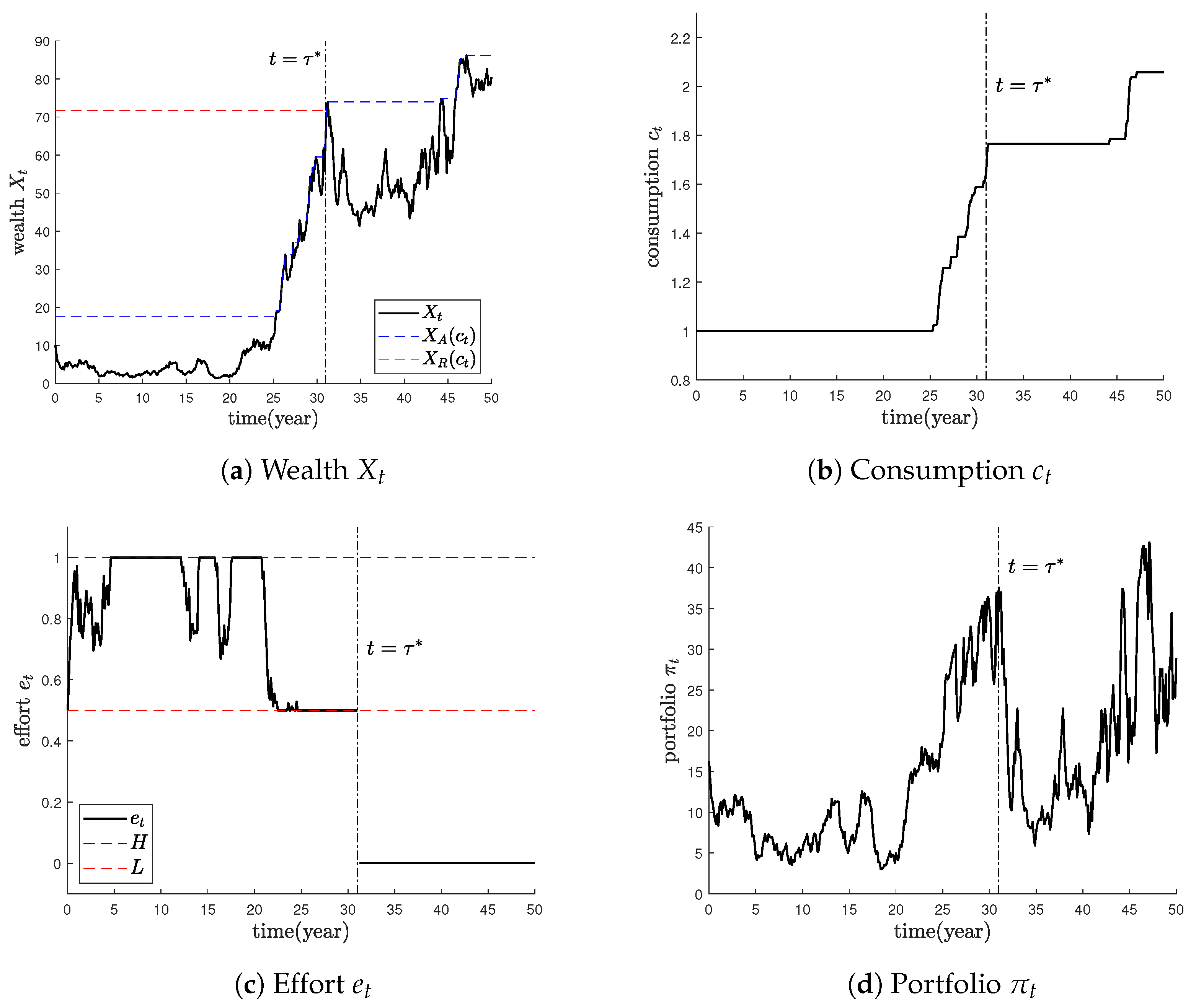
Figure 4 provides simulation results for the optimal strategies. As mentioned earlier, the agent increases consumption whenever their wealth reaches the boundary $X_A\left(c_t\right)$, and chooses early retirement upon reaching $X_R\left(c_t\right)$.

Figure 4. Simulation paths for optimal strategies.

6. Conclusions

In this paper, we have developed a theoretical framework for optimal consumption, investment, retirement, and effort decisions under a consumption ratcheting constraint using a dual-martingale approach within a continuous-time financial market. Our results provide a rigorous mathematical characterization of a single agent’s decision-making process, highlighting the interplay between stochastic control, singular control, and optimal stopping.

While our focus has been on single-agent optimization, we acknowledge that extending this framework to incorporate interactions among heterogeneous agents or emergent phenomena, as typically explored in agent-based modeling (ABM), could offer additional insights. ABM approaches, which simulate the behavior of multiple agents with diverse preferences and strategies, could complement our model by investigating how individual decisions are influenced by collective dynamics. However, since such an extension lies beyond the scope of the current study, and would require significant modifications to the present setup, we leave this for future research.