On Deadlock Analysis and Characterization of Labeled Petri Nets with Undistinguishable and Unobservable Transitions

Abstract

This work addresses the analysis and characterization of deadlocks in discrete-event systems modeled by labeled Petri nets (LPNs) with undistinguishable and unobservable transitions. To provide a solution for the notorious problem, it is essential to present an effective characterization in such a way that deadlock control and synthesis are technically and methodologically possible. To this end, we introduce the notion of dangerous implicit vectors (DIVs), which implicitly threaten the system deadlock-freedom. The set of dead markings is divided into two subsets: dead basis markings (DBMs) and dangerous implicit markings (DIMs). An algorithm is designed to compute the sets of DIVs and DIMs at a given basis state of a system. Moreover, by virtue of linear algebraic equations, we formulate sufficient conditions for identifying the existence of blocking markings in an LPN. Finally, an algorithm is developed to construct an observed graph that is a compendious presentation of the reachability graph of a net system, with respect to the existence of dead reaches. At the end of this paper, experiment results that illustrate the correctness and effectiveness of the reported solution are presented.

1. Introduction

Nowadays, the use of artificial dynamical systems is remarkably increasing in view of the enormous evolution of computer technology. The most important characteristic of these systems is determined by the occurrences of asynchronous events in such a way that they are naturally and soundly labeled as discrete-event systems (DESs) [1]. In fact, many contemporary cyber–physical systems can be investigated from the view of discrete-event systems where the procedure of system analysis and synthesis greatly depends on mathematical system models [2]. Without such a mathematical model, it would be impossible to analyze and control the behavior of a system. Different models are used to achieve this goal, such as Petri nets, automata, Markov chains, etc. However, building on the distinct elements, i.e., places and transitions, that characterize physical system features, Petri nets are a typical modeling paradigm of DESs through the usage of linear algebra and engineering optimization techniques. Nevertheless, several fundamental problems remain open. Among them, we, in this research, focus on the deadlock problem, which is an important issue in designing automated systems [3] and has received much attention from the community of computer science and systems control engineers [4,5,6].

Researchers and practitioners have developed an array of deadlock resolution methods such as those in an early work in [7], where a forbidden state avoidance issue is addressed for a system with unobservable transitions, which is modeled with Petri nets with a known initial marking. The approach is liable to be reshaped for deadlock control. In [8,9], Li and Wonham seminally explore the state-feedback mechanism for the supervisory control of DESs in which certain states are not observable, and a plant is modeled with a finite state automaton in which an event can be controllable (observable) or uncontrollable (unobservable). Their goal is to find necessary and sufficient conditions for the existence of “optimal” state feedback control laws, given a control specification is represented by a finite state automaton.

Proposed in [10] is a deadlock characterization and a control procedure based on an observer of a plant, which is actually what an external agent can observe, representing the system output from the lens of outside observation. By virtue of the characterization, a systematic procedure is presented for deadlock recovery, i.e., a deadlock state can be guided/recovered to a predefined normal state. The main contribution is that the observer, the controller, and the deadlock recovery algorithm are all based on the same linear algebraic techniques. Later, Giua and Seatzu [11] use generalized mutual exclusion constraints, based on the previously mentioned characterization, to ensure the control objective, where a plant is modeled with a Petri net and a generalized mutual exclusion constraint serves as the control specification. They explore a recovery procedure and present a deadlock recovery algorithm using linear algebraic techniques. In these studies, and contrary to the supervisory control theory in the Ramadge–Wonham framework [12], all transitions are, in general, assumed to be controllable and observable, and ordinary Petri nets are usually used to model systems. Partially to this end, but not limited to it, the methodologies of deadlock analysis and control derived from Petri nets are not as general as those from the Ramadge–Wonham paradigm [13,14].

In the literature, people have followed three main lines to deal with the problem of deadlocks in the DESs modeled with Petri nets. First, we mention the deadlock prevention principle [15,16,17,18,19,20], which is an offline computation procedure that imposes restrictions on system evolution to prevent the reachability of dead markings. The prevention is ensured by forbidding all first-met bad markings (FBMs) that represent the first entry from the live zone to the dead zone, which are the partition of the reachability graph of a plant, where the initial state assumed to be legal belongs to the live zone.

Contrary to the deadlock prevention principle, deadlock avoidance [21,22,23,24,25,26] is an online mechanism used to handle the blocking problem in Petri nets. As the mechanism proceeds online, a proper decision is made at each state and issued to the actuators among all possible evolutions with the aim of avoiding deadlocks and keeping the system from being trapped in a deadlock state. However, similar to the previously mentioned methods, deadlock avoidance uses the notions of live zone and deadlock zone to achieve this purpose. Although it generally leads to higher resource utilization and throughput, overly aggressive policies are still not able to totally eliminate all deadlocks in some cases. Then, the necessity to use deadlock recovery strategies naturally comes to mind. Note that a recovery scheme is usually used in a scenario where deadlocks do not cause serious consequences.

To summarize, overly cautious or non-aggressive policies may remove unsafe/illegal states and deadlocks from a closed-loop system, along with certain legal states in a general case. Finally, we briefly explain deadlock detection and recovery techniques [27,28,29,30]. The difference between this mechanism and the two aforementioned methodologies is that a deadlock detection and recovery approach permits the occurrence of a deadlock. Once it occurs, it is detected, and then a recovery policy is initialized to guide and navigate the system to a predefined deadlock-free state by simply reallocating the resources held by the system processes. The efficiency and efficacy of this type of strategy depend upon the response time of the implemented algorithms [31]. A long-term running of a system may provide a large amount of data in such a way that different recovery policies can be well developed offline. Once a deadlock is detected, we may easily propose which type of recovery policy to be applied.

To summarize, the deadlock problem has often been discussed in the literature, and several original theoretical approaches have been proposed [10,11,32,33,34] to solve it. While the previous works usually use ordinary Petri nets to model a system where all transitions are observable (the occurrence of any transition can be detected) and distinguishable (different transitions carry different labels), we deal, in this paper, with the issue of deadlock analysis and control in labeled Petri nets where transitions can be unobservable and undistinguishable. Labeled Petri nets are an important framework of discrete-event systems and their liveness or deadlock-freedom is usually a prerequisite for many problems such as fault diagnosis, opacity verification and enforcement, and state estimation [35]. In fact, as a dominant mathematical tool in discrete-event systems, labeled Petri nets’ liveness analysis and decision have been open issues in the discrete-event system community. Due to its complexity, not enough attention is paid to it and the related results are limited. We are motivated by the importance of deadlock characterization, analysis, and control of a discrete-event system for ensuring the correct and safe functioning of large complex systems. More significantly, the importance of defining the deadlock problem optimally will consequently lead to finding an optimal solution to guarantee the deadlock-freeness of the studied system. Moreover, given the lack of work treating this problem in labeled Petri nets, our contributions come naturally.

This paper will be divided into eight main sections. Section 2 provides a brief introduction to labeled Petri nets as well as a few critical notions. Section 3 introduces the basis reachability graph of a labeled Petri net. In Section 4, we focus on deadlock analysis using reachability graphs and basis reachability graphs. Section 5 elaborates upon dangerous implicit reaches, dangerous implicit markings, and dangerous implicit vectors, which play an important role in deadlock analysis. The main results are presented in this section. A structure called an observed graph for deadlock characterization of labeled Petri nets is deferred to Section 6, where an algorithm is developed for its computation. Experiment results are utilized to illustrate the proposed method in Section 7. Finally, Section 8 concludes the paper, with future topics presented.

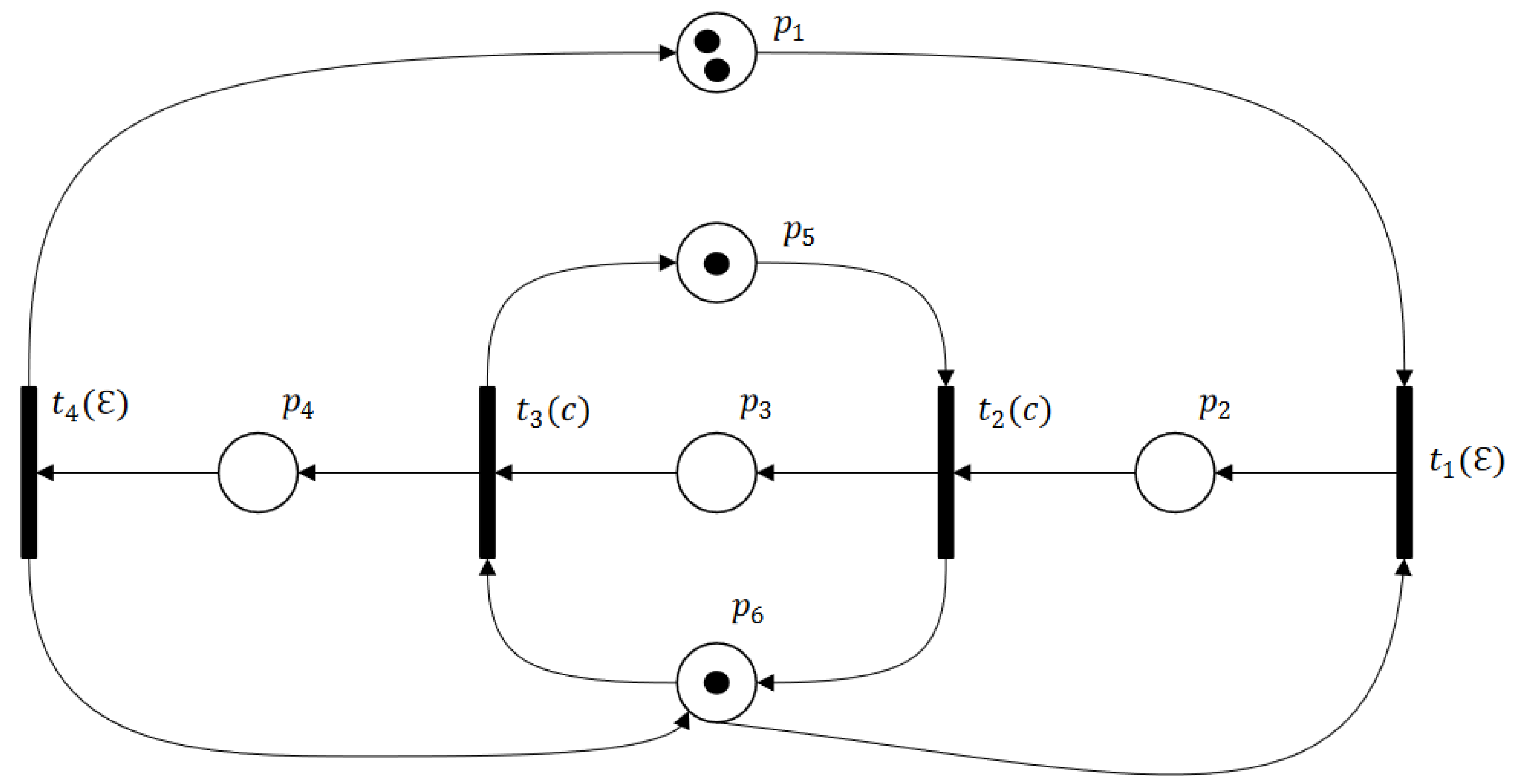
2. Labeled Petri Nets

Petri nets [36] are employed to model a DES of interest. As seen in [37], the reachability graph of a bounded net system is actually a finite state automaton, a deterministic finite automaton as a matter of fact, suggesting that Petri nets and finite state automata are tied up with each other. The preliminaries of finite state automata, Petri nets, and labeled Petri nets are referred to [37].

From the viewpoint of graph theory, a Petri net, simply called a net, is a bipartite digraph that consists of two types of nodes called places and transitions that are usually portrayed by circles and boxes, respectively. Places and transitions are connected by edges, called arcs. In general, the sets of places and transitions in a net are denoted by P and T, respectively. The arcs from places to transition and from transitions to places can be algebraically represented by two functions Pre and Post, respectively. As the sets P and T are finite, Pre and Post can be written as matrices indexed by P and T for computational convenience. Then, a Petri net or net structure can be described as a quadruple $N=(P,T,\mathrm{Pre},\mathrm{Post})$. Tokens in a place signify that particular conditions the place represents hold. A marking of a net is a mapping from the place set P to the set of natural numbers $\mathbb{N}=\{0,1,2,\dots \}$, which is formally defined as $M:P\to \mathbb{N}$. A marking M of a net N indicates the token distribution over its places. Tokens can flow among the places via transitions by following the transition-enabling and firing rules, defining the dynamics of a net system that is symbolized by $(N,M_0)$, where $M_0$ is called the initial marking. That is, a net system can be given by $(N,M_0)$ with $N=(P,T,\mathrm{Pre},\mathrm{Post})$ being a net structure.

With $T^{*}$ being the Kleene closure of transition set T, we usually use $\sigma \in T^{*}$ to denote a transition sequence. From a marking M (not necessarily $M_0$), if a transition sequence $\sigma$ is feasible, write $M[\sigma ⟩M^{\prime }$, where $M^{\prime }$ is said to be the reachable marking from M via $\sigma$. Note that a transition sequence is feasible if the transitions in it can fire sequentially. All the markings reachable from the initial markings via feasible transition sequences form a set called the reachability set, defined as $R(N,M_0)=\{M\in {\mathbb{N}}^{\left|P\right|}\mid \exists \sigma \in T^{*}:M_0[\sigma ⟩M\}$. Keeping the reachability set in mind along with the reachability relation among markings, a digraph called the reachability graph of $(N,M_0)$, denoted as $G(N,M_0)$, can be constructed, where a node is a marking in $R(N,M_0)$ and there is an edge from M to $M^{\prime }$ labeled with $t\in T$ if $M[t⟩M^{\prime }$ holds.

A labeled Petri net (LPN) [38], extended from the Petri net presented above by adjoining two tuples, namely E and ℓ, is a quadruple $G=(N,M_0,E,\ell )$, where

• E is the alphabet, collecting event labels;
• $⟨N,M_0⟩$ is a Petri net system;
• $\ell :T\to E\cup \left\{ϵ\right\}$ is the labeling function such that a transition $t\in T$ is assigned either a label in E or the empty string $\epsilon$.

Note that the labeling function can be, in a usual way, extended as being $\ell :T^{*}\to E^{*}$, i.e., a transition sequence is mapped as a sequence of labels with $\ell \left(\epsilon \right)=\epsilon$. If an event is given a label, its occurrence can be detected by observing the label. Then we group the transitions with labels as $T_o$ and those with the empty string $\epsilon$ as $T_{uo}$, called observable and unobservable transitions, respectively. A major difference between a Petri net and a labeled Petri net lies in the modeling of unobservable transitions in the latter, which stems from the fact that in a real system, sensors are not deployed for all the events, partially due to technical or financial reasons. In other words, if an event is not associated with a sensor, we cannot observe its occurrence, i.e., it is treated as being unobservable. An example of an LPN is shown in Figure 1, where $P=\{p_1,p_2,p_3,p_4,p_5,p_6\}$ is the set of places and $T=\{t_1,t_2,t_3,t_4\}$ is the set of transitions with $\Sigma =\left\{c\right\}$, $T_o=\{t_2,t_3\}$, $T_{uo}=\{t_1,t_4\}$, $\ell \left(t_1\right)=\ell \left(t_4\right)=\epsilon$, and $\ell \left(t_2\right)=\ell \left(t_3\right)=c$.

Figure 1. A labeled Petri net.

Given an LPN $G=(N,M_0,E,\ell )$ and a marking $M\in R(N,M_0)$, the language generated by G from M is defined as

$$\mathcal{L}(G,M)=\{\omega \in E^{*}\mid \exists \sigma \in T^{*}:M[\sigma ⟩\mathrm{and}\ell \left(\sigma \right)=\omega \}.$$

(1)

Furthermore, given a set of markings $Y\subseteq R(N,M_0)$ of G, we define the language generated from the markings in Y as

$$\mathcal{L}(G,Y)=\bigcup _{M\in Y}\mathcal{L}(G,M).$$

(2)

A string belonging to $\mathcal{L}(G,M_0)$ is called an observation. Let $\omega$ be an observation of an LPN $G=⟨N,M_0,E,\ell ⟩$. We define

$$\mathcal{C}\left(\omega \right)=\{M\in {\mathbb{N}}^m\mid \exists \sigma \in T^{*}:M_0[\sigma ⟩M\mathrm{and}\ell \left(\sigma \right)=\omega \}.$$

(3)

as the set of markings consistent with $\omega$. We also define the set of markings generating $\omega$ as

$$\mathcal{I}\left(\omega \right)=\{M\in R(N,M_0)\mid \exists \sigma \in T^{*},\exists M^{\prime }\in R(N,M_0):M[\sigma ⟩M^{\prime }\mathrm{and}\ell \left(\sigma \right)=\omega \}.$$

(4)

By definition, once the word (string) $\omega$ is observed, the sets $\mathcal{C}\left(\omega \right)$ and $\mathcal{I}\left(\omega \right)$ are non-empty sets. Given an observation $\omega \in \mathcal{L}(G,M_0)$, ${\omega }^{\prime }$ is a prefix of $\omega$ if and only if there exists a string $\nu \in E^{*}$ such that $\omega ={\omega }^{\prime }\nu$. We write $\overline{\omega }$ to denote the prefix set of $\omega$ with $\epsilon \in \overline{\omega }$ and $\omega \in \overline{\omega }$. For a set of observations $L\subseteq \mathcal{L}(G,M_0)$, we define the prefix-closure of L as $\overline{L}=\{\nu \in \mathcal{L}(G,M_0)\mid \exists \omega \in L:\nu \in \overline{\omega }\}$. Simply put, $\overline{L}$ consists of all the prefixes of all the strings in L. It is trivial that $\epsilon \in \overline{L}$ and for any string $\omega \in L$, $\omega \in \overline{L}$ if L is not empty.

3. Minimal Explanation and Basis Reachability Graph

The concept of a basis reachability graph is proposed in [39,40], which serves as a compact way to represent the reachability set of an LPN to solve fault diagnosis and many other problems in the context of discrete-event systems. It has been used to address the issues related to observability, e.g., diagnosability and opacity verification and enforcement problems [39,40,41]. A generalization of the basis reachability graph is proposed by Ma and his colleagues in [42], where a more fundamental structure that only contains basis markings independently from the system’s partition is defined. In this section, we will provide some basic definitions that will be used in the following.

3.1. Minimal Explanation and Minimal E-Vector

Definition 1 

(Basis Partition [42]). Given a net $N=(P,T,Pre,Post)$ with $T=T_E\cup T_I$ and $T_E\cap T_I=\varnothing$, a pair $\pi =(T_E,T_I)$ is called a basis transition partition of the transition set T if the $T_I$-induced subnet is acyclic.

The transitions in $T_E$ (resp. $T_I$) are said to be explicit (resp. implicit). Write $|T_E|=n_E$ and $|T_I|=n_I$. In our research, unobservable transitions in a labeled Petri net will be collected in set $T_I$. The assumption that in the $T_I$-induced subnet, there is no cycle ensures that an observable event can be observed within a finite time; otherwise, a system may be infinitely cycled without any observational output. Given a Petri net $N=(P,T,Pre,Post)$, a basis partition $\pi =(T_E,T_I)$, a marking M, and a transition $t\in T_E$, we define the set of explanations of transition t at marking M as

$$\Sigma (M,t)=\{\sigma \in T_I^{*}\mid M[\sigma ⟩M^{\prime }\mathrm{and}{M}^{\prime }\ge Pre(·,t)\}.$$

(5)

The set of e-vectors (explanation vectors), which collects the firing vectors associated with the firing sequences in $\Sigma (M,t)$, is defined as

$$Y(M,t)=\{y_{\sigma }\in {\mathbb{N}}^{n_I}\mid \sigma \in \Sigma (M,t)\}.$$

(6)

We also define the set of minimal explanations of transition $t\in T_E$ at marking M as

$${\Sigma }_{\min }(M,t)=\{\sigma \in \Sigma (M,t)\mid \nexists {\sigma }^{\prime }\in \Sigma (M,t):y_{{\sigma }^{\prime }}⪇y_{\sigma }\}.$$

(7)

The corresponding set of minimal explanation vectors is

$$Y_{\min }(M,t)=\{y_{\sigma }\in {\mathbb{N}}^{n_I}\mid \sigma \in {\Sigma }_{\min }(M,t)\}$$

(8)

Given a marking M and an explicit transition $t\in T_E$, the work in [39] proposes an efficient algorithm to compute the set of minimal e-vectors $Y_{\min }(M,t)$.

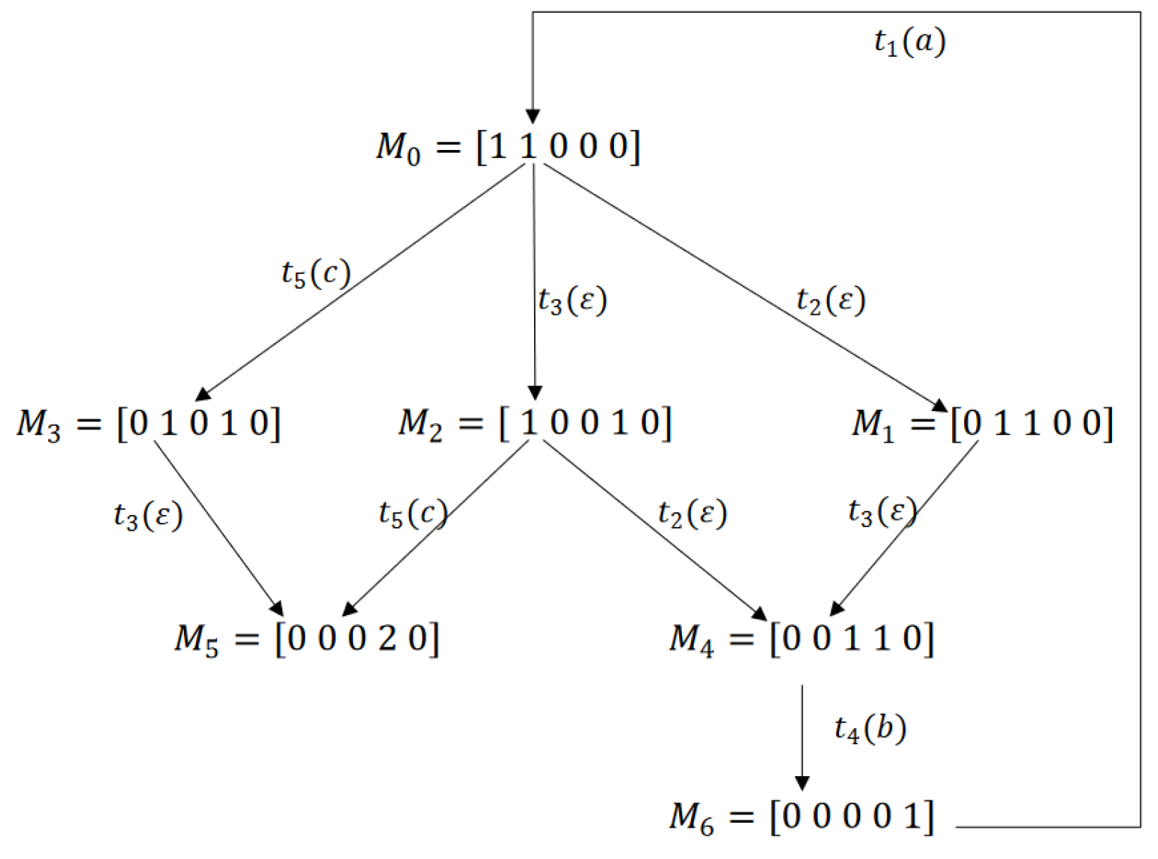
3.2. Basis Reachability Graph

Definition 2 

(Basis Marking [42]). Given a Petri net $N=(P,T,\mathit{Pre},\mathit{Post})$ with an initial marking $M_0$ and a basis partition $\pi =(T_E,T_I)$, its basis marking set $\mathcal{M}(N,M_0,\pi )$ is defined as follows:

• $M_0\in \mathcal{M}(N,M_0,\pi )$;
• If $M\in \mathcal{M}(N,M_0,\pi )$, then the predicate holds: $\forall y\in Y_{\mathit{min}}(M,t):(M^{\prime }=M+{\mathcal{C}}_I·y+\mathcal{C}(·,t))\Rightarrow (M^{\prime }\in \mathcal{M}(N,M_0,\pi ))$

where ${\mathcal{C}}_I$ is the incidence matrix of N restricted to the transition set $T_I$. A marking M in $\mathcal{M}(N,M_0,\pi )$ is called a basis marking of $⟨N,M_0⟩$ with respect to $\pi =(T_E,T_I)$.

Definition 3 

(Basis Reachability Graph [42]). Given a bounded net $N=(P,T,\mathit{Pre},\mathit{Post})$ with an initial marking $M_0$ and a basis partition $\pi =(T_E,T_I)$, its basis reachability graph (BRG) is a non-deterministic finite state automaton, represented by a quadruple $\mathcal{B}=(\mathcal{M},T_r,\Delta ,M_0)$ such that

• the state set $\mathcal{M}$ is the set of basis markings;
• the event set $T_r$ is the set of pairs $(t,y)\in T_E\times {\mathbb{N}}^{n_I}$;
• the transition relation Δ is

  $$\Delta =\{(M_1,(t,y),M_2)\mid t\in T_E,y\in Y_{\min }(M_1,t),\mathrm{and}{M}_2=M_1+\mathcal{C}·y+\mathcal{C}(·,t)\}$$
• the initial state is the initial marking $M_0$.

An algorithm is proposed in [42] that iteratively computes basis markings and constructs a BRG. We use $\mathcal{B}(N,M_0,\pi )$ to denote the BRG of a net $⟨N,M_0⟩$ with basis partition $\pi$. If no confusion arises, it is simply written as $\mathcal{B}$.

This algorithm computes the set of all minimal explanations of each selected marking M and associates each explanation $y\in Y_{\min }(M,t)$ with a new marking $M^{\prime }$ defined by the state equation of a basis marking $M^{\prime }=M+{\mathcal{C}}_I·y+\mathcal{C}(·,t)$. Each new marking is defined as an unchecked marking, and this procedure runs iteratively until there are no unchecked markings. For a bounded Petri net, based on $\mathcal{M}\subseteq R(N,M_0)$, such an algorithm can terminate in a finite amount of time.

Given a labeled Petri net (not associated with a real system), $(T_E,T_I)$ is a purely theoretical partition that can be arbitrary: Different partitions lead to different BRGs with different sizes. In particular, if $T_I=\varnothing$, the BRG under the partition $(T,\varnothing )$ is exactly the reachability graph of a net system. BRG-based methods are extensively developed for addressing multiple problems in DESs, e.g., opacity verification and enforcement, fault diagnosis and diagnosability analysis, fault predictability, and supervisory control, where the unobservable transitions are collected into $T_I$ for the construction of a BRG.

In a general case, the size of a BRG of a net system is (much) smaller than its reachability graph. Suppose that in a reachability graph, there are k paths from a marking M to markings $M_1$, $M_2$, …, $M_k$ through unobservable transition sequences ${\sigma }_{u1}$, ${\sigma }_{u2}$, $\dots ,{\sigma }_{uk}$, respectively, i.e., $M[{\sigma }_{ui}⟩M_i$, for all $i\in \{1,2,\dots ,k\}$, and there exists an explicit transition $t\in T_E$ that is enabled at $M_i$ for all $i\in \{1,2,\dots ,k\}$. Then in its corresponding BRG, only one path is kept, whose associated unobservable transition sequence has a minimal explanation vector. Other paths can be removed from the reachability graph, which does not affect the observational behavior. This is why BRGs are, in general, small-sized, such that they find their extensive applications in many problems in the DES community, such as opacity verification and enforcement, fault diagnosis, diagnosability analysis and enforcement, supervisory control, and so on. Note that it has been interesting to apply the idea of BRGs to the automata such that a reduced model may be obtained. Experimental studies show that with the increase of net system size, the effect of using BRGs instead of reachability graphs would become much more obvious and beneficial in computation [42].

4. Deadlock Analysis

In this section, we will give a brief overview of reachability graph-based methodologies dealing with the deadlock problem in a DES modeled with Petri nets. In fact, when treating the problem, we can distinguish between structure and reachability graph analysis. In this paper, we are interested in the latter, providing effective solutions for the deadlock problem for an LPN.

4.1. Analysis of Reachability Graph

The authors of [43] split a reachability graph of a net model into two zones: a deadlock zone (DZ) and a live zone (LZ). The DZ is composed of deadlock states (or called deadlock markings), at which no transition is defined or feasible, and partial deadlock states, which are deadlock-reachable but not co-reachable with respect to the initial marking—from which the initial marking cannot be reached but a deadlock can be reached. Then, LZ contains all the markings in the reachability set, which do not belong to the DZ. In other words, a marking (state) in LZ is reachable and co-reachable with respect to the initial marking. Suppose that all the transitions in a system model are controllable. A control policy is maximally permissive if the closed-loop system keeps all the states/markings in its LZ [44].

Sometimes, we also use $LZ$ ($DZ$) to stand for the set of elements in LZ (DZ). Note that in [45], a state/marking M in LZ is said to be dangerous if its one-step extension falls into the DZ, i.e., there exist a transition $t\in T$ and a marking $M^{\prime }$ such that $M[t⟩M^{\prime }$ and $M^{\prime }\in DZ$ holds. In this case, the pair $(M,t)$ is called a marking/transition separation instance. If a monitor can be designed for each marking/transition separation instance such that all the states in the LZ are kept in the closed-loop system and all the states in the DZ are removed, then we say that the policy derived from the set of monitors is the least restrictive or maximally permissive. In Figure 2, we show the partition of the reachability graph of some LPN, where $\{t_1,t_4,t_5,t_6,t_8\}$ is the set of observable transitions.

Figure 2. Partitioned reachability graph of an LPN.

However, the computation of a reachability graph is usually expensive, as the state space of a system modeled with a Petri net grows exponentially with the system scale, i.e., the place set and the initial marking. Given a real system, a complete enumeration of reachable is, in general, infeasible. This is why we have to explore other computationally efficient methods to address the related problems in DESs, leading to the birth of BRGs. As seen after the proposal of BRG, there is a deluge of methods for the various problems in DESs using Petri nets. In this paper, we try to employ this notion to address the deadlock characterization and analysis of a DES, which is partially observed, using labeled Petri nets.

4.2. Analysis of Basis Reachability Graph

Under the assumption that the $T_{uo}$-induced subnet is acyclic, the study in [39,40] uses the original BRG to solve the fault diagnosis problem. A generalization of BRG has been introduced later in [42]. This particular graph preserves the necessary information on marking reachability but is much smaller in practice application systems so that the notorious state explosion problem is, to some extent, mitigated. In this subsection, we focus on analyzing deadlocks based on BRGs and studying their effectiveness in characterizing deadlocks in systems modeled by LPN.

Definition 4 

([42]). Given a net $N=(P,T,\mathit{Pre},\mathit{Post})$, a basis partition $\pi =(T_E,T_I)$, and a basis marking $M_b\in \mathcal{M}$, the implicit reach of $M_b$, denoted by $R_I\left(M_b\right)$, is defined as

$$R_I\left(M_b\right)=\{M\in {\mathbb{N}}^m\mid \exists \sigma \in T_I^{*}:M=M_b+\mathcal{C}·y_{\sigma }\}.$$

(9)

By definition, the implicit reach of a basis marking $M_b$ is the set of markings reachable from $M_b$ by firing only implicit transitions.

Corollary 1 

([42]). Given a Petri net $⟨N,M_0⟩$ and its BRG $\mathcal{B}$, the following holds

$$R(N,M_0)=\bigcup _{M_b\in \mathcal{M}}{R}_I\left(M_b\right).$$

(10)

As Corollary 1 shows, we can easily observe that the implicit reaches of all basis markings span exactly the state space of a net system. The main contribution of a BRG is that it prevents the exhaustive exploration of all reachable states. As only the minimal e-vector is taken into account for each basis marking and observable transition when constructing a BRG, some edges in a reachability graph are not explicitly represented in a BRG so that its size is significantly reduced, particularly if the set of implicit transitions is large. However, this may ignore useful information about deadlock markings. Note that, for fault diagnosis and diagnosability analysis, under the assumption that a plant is live, a BRG does not lose any useful information. However, as suggested by the liveness assumption, the aforementioned BRG is problematic for deadlock analysis of a labeled Petri net. We now touch upon some definitions that are essential and critical to formalize and develop the main results in this paper.

Definition 5. 

Given a marking M and an explicit transition $t\in T_E$, the set of entire explanations at M is defined as

$$\mathcal{E}\left(M\right)=\bigcup _{t\in T_E}\Sigma (M,t).$$

(11)

We also define the set of entire explanation vectors as

$$Y_T\left(M\right)=\bigcup _{t\in T_E}Y(M,t).$$

(12)

Similarly, we introduce the set of entire minimal explanations at M as

$${\mathcal{E}}_{\mathit{min}}\left(M\right)=\bigcup _{t\in T_E}{\Sigma }_{\mathit{min}}(M,t).$$

(13)

and its corresponding set of entire minimal e-vectors as

$$Y_{T_{\mathit{min}}}\left(M\right)=\bigcup _{t\in T_E}{Y}_{\mathit{min}}(M,t).$$

(14)

In other words, $\mathcal{E}\left(M\right)$ represents the set of all implicit sequences whose firing at the marking M enables an explicit transition $t\in T_E$, while ${\mathcal{E}}_{\min }\left(M\right)$ is the set of all minimal implicit sequences feasible at $M_b$, at which an explicit transition $t\in T_E$ is enabled. The number of arcs in a BRG, where $M_b$ is the input vertices, is equal to the cardinality of ${\mathcal{E}}_{\min }\left(M_b\right)$.

Lemma 1. 

Given an LPN $G=(N,M_0,E,\ell )$, a basis partition $\pi =(T_E,T_I)$, and an explicit transition $t_E\in T_E$, a basis marking $M_b$ is reachable from another basis marking if it satisfies

$$M_b=\sum _{i=1}^n{\alpha }_i{M}_{b_i}+{\mathcal{C}}_I·y_I+\mathcal{C}(·,t_E)$$

(15)

with $y_1\in Y_{\mathit{min}}(M_b,t_E)$, ${\sum }_{i=1}^n{\alpha }_i=1$, and ${\alpha }_i\in \{0,1\}$.

Proof. 

This result stems from the state equation of a basis marking. By ${\alpha }_i\in \{0,1\}$ and ${\sum }_{i=1}^n{\alpha }_i=1$, we have one and only one ${\alpha }_i=1$ for some i. In other words, we have at least one basis marking $M_{b_i}$ such that

$$M^{\prime }=M_{b_i}+{\mathcal{C}}_I·y_I+\mathcal{C}(·,t_E).$$

(16)

Based on the state equation of a basis marking, if $M\in \mathcal{M}(N,M_0,\pi )$, then for all $t\in T_E$ and for all $y\in Y_{\min }(M,t)$, we have

$$M^{\prime }=M+{\mathcal{C}}_I·y+\mathcal{C}(·,t)\Rightarrow M^{\prime }\in \mathcal{M}(N,M_0,\pi ).$$

(17)

Thus, we conclude that $M^{\prime }$ is a reachable basis marking.    □

As indicated by the lemma, a marking M is a reachable basis marking if there exists, at least, another reachable basis marking from which M can be reachable by firing a minimal explanation followed by its corresponding explicit transition $t_E$.

Definition 6. 

Given an LPN $G=(N,M_0,E,\ell )$, a basis partition $\pi =(T_E,T_I)$, and an explicit transition $t_E\in T_E$, a marking M is a dead basis marking (DBM) if it satisfies the following linear system:

$$DBM\left(M_b\right):=\left\{\begin{array}{cccc}\hfill M_b& =\sum _{i=1}^n{\alpha }_i{M}_{b_i}+{\mathcal{C}}_I·y_I+\mathcal{C}(·,t_E)\hfill & \hfill & \left(a\right)\hfill \\ \hfill \mathcal{E}\left(M_b\right)& =\varnothing \hfill & \hfill & \left(b\right)\hfill \\ \hfill \sum _{i=1}^n{\alpha }_i& =1\hfill & \hfill & \left(c\right)\hfill \\ \hfill {\alpha }_i& \in \{0,1\}\hfill & \hfill & \left(d\right)\hfill \\ \hfill y_1& \in Y_{\min }(M_b,t_E)\hfill & \hfill & \left(e\right)\hfill \end{array}\right.$$

(18)

In other words, a marking M is said to be a DBM if there exists a basis marking $M_{b_i}$, from which it is reachable by firing $\sigma ={\sigma }_I{t}_E$ with ${\sigma }_I$ a minimal explanation of $t_E$, and there does not exist any implicit sequence feasible at $M_b$ that can enable an explicit transition. Note that, despite the set of entire explanations at $M_b$ is empty, the set of implicit reaches $R_I\left(M_b\right)$ could not be so. From Definition 10, we derive the following sufficient condition for deadlock existence in an LPN.

Theorem 1. 

(Sufficient Condition) Given an LPN $G=(N,M_0,E,\ell )$, a basis partition $\pi =(T_E,T_I)$, a DBM $M_b$, and a marking $M^{\prime }\in {\mathbb{N}}^m$, the following predicate holds:

$$M^{\prime }\in R_I\left(M_b\right)\Rightarrow M^{\prime }\in DZ$$

(19)

Proof. 

The fact that $M_b$ is a DBM implies $\mathcal{E}\left(M_b\right)=\varnothing$. We have $R(N,M_b)=R_I\left(M_b\right)$, and for all $M^{\prime }\in R_I\left(M_b\right)$ such that $M_0[\sigma ⟩M^{\prime }$, it holds $\sigma \notin \mathcal{E}\left(M_b\right)$, leading to the truth of $M^{\prime }\in DZ$.    □

Proposition 1. 

Given an LPN $G=(N,M_0,E,\ell )$, a basis partition $\pi =(T_E,T_I)$, and a marking M, if M is a DBM, then $M\in DZ$ holds.

Proof. 

The proof of Proposition 1 derives from Theorem 1. Suppose that M is a dead basis marking. Theorem 1 has shown $R(N,M)=R_I\left(M\right)\subseteq DZ$. We conclude that from M, only the markings in $DZ$ are reachable. Hence, $M\in DZ$ holds.    □

Theorem 1 gives a sufficient condition to make a decision about the safeness of a basis marking’s reaches. In fact, once the set of entire explanations feasible at $M_b$ is empty, we can easily conclude that only implicit transitions can be feasible at $M_b$. This means that the reachability set of the basis marking $M_b$ is equal to its implicit reach. Note that a BRG is founded under the assumption of acyclicity of the $T_I$-induced subnet. Therefore, there does not exist any implicit sequence feasible at $M_b$ that can return the system to its optimal behavior. In this case, any marking $M^{\prime }$ reachable from $M_b$ (with $M^{\prime }\in R_I\left(M_b\right)$) should necessarily be a dead state, a partial deadlock state that necessarily leads to deadlocks.

Example 1. 

Let us consider the LPN in Figure 3, whose transition partition is $\pi =(T_I,T_E)$ with $T_E=\{t_1,t_4,t_5\}$ and $T_I=\{t_2,t_3\}$. The initial marking is $M_0=p_1+p_2$. As shown in Figure 4, the reachability graph contains seven markings, from which we can easily extract the deadlock zone $DZ=\{M_3,M_5\}$. The BRG of this example is visualized in Figure 5. The basis marking $M_{b2}$ is a DBM since it is reachable from $M_{b0}$ by firing $(t_5,y)$, where $y=[0,0]$ and $\mathcal{E}\left(M_{b2}\right)=\varnothing$. Consider the implicit reach of $M_{b2}$, $R_I\left(M_{b2}\right)=\left\{M_5\right\}\subseteq DZ$ holds. By Proposition 1, we have $M_{b2}\in DZ$.

Figure 3. A labeled Petri net.

Figure 4. Reachability graph of the LPN in Figure 3.

Figure 5. The BRG of the LPN in Figure 3.

Although the DMBs of an LPN are covered by its BRG, it is not able to fully characterize the deadlock problem in the LPN. In fact, the basis reachability graph covers only deadlock states reachable by firing minimal explanations, neglecting thus other feasible implicit events that may threaten the system’s safeness and lead to deadlocks. To clearly explain this point, let us introduce Example 2, which illustrates the weakness of a BRG in deadlock recognition.

Example 2. 

Consider the Petri net in Figure 1 with an initial marking $M_0$, where $M_0\left(p_1\right)=2$, $M_0\left(p_5\right)=M_0\left(p_6\right)=1$, and $M_0\left(p\right)=0$ for other places. The set of transitions T is divided into $T_0=\{t_2,t_3\}$ and $T_{uo}=\{t_1,t_4\}$.

The reachability graph of the net model, shown in Figure 6, has five reachable markings. The firing of $t_1$ from the marking $M_2$ leads the system to a dead marking $M_4$. While considering a basis partition $\pi =(T_E,T_I)$ with $T_E=T_0$ and $T_I=T_{uo}$, Figure 7 defines its BRG. As shown in the figure, this graph is composed of three basis markings. Regarding deadlocks, it gives $DZ=\left\{M_4\right\}$. However, since this dead state is not reachable by firing a minimal explanation, the BRG of this example does not contain any DBM, and the sequence of transitions leading the system to the deadlock zone is not taken into account by the BRG. Thus, the weakness of a BRG facing this type of deadlock clearly appears. Note that the cycle in Figure 7 is due to the unobservability of transitions $t_1$ and $t_4$.

Figure 6. RG of the LPN in Figure 1.

Figure 7. BRG of the LPN in Figure 1.

In this section, we have shown that using the original BRG we cannot fully address the deadlock problem. In the next section, we will introduce new concepts that are able to deal with deadlock characterization and analysis of an LPN.

5. Dangerous Implicit Reaches

In this section, we propose new concepts that enable us to identify the existence of deadlocks in systems modeled by an LPN. A system under consideration in this research is supposed to be arbitrarily labeled, i.e., no condition or restriction is imposed on the labeling function $\ell :T^{*}\to E^{*}$. Hence, the system may contain undistinguishable transitions, i.e., at a marking M, two (or more) enabled transitions may share the same label (e.g., a). We denote the set of undistinguishable transitions with respect to a label $\sigma$ as $T_{ud}\left(\sigma \right)=\{t\in T|\ell \left(t\right)=\sigma \in E_{\epsilon }\}$. Moreover, the set of distinguishable transitions in an LPN is denoted by $T_d$. By definition, $T_{uo}\subseteq T_{ud}$ holds, where $T_{ud}={\bigcup }_{\sigma \in E_{\epsilon }}{T}_{ud}\left(\sigma \right)$ is the set of undistinguishable transitions. Hence, the transitions are grouped as $T=T_d\cup T_{udo}\cup T_{uo}$, where $T_{udo}$ is the set of undistinguishable transitions but observable, i.e., $T_{udo}={\bigcup }_{\sigma \in E_{\epsilon }}{T}_{udo}\left(\sigma \right)$, where $T_{udo}\left(\sigma \right)=\{t\in T|\ell \left(t\right)=\sigma \in E\}$.

Consider a system modeled with an LPN and consistent with the aforementioned description. With respect to the concept of basis reachability graph, we can classify the set of implicit reachable states from a basis marking $M_b\in \mathcal{M}$ to three main subsets: minimal explanations, non-minimal explanations, and non-explanation sequences. As we have proven in the previous section, if a deadlock state is reachable by firing an explicit transition preceded by one of its minimal explanations, the BRG can identify such a deadlock state. However, the BRG is still unable to identify deadlocks reachable by firing non-minimal explanations or implicit sequences that can never belong to the set of entire explanations.

5.1. Dangerous Implicit Markings (DIMs) and Dangerous Implicit Vectors (DIVs)

At the beginning of this subsection, let us introduce some results that will be used in the following to minimize the related computations.

Theorem 2. 

Suppose that $\sigma =t_1{t}_2\in T^{*}$ is firable starting from a marking $M_1$ with $M_1[t_1⟩M_2[t_2⟩M_3$ in an PLN. The following holds:

$$\left(M_1[t_1⟩M_2[t_2⟩M_3\right)\wedge (\exists M_4\in {\mathbb{N}}^m:M_1[t_2⟩M_4)\Rightarrow M_4[t_1⟩M_3$$

(20)

Proof. 

Let $\sigma =t_1{t}_2$ and $M_1[t_1⟩M_2[t_2⟩M_3$. This implies that $M_3=M_1+\mathcal{C}(·,t_1)+\mathcal{C}(·,t_2)\ge 0$. Suppose that $t_2$ is firable from $M_1$ with $M_1[t_2⟩M_4$. Then, we have $M_4=M_1+\mathcal{C}(·,t_2)\ge 0$. Hence, we obtain the following system

$$\left\{\begin{array}{c}{M}_1+\mathcal{C}(·,t_1)+\mathcal{C}(·,t_2)\ge 0\hfill \\ M_1+\mathcal{C}(·,t_2)\ge 0\hfill \end{array}\right.$$

(21)

which indicates $M_4+\mathcal{C}(·,t_1)\ge 0$. Accordingly, we conclude that from $M_4$ we necessarily have $M_4[t_1⟩$ and the reachable marking is $M_3$.    □

Corollary 2. 

Given two sequences $\sigma ,{\sigma }^{\prime }\in T^{*}$, where $\sigma =t_1{t}_2\cdots t_n$, $t_i\in \sigma$, and ${\sigma }^{\prime }=\sigma \setminus \left\{t_i\right\}$, suppose that there is a marking $M_1\in {\mathbb{N}}^m$ from which $t_1,t_2,\cdots ,t_n$ are firable sequentially with $M_1[t_1⟩M_2[t_2⟩\cdots [t_n⟩M_n$. If ${\sigma }^{\prime }$ is firable from $M_1$ with $M_1[{\sigma }^{\prime }⟩M_x$, then $M_x[t_i⟩M_n$ holds.

Proof. 

The proof of this corollary derives from Theorem 2. In fact, suppose that from a marking $M\in {\mathbb{N}}^m$ we have $M[\sigma ⟩M^{\prime }$. This implies that (1) $M+C_y\ge 0$ with $y=\pi \left(\sigma \right)$ and ${\mathcal{C}}_y=\mathcal{C}(·,t_1)+\mathcal{C}(·,t_2)+\cdots +\mathcal{C}(·,t_n)$. If $M[{\sigma }^{\prime }⟩M^{″}$, then (2) $M^{″}=M+\mathcal{C}(·,t_1)+\cdots +\mathcal{C}(·,t_{i-1})+\mathcal{C}(·,t_{i+1})+\cdots +\mathcal{C}(·,t_n)$ and $\mathcal{C}(·,t_{i+1})+\cdots +\mathcal{C}(·,t_n)\ge 0$. By (1) and (2) we conclude $M^{″}+\mathcal{C}(·,t_i)\ge 0$ and $M^{″}+\mathcal{C}(·,t_i)=M^{\prime }$.    □

As a matter of fact, Corollary 2 is a generalization of Theorem 2. In what follows, we touch upon a primary notion called dangerous implicit marking, which is pivotal to the development of this research.

Definition 7. 

Given an LPN $G=(N,M_0,E,\ell )$, a basis marking $M_b$, and a vector $y_I\in {\mathbb{N}}^{n_I}$, let $M_b^{\prime }=M_b+C_I·y_I$ with $y_I\ge 0$ and $\nexists y_I^{\prime }\in Y_T\left(M_b\right)$ such that $y_I^{\prime }\ge y_I$. Then $y_I$ is said to be a dangerous implicit vector (DIV), while $M_b^{\prime }$ is called a dangerous implicit marking (DIM).

Further, we define the set of Dangerous Implicit Vectors (DIVs) at $M_b$ by

$$Y_{\beta }\left(M_b\right)=\{y\in {\mathbb{N}}^{n_I}\mid M_b^{\prime }=M_b+{\mathcal{C}}_I·y_I\ge 0\mathrm{and}(\nexists y_I^{\prime }\in Y_T\left(M_b\right):y_I^{\prime }\ge y_I)\}$$

(22)

Moreover, we define the set of Dangerous Implicit Markings (DIMs) reachable from $M_b$ as

$$M_{\beta }\left(M_b\right)=\{M^{\prime }\in {\mathbb{N}}^m\mid M_b^{\prime }=M_b+{\mathcal{C}}_I·y_I\ge 0\mathrm{and}{y}_I\in Y_{\beta }\left(M_b\right)\}$$

(23)

In other words, consider a basis marking $M_b$ and a vector $y\in {\mathbb{N}}^{n_I}$ feasible at $M_b$. The vector $y_I$ is dangerous because it can never be an explanation vector of any explicit transition at $M_b$, i.e., for any feasible implicit sequence of transition ${\sigma }^{\prime }$ at $M^{\prime }$, where $M^{\prime }=M_b+{\mathcal{C}}_I·y_I$ is the marking reachable by firing $y_I$ from $M_b$, the sequence ${\sigma }^{\prime }{\sigma }_I$ can never belong to the set of entire explanations at $M_b$. In this case, the marking reachable by firing an implicit sequence ${\sigma }_I$ from $M_b$, with $y_I=\pi \left({\sigma }_I\right)$, is called a dangerous implicit marking.

Theorem 3. 

Given an LPN $G=(N,M_0,E,\ell )$, a basis marking $M_b$, and a sequence of implicit transitions ${\sigma }_I$ satisfying:

$$\left\{\begin{array}{c}{M}_b[{\sigma }_I⟩,\hfill \\ {\sigma }_I\notin \overline{\mathcal{E}\left(M_b\right)},\hfill \\ {\sigma }_I\in T_I^{*},\hfill \end{array}\right.$$

(24)

($\overline{\mathcal{E}\left(M_b\right)}$ denotes the prefix-closure of $\mathcal{E}\left(M_b\right)$). let $S=\{M^{\prime }\in {\mathbb{N}}^m\mid M^{\prime }=M_b+{\mathcal{C}}_I·y_I^{\prime }\ge 0,{\sigma }_I^{\prime }\in T_I^{*},y_I^{\prime }=\pi \left({\sigma }_I^{\prime }\right),\mathrm{and}{\sigma }_I^{\prime }\in \overline{{\sigma }_I^{\prime }}\}$ be a set of markings, where $\overline{{\sigma }_I^{\prime }}$ denotes the prefix set of ${\sigma }_I^{\prime }$. ($\overline{{\sigma }_I}$ denotes the prefix set of ${\sigma }_I$). Then, for any $M\in S$, $M\in DZ$.

Proof. 

Let $M_b\in {\mathbb{N}}^m$ be a basis marking and ${\sigma }_I,{\sigma }_I^{\prime }\in T_I^{*}$ be two implicit sequences with ${\sigma }_I\in \overline{{\sigma }_I^{\prime }}$. Suppose that $M_b$ and ${\sigma }_I$ verify Theorem 3. Since ${\sigma }_I\in \overline{{\sigma }_I^{\prime }}$ and ${\sigma }_I\notin \mathcal{E}\left(M_b\right)$, we have ${\sigma }_I^{\prime }\notin \mathcal{E}\left(M_b\right)$. Let us consider now $S=\{M^{\prime }\in {\mathbb{N}}^m\mid M^{\prime }=M_b+{\mathcal{C}}_I·y_I^{\prime }\ge 0\}$. We aim to prove that for all $M^{\prime }\in S$, $M^{\prime }\in DZ$.

(a)

By $M_b[{\sigma }_I⟩$, $M^{\prime }=M_b+{\mathcal{C}}_I·y_I^{\prime }>0$. Moreover, there does not exist $t_E\in T_E$ such that $M^{\prime }[t_E⟩$ due to ${\sigma }_I^{\prime }\notin \mathcal{E}\left(M_b\right)$.

(b)

As is known, the $T_I$-induced subnet is acyclic, implying that the predicate holds: $\nexists {\sigma }_I=t_{I_1},t_{I_2},\dots ,t_{I_k}$: $M_1[t_{I_1}⟩M_2[t_{I_2}⟩\dots M_k[t_{I_k}⟩M_1$. That is to say, from the marking $M^{\prime }$, we cannot co-reach $M_0$ by firing only implicit transitions.

By (a) and (b), we conclude that for all $M^{\prime }\in S$, $M_0\notin R(N,M^{\prime })$ holds.    □

In simple words, consider an LPN $G=(N,M_0,E,\ell )$, an arbitrary basis partition $\pi =(T_E,T_I)$, and a basis marking $M_b$. Under the assumption that the $T_{uo}$-induced subnet is acyclic, we have proven by Theorem 3 that any marking $M^{\prime }$ reached by firing an implicit sequence ${\sigma }_I$ that does not belong to $\overline{\mathcal{E}\left(M_b\right)}$, the prefix-closure of the set of entire explanations $\mathcal{E}\left(M_b\right)$, is either a dead marking or a marking that inevitably leads the system to a blocking state. Thus, $M^{\prime }$ belongs necessarily to the dead zone (DZ).

Proposition 2. 

Given an LPN $G=(N,M_0,E,\ell )$, a basis marking $M_b$, and a dangerous implicit vector $y_I\in Y_{\beta }\left(M_b\right)$ with $M_I^{\prime }=M_b+{\mathcal{C}}_I·y_I$, $M_b^{\prime }$ is a DIM and for all $y_I^{″}\in {\mathbb{N}}^{n_I}$ such that $M_b^{″}=M_b^{\prime }+{\mathcal{C}}_I·y_I^{″}\ge 0$, $M_B^{″}\in DZ$ holds.

Proof. 

Given a basis marking $M_b$ and a sequence of implicit transitions ${\sigma }_I\in T_I^{*}$ firable from $M_B$ with $\pi \left({\sigma }_I\right)=y_I$, suppose that $y_I$ is a DIV, i.e., there does not exist $y_I^{\prime }\in Y_T\left(M_b\right)$ such that $y_I^{\prime }\ge y_I$. Then, for all $y_x\in {\mathbb{N}}^{n_I}$, there does not exist $y_I^{\prime }\in Y_T\left(M_b\right)$ such that $y_I^{\prime }\ge y_I+y_x$. We have for all $\sigma ={\sigma }_I{\sigma }_x$ such that $M_b[\sigma ⟩$, $\sigma \notin \overline{\mathcal{E}\left(M_b\right)}$ is true and thus by Theorem 3, $M_b^{″}=M_b+{\mathcal{C}}_I·y_{\sigma }\in DZ$ holds.    □

By virtue of DIV and DIM notions, Proposition 2 represents a generalization of Theorem 3. In fact, when checking the safeness of a non-dead-basis marking, if an implicit vector $y_I$ is feasible at a basis marking $M_B$ ($M_b+{\mathcal{C}}_I·y_I\ge 0$) and there does not exist any explanation vector $y_I^{\prime }$ feasible at $M_b$ such that $y_I^{\prime }\ge y_I$, we do not need to check the maximal cardinality that the implicit vector $y_I$ can reach, since it is certain by Proposition 2 that we will never find a vector included in the set of entire e-vectors.

In the following, Algorithm 1 is introduced to check the safeness of all non-dead basis markings. Given a basis marking $M_b$ and its set of entire e-vectors $Y_T\left(M_b\right)$, the role of the proposed algorithm is to check if there exists any DIV, i.e., any implicit vector feasible at $M_b$ but not belonging to the set of entire explanations $\mathcal{E}\left(M_b\right)$, that can threaten the system deadlock-freedom, thereby providing more information about deadlocks that can be reached from the basis marking $M_b$.

Algorithm 1: Computation of DIVs and DIMs

Input:  A labeled Petri net $G=(N,M_0,E,\ell )$, a marking $M_b$, its set of entire explanations $\mathcal{E}\left(M_b\right)$, and the set of implicit transitions $T_I$.  Output:  Set of dangerous implicit vectors and that of implicit dangerous markings $\mathsf{\Psi }\left(M_b\right)=[{\mathcal{M}}_{\beta }\left(M_b\right)\mid Y_{\beta }\left(M_b\right)]$.

Algorithm 1 works in a breadth-first manner. Considering the set of entire explanation vectors, this algorithm checks whether there exist any undesirable implicit vectors that can fire and lead to deadlocks. A first test is performed by step 6 to verify the existence of the sufficient condition given by Theorem 3 and Proposition 2. Specifically, the matrix $\mathcal{C}$ defines the set of entire e-vectors. If there does not exist any row $j^{*}$ in C such that $\mathcal{C}(j^{*},·)\ge I_{n_{I}x{n}_I}(j,·)+B(i^{*},·)$, the conditions given by Theorem 3 and Proposition 2 are satisfied. Hence, the reached marking will be added to the set of dangerous implicit markings without adding it to the set ${\mathcal{M}}_{\mathrm{new}}$. A second condition is introduced by step 9 of Algorithm 1. Indeed, this test aims to minimize the computation by checking whether the conditions in Theorem 2 and Corollary 2 are satisfied. Once ${\mathcal{M}}_{\mathrm{new}}$ becomes empty, a set of dangerous implicit vectors DIVs and its corresponding set of implicit dangerous markings DIMs are obtained by $\mathsf{\Psi }\left(M_b\right)=[{\mathcal{M}}_{\beta }\left(M_b\right)\mid Y_{\beta }\left(M_b\right)]$.

Proposition 3. 

The complexity of Algorithm 1 is $O(2^{|T_I|}+\left[\right|T_I{|}^2·\left|P\right|+|T_I|·|Y_T\left(M_b\right)\left|\right])$.

Proof. 

In the worst case, the first step of the algorithm, i.e., the while loop, takes the time of $O\left(2^{|T_I|}\right)$, where $|T_I|$ represents the number of implicit transitions of the studied Petri net. In the second step, browsing through the matrix ${\mathcal{C}}_I^T$ takes the time of $O\left(\right|T_I\left|\right)$. The third step considers the checking of the existence of the new implicit vector $I_{n_{I}x{n}_I}(j,·)+B(i^{*},·)$ in the two matrices B and $\mathcal{C}$ of size $O\left(\right|T_I\left|\right)$ and $O\left(\right|Y_T\left(M_b\right)\left|\right)$, respectively, with $|Y_T\left(M_b\right)|$ being the cardinality of the set of entire e-vectors of $M_b$. Therefore, the total cost for “the else if statement” is $O\left(\right|T_I|+|P|+|Y_T\left(M_b\right)\left|\right)$. Finally, the asymptotic total cost of Algorithm 1 is $O(2^{|T_I|}·\left[\right|T_I{|}^2+|T_I|·|P|+|T_I|·|Y_T\left(M_b\right)\left|\right])$.    □

Although, in the worst case, the number of iterations of Algorithm 1 may grow exponentially with the maximal length of a path in the subnet derived from the implicit transition set $T_I$, the computation in this algorithm is still tractable, as the main operations are the vector/matrix addition.

Example 3. 

Let us consider the Petri net system shown in Figure 8, which consists of 9 places $P=\{p_1,\dots ,p_9\}$ and 8 transitions $T=\{t_1,\dots ,t_8\}$. The transition set partition is defined by $\pi =(T_E,T_I)$ with $T_E=T_o=\{t_1,t_4,t_5,t_6,t_8\}$ and $T_I=T_{uo}=\{t_2,t_3,t_7\}$. Consider the initial marking $M_0=p_1+p_7+p_9$. The reachability graph, shown in Figure 9, contains 16 reachable markings, 12 of which are legal markings and 4 of which are deadlock markings. In Figure 10, we present its BRG composed of 6 markings.

Figure 8. A labeled Petri net.

Figure 9. Reachability graph of an LPN.

Figure 10. BRG of the LPN in Example 2.

Let us focus on the basis marking $M_{b5}$, which is the marking $M_{14}$ in the reachability graph. As shown in the BRG, $M_{b5}$ is not a DBM. However, from the reachability graph, one observes that $M_{15}$ is a dead marking reachable implicitly from $M_{14}$ and neglected by the BRG. By applying Algorithm 1, we can easily obtain $\mathsf{\Psi }\left(M_b\right)=[{\mathcal{M}}_{\beta }\left(M_b\right)\mid Y_{\beta }\left(M_b\right)]$ with $Y_{\beta }\left(M_b\right)Y_{\beta }\left(M_b\right)=[0,1,0]$ and ${\mathcal{M}}_{\beta }\left(M_b\right)=\left[000001102\right]$. In fact, the set of entire e-vectors at $M_{14}$ contains only one element $Y_T\left(M_{b5}\right)=\left\{[0,0,1]\right\}$ which belongs to $\sum (M_{b5},a\left(t_1\right))$. However, the vector $y_T=[0,1,0]$ is feasible from $M_{b5}$. Since there does not exist any vector $y_T^{\prime }\in Y_T\left(M_{b5}\right)$ such that $y_T^{\prime }\ge y_T$, $y_T$ is a dangerous implicit vector at $M_{b5}$ and $M_d=M_{15}=\left[000001102\right]$ is its corresponding DIM. As Theorem 3 and Proposition 3 indicate, this DIM belongs to the dead zone DZ.

5.2. Non-Minimal Explanations

As we have previously mentioned, the concept of dangerous implicit markings is able to deal with the deadlock states reachable by an implicit sequence that can never be an explanation of any explicit transition at a given basis marking. However, in this subsection, we touch upon the last type of dead markings reachable from a basis marking, which is a non-minimal explanation. In plain words, the principle of the basis reachability graph is to find the minimal implicit path to activate each explicit transition. By this principle, non-minimal explanations will not be considered.

Proposition 4. 

Given an LPN $G=(N,M_0,E,\ell )$, a basis partition $\pi =(T_E,T_I)$, a marking M, and a sequence ${\sigma }_I\in T_I^{*}$ such that $M[{\sigma }_I⟩M^{\prime }$, if ${\sigma }_I\in \mathcal{E}\left(M\right)$, $M^{\prime }$ is not a dead marking.

Proof. 

Let $M\in {\mathbb{N}}^m$ be a marking and ${\sigma }_I\in T_I^{*}$ be a sequence of implicit transitions firable from M. ${\sigma }_I\in \sum (M,t)$ signifies that there exists a transition $t\in T_E$ such that $M[{\sigma }_I⟩M^{\prime }[t⟩$. We can then conclude that ${\sigma }_I$ does not lead to a dead marking.    □

By definition, an explanation is a sequence of implicit transitions feasible at a given basis marking to enable an explicit transition. Thus, it is seen that a marking reachable from a basis one by firing an explanation of any explicit transition is not a dead marking.

Theorem 4. 

Given an LPN $G=(N,M_0,E,\ell )$, a basis marking $M_b$, an explicit transition $t_E$, and $y_I\in Y(M_b,t_E)$ that is a non-minimal explanation vector of $t_E$ at $M_b$, let $M\in {\mathbb{N}}^m$ be a marking reachable by firing $t_E$ preceded by ${\sigma }_I$, an explanation consistent with $y_I$. If M is a dead marking, then there exists a basis marking $M_b^{\prime }$ reachable from $M_b$ by firing ${\sigma }_{min}{t}_E$, where ${\sigma }_{min}$ is a minimal explanation of $t_E$ at $M_b$ in comparison with ${\sigma }_I$, from which a dangerous implicit marking M is reachable, i.e., $M_b[{\sigma }_{min}{t}_E⟩M_b^{\prime }$, and $M\in {\mathcal{M}}_{\beta }\left(M_b^{\prime }\right)$.

Proof. 

Consider a basis marking $M_b$, an implicit transition $t_E\in T_E$, and a non-minimal explanation vector $y_I\in Y(M_b,t_E)$, i.e., $y_I\notin Y_{min}(M_b,t_E)$. Suppose that $M=M_b+{\mathcal{C}}_I·y_I+\mathrm{Pre}(·,t_E)$ is a dead marking. The fact that $y_I$ is a non-minimal e-vector implies that there exists an e-vector $y_I^{\prime }\in Y_{min}(M_b,t_E)$ verifying $y_I^{\prime }<y_I$. That is to say that there exists a vector $y_I^{″}\in {\mathbb{N}}_I^n$ such that $y_I=y_I^{\prime }+y_I^{″}$. Thus we have

$$\left\{\begin{array}{c}{M}_{b1}=M_b+{\mathcal{C}}_I·y_I^{\prime }+\mathcal{C}(·,t_E)\ge 0\hfill \\ M=M_b+{\mathcal{C}}_I·y_I^{\prime }+{\mathcal{C}}_I·y_I^{″}+\mathcal{C}(·,t_E)\ge 0\hfill \end{array}\right.$$

We conclude that M can be reached from the basis marking $M_{b1}$ by firing an implicit sequence of transitions ${\sigma }_I\in T_I^{*}$ such that $y_I^{\prime }=\pi \left({\sigma }_I\right)$. However, M is a dead marking. Hence, there does not exist any e-vector $y\in Y_T\left(M_{b1}\right)$ such that $y\ge y_I^{″}$. Finally, we obtain $M\in {\mathcal{M}}_{\beta }\left(M_{b1}\right)$.    □

By Theorem 4, we have proved that if a dead state is reachable by firing a non-minimal explanation, we can certainly reach it by firing only implicit transitions from a basis marking. Thus, the concept of dangerous implicit reach can cover this type of dead reachable state and identify dangerous sequences leading to such markings.

Example 4. 

Consider again the LPN in Figure 8 whose unobservable subnet is acyclic. Let us focus our attention on the basis marking $M_{b1}$. The set of explanations of $t_4$ at $M_{b1}$ is $\sum (M_{b1},t_4)=\{t_2,t_2{t}_3,t_3{t}_2,t_2{t}_7,t_7{t}_2\}$. Therefore, we have ${\sum }_{min}(M_{b1},t_4)=\left\{t_2\right\}$ and $Y_{min}=\left\{[1,0,0]\right\}$. In the BRG, only the minimal explanation is considered. Although this minimal explanation leads the system to a legal state, we can observe that according to the reachability graph, the non-minimal explanations $t_2{t}_7$ and $t_7{t}_2$ conduct the system inevitably to the dead state $M_{12}=\left[100010000\right]$. Since $M_{b1}[t_2{t}_4⟩M_{b2}$ with ${\sigma }_I=t_2$ is the minimal explanation in comparison with the aforementioned two explanations, one sees $M_{12}\in {\mathcal{M}}_{\beta }\left(M_{b2}\right)$.

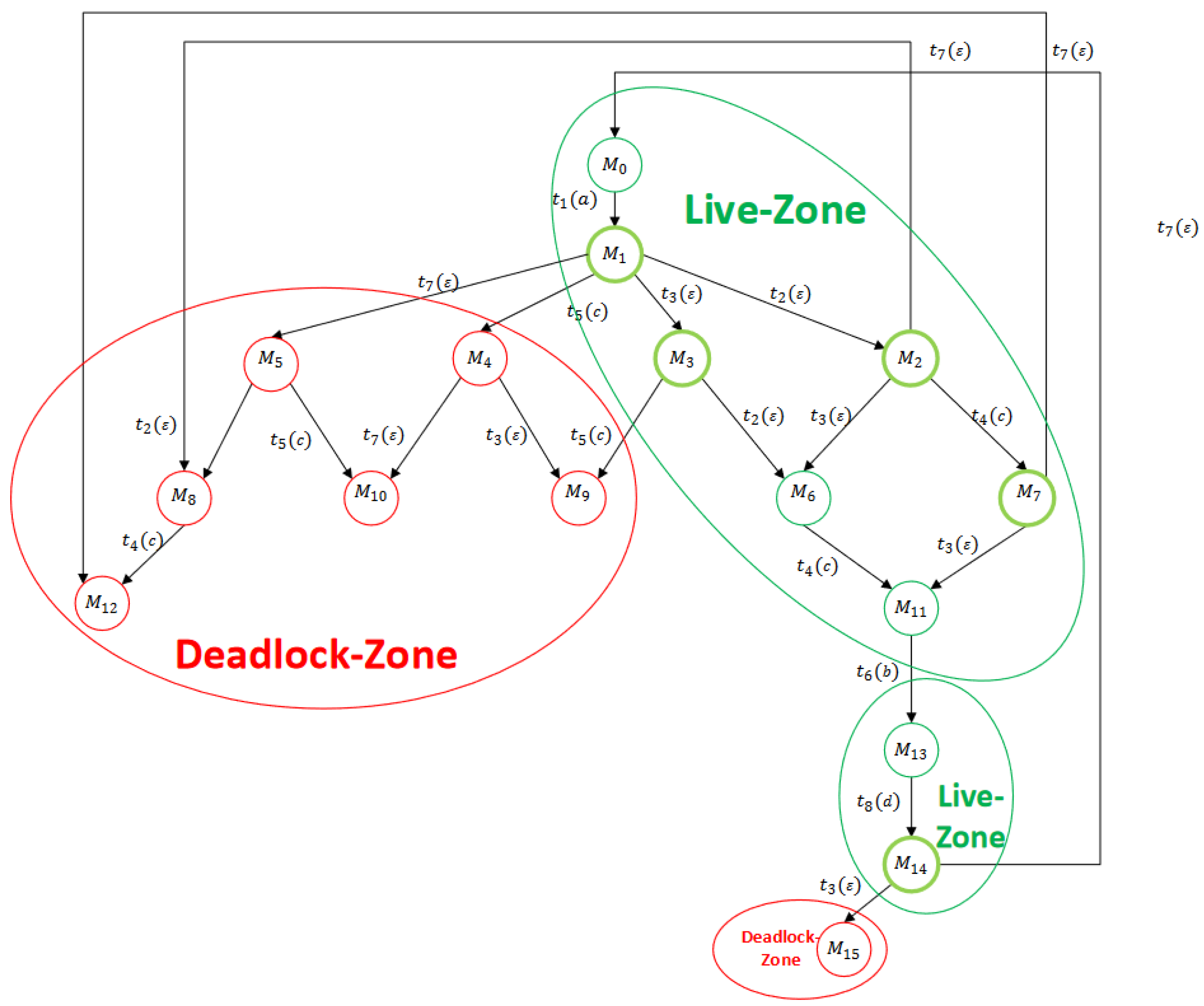
6. Observed Graph: A Deadlock Characterization for Labeled Petri Nets

In this section, we propose a new graph that is able to fully characterize deadlocks in systems modeled by labeled Petri nets.

Definition 8 

(Observed Graph). Given a bounded Petri net $N=(P,T,\mathit{Pre},\mathit{Post})$ with an initial marking $M_0$ and a basis partition $\pi =(T_E,T_I)$, the observed graph of the Petri net is a non-deterministic finite state automaton that is a quadruple $\mathcal{G}=({\mathcal{M}}_O,Tr,{\Delta }_O,M_0)$, where

• the state set ${\mathcal{M}}_O={\mathcal{M}}_B\cup {\mathcal{M}}_D$ is the set of observed markings with:

  –

  the state set ${\mathcal{M}}_B$ being the set of observed basis markings;

  –

  the state set ${\mathcal{M}}_D$ being the set of observed dead markings;

• the event set $Tr$ is the set of pairs $(t,y)\in (T_E\cup \{\varnothing \})\times {\mathbb{N}}^{n_I}$;
• the transition relation is ${\Delta }_O={\Delta }_B\cup {\Delta }_D$ with:

  –

  ${\Delta }_B=\{(M_1,(t,y),M_2)\mid t\in T_E,y\in Y_{min}(M_1,t),\mathit{and}{M}_2=M_1+{\mathcal{C}}_I·y+\mathcal{C}(·,t)\}$

  –

  ${\Delta }_D=\{(M_1,(\varnothing ,y),M_2)\mid y\in {\mathbb{N}}^n,y\in Y_{\beta }\left(M_1\right),\mathit{and}{M}_2=M_1+{\mathcal{C}}_I·y\}$

• the initial state is the initial marking $M_0$.

Algorithm 2 presents a method to calculate the observed graph $\mathcal{G}$. By steps (3–16), we first compute the original BRG. By step 7, the set of entire explanations $Y_T\left(M_b\right)$ is computed. Steps (17–21) check the existence of the sufficient condition given by Theorem 1. If the tested marking M is a DBM, then we add it to the set of dead markings ${\mathcal{M}}_D$, assign a tag to M, and return to step 2 to check another marking without a tag from $M_B$ if there is one. If the first sufficient condition of Theorem 1 is not satisfied by steps (18–21), we check the safeness of the implicit reaches of the marking M. If $\beta$ (the set of dangerous implicit vectors and its corresponding markings computed by Algorithm 1) is not empty, for all $y_I\in \beta$ we add the reachable implicit marking $M_I$ to ${\mathcal{M}}_D$ and $(M,(\varnothing ,y_I),M_I)$ to ${\Delta }_D$. This procedure runs iteratively until there is no unchecked marking in ${\mathcal{M}}_B$. For a bounded Petri net, based on $({\mathcal{M}}_B\cup {\mathcal{M}}_D)\subseteq R(N,M_0)$, Algorithm 2 terminates in a finite time.

Algorithm 2: Construction of observed graph.

Input:  A labeled Petri net $G=(N,M_0,E,\ell )$ and a basis partition $\pi =(T_E,T_I)$  Output:  An observed graph $\mathcal{G}=({\mathcal{M}}_B,{\mathcal{M}}_D,Tr,{\Delta }_B,{\Delta }_D,M_0)$

We first consider the complexity of the observed graph $\mathcal{G}$, i.e., the number of observed markings in it. In the worst case, when each transition in the net system has a self-loop, i.e., the partition $(T_E,T_I)$ is $T_E=T$ and $T_I=\varnothing$, the observed graph $\mathcal{G}$ has the same complexity as the basis reachability graph and the reachability graph, i.e., $|{\mathcal{M}}_B|=|{\mathcal{M}}_O|=|R(N,M_0)|$. In plain words, the complexity of Algorithm 2 is exponential with respect to a plant. Despite in the aforementioned case that the computation of $\mathcal{G}$ shares the same complexity as a reachability graph and a BRG, there always exists a basis partition $(T_E,T_I)$ with the implicit transition set not being empty such that $\mathcal{G}$ is as small as possible in size, i.e., $|{\mathcal{M}}_O|\ll |R(N,M_0)|$ and more precisely $|{\mathcal{M}}_B|\le |{\mathcal{M}}_O|\le |{\mathcal{M}}_B|+|\mathcal{D}|$, where $\left|\mathcal{D}\right|$ represents the number of dead markings. Such a partition can be found via offline simulation or decided by the sensor configuration of a real system.

Theorem 5. 

Given an LPN $G=(N,M_0,E,\ell )$ and its observed graph $\mathcal{G}=({\mathcal{M}}_O,Tr,{\Delta }_O,M_0)$, if there is no dead marking in $\mathcal{G}$, G is a deadlock-free net.

Proof. 

This is trivial. Suppose that the observed graph of G does not contain any dead observed markings. There is no marking in G that can be a deadlock state at which no transition is enabled, which completes the proof. □

Example 5. 

Consider again the Petri net system given by Figure 8. The set of deadlock markings is $\mathcal{D}=\{M_{D1}=\left[000002001\right],M_{D2}=\left[100001000\right],M_{D3}=\left[100010000\right],M_{D4}=\left[000001102\right]\}$. In Figure 10, we present the BRG composed of six markings. However, only one dead marking $M_{b3}=\left[001001001\right]$ exists in the BRG.

Using Algorithm 2, we construct the observed graph of the Petri net system. The resulting graph is shown in Figure 11, which contains eight markings. From $M_{b2}=\left[001010001\right]$, the set of DIVS and DIMs are $\beta =\mathsf{\Psi }\left(M_{b2}\right)=\left[100010000\right|001]$. By steps (20–21), we add $M_{D1}=\left[100010000\right]$ to ${\mathcal{M}}_D$ and $(M_{b2},(\varnothing ,\left[001\right]),M_{D1})$ to ${\Delta }_D$. However, $M_{b3}=\left[001001001\right]$ is defined as a dead basis marking (DBM). Since $Y_T\left(M_{b3}\right)=\varnothing$, we tag $M_{b3}$ as an old node and execute step 2 to check the existence of a marking without a tag in ${\mathcal{M}}_B$. Considering Theorem 1, there is no need to check the safeness of the implicit reaches of $M_{b3}$. Similar to $M_{b2}$, at $M_{b5}$ we have $\beta \ne \varnothing$ and its value is $\beta =\left[000001102\right|010]$. Thus, a new node $M_{d2}=\left[000001102\right]$ and a new relation $(M_{b5},(\varnothing ,\left[010\right]),M_{d2})$ will be added to ${\mathcal{M}}_D$ and ${\Delta }_D$, respectively.

Figure 11. Observed graph of the LPN in Example 2.

The proposed approach to deadlock characterization and analysis of labeled Petri nets can be algorithmically scheduled as follows. Given a labeled Petri net, we first construct its BRG provided that the $T_{uo}$-induced subset is acyclic, leading to a basis partition $(T_E,T_I)$ with $T_I=T_{uo}$ and $T_E=T-T_I$. Then, based on the BRG, a structure called an observed graph is constructed, which contains deadlock-related information, in which dangerous implicit markings and dangerous implicit vectors are full indicators associated with deadlocks. If there is no dead marking in the observed graph, we conclude that there is no deadlock in the original labeled Petri net.

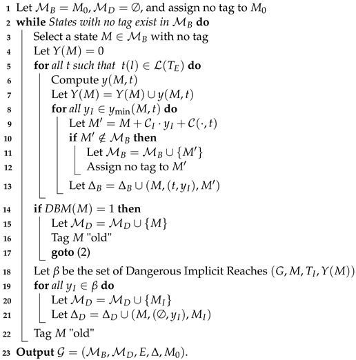
7. Experimental Results

In this section, we will introduce the experimental results of this work. A flexible manufacturing system is used to illustrate the proposed deadlock characterization policy for labeled Petri nets. The Petri net model of the system shown in Figure 12 is a pure and bounded Petri net taken from [46].

Figure 12. Labeled Petri net of Example 3.

In the net, there are 13 places $\{p_0,\cdots ,p_{12}\}$ and 10 transitions $\{t_0,\cdots ,t_9\}$. Given the system partition $\pi =(T_E,T_I)$ with $T_E=T_o=\{t_1\left(a\right),t_2\left(b\right),t_3\left(b\right),t_4\left(a\right),t_5\left(c\right),t_8\left(c\right)\}$ and $T_I=T_{uo}=\{t_0\left(\epsilon \right),t_6\left(\epsilon \right),t_7\left(\epsilon \right),t_9\left(\epsilon \right)\}$ and the initial marking $M_0=2p_0+p_5+p_6+2p_7+p_{11}+p_{12}$, Figure 13 shows that the net has thirty-two reachable markings, twenty-eight of which are legal markings depicted in solid lines and four of which are deadlock ones depicted in dashed lines. The set of deadlock markings is $\mathcal{D}=\{M_{D_1}=2p_0+p_5+p_6+p_8+p_9,M_{D_2}=p_0+p_2+p_6+p_8+p_9,M_{D_3}=p_2+p_3+p_8+p_9,M_{D_4}=p_0+p_3+p_5+p_8+p_9\}$.

Figure 13. Reachability graph of the LPN in Example 3.

In Figure 14, we present the basis reachability graph of the net system. As the BRG shows, the number of basis markings is $\left|\mathcal{M}\right|=11$. However, none of the dead markings appears in the BRG, i.e., for all $M\in \mathcal{D}$, $M\notin \mathcal{M}$. We construct the observed graph with Algorithm 2. The number of markings is $|{\mathcal{M}}_O|=15$. We observe that $\left|\mathcal{M}\right|\le \left|{\mathcal{M}}_O\right|\le |R(N,M_0)|$ and $\mathcal{M}\subseteq {\mathcal{M}}_O\subseteq R(N,M_0)$. From the marking $M_{b0}$, we have $\beta =\left[2000011011000\right|0,2,1,0].$ Thus, the dead markings $M_{d0}$ is added to the observed graph since it represents a dangerous implicit reachable marking. In the same way as $M_{b1}$, the computation of the set of DIVs and DIMs results in $\beta =\left[1010001011000\right|0,2,1,0]$ and a new dead node $M_{d1}=\left[1010001011000\right]$ is added. From the marking $M_{b2}$, we also have a dangerous implicit reach given by $M_{d2}=\left[1001010011000\right]$ thanks to $\beta =\left[1001010011000\right|0,2,1,0].$ Finally, from the marking $M_{b4}$, $\beta =\left[0011000011000\right|0,2,1,0]$ is obtained, and a dead observed marking $M_{d3}=\left[0011000011000\right]$ is added to the observed graph (see Figure 15).

Figure 14. BRG of the LPN in Example 3.

Figure 15. Observed graph of the LPN in Example 3.

From this example, it is found that a BRG fails to fully expose the dead markings in a labeled Petri net, while the proposed observed graph can capture the dead markings. The reason that a BRG is capable of addressing fault diagnosis of DESs seems obvious: A fault is usually treated as an unobservable transition since, otherwise, its occurrence can be immediately observed after it happens such that the BRG does not lose any useful information for diagnosability analysis. For deadlock characterization and analysis, a system may unobservably reach a deadlock state without any observational indicator, rendering that a BRG needs to be modified, and the observed graphs are developed in this research.

8. Conclusions and Future Work

This paper addresses the deadlock characterization and analysis in labeled Petri nets whose transitions can be unobservable and undistinguishable. In the first part of the paper, we show that the notion of BRG cannot correctly and accurately define and characterize the deadlock problem in an LPN. We propose a first algorithm to compute the max-cardinality of the implicit vector, which can fire from a given state of the system. After that, we introduce two sufficient conditions described by linear algebraic equations, which will be useful for constructing the observed graph. Then, we provide an algorithm for computing the observed graph. Finally, experimental results implemented using the C # tool confirmed the correctness and effectiveness of the proposed solution. To move forward, future research in this framework will focus on using observed graphs to ensure the deadlock-freeness and to study the liveness enforcement of systems modeled by labeled Petri nets.

It is also interesting to explore deadlock analysis and detection approaches for a DES that is subject to external malicious attacks. An attack can delete and replace a label in an observation in such a way that the observed graph established in this research is not real. To this end, a robust deadlock characterization and analysis method is needed.

References

- Cassandras, C.G.; Lafortune, S. Introduction to Discrete Event Systems, 2nd ed.; Springer: New York, NY, USA, 2008. [Google Scholar]
- Liang, Y.; Liu, G.Y.; El-Sherbeeny, A.M. Polynomial-time verification of decentralized fault pattern diagnosability for discrete-event systems. Mathematics 2023, 11, 3398. [Google Scholar] [CrossRef]
- Li, Y.Y.; Chen, Y.F.; Zhou, R. A set covering approach to design maximally permissive supervisors for flexible manufacturing systems. Mathematics 2024, 12, 1687. [Google Scholar] [CrossRef]
- Dou, H.; You, D.; Wang, S.G.; Zhou, M.C. Designing liveness-enforcing supervisors for manufacturing systems by using maximally good step graphs of Petri nets. IEEE Trans. Autom. Sci. Eng. 2024, 1–12. [Google Scholar] [CrossRef]
- Zhang, R.P.; Feng, Y.X.; Yang, Y.K.; Li, X.L.; Li, H.N. Polynomial-complexity deadlock avoidance policy for tasks offloading in satellite edge computing with data-dependent constraints and limited buffers. IEEE Trans. Aerosp. Electron. Syst. 2024, 60, 6822–6838. [Google Scholar] [CrossRef]
- Qi, H.D.; Wang, J.L.; Yan, C.G.; Jiang, C.J. The probabilistic liveness decision method of unbounded Petri nets based on machine learning. IEEE Trans. Syst. Man Cybern. Syst. 2024, 54, 1070–1081. [Google Scholar] [CrossRef]
- Zhang, L.; Holloway, L.E. Forbidden state avoidance in controlled Petri nets under partial observation. In Proceedings of the 33rd Allerton Conference on Communication, Control, and Computing, Monticello, IL, USA, 27–29 September 1995; pp. 146–155. [Google Scholar]
- Li, Y.; Wonham, W.M. Controllability and observability in the state-feedback control of discrete-event systems. In Proceedings of the 27th IEEE Conference on Decision and Control, Austin, TX, USA, 7–9 December 1989; pp. 203–208. [Google Scholar]
- Zhou, Y.; Hu, H.S.; Deng, G.L.; Cheng, K.; Lin, S.W.; Liu, Y.; Ding, Z.H. Distributed motion control for multiple mobile robots using discrete-event systems and model predictive control. IEEE Trans. Syst. Man Cybern. Syst. 2024, 54, 997–1010. [Google Scholar] [CrossRef]
- Basile, F.; Chiacchio, P.; Giua, A.; Seatzu, C. Deadlock recovery of Petri net models controlled using observers. In Proceedings of the 8th IEEE Conference on Emerging Technologies and Factory Automation, Antibes, France, 15–18 October 2001; pp. 441–449. [Google Scholar]
- Giua, A.; Seatzu, C. Deadlock characterization for Petri nets controlled using GMECs and observers. In Proceedings of the 2003 American Control Conference, Denver, CO, USA, 4–6 June 2003; pp. 320–325. [Google Scholar]
- Wonham, W.; Cai, K. Supervisory Control of Discrete-Event Systems; Springer: Cham, Switzerland, 2018. [Google Scholar]
- Li, Z.; Zhao, M. On controllability of dependent siphons for deadlock prevention in generalized Petri nets. IEEE Trans. Syst. Man Cybern. A Syst. Hum. 2008, 38, 369–384. [Google Scholar]
- Li, Z.; Zhang, J.; Zhao, M. Liveness-enforcing supervisor design for a class of generalised Petri net models of flexible manufacturing systems. IET Control Theory Appl. 2007, 1, 955–967. [Google Scholar] [CrossRef]
- Chen, Y.F.; Li, Z.W. On structural minimality of optimal supervisors for flexible manufacturing systems. Automatica 2012, 48, 2647–2656. [Google Scholar] [CrossRef]
- Ezpeleta, J.; Colom, J.M.; Martinez, J.A. A Petri net based deadlock prevention policy for flexible manufacturing systems. IEEE Trans. Robot. Autom. 1995, 11, 173–184. [Google Scholar] [CrossRef]
- Fanti, M.P.; Zhou, M.C. Deadlock control methods in automated manufacturing systems. IEEE Trans. Syst. Man Cybern. A Syst. Hum. 2004, 34, 5–22. [Google Scholar] [CrossRef]
- Lautenbach, K.; Ridder, H. The Linear Algebra of Deadlock Avoidance–A Petri Net Approach; Tech. Rep. No. 25–96; Institute of Software Technology, University of Koblenz-Landau: Koblenz, Germany, 1996. [Google Scholar]
- Wang, S.G.; You, D.; Wang, C.Y. Optimal supervisor synthesis for Petri nets with uncontrollable transitions: A bottom-Up algorithm. J. Inf. Sci. 2016, 363, 261–273. [Google Scholar] [CrossRef]
- Xing, K.Y.; Zhou, M.C.; Wang, F.; Liu, H.X.; Tian, F. Resource-transition circuits and siphons for deadlock control of automated manufacturing systems. IEEE Trans. Syst. Man Cybern. A Syst. Hum. 2011, 41, 74–84. [Google Scholar] [CrossRef]
- Ezpeleta, J.; Rcalde, L. A deadlock avoidance approach for non-sequential resource allocation systems. IEEE Trans. Syst. Man Cybern. A Syst. Hum. 2004, 34, 93–101. [Google Scholar] [CrossRef]
- Hsieh, F.S. Fault-tolerant deadlock avoidance algorithm for assembly processes. IEEE Trans. Syst. Man Cybern. A Syst. Hum. 2004, 34, 65–79. [Google Scholar] [CrossRef]
- Wu, N.Q.; Zhou, M.; Li, Z.W. Resource oriented Petri net for deadlock avoidance in flexible assembly systems. IEEE Trans. Syst. Man Cybern. A Syst. Hum. 2008, 38, 56–69. [Google Scholar]
- Wu, N.Q.; Zhou, M.C. Modeling, analysis and control of dual-arm cluster tools with residency rime constraint and activity time variation based on Petri nets. IEEE Trans. Autom. Sci. Eng. 2012, 9, 446–454. [Google Scholar]
- Wu, N.Q.; Zhou, M.C. Schedulability analysis and optimal scheduling of dual-arm cluster tools with residency time constraint and activity time Variation. IEEE Trans. Autom. Sci. Eng. 2012, 9, 203–209. [Google Scholar]
- Xing, K.Y.; Zhou, M.C.; Liu, H.X.; Tian, F. Optimal Petri-net-based polynomial-complexity deadlock-avoidance policies for automated manufacturing systems. IEEE Trans. Syst. Man Cybern. A Syst. Hum. 2009, 39, 188–199. [Google Scholar] [CrossRef]
- Dotoli, M.; Fanti, M.P. Deadlock detection and avoidance strategies for automated storage and retrieval systems. IEEE Trans. Syst. Man Cybern. C Appl. Rev. 2007, 37, 541–552. [Google Scholar] [CrossRef]
- Huang, Y.S.; Pan, Y.L.; Su, P.J. Transition-based deadlock detection and recovery policy for FMSs using graph technique. ACM Trans. Embed. Comput. Syst. 2013, 12, 11:1–11:13. [Google Scholar] [CrossRef]
- Kumaran, T.K.; Chang, W.; Cho, H.; Wysk, R.A. A structured approach to deadlock detection, avoidance and resolution in flexible manufacturing systems. Int. J. Prod. Res. 1994, 32, 2361–2379. [Google Scholar] [CrossRef]
- Wysk, R.A.; Yang, N.S.; Joshi, S. Resolution of deadlocks in flexible manufacturing systems: Avoidance and recovery approaches. J. Manuf. Syst. 1994, 13, 128–138. [Google Scholar] [CrossRef]
- Chen, Y.; Li, Z.W.; Al-Ahmari, A.; Wu, N.Q.; Qu, T. Deadlock recovery for flexible manufacturing systems modeled with Petri nets. J. Inf. Sci. 2017, 381, 290–303. [Google Scholar] [CrossRef]
- Giua, A.; Seatzu, C.; Basile, F. Observer-based state-feedback control of timed Petri nets with deadlock recovery. IEEE Trans. Autom. Control 2004, 49, 17–29. [Google Scholar] [CrossRef]
- Chen, F.; Barkaoui, K. Maximally permissive Petri net supervisors for flexible manufacturing systems with uncontrollable and unobservable transitions. Asian J. Control 2014, 16, 1646–1658. [Google Scholar] [CrossRef]
- Corona, D.; Giua, A.; Seatzu, C. Marking estimation of Petri nets with silent transitions. In Proceedings of the 43rd IEEE Conference on Decision and Control, Paradise Island, Bahamas, 14–17 December 2004; pp. 966–971. [Google Scholar]
- Ren, K.X.; Zhang, Z.P.; Xia, C.Y. Event-based fault diagnosis of networked discrete event systems. IEEE Trans. Circuits Syst. II Express Briefs 2022, 69, 1787–1791. [Google Scholar] [CrossRef]
- Murata, T. Petri nets: Properties, analysis, and applications. Proc. IEEE 1989, 77, 541–580. [Google Scholar] [CrossRef]
- Zaghdoud, A.; Li, Z. Preliminaries of Finite State Automata and Petri Nets. 2024. Available online: https://github.com/Zhiwuli/File/blob/main/Preliminaries_FSA_and_LPN.pdf (accessed on 1 September 2024).
- Peterson, J.L. Petri Net Theory and the Modelling of Systems; Prentice-Hall: Rutherford, NJ, USA, 1981. [Google Scholar]
- Cabasino, M.; Giua, A.; Seatzu, C. Fault detection for discrete event systems using Petri nets with unobservable transitions. Automatica 2010, 46, 1531–1539. [Google Scholar] [CrossRef]
- Cabasino, M.; Giua, A.; Pocci, M.; Seatzu, C. Discrete event diagnosis using labeled Petri nets: An application to manufacturing systems. Control Eng. Pract. 2011, 19, 989–1001. [Google Scholar] [CrossRef]
- Tong, Y.; Li, Z.W.; Seatzu, C.; Giua, A. Verification of state-based opacity using Petri nets. IEEE Trans. Autom. Control 2017, 62, 2823–2837. [Google Scholar] [CrossRef]
- Ma, Z.Y.; Tong, Y.; Li, Z.W.; Giua, A. Basis marking representation of Petri net reachability spaces and its application to the reachability problem. IEEE Trans. Autom. Control 2017, 62, 1078–1093. [Google Scholar] [CrossRef]
- Uzam, M.; Zhou, M.C. An improved iterative synthesis method for liveness enforcing supervisors of flexible manufacturing systems. Int. J. Prod. Res. 2006, 44, 1987–2030. [Google Scholar] [CrossRef]
- Chen, Y.; Li, Z.W.; Barkaoui, K. Maximally permissive Petri net supervisors with a novel structure. In Proceedings of the 12th IFAC/IEEE International Workshop on Discrete Event Systems, Cachan, France, 14–16 May 2014; pp. 80–85. [Google Scholar]
- Chen, Y.F.; Li, Z.W.; Al-Ahmari, A. Nonpure Petri net supervisors for optimal deadlock control of flexible manufacturing systems. IEEE Trans. Syst. Man Cybern. Syst. 2013, 43, 252–265. [Google Scholar] [CrossRef]
- Zhang, X.; Uzam, M. Transition-based deadlock control policy using reachability graph for flexible manufacturing systems. Adv. Mech. Eng. 2016, 8, 1–9. [Google Scholar] [CrossRef]
Disclaimer/Publisher’s Note: The statements, opinions and data contained in all publications are solely those of the individual author(s) and contributor(s) and not of MDPI and/or the editor(s). MDPI and/or the editor(s) disclaim responsibility for any injury to people or property resulting from any ideas, methods, instructions or products referred to in the content. |
© 2024 by the authors. Licensee MDPI, Basel, Switzerland. This article is an open access article distributed under the terms and conditions of the Creative Commons Attribution (CC BY) license (https://creativecommons.org/licenses/by/4.0/).