The Refinement of a Common Correlated Effect Estimator in Panel Unit Root Testing: An Extensive Simulation Study

Abstract

The Common Correlated Effect (CCE) estimator is widely used in panel data models to address cross-sectional dependence, particularly in nonstationary panels. However, existing estimators have limitations, especially in small-sample settings. This study refines the CCE estimator by introducing new proxy variables and testing them through a comprehensive set of simulations. The proposed method is simple yet effective, aiming to improve the handling of cross-sectional dependence. Simulation results show that the refined estimator eliminates cross-sectional dependence more effectively than the original CCE, with improved power properties under both weak- and strong-dependence scenarios. The refined estimator performs particularly well in small sample sizes. These findings offer a more robust framework for panel unit root testing, enhancing the reliability of CCE estimators and contributing to further developments in addressing cross-sectional dependence in panel data models.

1. Introduction

Economists have increasingly focused on testing the stationarity properties of variables in panel data —e.g., [1,2,3,4,5,6,7,8,9] (refs. [10,11,12] provide a comprehensive review of the literature on unit roots and cointegration in panels). Panel data techniques for testing unit roots were developed to address the low power of conventional unit root tests by utilizing both time and cross-sectional dimensions [12]. The most widely used panel unit root tests, such as those proposed by [5,13] (henceforth, IPS), are extensions of [14]’s test into a panel setting.

As pointed out by [12], the assumption of cross-sectional independence might be too restrictive, especially in cross-country or cross-region regressions. Cross-sectional dependence may arise from spatial correlations, spill-over effects, omitted global variables, common unobserved shocks, or residual interdependence after accounting for common factors. This dependence invalidates classical unit root and cointegration tests in panel data models. Studies by [2,15,16] demonstrate through simulations that panel unit root tests that ignore cross-sectional dependence perform poorly when applied to correlated panels.

Cross-sectional correlation is typically modeled using either common unobserved factors or general correlations among individual-specific innovations. Studies such as [2,6,17,18,19,20,21] have used bootstrap methods to address cross-sectional correlation in panel unit root tests. Alternatively, ref. [22] proposed a nonlinear instrumental variable approach to handle general forms of cross-sectional dependence (henceforth, CSD). Assuming CSD arises from common unobserved factors, refs. [23,24,25,26] applied the principal component method to estimate these factors and their loadings. Meanwhile, refs. [8,9] augmented individual ADF tests with cross-sectional averages to proxy for the common factor, rather than estimating it directly (when the size of time dimension ($T$) is large relative to the cross-section dimension ($N$) of the panel, cross-sectional dependency may be accounted for using standard time series techniques applied to systems of equations, for example, the seemingly unrelated regression equation (SURE) approach).

Each of the methods mentioned above poses practical challenges. In the context of panel data, the Common Correlated Effect (CCE) estimator proposed by [27] offers an alternative for addressing cross-sectional dependence from unobserved common shocks or factors. By using cross-sectional averages of the dependent and independent variables, CCE captures these shared shocks, leading to more consistent and reliable estimates without advanced techniques. Refining CCE estimators is essential for improving accuracy, especially in small samples, and for handling complex data structures like nonlinearity or structural breaks, while also reducing bias from correlations between regressors and common factors.

While [8]’s methodology has been widely studied for its power and size properties, [28] showed that the CCE estimator provides consistent and asymptotically normal estimates, even with a multifactor error structure. Despite this, recent studies have highlighted its limitations. For instance, [29] criticized the CCE estimator’s assumption of independence between common factors and regressors, arguing that the $\left(k+1\right)$ factor estimated by CCE may be insufficient and that asymptotic normality breaks down when $r>\left(k+1\right)$.

Our study addresses these shortcomings by proposing a refinement to the CCE estimator, introducing new proxy variables that are simpler and more effective at capturing cross-sectional dependence. Unlike previous methods, our approach reduces the correlation between regressors and proxy factors, which has been a critical drawback of the CCE estimator. Through an extensive simulation study, we demonstrate that our refined method improves performance, particularly in small sample sizes, and better handles both weak and strong dependence. This novel approach contributes to the ongoing refinement of CCE estimators and offers a more robust framework for panel unit root testing. To address these issues, we conducted the simulation study described below.

We use [30]’s cross-sectional dependency test (henceforth, $C{D}_{LM}$ test) to assess whether our new estimator effectively remedies cross-sectional dependency. The use of the $C{D}_{LM}$ test in this simulation study proved to be highly convenient. First, we verified that the $C{D}_{LM}$ test accurately detected the CSD present in the data-generating process (henceforth, DGP). In the next stage, the $C{D}_{LM}$ test confirmed the absence of CSD when no CSD was present. We then introduced generated factor data, and the $C{D}_{LM}$ test showed that adding the factor eliminated CSD. However, when we applied the CCE estimator by [27], it was clear that it did not fully remove CSD. In contrast, our refined CCE estimator successfully eliminated CSD and bias. As noted by [31], the CCE estimator can mistakenly capture common structural breaks instead of factors when there is a common trend or break in the DGP, raising concerns about adding extra factors as proposed by [29]. Similarly, [32] emphasized that structural breaks could be mistaken for common factors, leading to model misspecification. Instead of complicating the CCE estimator as mentioned in [29], we refined it by using the simple average of the original data (${\overline{y}}_t$) in the auxiliary regression instead of using $∆{\overline{y}}_t$ (the panel unit root tests’ dependent variable) and the independent variable. This approach reduces the correlation between regressors and proxy factor variables, addressing the main drawback of the CCE estimator, as highlighted by [29]. While the new method performed well for small $N$, it was less effective for larger $N$. Thus, we proposed a two-stage estimator: first, using the CCE estimator to reduce correlation issues, and second, applying an auxiliary regressor generated in the first stage. In the empirical section, we compared the new unit root test with [8]’s test using data with structural breaks. While [8]’s test incorrectly indicated stationarity, the new test identified the unit root problem, eliminating size bias.

The rest of the study is organized as follows: Section 2 explains the new refinement methodology and simulations; and introduces the new panel unit root test and the small-sample results; Section 3 presents the empirical results; and Section 4 is the conclusion.

2. The Panel Unit Root Test and the Refinement of the CCE Estimator

2.1. Common Correlated Estimator in Panel Unit Root Testing

In this part, we introduce a practical way to refine the CCE estimator of [8]. In the author’s well-known paper, he introduces an auxiliary regression to remedy cross-sectional dependency. In line with [8], we consider the following heterogeneous panel ADF regression:

$$∆y_{it}={\beta }_i{y}_{i,t-1}+{\epsilon }_{it}$$

(1)

$${\epsilon }_{it}={\lambda }_i{f}_t+u_{it}$$

(2)

$$\mathrm{with} {\epsilon }_{it}~i.i.d.N\left(0,{\sigma }_i^2\right)\mathrm{and} f_t~N\left(0,{\sigma }_f^2\right)$$

where $f_t$ is the unobserved common factor assumed to be a stationary process, ${\lambda }_i$ is factor loadings, and $u_{it}$ is the individual specific error terms. For the moment, we assume that idiosyncratic error terms $u_{it}$ are independently distributed across both $i$ and $t$.

The common factor $f_t$ can be proxied by the cross-sectional mean of $∆y_{it}$ and ${\mathrm{y}}_{\mathrm{i},\mathrm{t}-1}$ following [8,27]. To see this, first re-write Equation (1) as follows:

$$∆y_{it}={\beta }_i{y}_{i,t-1}+{\lambda }_i{f}_t+u_{it}$$

(3)

Taking the cross-section average of both sides, we obtain the following equation:

$$∆{\overline{y}}_t=\overline{\beta }{\overline{y}}_{t-1}+\overline{\lambda }{f}_t+{\overline{u}}_t+N^{-1}\sum \left({\beta }_i-\overline{\beta }\right)y_{i,t-1}$$

(4)

Assuming that $\overline{\lambda }=N^{-1}\sum _{i=1}^N{\lambda }_i$ does not vanish, the common factor $f_t$ can be written as

$$f_t={\displaystyle \frac{1}{\overline{\lambda }}}\left[∆{\overline{y}}_t-\overline{\beta }{\overline{y}}_{t-1}-{\overline{u}}_t-N^{-1}\sum \left({\beta }_i-\overline{\beta }\right)y_{i,t-1}\right]$$

(5)

which suggests that the common factor can be proxied by a linear combination of $∆{\overline{y}}_t$ and ${\overline{y}}_{t-1}$. Therefore, in order to filter out the effects of the common factor, we run the following modified test regression:

$$∆y_{it}=b_i{y}_{i,t-1}+c_i{\overline{y}}_{t-1}+d_i∆{\overline{y}}_t+e_{it}$$

(6)

Then, the test of the null hypothesis of the unit root ($H_0:{\beta }_i=0$ in Equation (1) above) is based on $t-$ ratio of the OLS estimate of $b_i$ in Equation (6).

In Equation (1) and hence in Equation (6), it was assumed that the error terms are not serially correlated. In order to allow for serial correlation in the error terms, we ran the following augmented regression:

$$∆y_{it}=b_i{y}_{i,t-1}+c_i{\overline{y}}_{t-1}+\sum _{j=0}^p{d}_{ij}∆{\overline{y}}_{t-j}+\sum _{j=1}^p{\delta }_{ij}∆y_{i,t-j}+e_{it}$$

(7)

and we compute the test statistic from Equation (7) (see [8]).

Ref. [28] demonstrated that the CCE estimator provides consistent and asymptotically normal estimates of slope coefficients in panel data models, even with a multifactor error structure. In this section, we aim to explore additional properties by using the CSD test to determine whether the CCE estimator truly remedies the CSD issue. To carry out this, we employ the $C{D}_{LM}$ test from [30]. First, we need to verify if this test performs well across different levels of CSD.

2.2. The Behavior or Performance of the $C{D}_{LM}$ Test

In this section, we first conduct a Monte Carlo study to test whether the $C{D}_{LM}$ test works properly with DGP given in Equation (3). The features of this DGP are described in [8,27], where CSD is introduced into the panel data using a factor structure, as shown in Equation (3). First, we compute the $C{D}_{LM}$ test directly on the DGP to verify if the test detects CSD. In the second stage, we use the same DGP but apply the factor structure to remedy the CSD during the testing process. We expect to observe severe CSD in the first Monte Carlo setup and no CSD in the second. If these expectations hold, the $C{D}_{LM}$ test can be used to assess the CCE estimator proposed by [8,27]. Previous studies [28] have shown that the CCE estimator effectively remedies CSD and produces unbiased estimates. While our analysis complements theirs, our findings suggest a new direction for developing a more efficient estimator. In the final stage, we propose a new estimator based on these new insights.

The Monte Carlo design used in this study can be summarized as follows: First, we generate data using Equation (3) with factor loadings ${\lambda }_i$ ranging from −1.0 to 3.0, as suggested by the authors of [8,27], who classify this range as strong CSD. In our study, we compute the $C{D}_{LM}$ test for each factor loading in this interval at 0.1 increments. These computations are performed for $N=\left\{\mathrm{10,50,100}\right\}$ and $T=\left\{\mathrm{10,20,30,40,50,60,80,100,200}\right\}$. For each point, we calculate the $C{D}_{LM}$ test 1000 times to examine the distribution and the minimum and maximum values of the test. For example, with $N=10$ and $T=10$, we generate 40 intervals representing the probability of detecting CSD when imposed or, conversely, detecting no CSD. For $N=\left\{\mathrm{10,50,100}\right\}$ and $T=\left\{\mathrm{10,20,30,40,50,60,80,100,200}\right\}$ values as described, this results in 360 cells ($40\times 3\times 9$), which can be displayed in 27 tables for each $N$ and $T$. 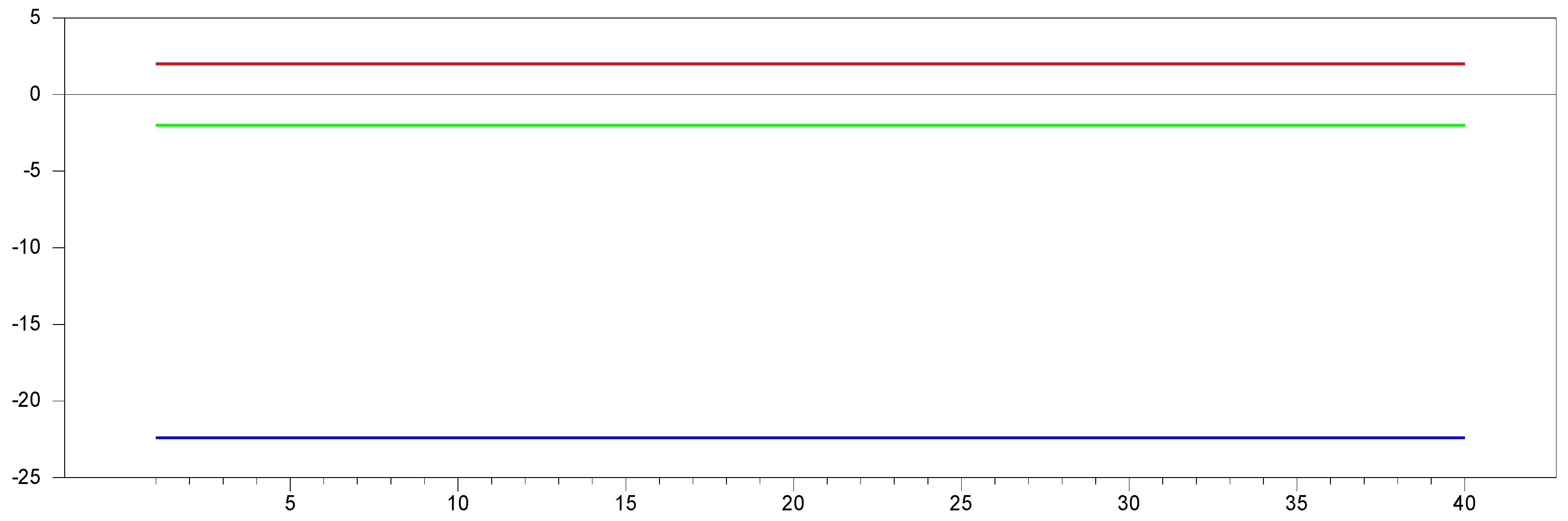To simplify interpretation, we present the results visually through figures. In these figures, we also include the 10% significance interval for the z-test, ranging from −2.0 to 2.0.

We consider the following panel regression model,

$$\mathsf{\Delta }{y}_{it}={\mu }_i+{\beta }_i{x}_{it}+u_{it}$$

(8)

for $i=1,\dots ,N$ cross-sectional units and $t=1,\dots ,T$ time periods. The sample estimate of the pair-wise correlation of the residuals is given by

$${\widehat{\rho }}_{ij}={\widehat{\rho }}_{ji}={\displaystyle \frac{\sum _{t=1}^T{e}_{it}{e}_{jt}}{{\left(\sum _{t=1}^T{e}_{it}^2\right)}^{\frac{1}{2}}{\left(\sum _{t=1}^T{e}_{jt}^2\right)}^{1/2}}}$$

(9)

where $e_{it}$ is the OLS estimates of $u_{it}$ defined as $e_{it}={\widehat{u}}_{it}=\mathsf{\Delta }{y}_{it}-{\widehat{\mu }}_i+{\widehat{\beta }}_i{x}_{it}$. Ref. [30] suggests that the $C{D}_{LM}$ test statistic can be computed as

$$C{D}_{LM}=\sqrt{{\displaystyle \frac{2T}{N\left(N-1\right)}}}\left(\sum _{i=1}^{N-1}\sum _{j=i+1}^N{\widehat{\rho }}_{ij}\right)$$

(10)

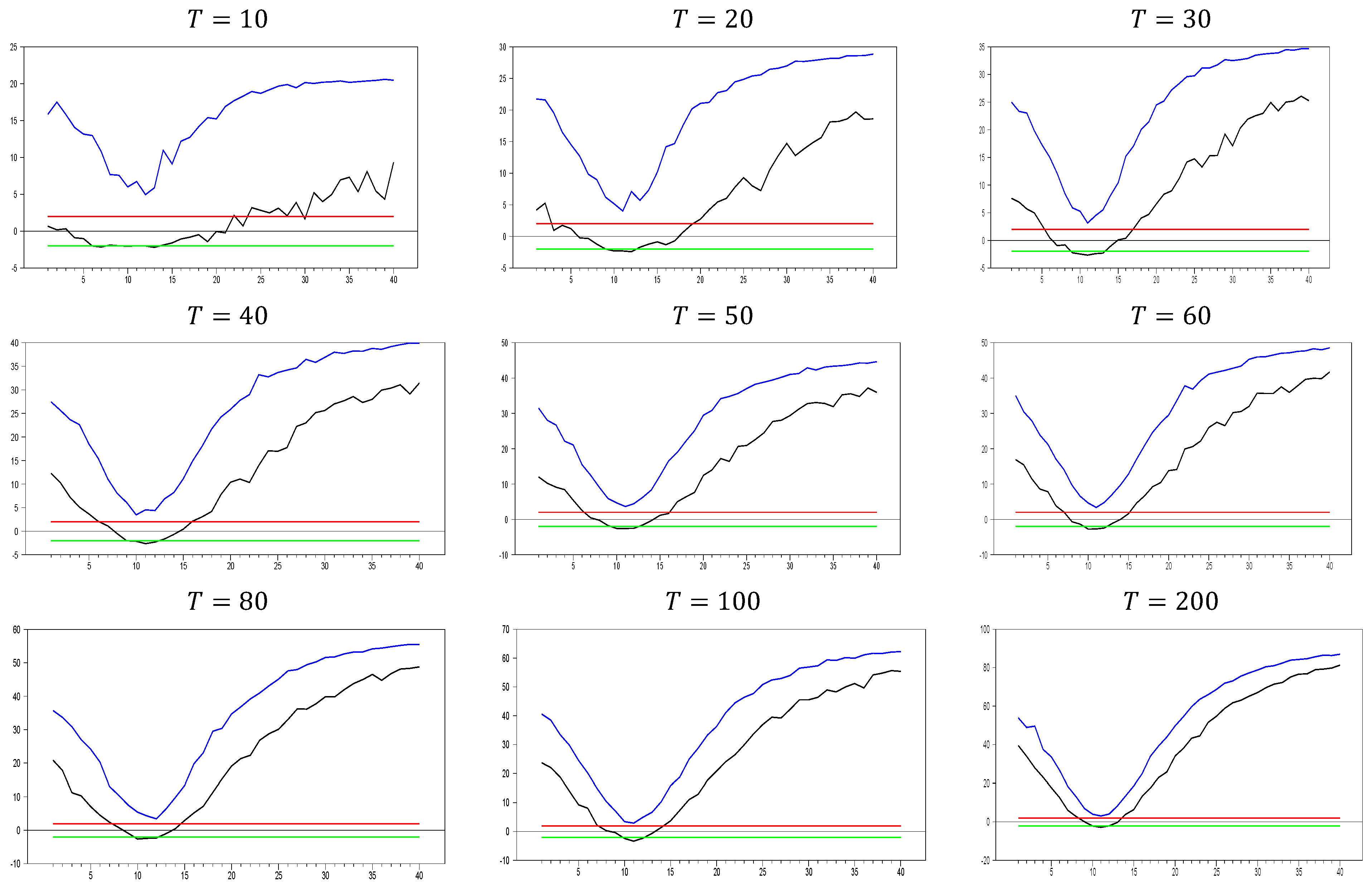
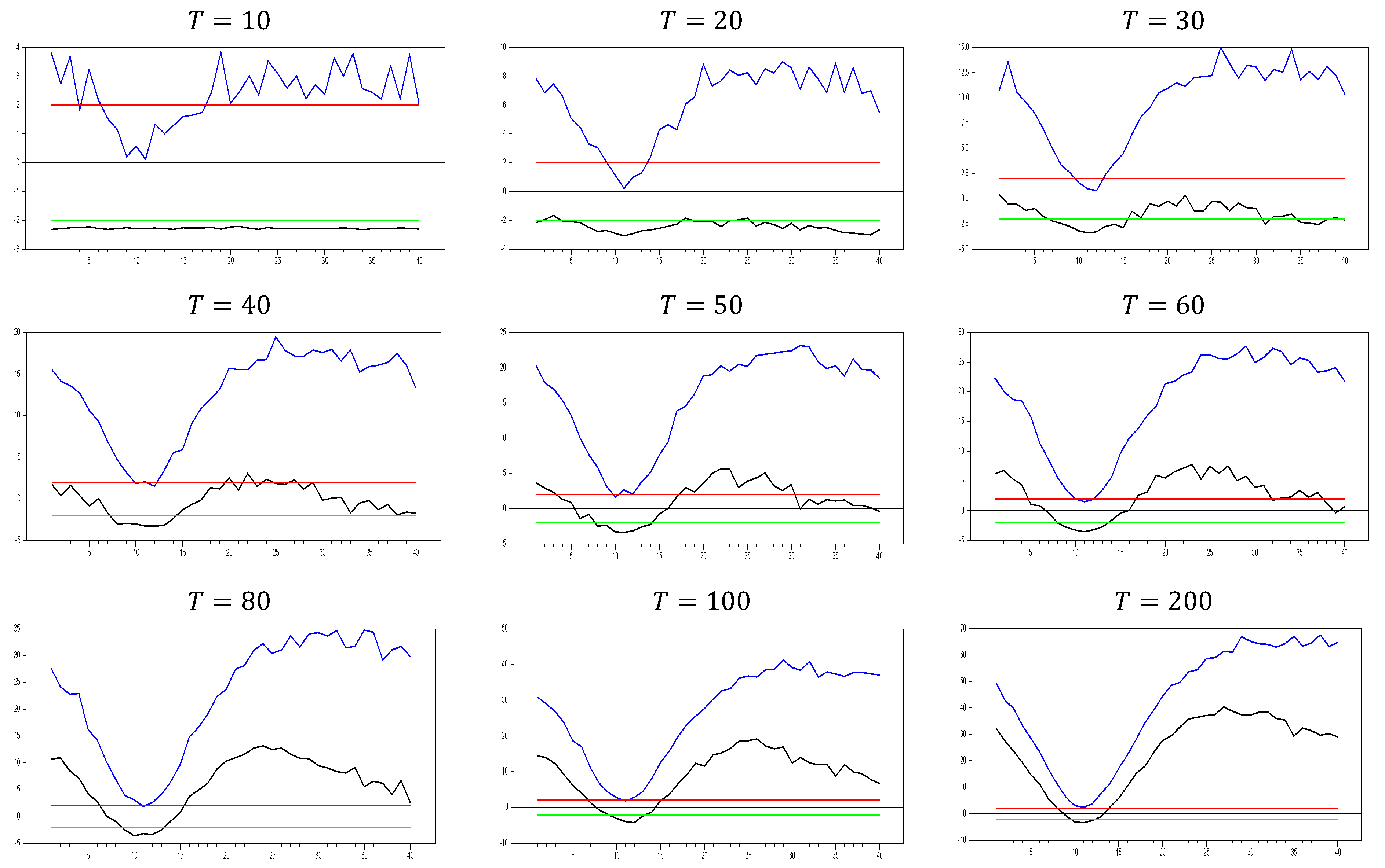
2.2.1. The Behavior of the $C{D}_{LM}$ Without Imposing the CCE Estimator

For the first Monte Carlo study, we use the DGP from Equation (3) without imposing any remedy. The results are shown in Figure 1, Figure 2 and Figure 3.

Figure 1. $C{D}_{LM}$ test results without remedying the CSD data for $N=10$. Note: In the figure, point 10 in the x-axis is 0.0 factor loading and the y-axis shows the $C{D}_{LM}$ test results. The 10 percent significance interval is given as −2.0 and 2.0 as an approximation to −1.96 and 1.96. Moreover for clarification, blue line is the upper bound of the $C{D}_{LM}$ test which is obtained for that specification and the black line is the lowest $C{D}_{LM}$ value obtained for that parameter specification. As for every factor loading we have done simulation study the obtained lower and upper bounds are results from these simulation studies. Green line and red line explained above as −2.0 and 2.0, respectively.

Figure 2. $C{D}_{LM}$ test results without remedying the CSD data for $N=50$. Note: In the figure, point 10 in the x-axis is 0.0 factor loading and the y-axis shows the $C{D}_{LM}$ test results. The 10 percent significance interval is given as −2.0 and 2.0 as an approximation to −1.96 and 1.96.

Figure 3. $C{D}_{LM}$ test results without remedying the CSD data for $N=100$. Note: In the figure, point 10 in the x-axis is 0.0 factor loading and the y-axis shows the $C{D}_{LM}$ test results. The 10 percent significance interval is given as −2.0 and 2.0 as an approximation to −1.96 and 1.96.

As shown in Figure 1, the $C{D}_{LM}$ test effectively captures CSD for $N=10$. The test becomes more sensitive as the $T$ dimension increases. This can be observed in the figures, where for $T=10$, the maximum $C{D}_{LM}$ test value approaches 20.0, while for $T=50$, it increases to around 50. A similar pattern is seen for the minimum values. As $T$ increases, the initially u-shaped $C{D}_{LM}$ test results become skewed, with the tangency points of the curve shortening. This indicates that the $C{D}_{LM}$ test detects CSD for smaller factor loadings as $T$ grows. For $T=200$, the range of test statistics is approximately ($-$0.1, 0.4), indicating almost no CSD, while for $T=10$, the range is wider at (−1.0, 2.4). These results suggest that it is not straightforward to categorize the range (0.0, 0.2) as weak CSD, as some effects are still present when $T$ increases. However, our primary goal is to confirm whether the $C{D}_{LM}$ test is working or not. Based on Figure 1, we conclude that it works well for small $N$ values.

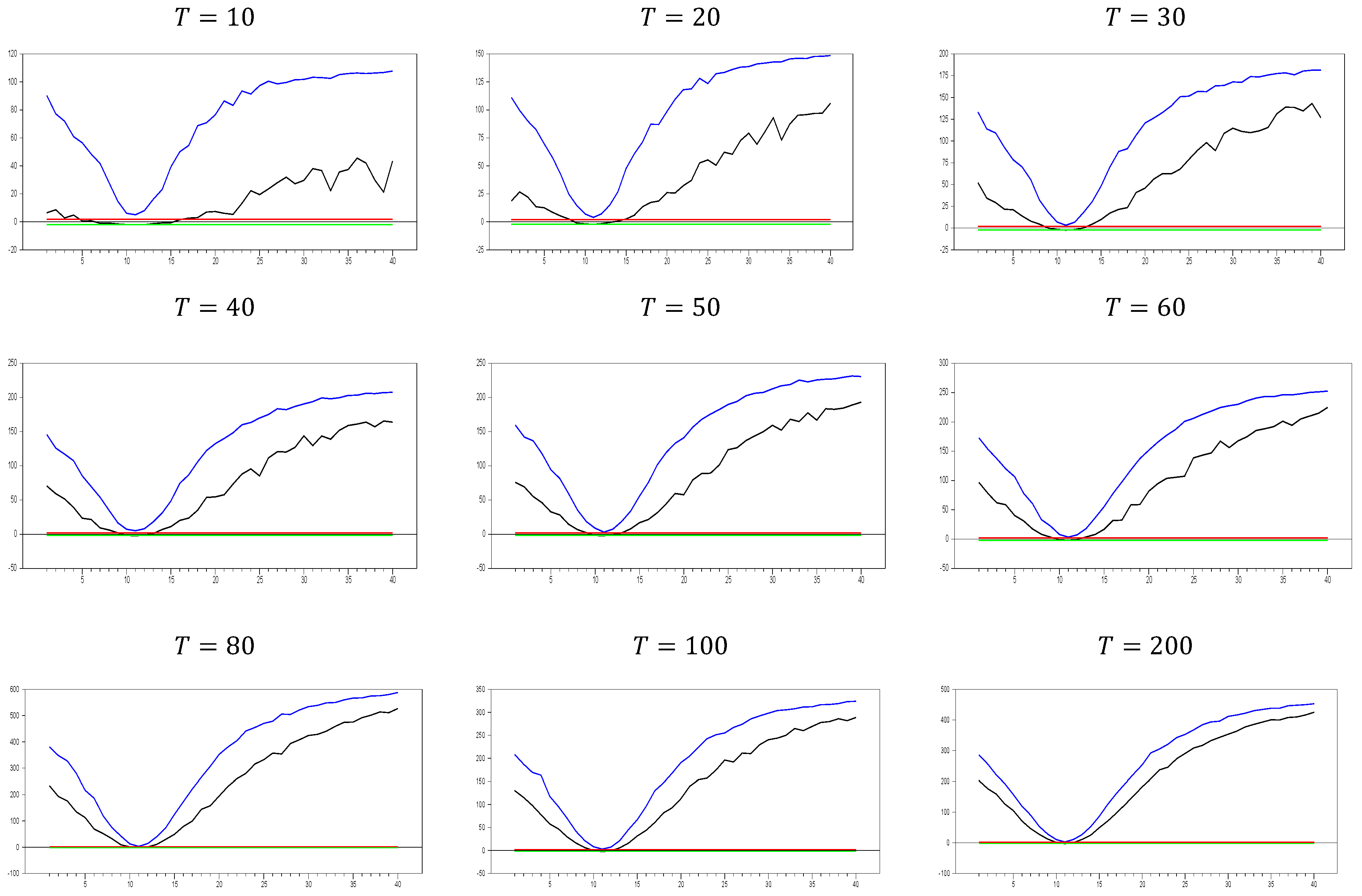
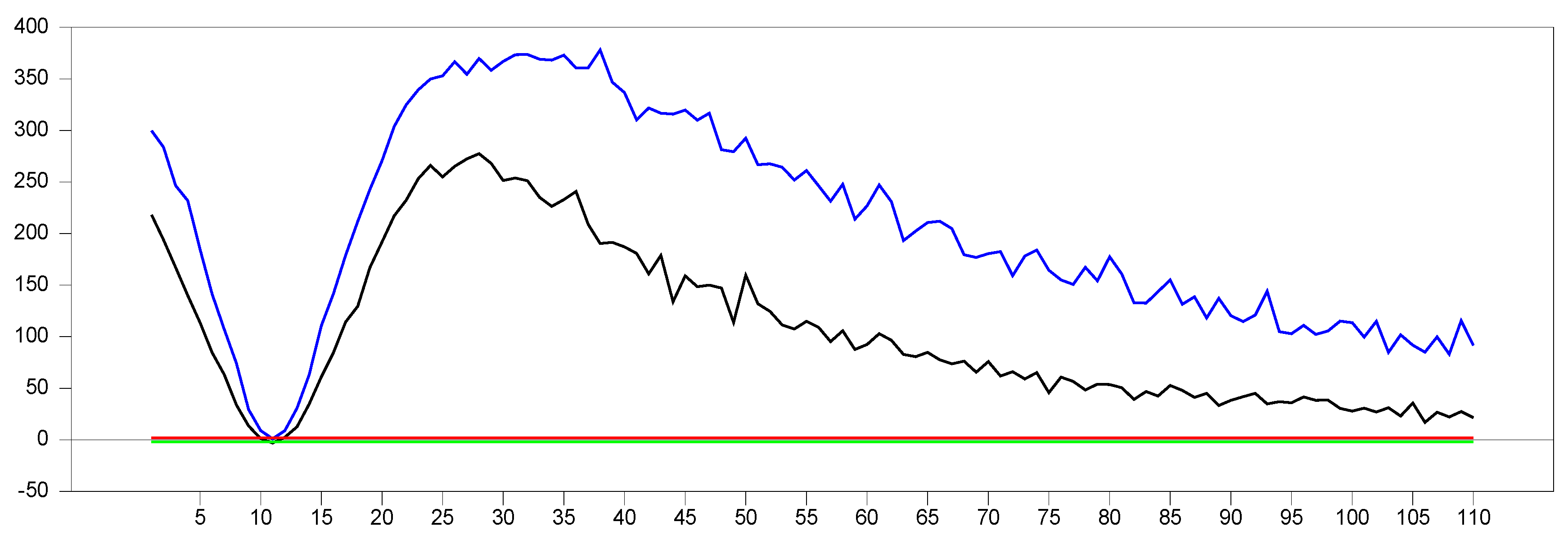
We now move on to test the performance with a larger $N$ value, selecting $N=50$, and the corresponding results are given in Figure 2. As shown in Figure 2, the pattern observed is consistent with that in Figure 1. This confirms that increasing the $N$ dimension does not cause any issues with the $C{D}_{LM}$ test results. Therefore, these simulation results provide evidence of the test’s consistency in small samples. As the $N$ dimension increases, both the maximum and minimum values of the $C{D}_{LM}$ test also increase. For example, with $N=10$ and $T=10$, the maximum $C{D}_{LM}$ test value approaches 20.0, but for $N=50$ and $T=10$, this maximum value rises to approximately 100.0. Similarly, for $N=1$0 and $T=200$, the maximum value is around 50, while for $N=50$ and $T=200$, it increases to 450.0. A similar pattern is observed for the minimum values. Furthermore, as the $N$ dimension increases, the tangency points of the u-shaped figure become shorter, indicating that the $C{D}_{LM}$ test detects CSD for smaller factor loadings.

For $N=10$ and $T=200$, the test produces a range of (−0.1, 0.4), indicating almost no CSD, while for $N=50$ and $T=200$, the range narrows to (0.0, 0.1). Once again, this confirms that it is difficult to classify the range (0.0, 0.2) as weak CSD for all values of $N$ and $T$, as claimed by [8,27]. However, for large values of $N$ and $T$, factor loadings in the range ${\lambda }_i=\left(\mathrm{0.0,0.2}\right)$ can indeed be categorized as weak CSD.

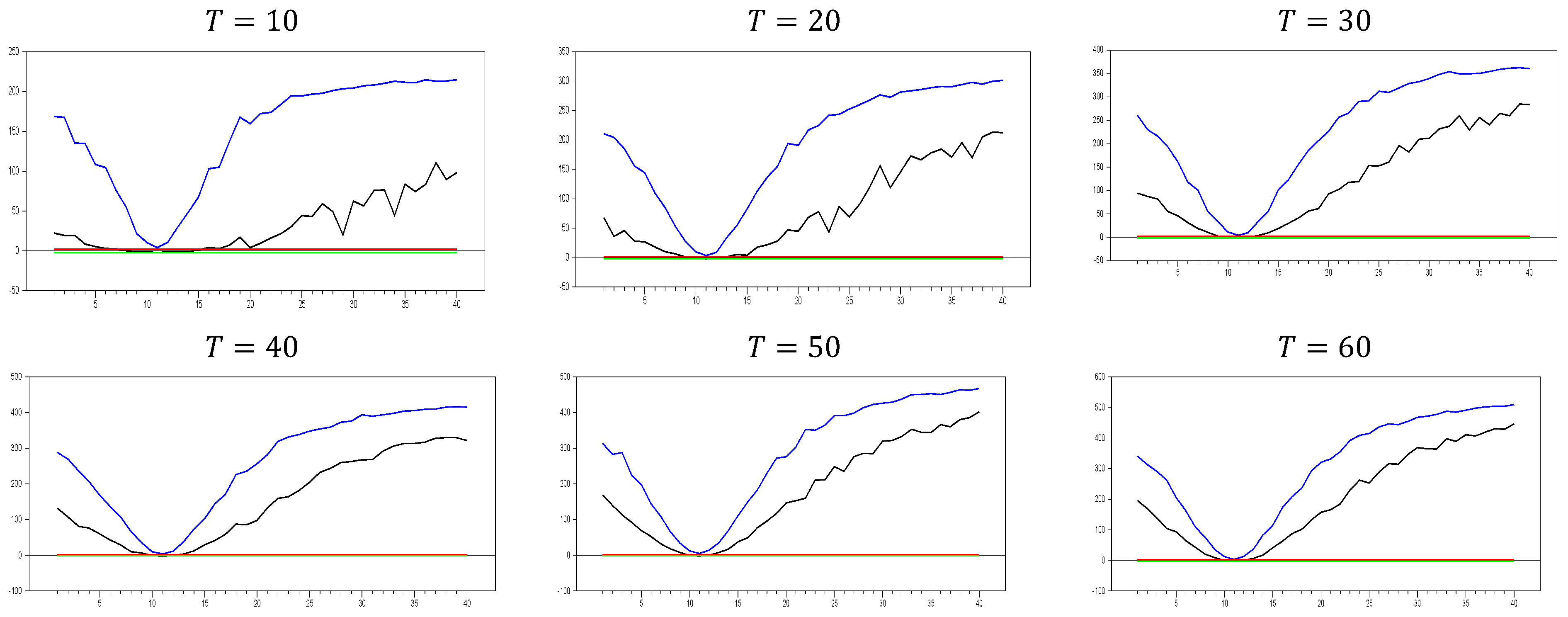
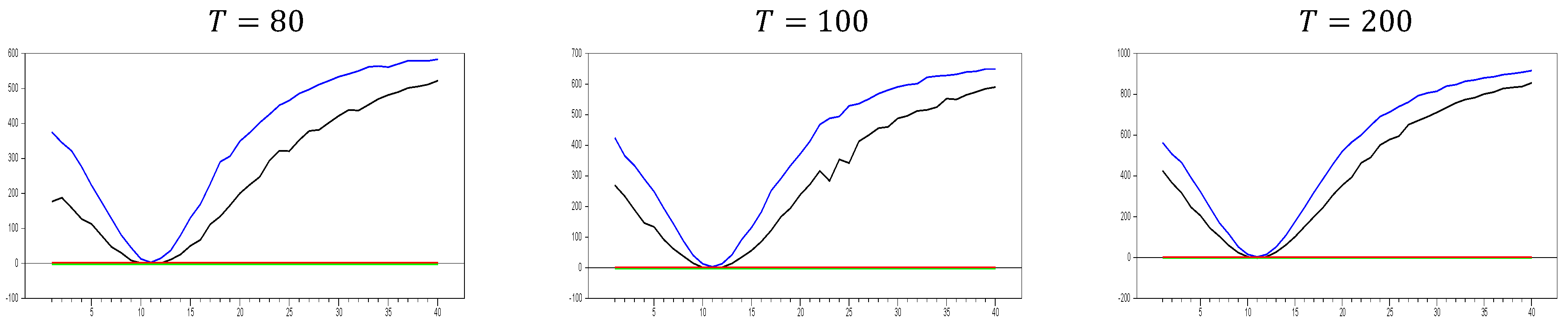
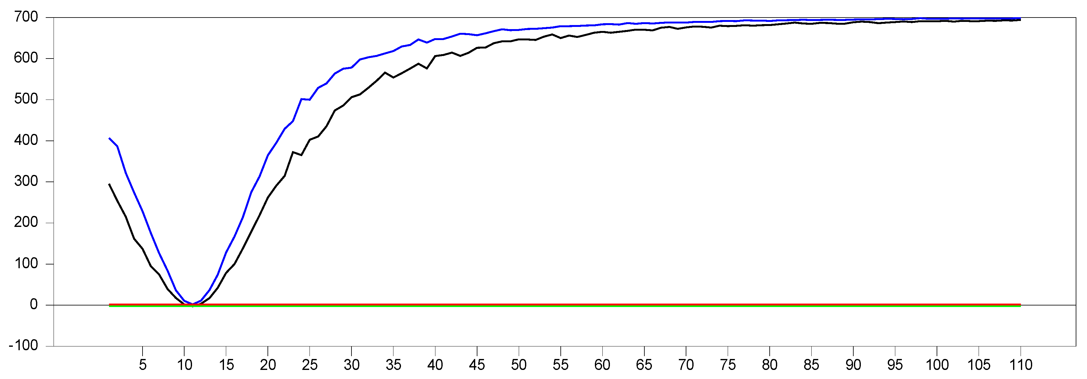
Up until here in Figure 2 and Figure 3, we have deal with $N=50$ and $N=100$ with $T=\{10, 20, 30 40, 50 ,60, 80, 100, 200\}$. In order to see the large sample features, we performed simulations for $N=200$ and $T=1000$. Figure 4 shows the behavior of the $C{D}_{LM}$ test in large samples. Figure 4 confirms the expected pattern of Figure 1, Figure 2 and Figure 3. All the explanations for the comparison of Figure 1, Figure 2 and Figure 3 are valid. Hence, these simulation results provide evidence of the consistency of the test for catching CSD in small samples.

Figure 4. $C{D}_{LM}$ test results without remedying the CSD data for $N=200$ and $T=1000$.

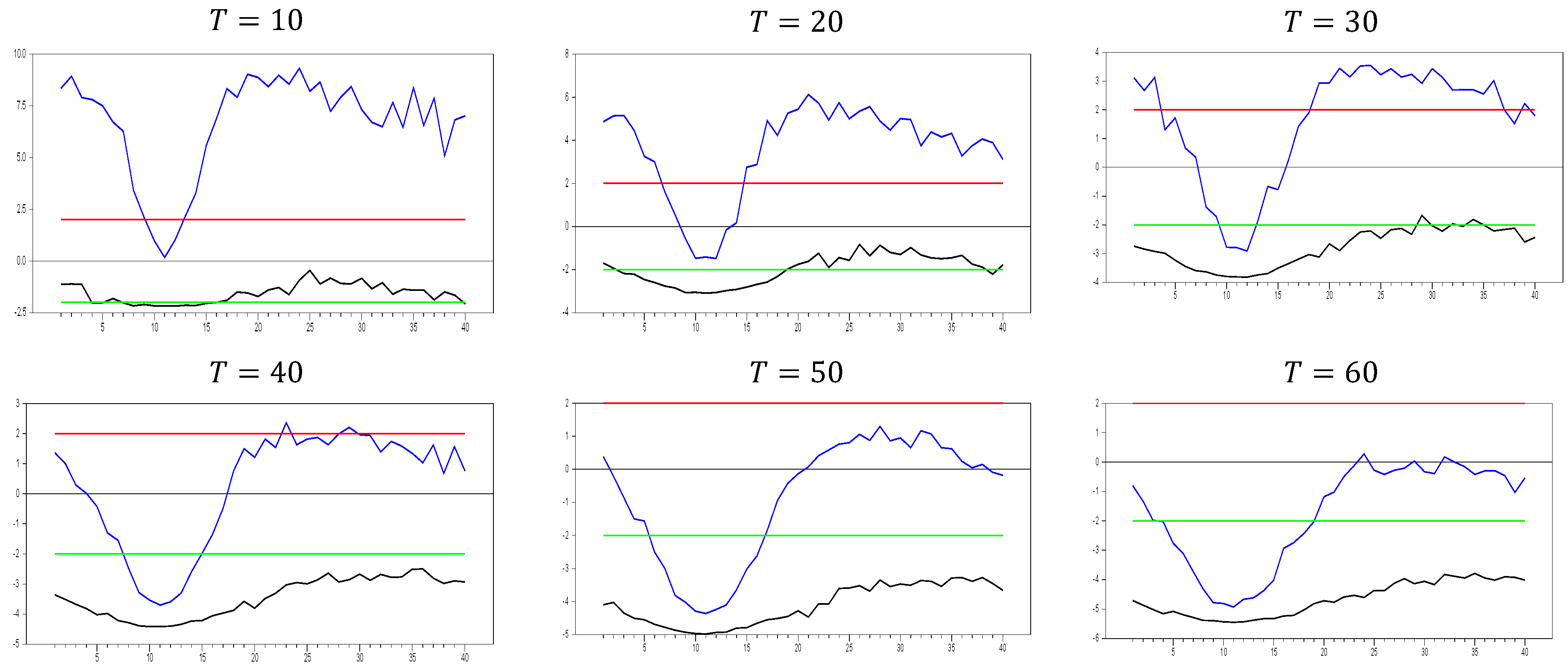
2.2.2. The Behavior of the $C{D}_{LM}$ with Imposing the Factor Variable

We now investigate the consistency of the $C{D}_{LM}$ test by imposing a factor variable into the testing process, which induces CSD in the DGP. If the $C{D}_{LM}$ test is working correctly, the inclusion of the factor variable should eliminate the CSD, and the $C{D}_{LM}$ test should indicate no remaining CSD. The resulting $C{D}_{LM}$ values will fall between the z-test thresholds of −2.0 and 2.0, as shown in the graphics. The first results are given in Figure 5 for $N=10$.

Figure 5. $C{D}_{LM}$ test results with remedying the CSD by the original factor for $N=10$. Note: In the figure, point 10 in the x-axis is 0.0 factor loading and the y-axis shows the $C{D}_{LM}$ test results. The 10 percent significance interval is given as −2.0 and 2.0 as an approximation to −1.96 and 1.96.

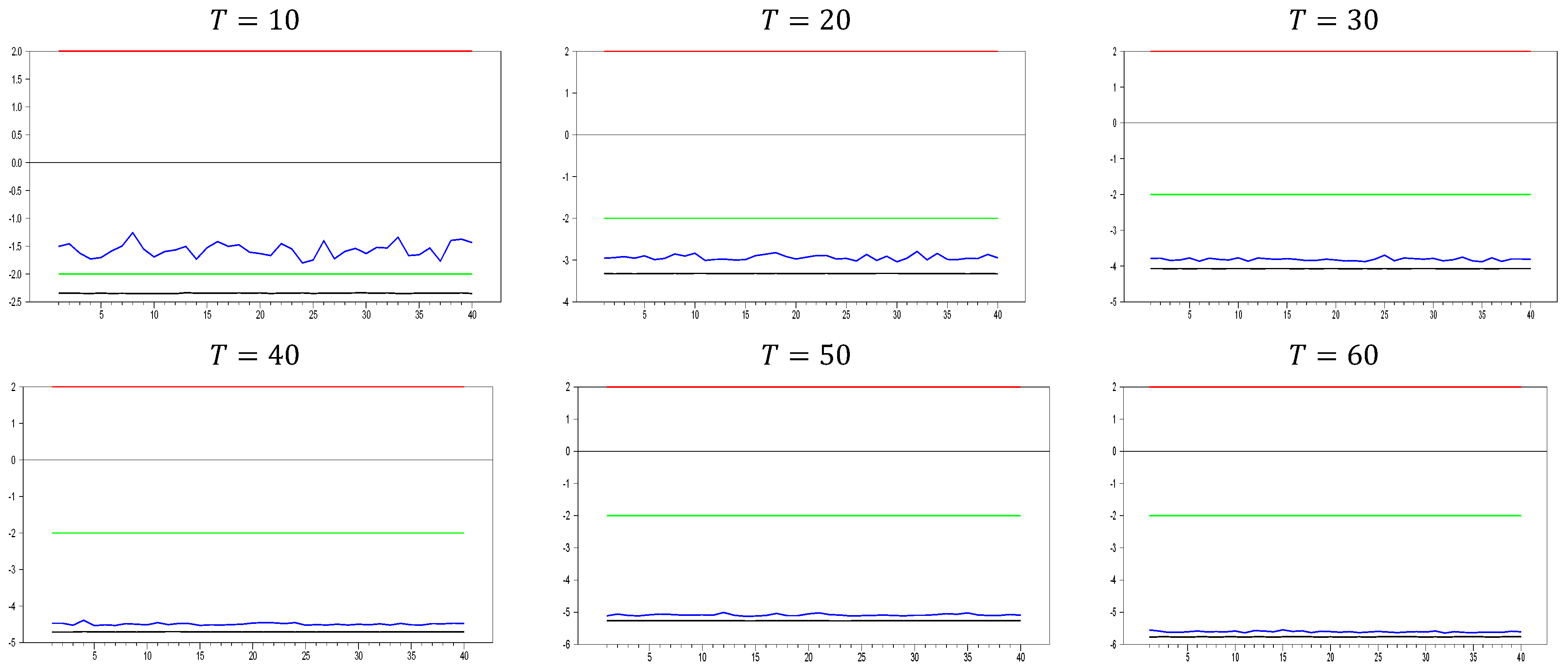
From Figure 5, we observe that the calculated minimum and maximum values fall within the 10% significance level of the z-test, confirming that the $C{D}_{LM}$ test successfully captures the CSD imposed in the DGP of Equation (3). This result meets our expectations and provides a benchmark for evaluating proxies used to remedy CSD. A valid proxy should follow this pattern for small $N$ and $T$ dimensions. If the test shows no CSD for any factor loading, the proxy can be considered an efficient factor variable. In Figure 5, we can see how increasing the $T$ dimension affects the results. The test statistics range between approximately −2.0 and 7.0 for $T=10$, and between −3.0 and 4.0 for $T=200$. As $T$ increases, the band of calculated test statistics narrows and shifts downward, with the maximum values decreasing more significantly than the minimum values. This suggests that while the original factor effectively remedies CSD, it still has some limitations in handling very small probabilities. To better understand the $C{D}_{LM}$ test’s behavior, it would be useful to analyze the results with a larger $N$ dimension.

From Figure 6, we can observe that for $N=50$ and $T=10$, the calculated $C{D}_{LM}$ test statistics range between approximately −1.5 and 15.0, compared to a range of −2.0 to 7.0 for $N=10$ and $T=10$. As $N$ increases, the band of the $C{D}_{LM}$ test statistics shifts upward and widens, with the maximum values increasing more than the minimum values. When $N=50$ and $T=200$, the band narrows to a range of −2.0 to 4.0, whereas for $N=10$ and $T=200$, the range is approximately −3.0 to 4.0. This narrowing of the band as both $N$ and $T$ increase suggests that the original factor more effectively remedies CSD in the DGP. These simulations highlight the power of the $C{D}_{LM}$ test, which proves to be highly effective in detecting CSD based on the test results. The second set of simulations further demonstrates the effectiveness of the method in remedying CSD, building on the first simulation’s results. Therefore, we can conclude that both simulations confirm the power of the $C{D}_{LM}$ test and the method used to remedy CSD.

Figure 6. $C{D}_{LM}$ test results with remedying the CSD by the original factor for $N=50$. Note: In the figure, point 10 in the x-axis is 0.0 factor loading and the y-axis shows the $C{D}_{LM}$ test results. The 10 percent significance interval is given as −2.0 and 2.0 as an approximation to −1.96 and 1.96.

To explore this further, we now examine the impact of increasing the $N$ dimension in Figure 7. In Figure 7, a new phenomenon emerges. When the factor loadings are low, the original factor remedies CSD more effectively than at higher factor loadings. This behavior may also appear in approximation methods like the CCE estimator.

Figure 7. $C{D}_{LM}$ test results with remedying the CSD by the original factor for $N=100$. Note: In the figure, point 10 in the x-axis is 0.0 factor loading and the y-axis shows the $C{D}_{LM}$ test results. The 10 percent significance interval is given as −2.0 and 2.0 as an approximation to −1.96 and 1.96.

Up until here in Figure 5, Figure 6 and Figure 7, we have deal with $N=10$, $N=50$ and $N=100$ with $T=\{10, 20, 30 40, 50 ,60, 80, 100, 200\}$. To explore the behavior in larger samples, we conducted a simulation with $N=200$ and $T=1000$. Figure 8 illustrates how the $C{D}_{LM}$ test performs in remedying CSD using the original factor in these large-sample settings.

Figure 8. $C{D}_{LM}$ test results with remedying the CSD by the original factor for $N=200$ and $T=1000$.

We now have solid benchmark simulations to assess whether the proxy variables are effective. The results from the first simulation help us evaluate whether the proxy can remedy part of CSD. The second set of simulations further demonstrates the efficiency of the proposed method in addressing CSD.

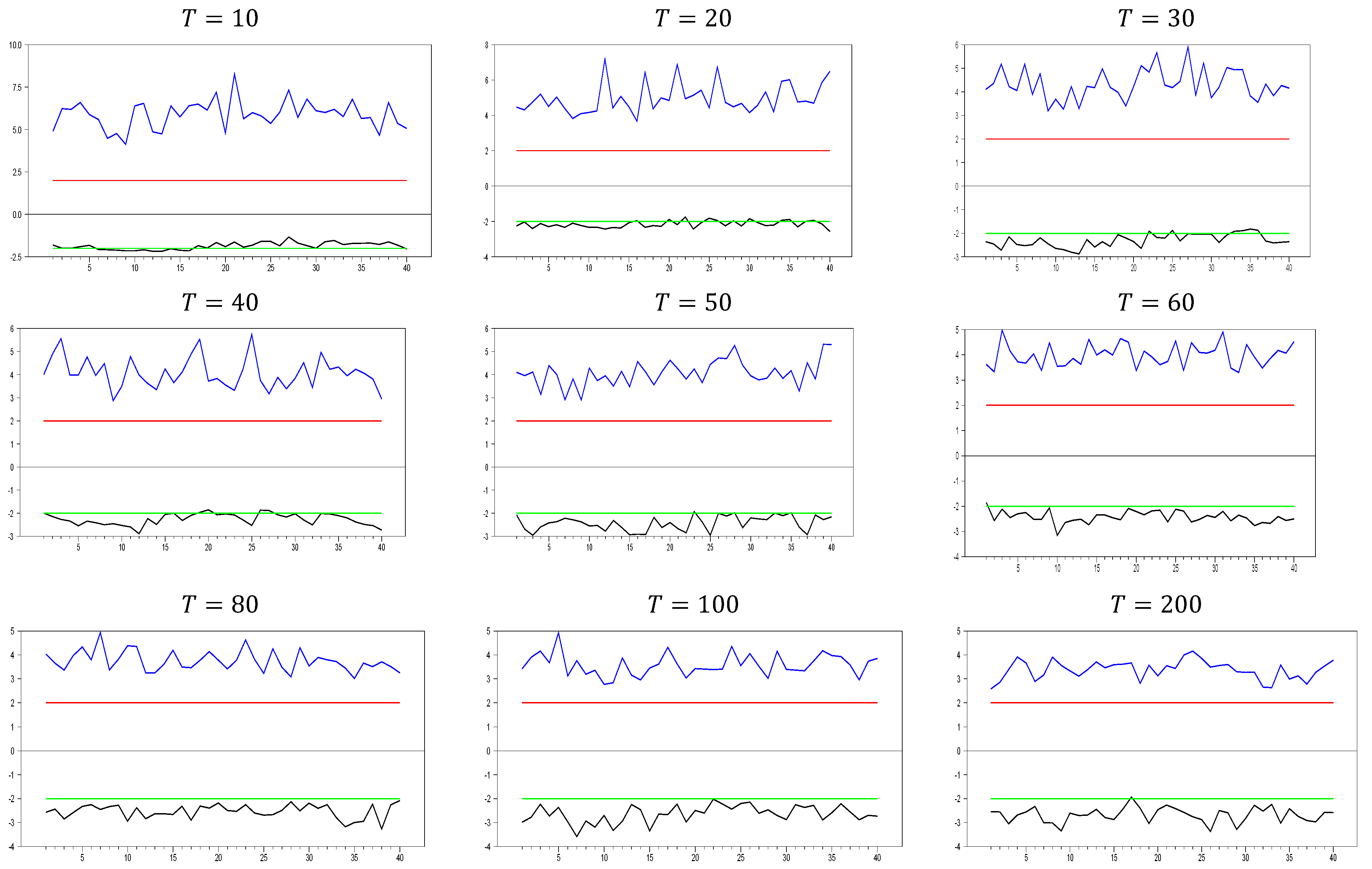
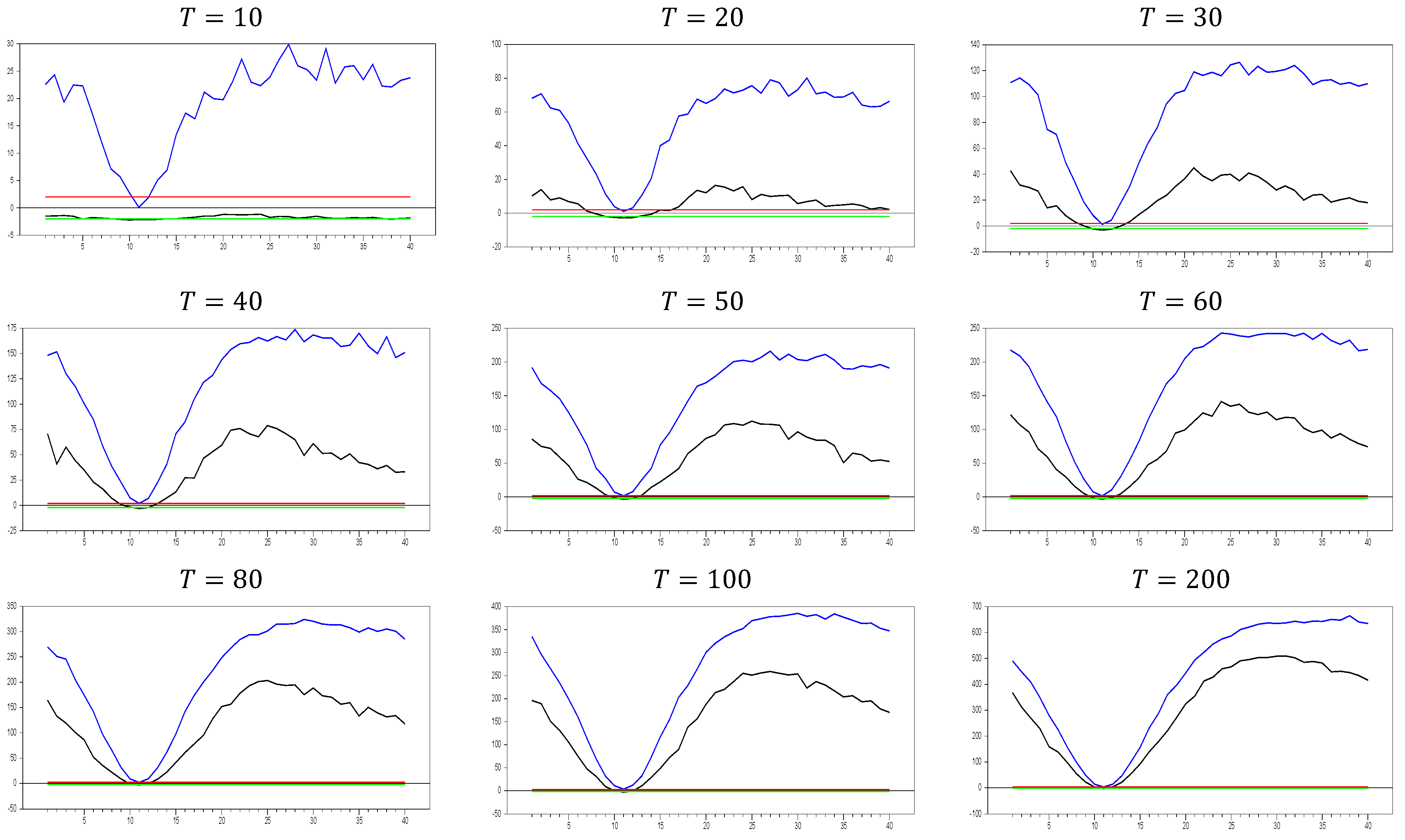
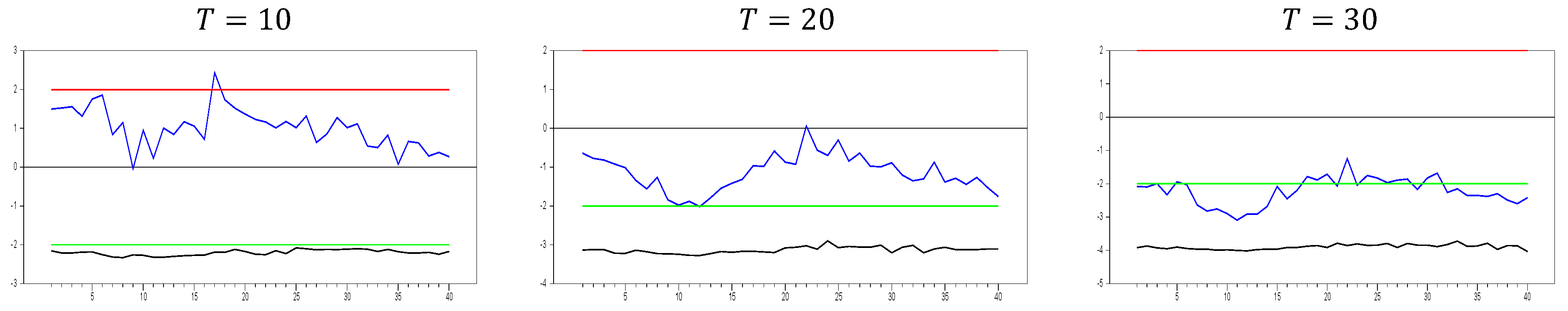
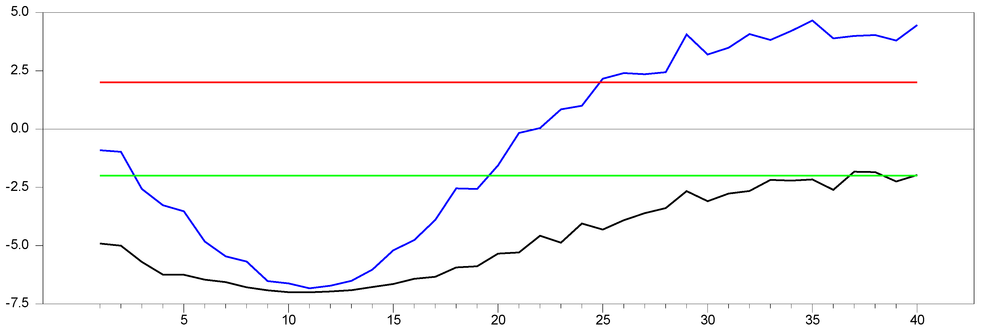
2.2.3. The Behavior of the $C{D}_{LM}$ with Imposing the CCE Estimator

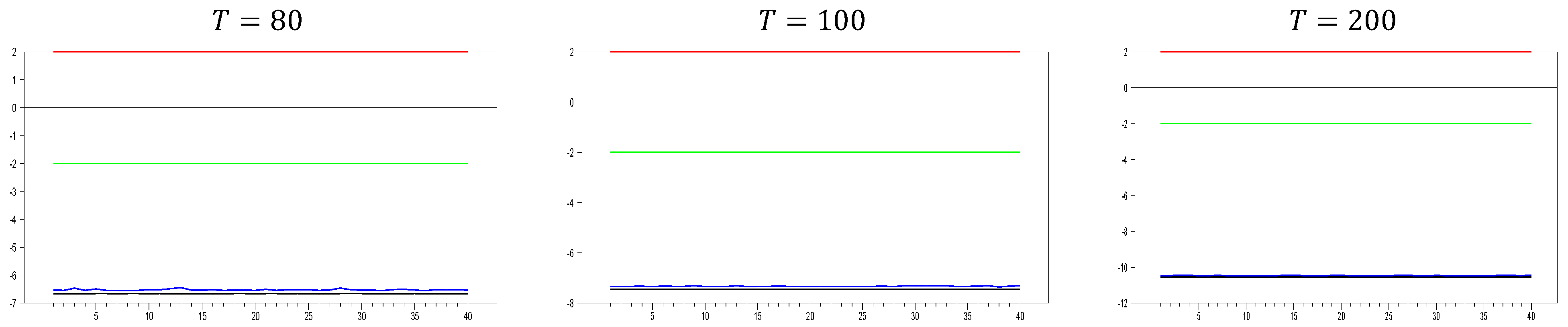
In light of these arguments, we can assess performances of the CCE estimator proposed by [8,27]. In Figure 9, we observe some unexpected results for what would typically be considered a good proxy. However, only for $N=10$ and $T=10$ do we see the expected results for a proxy that remedies CSD, as indicated by simulations 1 and 2. The computed $C{D}_{LM}$ values range between approximately −2.4 and −1.5, demonstrating that the CCE estimator effectively remedies CSD. Additionally, for $T=20$, the computed values quickly move out of the CSD rejection region, and the band between the minimum and maximum $C{D}_{LM}$ values narrows as the $T$ dimension increases. By $T=200$, the minimum and maximum values of the $C{D}_{LM}$ test are approximately $-$10.25 and −10.15, respectively. Now, we can further explore the effects of increasing the $N$ dimension.

Figure 9. $C{D}_{LM}$ test results with remedying the CSD by the CCE method for $N=10.$ Note: In the figure, point 10 in the x-axis is 0.0 factor loading and the y-axis shows the $C{D}_{LM}$ test results. The 10 percent significance interval is given as −2.0 and 2.0 as an approximation to −1.96 and 1.96.

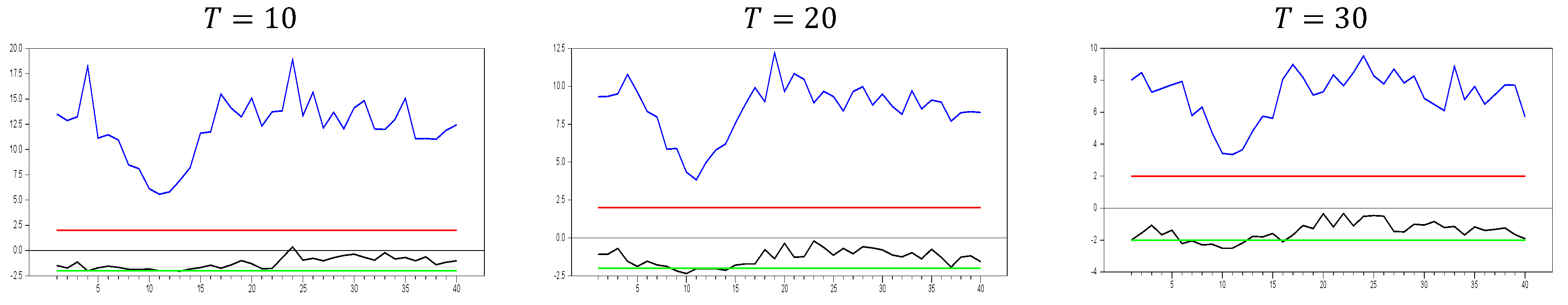
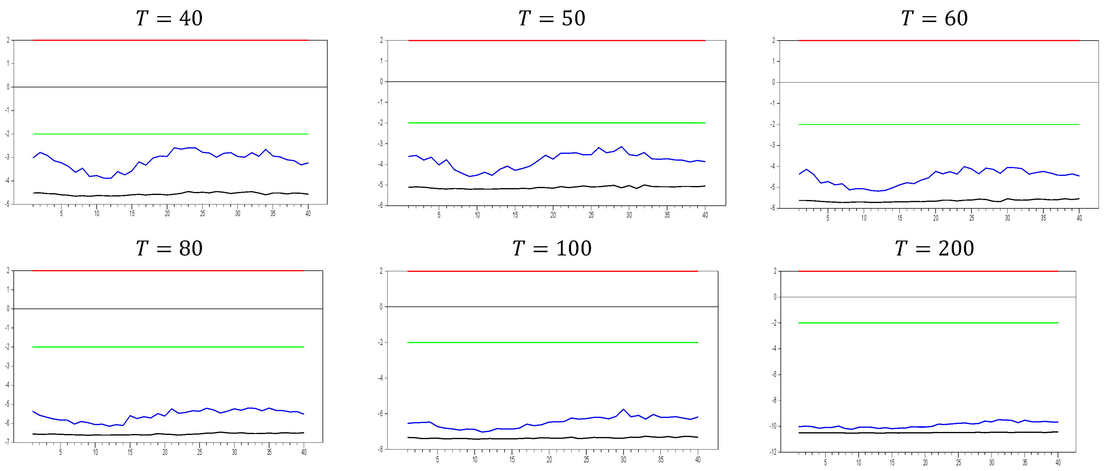
In Figure 10, we observe that only for $N=20$ and $T=10$ we obtain the expected results for a good proxy that remedies CSD, as indicated by simulations 1 and 2. The computed $C{D}_{LM}$ values range between approximately −2.2 and −1.4, confirming that the CCE estimator effectively remedies CSD. However, as the $N$ dimension increases, the band between the minimum and maximum $C{D}_{LM}$ values narrows. For $N=50$ and $N=10$, the minimum and maximum $C{D}_{LM}$ values for $T=200$ are approximately $\left(-10.25,-10.15\right)$ and $\left(-10.05,-10.10\right)$, respectively. These results show that increasing $T$ reduces the $C{D}_{LM}$ test values and narrows the band, while increasing $N$ further narrows the range. The key finding from these simulations, in line with simulations 1 and 2, is that the CCE estimator remedies CSD most effectively when $T$ is small. However, as $T$ increases, the proxies $\mathsf{\Delta }{\overline{y}}_t$ and ${\overline{y}}_{t-1}$ correct the factor’s effect in the residual term but introduce additional CSD in the opposite direction. These simulations focus solely on CSD, so we cannot yet determine how they impact bias reduction in the ${\beta }_i$ parameter in Equation (3). Nonetheless, there remains scope for developing a better estimator for addressing CSD in panel unit root testing, in line with the approaches of [8,27]. Before further investigating this, it is beneficial to examine the effects of increasing both $N$ and $T$ dimensions.

Figure 10. $C{D}_{LM}$ test results with remedying the CSD by the CCE method for $N=50$. Note: In the figure, point 10 in the x-axis is 0.0 factor loading and the y-axis shows the $C{D}_{LM}$ test results. The 10 percent significance interval is given as −2.0 and 2.0 as an approximation to −1.96 and 1.96.

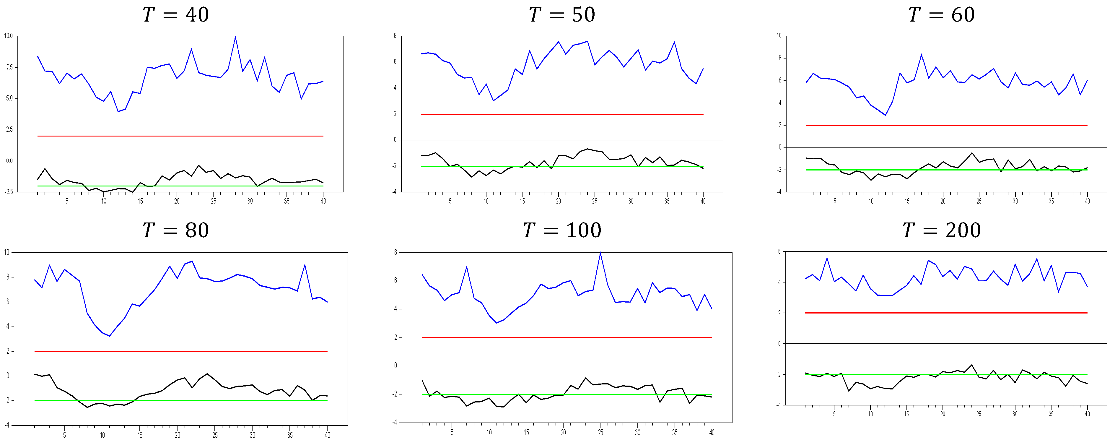
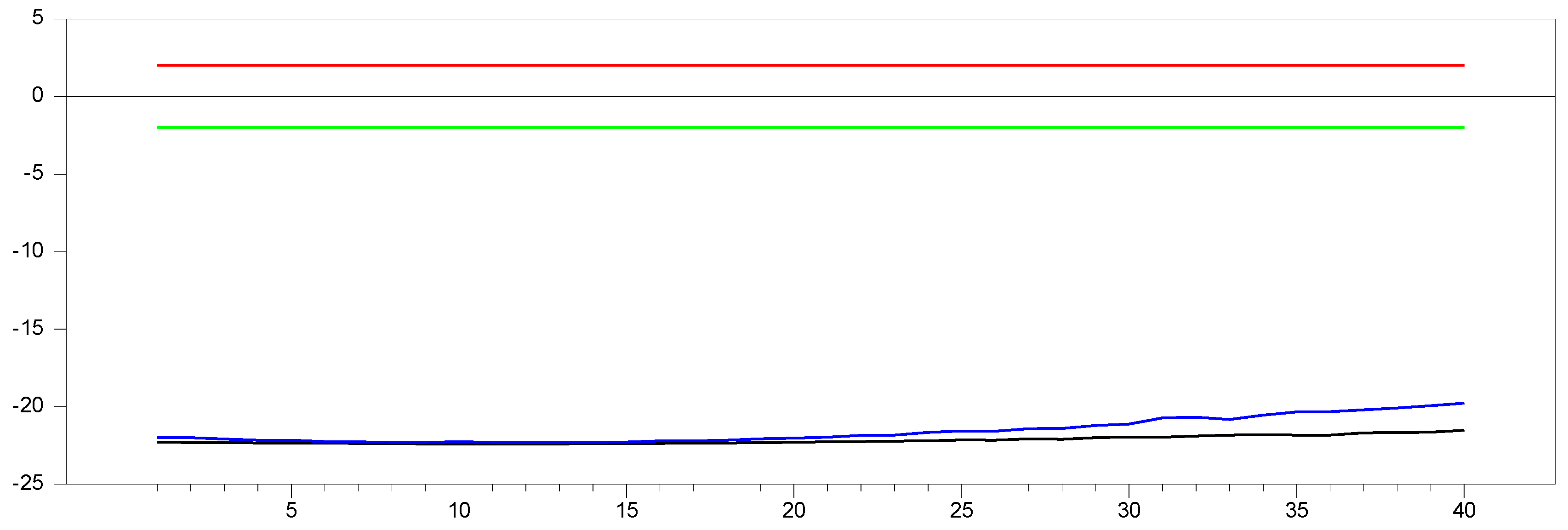
In Figure 11, we observe that the results are similar to those in Figure 9 and Figure 10. The only difference is that for $N=100$ and $T=200$, no band appears, and the minimum and maximum values are fixed at 10.0. This indicates that the bands in Figure 11 are narrower than those in Figure 9 and Figure 10. To further explore the behavior in large samples, we conducted a simulation for $N=200$ and $T=1000$.

Figure 11. $C{D}_{LM}$ test results with remedying the CSD by the CCE method for $N=100$. Note: In the figure, point 10 in the x-axis is 0.0 factor loading and the y-axis shows the $C{D}_{LM}$ test results. The 10 percent significance interval is given as −2.0 and 2.0 as an approximation to −1.96 and 1.96.

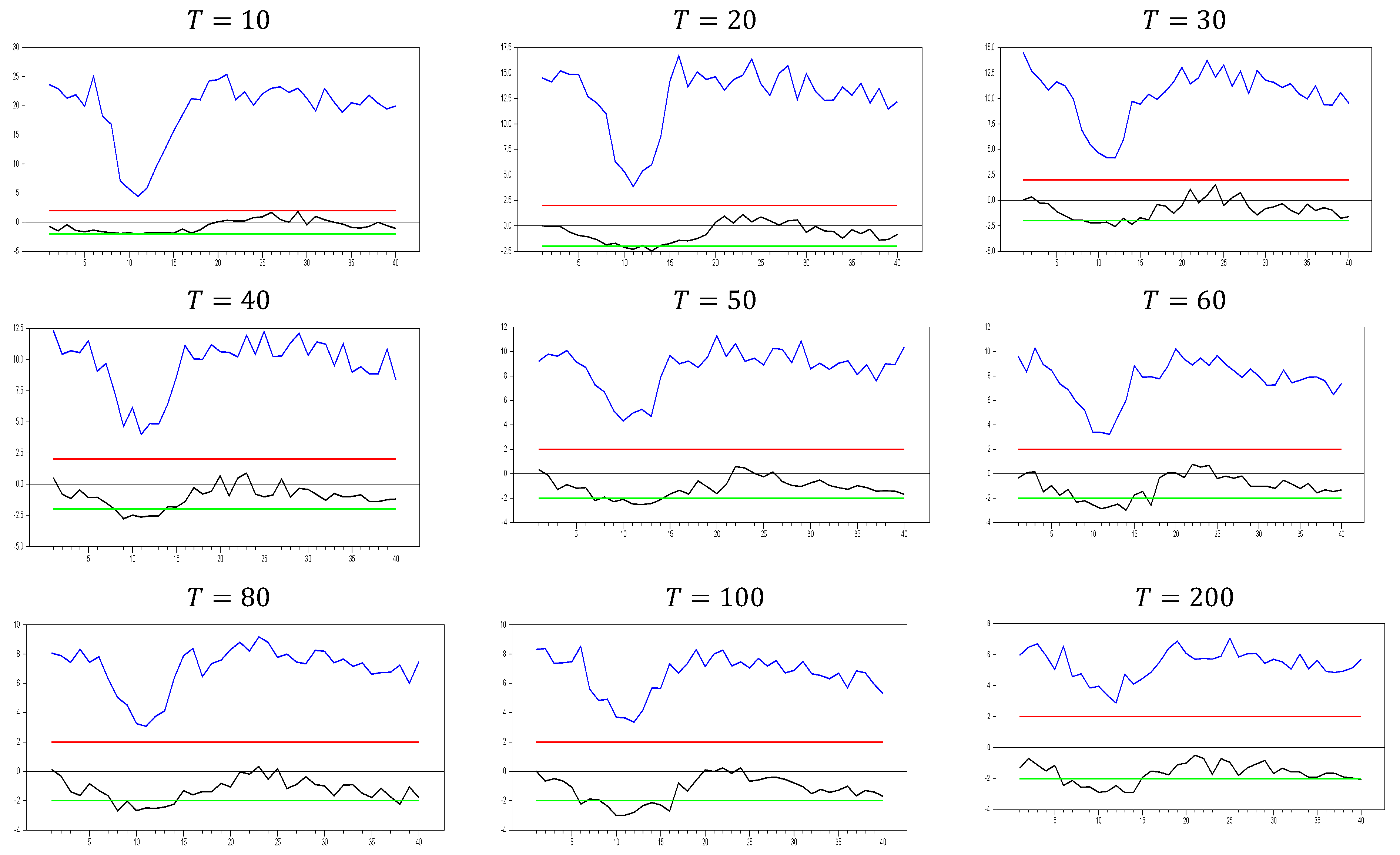
Figure 12 illustrates how the $C{D}_{LM}$ test performs when remedying CSD using the CCE estimator proposed by [27] in large samples. In Figure 12, we observe that as the $T$ dimension increases, the $C{D}_{LM}$ test values reach 22.0. Additionally, increasing both the $T$ and $N$ dimensions together eliminate the band between the minimum and maximum values of the $C{D}_{LM}$ test.

Figure 12. $C{D}_{LM}$ test results with remedying the CSD by CCE for $N=200$ and $T=1000$.

2.3. The Refinement of the Common Correlated Estimator by Using the $C{D}_{LM}$ Test Results

In light of these findings, we now can investigate for a more efficient estimator for remedying CSD in small samples.

$$∆y_{it}=b_i{y}_{i,t-1}+c_i{\overline{y}}_{t-1}+d_i∆{\overline{y}}_t+e_{it}$$

(11)

Proposition 1.

$d_i\Delta {\overline{y}}_t$ and  $c_i{\overline{y}}_{t-1}$ proxies can be expressed by  $c_i{\overline{y}}_t$.

Proof. 

$$d_i\mathsf{\Delta }{\overline{y}}_t+c_i{\overline{y}}_{t-1}=c_i{\overline{y}}_t$$

(12)

$\mathsf{\Delta }{\overline{y}}_t$ with some algebra can show that

$$d_i{\overline{y}}_t-d_i{\overline{y}}_{t-1}+c_i{\overline{y}}_{t-1}=c_i{\overline{y}}_t$$

(13)

$$d_i{\overline{y}}_t-\left(d_i-c_i\right){\overline{y}}_{t-1}=c_i{\overline{y}}_t$$

(14)

where ${\overline{y}}_{t-1}=N^{-1}{\sum }_{i=1}^N{y}_{i,t-1}$ and $t-1=s$ is taken:

$${\overline{y}}_{t-1}=N^{-1}\sum _{i=1}^N{y}_{i,s}$$

(15)

Hence, we can write

$$N^{-1}\left[\sum _{i=1}^N{y}_{i,s}+\left(y_{i,n}+y_{i,0}\right)\right]$$

(16)

$$N^{-1}\sum _{i=1}^N{y}_{i,s}={\overline{y}}_t$$

(17)

Now, we can re-write Equation (12),

$$d_i{\overline{y}}_t-d_i{\overline{y}}_t+c_i{\overline{y}}_t+2\left(y_{i,n}+y_{i,0}\right)/n=c_i{\overline{y}}_t$$

(18)

With some algebra,

$$c_i{\overline{y}}_t+2\left(y_{i,n}+y_{i,0}\right)/n=c_i{\overline{y}}_t$$

(19)

Showing that

$$\left(y_{i,n}+y_{i,0}\right)⟶O_p\left(1/\sqrt{N}\right)$$

(20)

we prove that

$$d_i\mathsf{\Delta }{\overline{y}}_t+c_i{\overline{y}}_{t-1}=c_i{\overline{y}}_t$$

□

Using this variable, $c_i{\overline{y}}_t$, may provide a more effective proxy factor to address cross-sectional dependency compared to [27]’s CCE estimator. In the CCE estimator, we use two variables to proxy the factor; now, we have only one parameter to estimate, which may increase the efficiency.

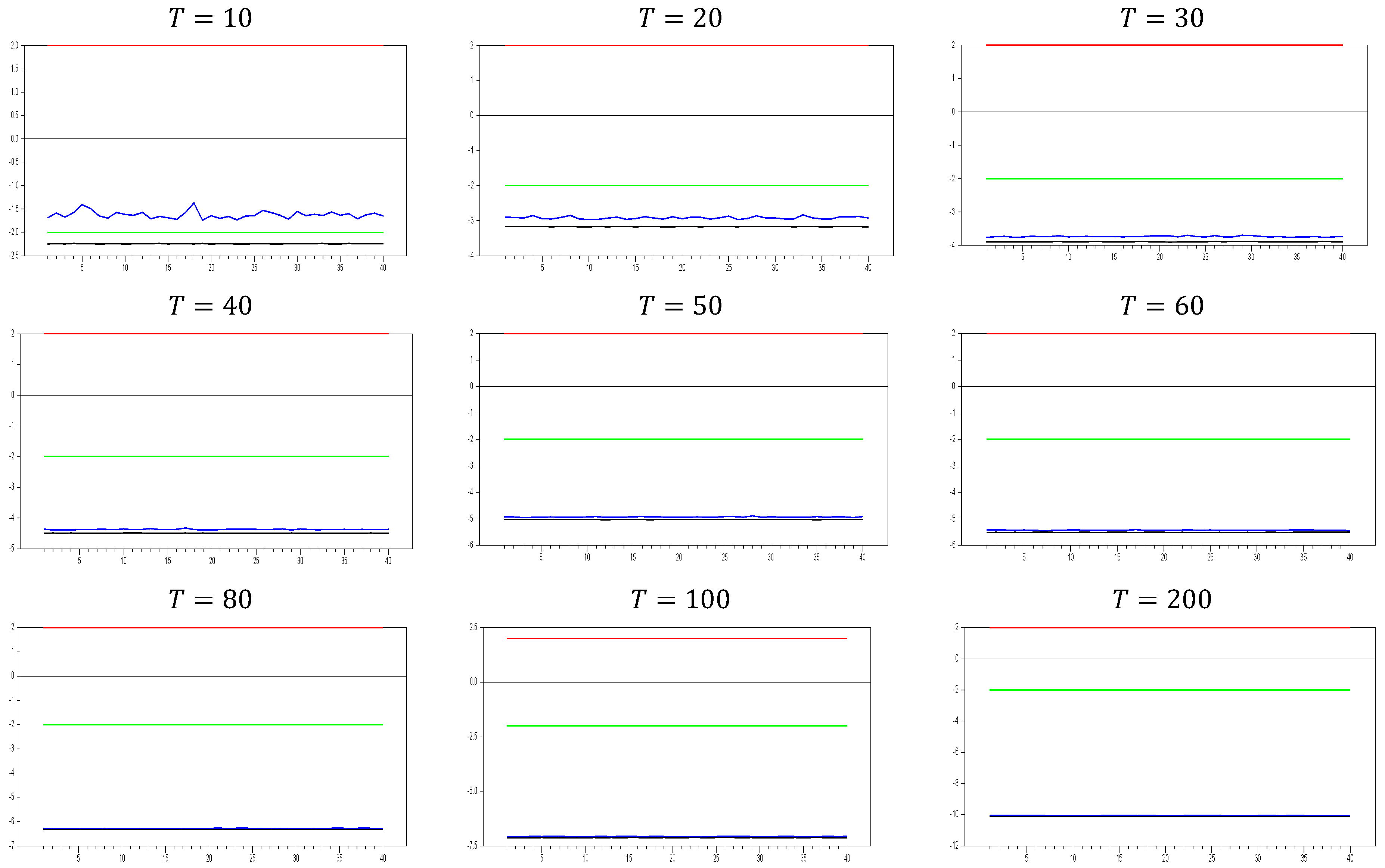
Figure 13 clearly demonstrates that, for small $T$ values, the newly proposed estimator or proxy closely mimics the original factor variable. Specifically, for $N=10$ and $T=\left\{\mathrm{10,20,30}\right\}$, the new proxy closely replicates the original factor variable based on the $C{D}_{LM}$ test results shown in Figure 5. However, as the $T$ dimension increases, both the minimum and maximum $C{D}_{LM}$ test values rise, and the band widens. By $T=80$, the $C{D}_{LM}$ test results for the proxy estimator indicate that it no longer provides an effective remedy. To further examine the effect of increasing the $N$ dimension, we performed a simulation for $N=50$. The results are shown in Figure 14. Figure 14 shows that the effectiveness of the newly proposed estimator in remedying CSD diminishes as the $N$ dimension increases. Thus, we can conclude that this proxy is only effective for very small $T$ dimensions.

Figure 13. $C{D}_{LM}$ test results with remedying the CSD by the ${\overline{y}}_t$ variable only for $N=10$. Note: In the figure, point 10 in the x-axis is 0.0 factor loading and the y-axis shows the $C{D}_{LM}$ test results. The 10 percent significance interval is given as −2.0 and 2.0 as an approximation to −1.96 and 1.96.

Figure 14. $C{D}_{LM}$ test results with remedying the CSD by the ${\overline{y}}_t$ variable only for $N=50$. Note: In the figure, point 10 in the x-axis is 0.0 factor loading and the y-axis shows the $C{D}_{LM}$ test results. The 10 percent significance interval is given as −2.0 and 2.0 as an approximation to −1.96 and 1.96.

To further examine the impact of increasing the $N$ dimension, we conducted a simulation for $N=100$. The results are presented in Figure 15. Fortunately, as seen in Figure 15, the $C{D}_{LM}$ test results for $N=100$ and $T=200$ show that the test values converge to 1000.0, while the new estimator’s $C{D}_{LM}$ test values converge to 600.0. This indicates that the new estimator remedies part of the CSD, but a significant portion of the induced CSD still remains, leading to biased estimates. Additionally, the $C{D}_{LM}$ test values start to decrease around a factor loading of $\lambda =1.0$, opposite to the trend in Figure 15. Therefore, it may be useful to examine the behavior of the $C{D}_{LM}$ test for higher factor loadings.

Figure 15. $C{D}_{LM}$ test results with remedying the CSD by the ${\overline{y}}_t$ variable only for $N=100$. Note: In the figure, point 10 in the x-axis is 0.0 factor loading and the y-axis shows the $C{D}_{LM}$ test results. The 10 percent significance interval is given as −2.0 and 2.0 as an approximation to −1.96 and 1.96.

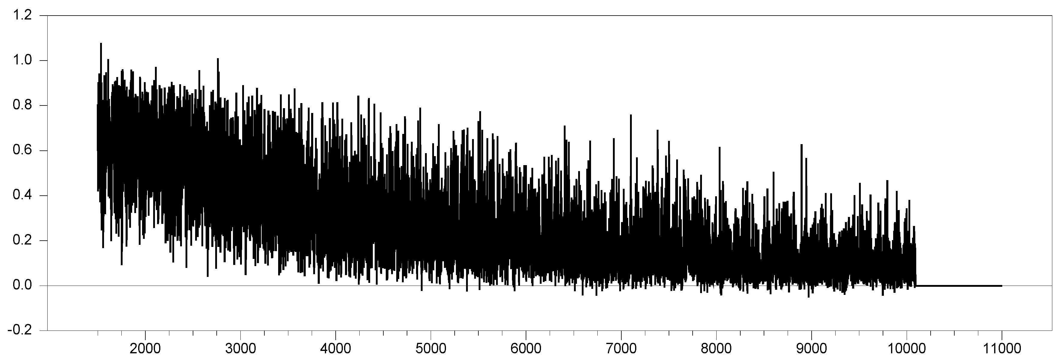
Figure 16 presents the simulation results for $N=100$ and $T=100$ with factor loadings ranging from ${\lambda }_i=\left[-\mathrm{1.0,10.0}\right]$ in 0.1 increments. As the factor loadings increase, the new proxy ${\overline{y}}_t$ adjusts within the range of ${\lambda }_i=\left[-\mathrm{1.0,10.0}\right]$. 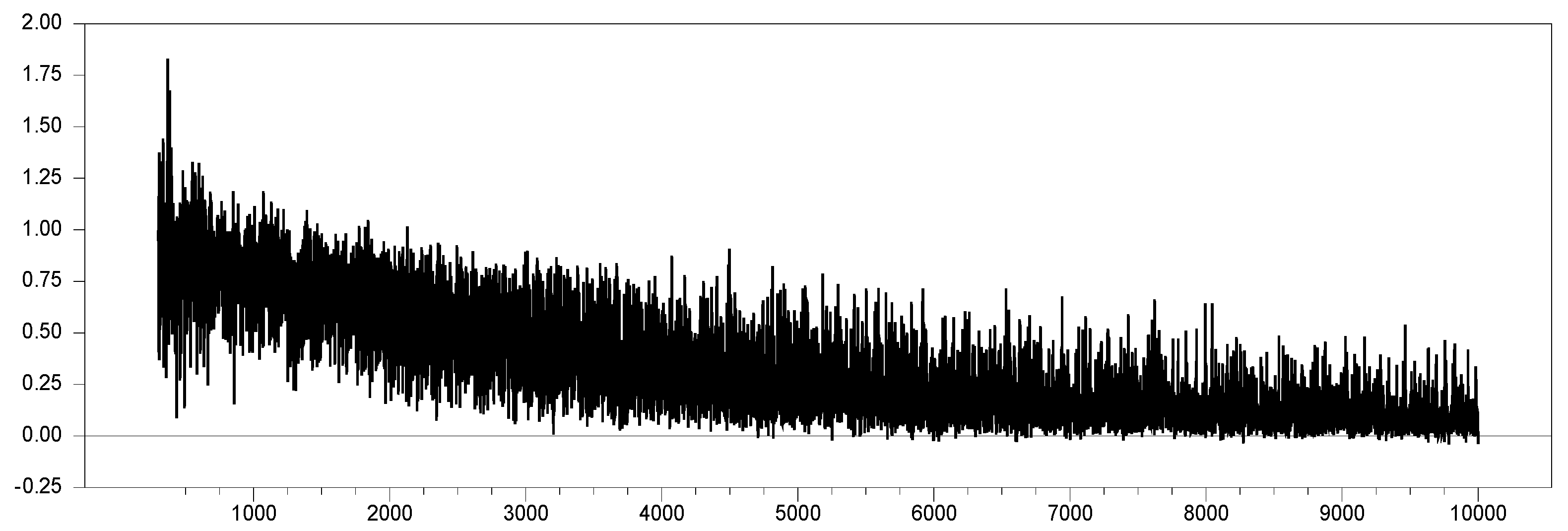To better understand the behavior without any remedy applied, we simulated the same values, as shown in Figure 17 below.

Figure 16. $C{D}_{LM}$ test results with remedying the CSD by the ${\overline{y}}_t$ variable for $N=100$ and $T=100$ with ${\lambda }_i=$ [−1.0,10.0].

Figure 17. $C{D}_{LM}$ test results without remedying the CSD for $N=100$ and $T=100$ with ${\lambda }_i=$ [−1.0,10.0].

Comparing Figure 16 and Figure 17, we can observe that the ${\overline{y}}_t$ proxy remedies CSD across all factor loadings and converges to the results obtained by the original factor variable. To further examine the parameter estimates of both the original factor and the ${\overline{y}}_t$ variable, we performed simulations for $N=100$ and $T=100$ within the factor loading range ${\lambda }_i=\left[\mathrm{0.0,10.0}\right]$. The simulated values are shown in Figure 18 below (the simulations were performed by the 50-entity 100 factor loading interval for 10 trials; hence, the simulated values are 50,000).

Figure 18. The difference in parameter estimates of ${\overline{y}}_t$ and the original factor variable for $N=100$ and $T=100$ with ${\lambda }_i=\left[0.0,10.0\right]$.

Each 10,000-point interval corresponds to a factor loading of ${\lambda }_i=1.0$. After ${\lambda }_i=1.0$, the parameters become equal, marking the turning point in Figure 17, where the estimated parameter values for the original factor variable and the proxy converge, effectively remedying the CSD. The same pattern is observed in the CCE estimation. We subtracted the parameter value of $\mathsf{\Delta }{\overline{y}}_t$ from the original factor’s parameter value within the same factor loading range. Figure 19 below summarizes the results of the Monte Carlo study.

Figure 19. The difference in parameter estimates of $\mathsf{\Delta }{\overline{y}}_t$ and the original factor variable for $N=100$ and $T=100$ with ${\lambda }_i=\left[\mathrm{0.0,10.0}\right]$.

These two simulation results shed light on an issue. From Figure 19, we can see that the difference between the parameters ranges from −0.04 to 0.06 until the factor loading reaches ${\lambda }_i=0.2$, after which the difference becomes nearly zero, and it finally reaches 0.0 at ${\lambda }_i=1.0$, as shown in Figure 18. The difference obtained using the ${\overline{y}}_t$ parameter in Figure 18 is quite large compared to the CCE estimator for the factor loading range ${\lambda }_i=\left[0.0,10.0\right]$, where the CCE estimator consistently performs better. However, after ${\lambda }_i=1.0$, the performance of the ${\overline{y}}_t$ proxy improves. Moreover, based on Figure 13, Figure 14 and Figure 15, we observe that the ${\overline{y}}_t$ proxy performs better in small samples with $T=\left\{\mathrm{10,20,30}\right\}$. These results suggest that there is a transformation that remedies CSD more effectively than the CCE estimator for small samples, particularly for factor loadings in the range ${\lambda }_i=\left[-1.0,3.0\right]$. However, we also recognize that while $\mathsf{\Delta }{\overline{y}}_t$ or ${\overline{y}}_t$ is necessary for remedying CSD, they are not sufficient without incorporating ${\overline{y}}_{t-1}$. Using $\mathsf{\Delta }{\overline{y}}_t$ and ${\overline{y}}_{t-1}$ (as in the CCE estimator) together remedies CSD across all factor loadings but introduces a negative significant $C{D}_{LM}$ test result, indicating that some CSD remains in the estimation process in panel unit root testing. Based on the simulation results from the original factor variable, we identified the behavior of an effective proxy with respect to the $C{D}_{LM}$ test. Any proxy that meets these criteria can be used as an efficient proxy for factor variables.

In Figure 20, we demonstrate that as the factor loadings increase in 0.1 increments, [27]’s CCE estimator, denoted as $c_i\mathsf{\Delta }{\overline{y}}_t$, and our proposed estimator, $b_i{\overline{y}}_t$, become equal, meaning $c_i=b_i$. Starting from a factor loading of 0.0 and increasing to 10.0, we find that at a factor loading of 1.0, $c_i$ and $b_i$ are approximately equal. At this point, the $C{D}_{LM}$ test shows very low dependence when using our proposed estimator.

Figure 20. The difference in parameter estimates of $\mathsf{\Delta }{\overline{y}}_t$ and ${\overline{y}}_t$ variables for $N=100$ and $T=100$ with ${\lambda }_i=\left[0.0,10.0\right]$.

Based on the arguments and simulations presented, we propose a new estimator that may prove to be more efficient in small sample sizes. Our newly proposed method is outlined as follows:

Step 1. Run the below regression:

$$\mathsf{\Delta }{\mathrm{y}}_{it}={\tilde{c}}_i{\overline{y}}_{t-1}+{\tilde{d}}_i\mathsf{\Delta }{\overline{\mathrm{y}}}_t+{\tilde{e}}_{it}$$

(21)

Step 2. Estimate the ${\widehat{\tilde{c}}}_i$ and ${\widehat{\tilde{e}}}_{it}$ from Equation (20), and compute the new variable:

$$\mathsf{\Delta }{\tilde{\mathrm{y}}}_{it}={\widehat{\tilde{c}}}_i{\overline{y}}_{t-1}+{\widehat{\tilde{e}}}_{it}$$

(22)

Step 3. Use this new variable as a dependent variable and obtain the panel unit root test:

$$\mathsf{\Delta }{\tilde{\mathrm{y}}}_{it}=b_i{y}_{i,t-1}+w_i{\overline{y}}_t+v_{it}$$

(23)

In the first step, we remove the CSD effect from residual term ${\tilde{e}}_{it}$ with [27]’s CCE method. Now, we are left with more CS independent data. However, still, some CSD prevails as we showed in the above simulations. In the second step, we impose some more CSD into the dependent variable by adding the ${\tilde{c}}_i{\overline{y}}_{t-1}$ variable into the filtered dependent variable. And in the final stage, we use ${\overline{y}}_t$ as a proxy, which is indirectly equal to $\Delta {\overline{y}}_t={\overline{y}}_t$. Therefore, we use [8]’s method and Proposition 1 together. Our simulation results are given in Figure 21, Figure 22 and Figure 23.

Figure 21. $C{D}_{LM}$ test results with remedying the CSD by the new method for $N=10$. Note: In the figure, point 10 in the x-axis is 0.0 factor loading and the y-axis shows the $C{D}_{LM}$ test results. The 10 percent significance interval is given as −2.0 and 2.0 as an approximation to −1.96 and 1.96.

Figure 22. $C{D}_{LM}$ test results with remedying the CSD by the new method for $N=50$. Note: In the figure, point 10 in the x-axis is 0.0 factor loading and the y-axis shows the $C{D}_{LM}$ test results. The 10 percent significance interval is given as −2.0 and 2.0 as an approximation to −1.96 and 1.96.

Figure 23. $C{D}_{LM}$ test results with remedying the CSD by the new method for $N=100$. Note: In the figure, point 10 in the x-axis is 0.0 factor loading and the y-axis shows the $C{D}_{LM}$ test results. The 10 percent significance interval is given as −2.0 and 2.0 as an approximation to −1.96 and 1.96.

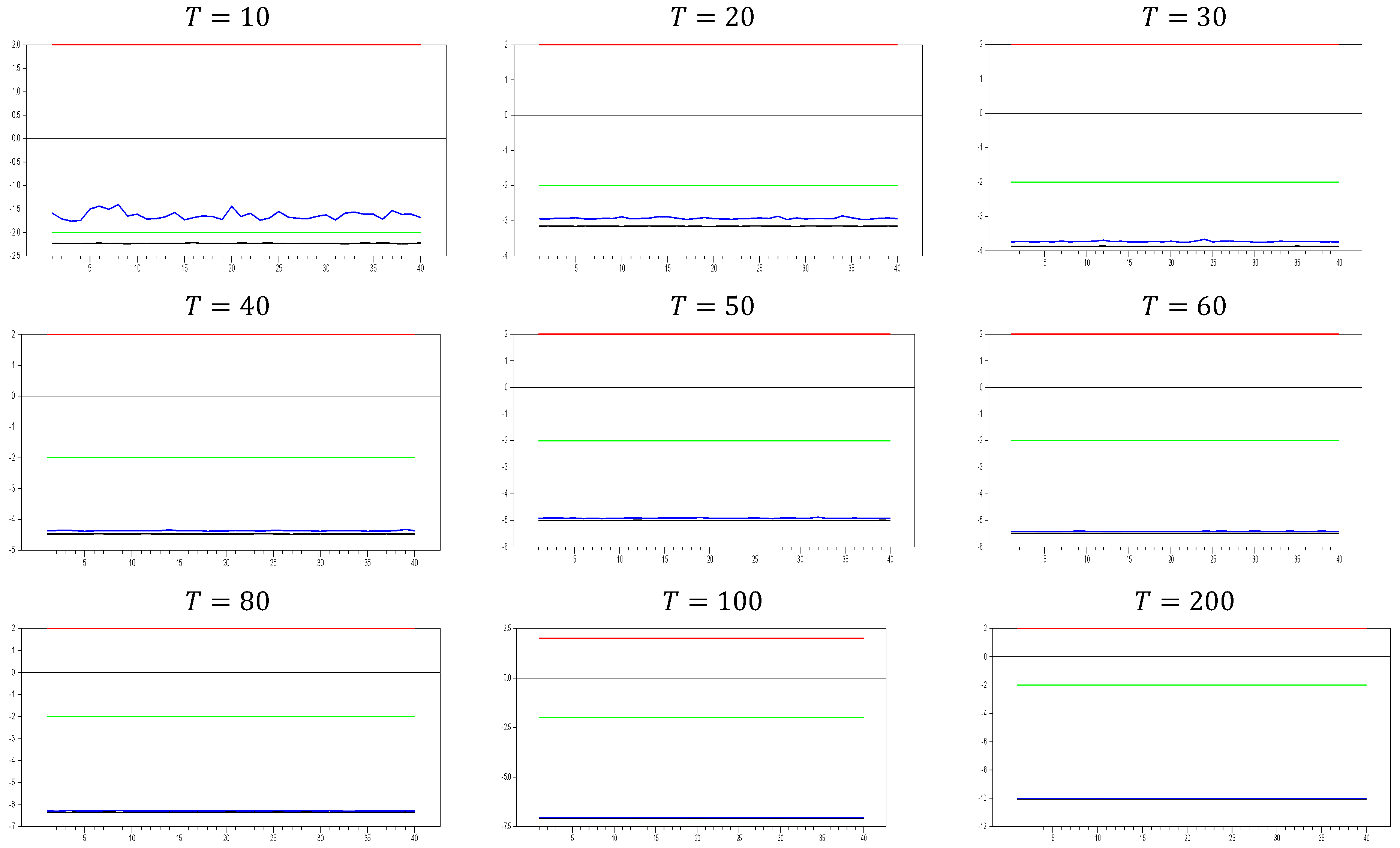
The newly proposed estimator behaves similarly to the CCE estimator for $N=10$. All characteristics, such as the decrease in $C{D}_{LM}$ test values as the $T$ dimension increases and the narrowing of the band, follow the same pattern. However, while the lower bound of the $C{D}_{LM}$ test aligns in both methods, the upper bound converges more slowly than in the CCE estimator. This slower convergence of the upper bound makes the new estimator perform better than the CCE estimator in terms of the $C{D}_{LM}$ test.

In the second step, we increase the $N$ dimension again to assess its impact. The results of these simulations are shown in Figure 22 below. The new proxy method exhibits very similar behavior to the original factor variable for $N=50$, further supporting its effectiveness as a good proxy. In particular, for small $T$ dimensions ($T=10$ to $T=60$), the method performs as well as the original factor. However, for low levels of CSD, such as ${\lambda }_i=\left[\mathrm{0.0,0.01}\right]$, this method does not remedy CSD, which can be seen as a favorable characteristic. Similarly to the CCE estimator, the $C{D}_{LM}$ test shows a negative sign, indicating that the method introduces some CSD. Additionally, as $T$ increases, the upper and lower bounds of the computed values converge to those of the CCE estimator. As $N$ grows, the $C{D}_{LM}$ test results follow the same trend as the CCE estimator. For instance, with $N=100$ and $T=10$0, the lower bound of the $C{D}_{LM}$ test reaches 10.0, while the upper bound also becomes closer to the CCE estimator. This convergence is a positive attribute for deriving the asymptotic properties of the new estimator, showing that as $N$ and $T$ approach infinity, the new test aligns with the same asymptotic properties. The following simulation results are obtained for $N=100$.

From Figure 23, we can clearly observe that for $N=100$ and $T=\left\{\mathrm{80,100}\right\}$, the newly proposed method closely approximates the original factor variable. These simulation results indicate that our proposed method performs similarly to the original factor as $N$ increases while $T$ is fixed. Additionally, we conducted simulations for two scenarios: one where both $N$ and $T$ approach infinity, and another where $T$ is fixed and $N$ is large.

Figure 24 shows that as $N$ and $T$ approach infinity, the new method converges toward the CCE method in remedying CSD.

Figure 24. $C{D}_{LM}$ test results with remedying the CSD by the new method for $N=200$ and $T=1000$.

However, when $T$ is fixed and $N$ approaches infinity, the newly proposed method serves as a better proxy for the original variable. The results for this case are presented in Figure 25.

Figure 25. $C{D}_{LM}$ test results with remedying the CSD by the new method for $N=150$ and $T=100$.

2.4. The Critical Values of the New Refined CCE Estimator and the Finite Sample Properties

Thus, the newly proposed estimator proves to be efficient, falling between the CCE estimator and the original factor in terms of performance. We calculated the critical values for the intercept-only case, which are presented in Table 1.

Table 1. Exact critical values of ${\overline{t}}_{1p,\alpha }$ statistics.

T/N	5	10	15	25	50	70	100
%1
10	−2.280	−2.048	−2.019	−1.898	−1.855	−1.818	−1.798
20	−2.384	−2.268	−2.181	−2.126	−2.072	−2.048	−2.030
30	−2.522	−2.364	−2.257	−2.208	−2.109	−2.111	−2.094
50	−2.622	−2.419	−2.327	−2.260	−2.131	−2.150	−2.199
70	−2.696	−2.440	−2.349	−2.275	−2.179	−2.153	−2.188
100	−2.715	−2.494	−2.393	−2.283	−2.209	−2.181	−2.191
%5
10	−1.916	−1.825	−1.760	−1.704	−1.686	−1.665	−1.665
20	−2.130	−2.038	−2.000	−1.961	−1.938	−1.924	−1.916
30	−2.231	−2.142	−2.087	−2.037	−1.982	−2.000	−1.995
50	−2.347	−2.215	−2.162	−2.106	−2.004	−2.051	−2.007
70	−2.395	−2.224	−2.177	−2.123	−2.062	−2.059	−2.100
100	−2.428	−2.273	−2.201	−2.153	−2.083	−2.068	−2.097
%10
10	−1.735	−1.679	−1.640	−1.603	−1.587	−1.575	−1.574
20	−1.987	−1.937	−1.910	−1.873	−1.858	−1.850	−1.845
30	−2.077	−2.024	−1.976	−1.959	−1.905	−1.928	−1.929
50	−2.206	−2.092	−2.058	−2.018	−1.930	−1.978	−2.040
70	−2.255	−2.119	−2.085	−2.046	−1.997	−1.995	−2.039
100	−2.282	−2.155	−2.107	−2.077	−2.011	−2.019	−2.036

The distribution appears to be slightly flawed, but it converges to the distribution from [8] when $N=100$ and $T=100$. The critical values for the 1%, 5%, and 10% significance levels in [8] are −2.15, −2.07, and −2.02, respectively, while for our proposed method, they are −2.19, −2.09, and −2.03. This pattern is illustrated in Figure 21, Figure 22, Figure 23 and Figure 24. Based on these critical values, we compare the finite sample performances of the two estimators.

First, following the DGP outlined in [8], we conduct an empirical size analysis comparing our newly proposed estimator with the estimator from [8]. The results are given in Table 2. We use 2000 replications to compute the empirical size of the tests at the 5% nominal level. Table 2 shows that both of the methodologies exhibit good size properties. Fortunately, our methodology has slightly better size properties, especially for small $T$ values.

Table 2. Size comparison under the strong cross-sectional dependency.

$\mathit{T}/\mathit{N}$	10		25		50		100
	CCE	RCCE	CCE	RCCE	CCE	RCCE	CCE	RCCE
10	0.057	0.050	0.059	0.051	0.060	0.053	0.061	0.055
30	0.061	0.049	0.058	0.050	0.059	0.055	0.057	0.056
50	0.054	0.050	0.059	0.052	0.058	0.053	0.062	0.055
70	0.054	0.054	0.059	0.051	0.059	0.054	0.058	0.055
100	0.056	0.052	0.057	0.053	0.060	0.054	0.059	0.056

Note: RCCE denotes refined CCE estimator.

Next, Table 3 presents the empirical power of both methodologies under the strong cross-sectional dependency. The results from Table 3 clearly indicate that when $N\to \mathrm{\infty }$ and $T\to \mathrm{\infty }$, increasing the empirical power of our proposed test is better than the CCE estimator. In short, for only small $N$ and $T$, the empirical power of the CCE estimator is better than our test.

Table 3. Power comparison under the strong cross-sectional dependency.

T/N	10		25		50		100
	CCE	RCCE	CCE	RCCE	CCE	RCCE	CCE	RCCE
10	0.069	0.059	0.087	0.117	0.169	0.146	0.270	0.207
30	0.209	0.097	0.302	0.302	0.488	0.489	0.666	0.539
50	0.428	0.193	0.632	0.632	0.886	0.917	0.965	0.969
70	0.719	0.432	0.959	0.959	0.998	1.000	1.000	1.000
100	0.954	0.816	1.000	1.000	1.000	1.000	1.000	1.000

3. Empirical Study

In this empirical section, we apply our methodology to identify new proxy variables for the original factor used in the methodology. For the empirical analysis, we used unemployment rate data for four Nordic countries, sourced from the FRED (Federal Reserve Economic Data) database, covering the period from 2001Q1 to 2015Q2.

In the unemployment rate, we can clearly see that the CADF test incorrectly rejects the true null hypothesis from Table 4.

Table 4. Four Nordic Countries’ Unemployment Rate.

	RCCE	CADF
Test Results	−1.874	−2.493 ***
%1	−2.715	−3.022
%5	−2.422	−2.645
%10	−2.270	−2.467

Note: *, **, *** denote the rejection of null hypothesis at 10%, 5%, and 1%, respectively.

Figure 26 shows that the unemployment data include a structural break, yet the CADF test still rejects the null hypothesis. It is well known that when structural breaks are present, methods that do not account for de-trending are less powerful. This suggests a size problem, as noted in the small-sample performance. The slightly better performance of the RCCE test demonstrates its superiority in this empirical analysis. As shown in [31], the CCE estimator of [8] produces incorrect results in homogeneous structural break-type DGPs, and this empirical study supports the findings of [31].

Figure 26. Nonlinear trends for four Nordic countries.

4. Concluding Remarks

In this study, we examine the features of the CCE estimator in panel data models, particularly in the context of nonstationary panels. While cross-sectional dependence and its remedies have been analyzed in various studies through bias estimation, our approach utilizes the cross-sectional dependence test. This simple approach offers an advantage over other studies, as we also assess the reliability of the $C{D}_{LM}$ test. Based on our simulation results, we propose new proxy variables for CCE estimation. These new variables and estimators can be considered refinements of the CCE estimator in panel unit root models.

As stated in [29], including additional variables in panel unit root testing to remedy CSD can increase the correlation between regressors and proxy factor variables, which is a major drawback of the CCE estimator. Based on this, we proposed a simpler estimator that uses only the average of the dependent variable without taking the first difference. The simulation study showed promising results for very small $N$ values, but for larger $N$, the newly proposed method performed worse than the CCE estimator. In response to [29]’s criticism, we developed a two-stage estimator. In the first stage, we use the CCE estimator to avoid increasing the correlation between the regressors and factor variables. In the second stage, we incorporate an auxiliary regressor generated from the first stage, following the suggestion of [29]. This newly proposed two-stage method works effectively for both small and large $N$ and $T$ values. The shortcomings of the CCE estimator, as mentioned by [29], are further examined in the empirical section. We compared the unit root test results of the new estimator with those of [8]’s test, focusing on data with structural breaks. While [8]’s test indicated that the series under investigation was stationary, it failed to account for the structural breaks in the DGP. In contrast, our newly proposed test accurately identified the presence of a unit root problem. As a result, our methodology eliminated size bias.

All of these simulation studies and empirical results demonstrate that there is still room for developing new estimators to address the cross-sectional dependence problem in panel unit root tests. For future research, scholars can explore nonlinear functional forms or similar methodologies to see if they can further mitigate the CSD issue in panel unit root testing. Fortunately, our new $C{D}_{LM}$ test simulation approach provides a simple framework that will facilitate the design of more complex simulation studies.