Abstract
The purpose of this paper is to investigate some Morse-type oscillators. In its original form, it is a model for describing the vibrations of a diatomic molecule. The Morse potential generalizes the harmonic oscillator by introducing deviations from the classical theoretical model. In the present study, we perturbed the Morse differential equation by several periodic terms based on the function and by a damping term. The frequency is driven by different coefficients. The size of the deviations is controlled by another constant. We provide two modifications w.r.t. the damping term. The Melnikov approach is applied as an indicator of the possible chaotic opportunities. We also propose a novel approach for stochastic control of the perturbations. It is based on the assumption that the coefficients of the periodic terms are the probabilities of underlying distribution. As a result, the dynamics are driven by its characteristic function. Several applications are considered. We demonstrate some specialized modules for investigating the dynamics of the proposed models, along with the synthesis of radiating antenna patterns.
MSC:
34C37
1. Introduction
A number of authors have devoted their research to the classical Morse [1] oscillator. The reader can find detailed information about the dynamics of the Morse oscillator—analytical expressions for trajectories, action–angle variables, and chaos dynamics—in the magnificent studies [1,2,3,4,5,6]. The driven Morse oscillator is an equation frequently used in theoretical chemistry to describe the photodissociate of molecules [5]. The equation is given by
with initial conditions , , where and . From the Hamiltonian, taking as a fixed value h, we can see that . The homoclinic orbit is the solution for which (see Figure 1). For , is a nonhyperbolic fixed point of (1) that is connected to itself by a homoclinic orbit. We would like to apply Melnikov’s theory [7] to (1) in order to see if (1) has horseshoes; however, the fixed point having the homoclinic orbit is nonhyperbolic. Therefore, the classical theory does not immediately apply. Schecter [8] has extended Melnikov’s method so that it applies to nonhyperbolic fixed points. The following transformation of variables is known:
(see, for example, Ref. [3] (p. 722)), where the resulting equation with new variables is
where .
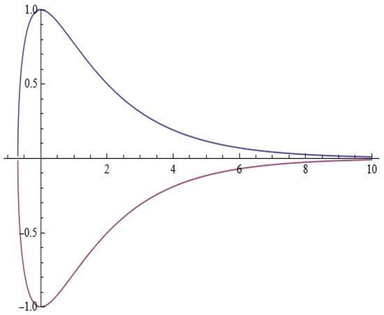
Figure 1.
The homoclinic orbit.
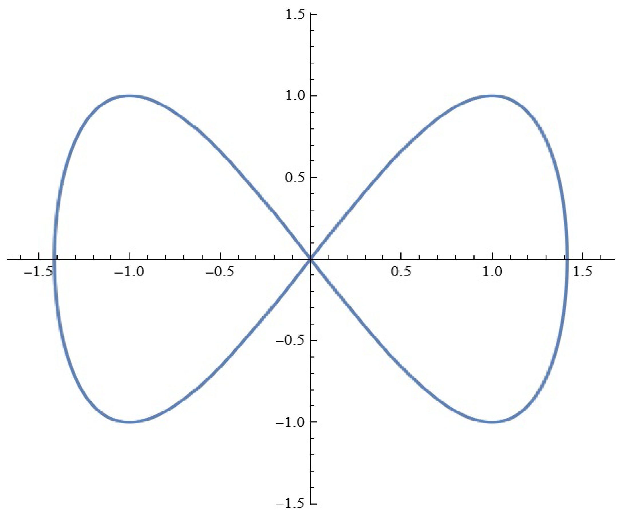
For , Equation (3) has a hyperbolic fixed point at the origin that is connected to itself by a homoclinic orbit (see Figure 2).
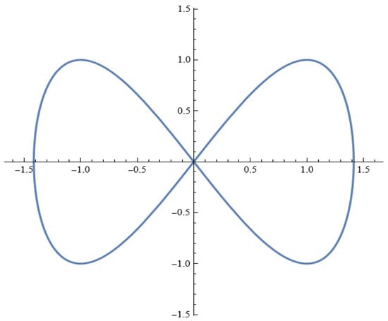
Figure 2.
The homoclinic orbit.
This problem was originally solved by Bruhn [6]. The transformation (2) is known as a “McGehee transformation” [9]. In [10], the author investigated the following model:
In our article, we have used Melnikov’s approach [7] on a novel modified Morse type oscillator to identify the existence of chaotic behavior into it. We developed specific modules for the dynamics research of these hypothetical oscillators. The obtained outcomes can be useful as an integral part of application for numerical computations—for more specifics, see [11,12,13,14]. Some interesting results can be found in [15,16,17].
To introduce a specific structure for the perturbations, we assume that their components are governed by a discrete stochastic distribution via its probabilities. As a particular examples, we investigated several examples based on binomial, -binomial, and geometric distributions.
The plan of the paper is as follows. We state our models in Section 2 and investigate them in light of Melnikov’s approach. In addition, we discuss the considered models driving the perturbations through a stochastic distribution. Some possible applications are provided in Section 3. We conclude in Section 4. For specialists working in the field of antenna array theory, we provide in Appendix A an explicit presentation of the Melnikov function for what we tentatively call Model B in this particular case.
2. Some New Models — Some Simulations
2.1. Model A
We consider the following new modified model of the form:
with initial conditions , , where , and is integer.
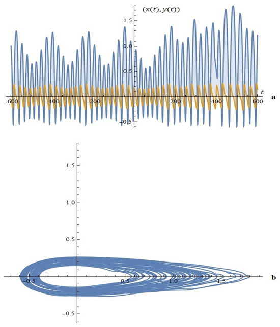
Example 1.

Figure 3.
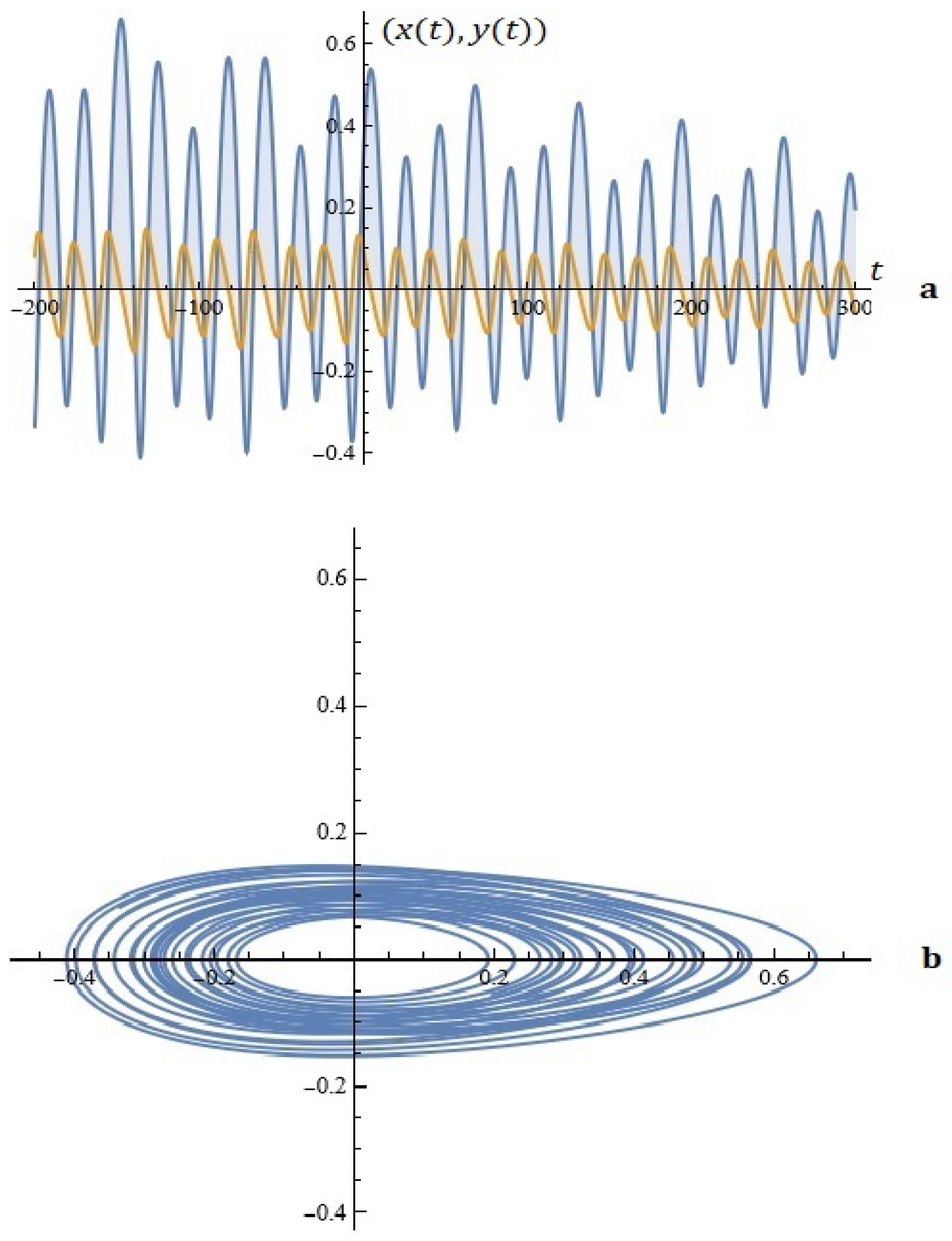
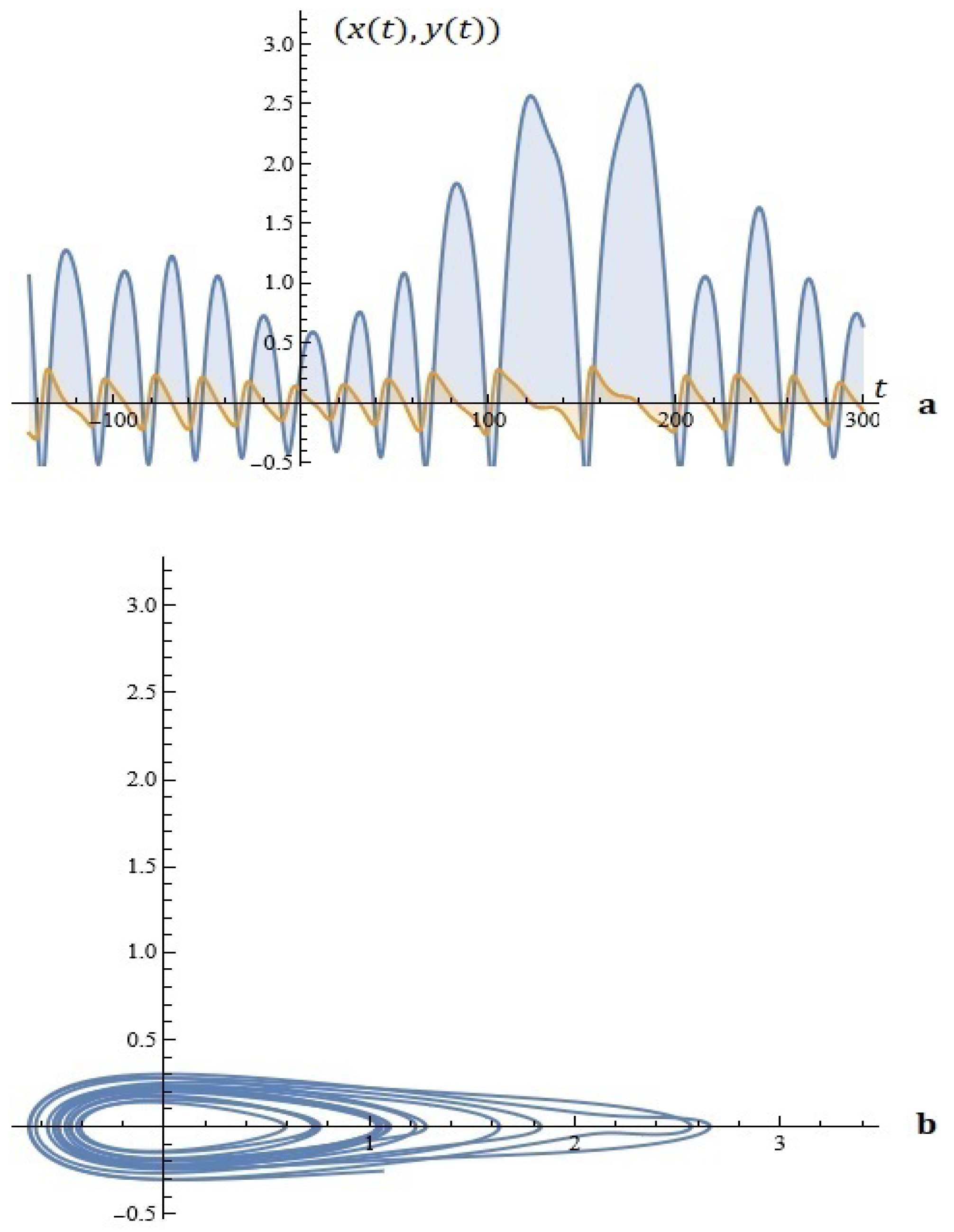
(a) The solutions of system (5). (b) Phase space (Example 1).
Example 2.

Figure 4.
(a) The solutions of system (5). (b) Phase space (Example 2).
Example 3.
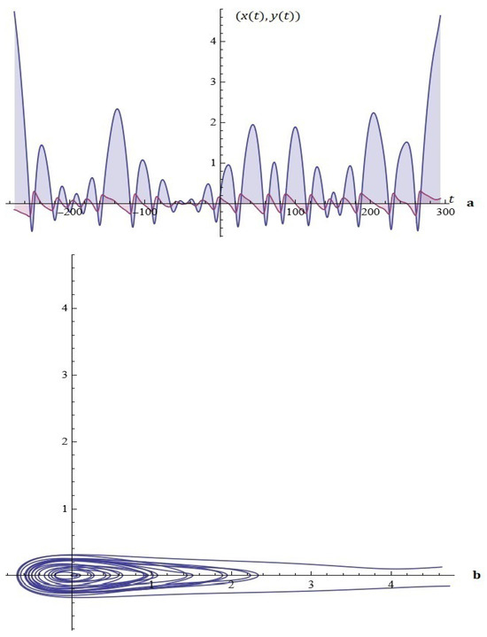
Figure 5.
(a) The solutions of system (5). (b) Phase space (Example 3).
2.1.1. Considerations in Light of Melnikov’s Approach
The Melnikov function provides a measure of the leading order distance between the stable and unstable manifolds when and can be used to tell where the stable and unstable manifolds intersect transversely.
We can prove the following proposition.
Proposition 1.
The roots of Melnikov function are given as solutions of the nonlinear equation
Proof.
We see that . Here, is the integration constant that corresponds to the initial time. The integral of Melnikov is given by
where the functions and are defined in Equation (4). After the substitution
we find
where .
Evidently,
From
we have
□
This completes the proof of Proposition 1.
Note. We will explicitly note that in the proof of Proposition 1 we have used methodological studies detailed in works [1,10].
From a numerical point of view, the task of finding the roots of are more interesting given that the parameters appearing in the proposed differential model are subject to a number of restrictions from the field of theoretical chemistry.
If and for some and some sets of parameters, then chaos occurs.
Clearly, in the case , the Melnikov function has ”simple zeros”, indicating the existence of homoclinic orbit and the associated Smale horseshoe type chaos. For details, see [1].
For example, fixing , the equation is depicted in Figure 6.
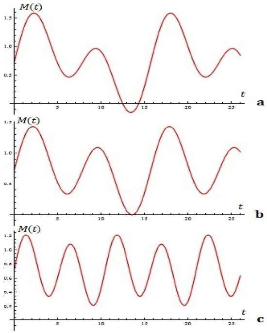
Figure 6.
The equation (the case ).
For , the roots are and (see Figure 6a).
For , the root with multiplicity two is (Figure 6b).
For , there are no roots (see Figure 6c).
Fixing , , the equation is depicted in Figure 7.

Figure 7.
The equation (the case ).
Fixing , , , the equation is depicted in Figure 8.
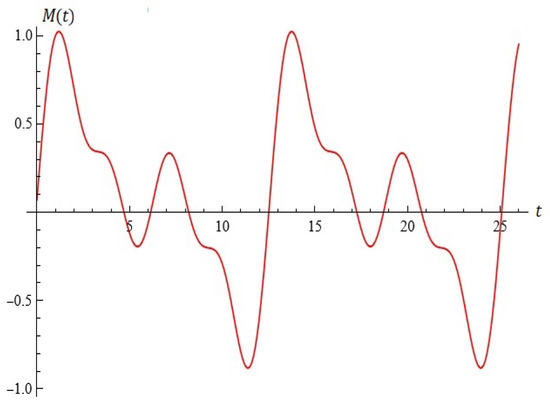
Figure 8.
The equation (the case ).
From Proposition 1, for any fixed N, the reader may formulate the Melnikov criterion for the appearance of the intersection between the perturbed and unperturbed separatrixes.
2.1.2. Probability Distributions Driving the Perturbation
Suppose now that the coefficients that drive the perturbation in oscillator (5) are the probabilities of some discrete distribution supported on the set . We can assume this without loss of generality after scaling for . Let be a random variable distributed under this law and be its characteristic function. Some most popular choices are the discrete uniform, binomial, -binomial, and hypergeometric distributions. For some similar constructions, we refer to [14]. In addition, if we obtain an infinite but countable set of ’s imposing the condition , then we can use a discrete distribution stated on the infinite support —for example, the geometric distribution.
Having in mind the well-known complex presentation of the cos-function
we rewrite oscillator dynamics (5) as
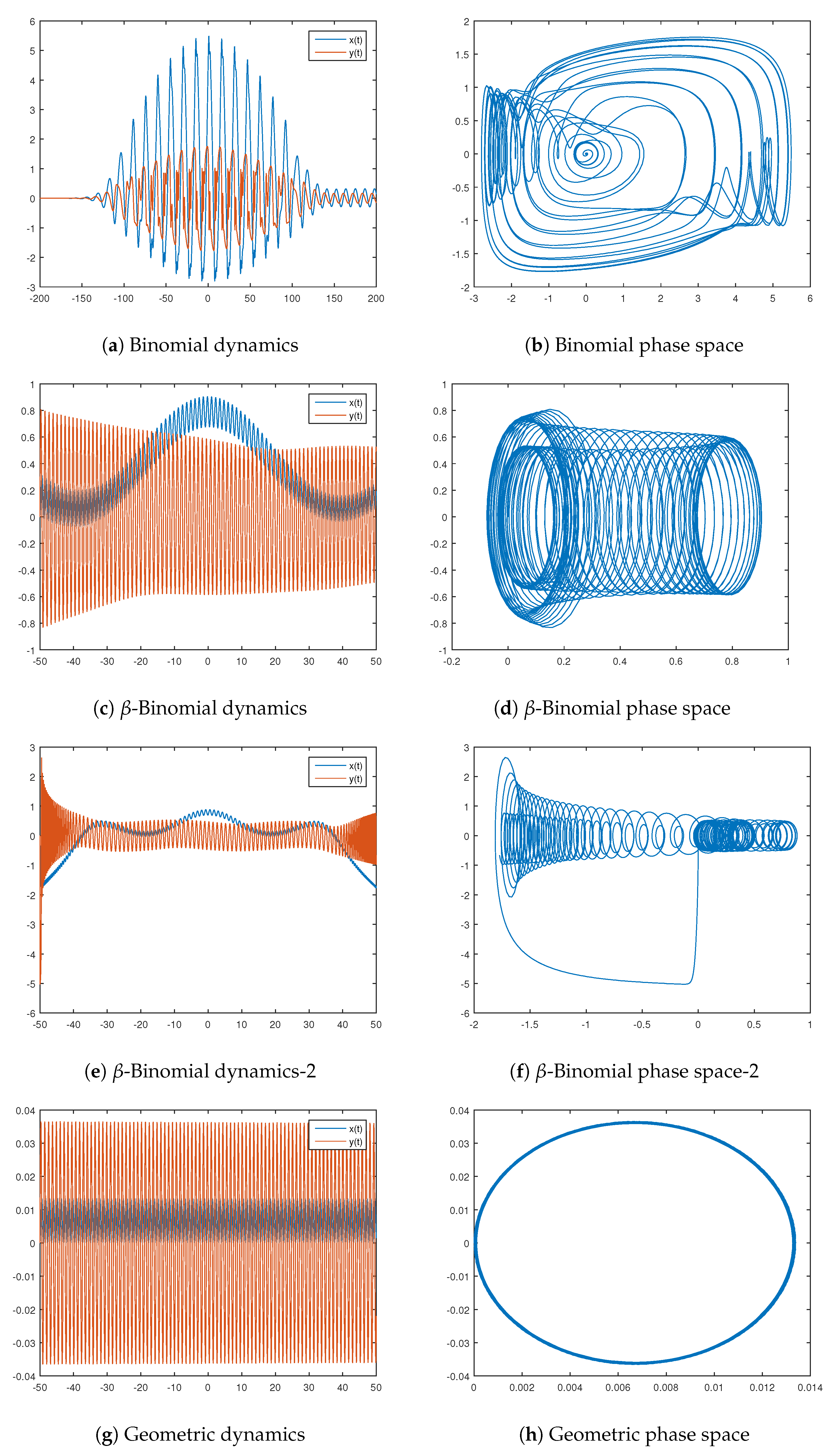
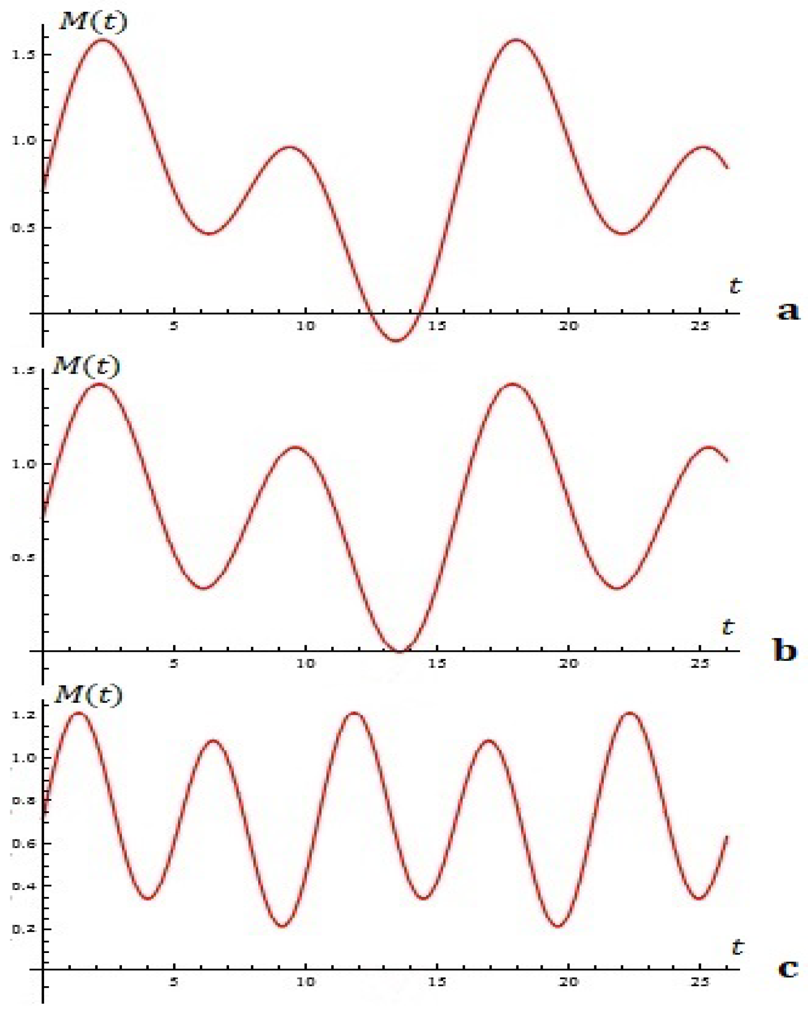
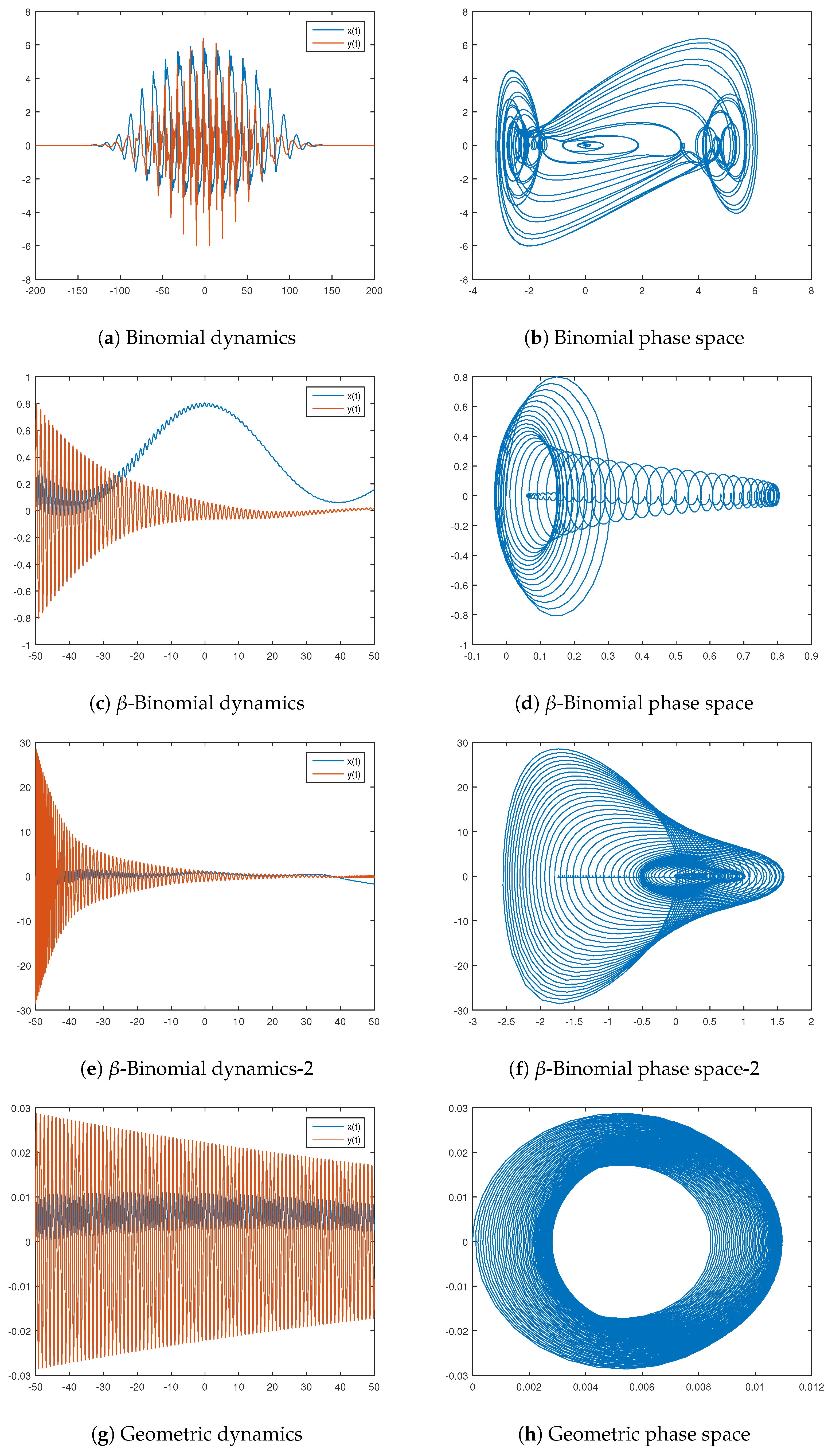
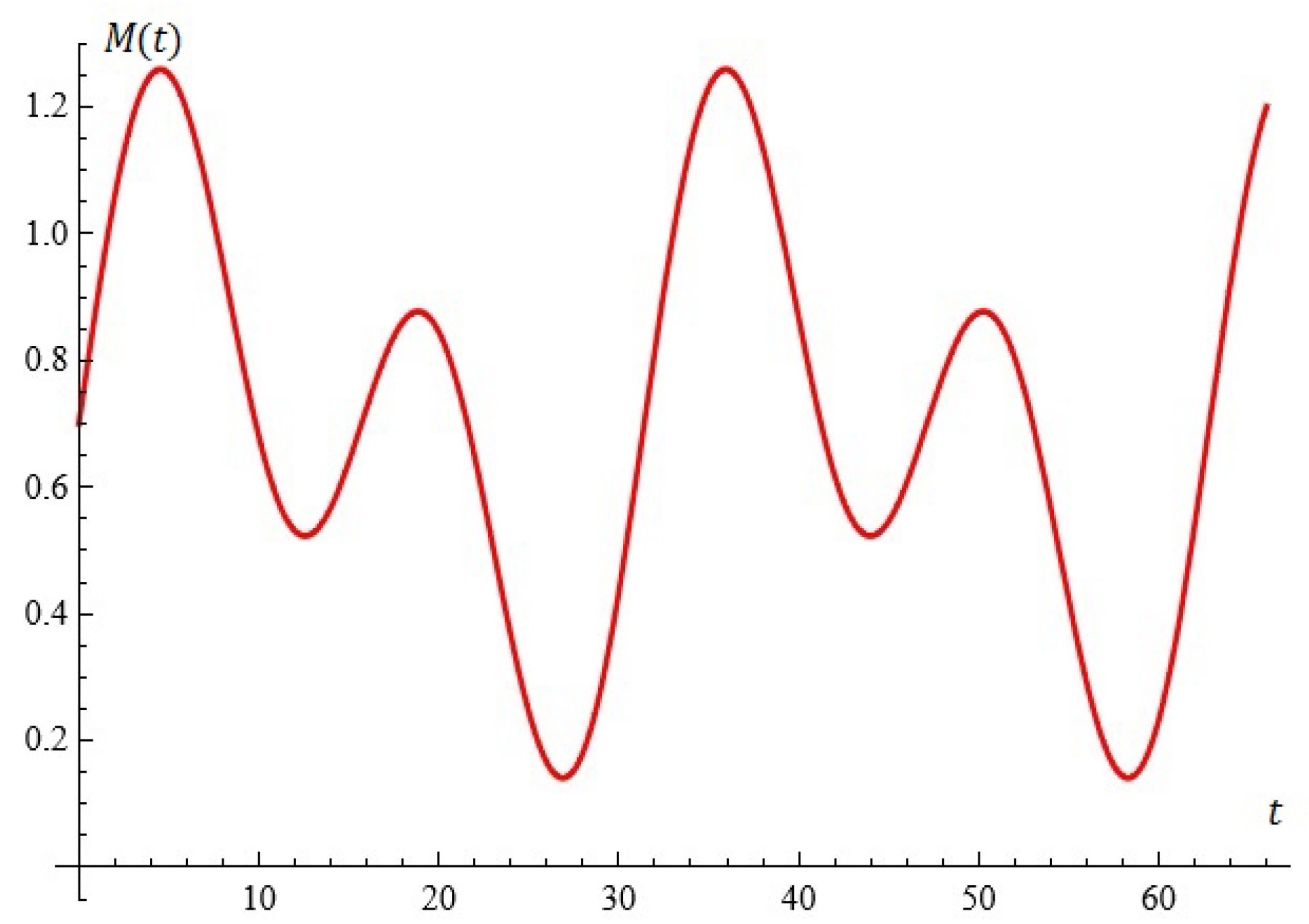
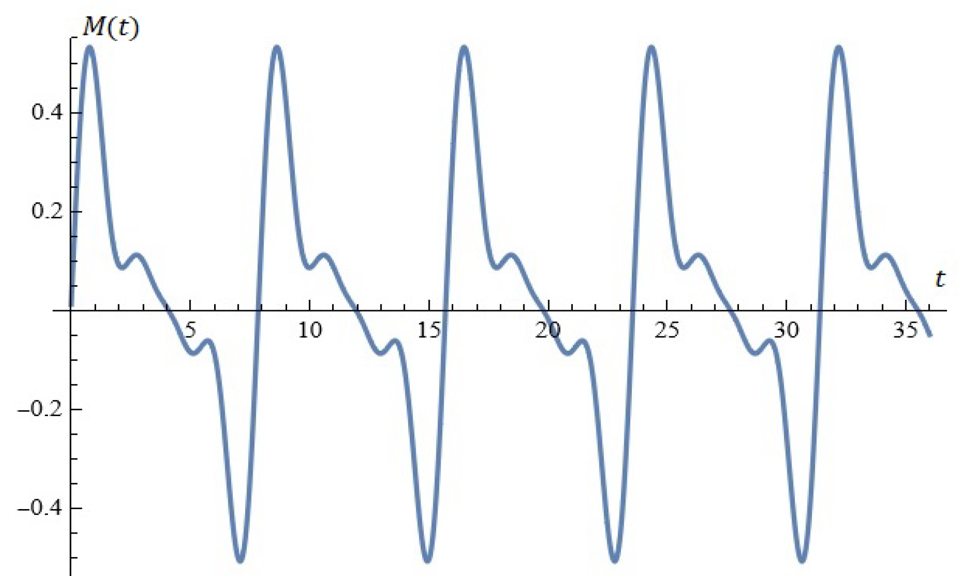
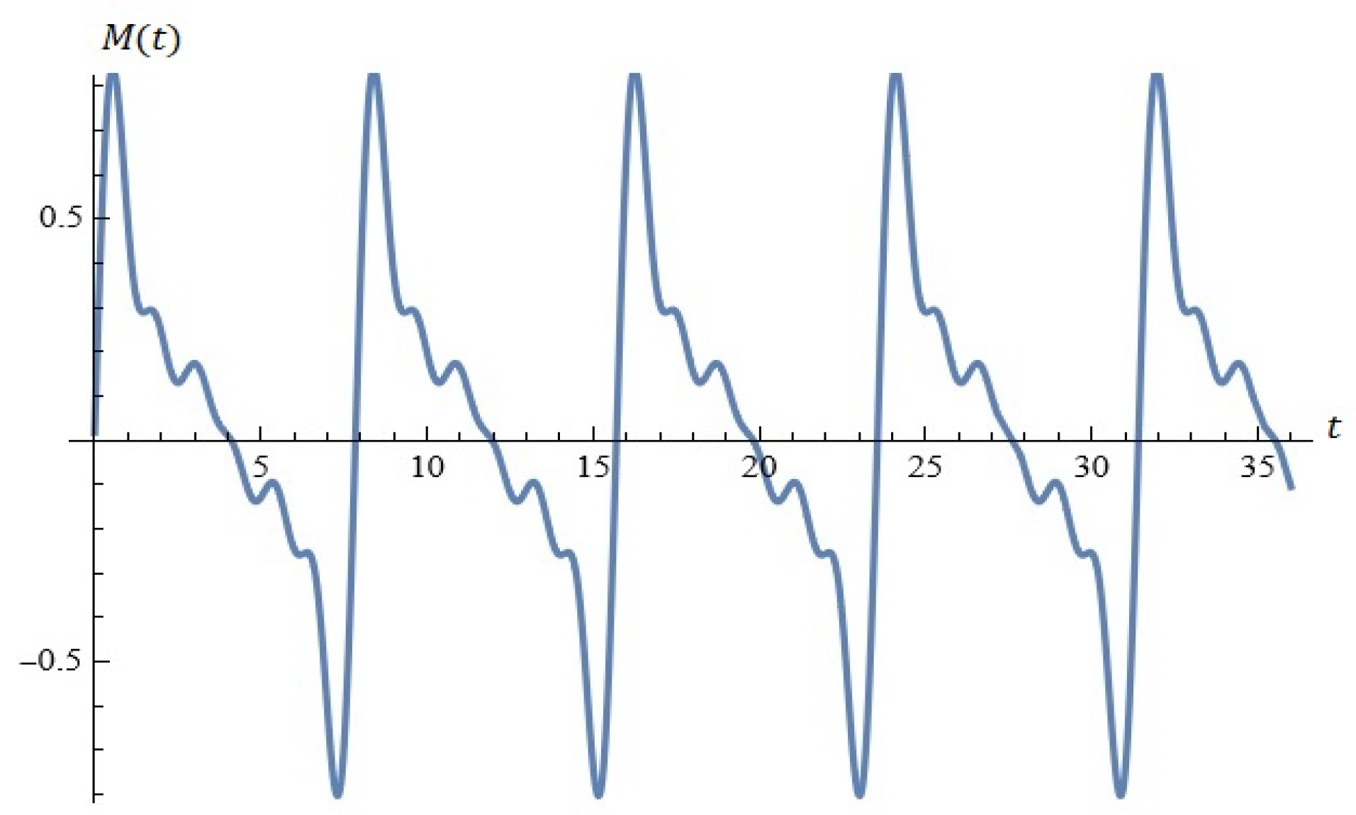
Let the scaling coefficient be denoted by . We present four examples in Figure 9 based in binomial, -binomial, and geometric distributions. Their characteristic functions are
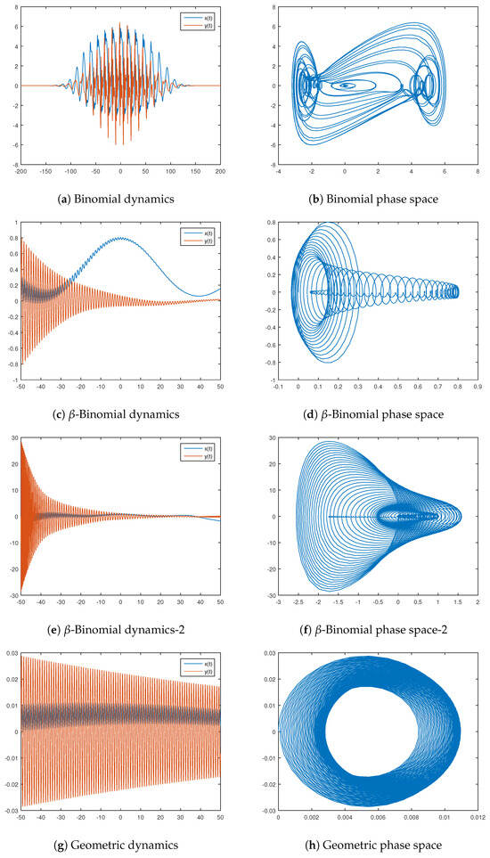
Figure 9.
Oscillators based on the binomial and -binomial distributions.
The used parameters for the provided examples are as follows:
- Binomial distribution: , , , , , , ;
- -Binomial distribution: , , , , , , ;
- -Binomial distribution: , , , , , , ;
- Geometric distribution: , , , , , .
Note that the -binomial examples differ only by the number of trials—we consider or . We can see in Figure 9c–f the similarities and differences in the dynamics they generate.
Let us consider Proposition 1. Using the complex form of the sin-function,
we see that the Melnikov function (6) can be rewritten as
Thus, Equation (6) can be rewritten as
2.2. The Model B
We consider the following new modified model of the form:
with initial conditions , , where , , is integer, and is the damping exponent.
We will look at some interesting simulations of model (9):
Example 4.
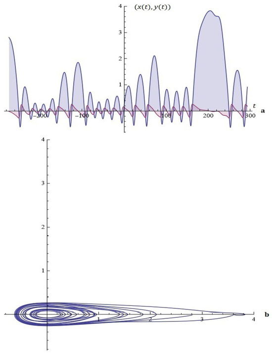
Figure 10.
(a) The solutions of system (9). (b) Phase space (Example 4).
Example 5.
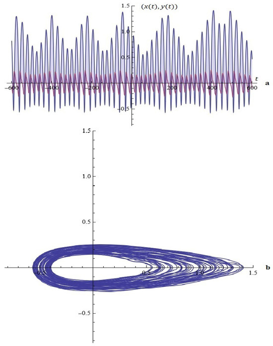
Figure 11.
(a) The solutions of system (9). (b) Phase space (Example 5).
Considerations in Light of Melnikov’s Approach
We can prove the following propositions:
Proposition 2.
For fixed , the roots of Melnikov function are given as solutions of the nonlinear equation
Examples. For fixed , :
- (i)
- For , the equation is depicted in Figure 13.
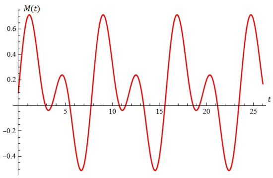 Figure 13. The equation (Proposition 2; case (i)).
 - (ii)
- For , the equation has a root with multiplicity two (see Figure 14).
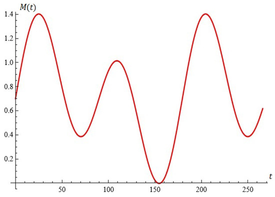 Figure 14. The equation (Proposition 2; case (ii)).
 - (iii)
- For , the equation has no roots (see Figure 15).
 Figure 15. The equation (Proposition 2; case (iii)).
Proposition 3.
For fixed , the roots of Melnikov function are given as solutions of the nonlinear equation
For example, for , , , , the equation is depicted in Figure 16.
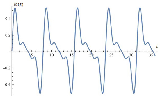
Figure 16.
The equation (Proposition 3).
Proposition 4.
For fixed , the roots of Melnikov function are given as solutions of the nonlinear equation
For example, for , , , , the equation is depicted in Figure 17.
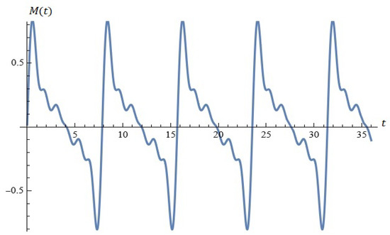
Figure 17.
The equation (Proposition 4).
The proof of Propositions 2–4 follows the ideas given in this article and will be omitted.
3. Possible Applications
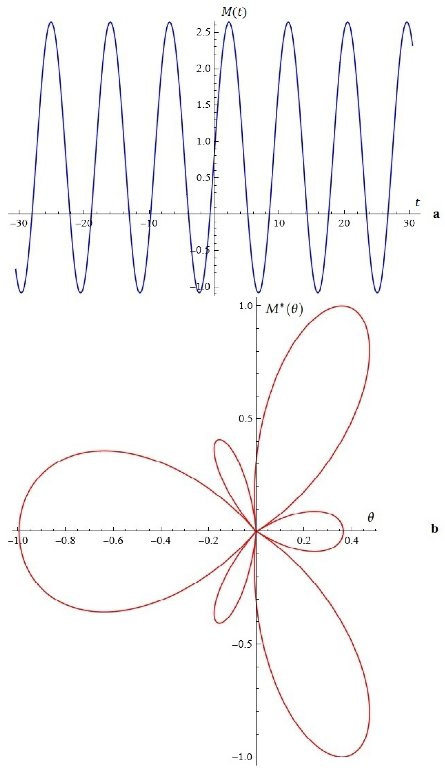
Let us now focus on .
We define the hypothetical normalized antenna factor as follows: + , where is the azimuth angle; is the wave length; d is the distance between emitters; and is the phase difference. For more details and related literature, see [18,19].
Following the classical research by Dolph–Chebyshev, we will call the Melnikov antenna array (see also [13,14]).
Model A.
(case I) For fixed , , (from Proposition 1), see Figure 18.
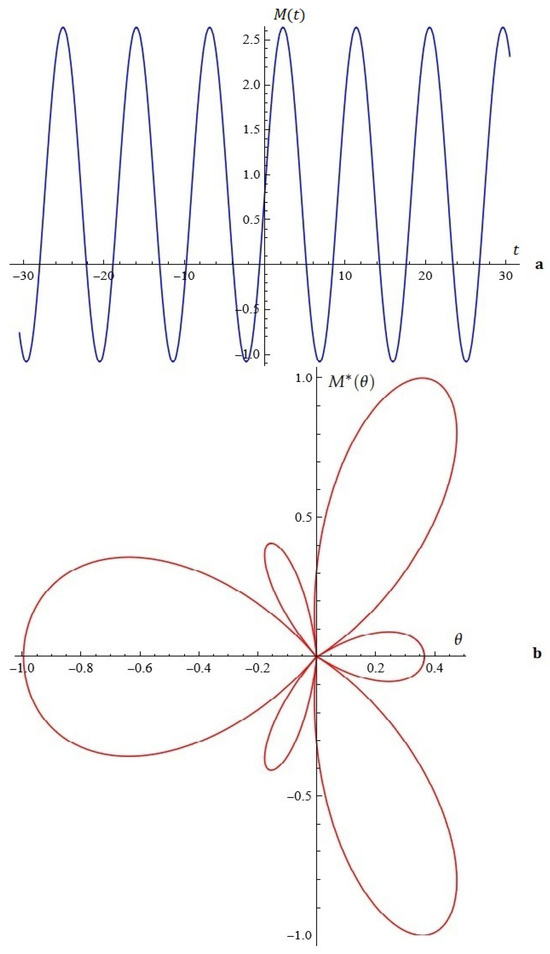
Figure 18.
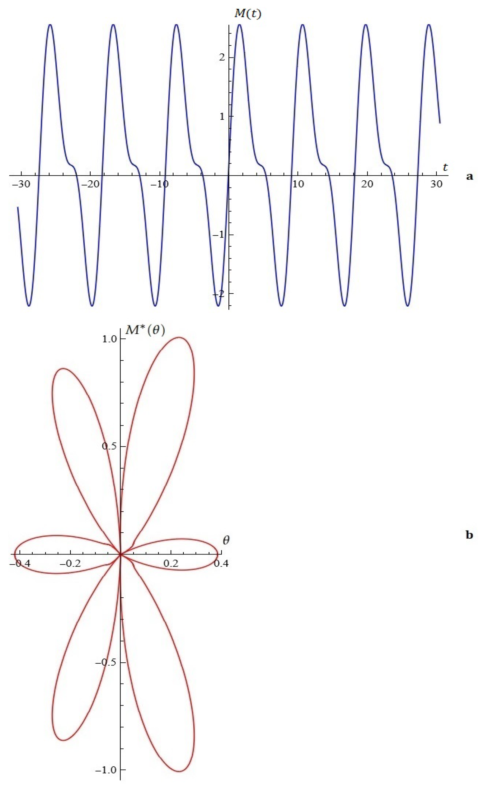
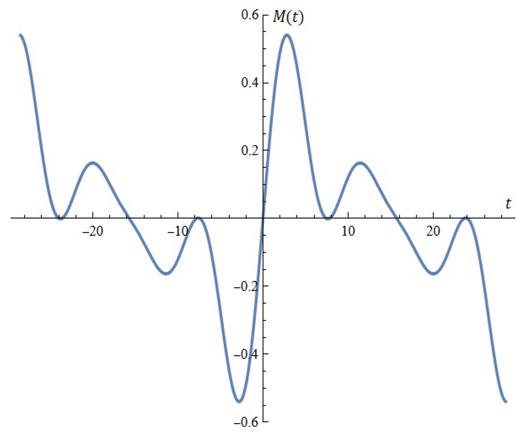
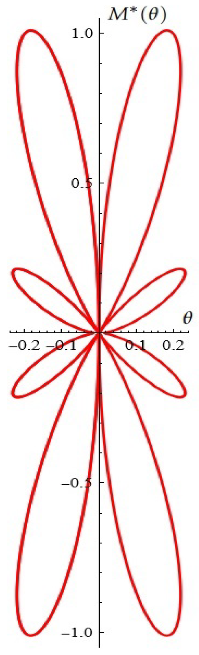
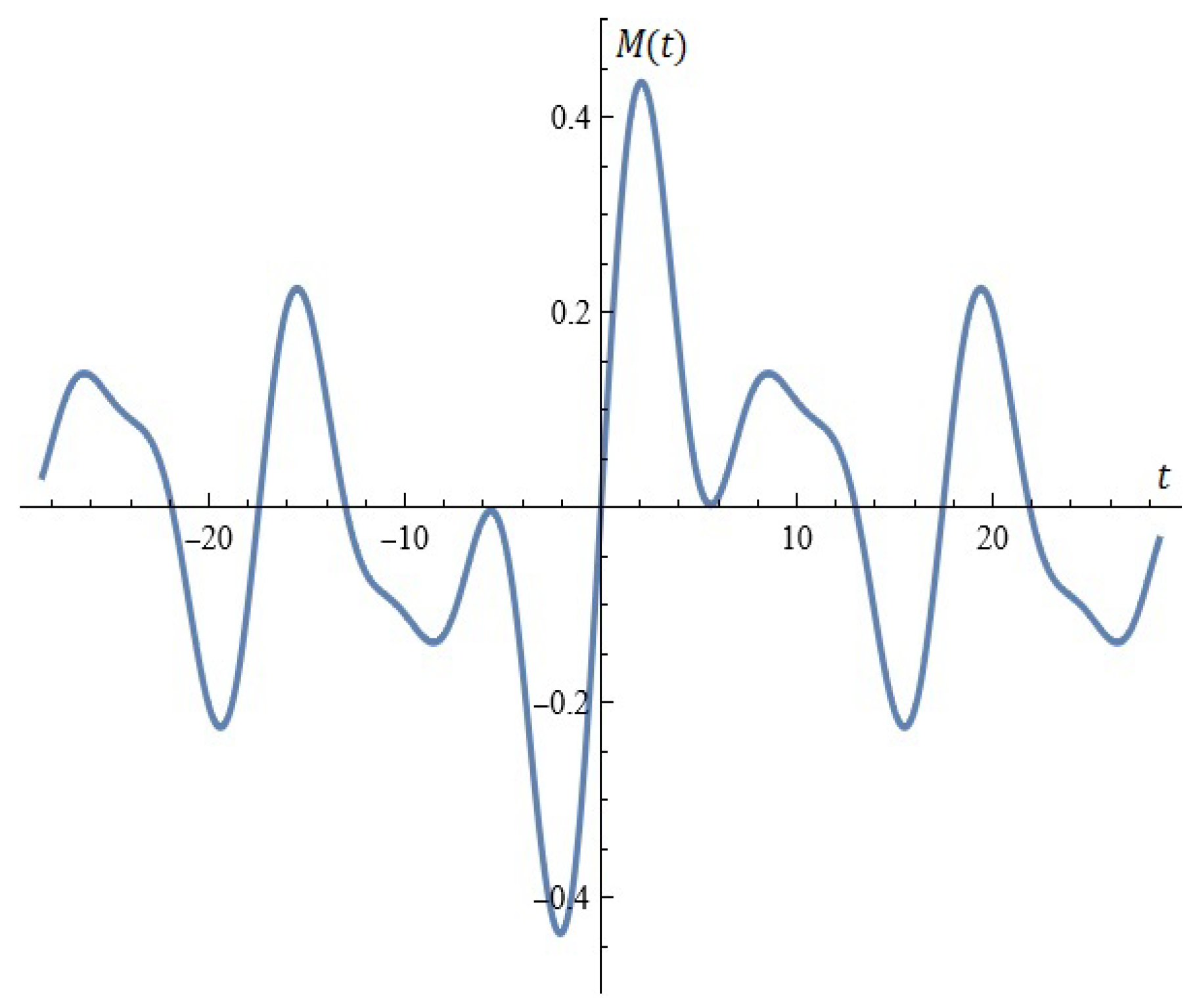
Model A (case I): (a) the Melnikov function; (b) A typical Melnikov antenna array.
(case II) For fixed , , (from Proposition 1), see Figure 19.
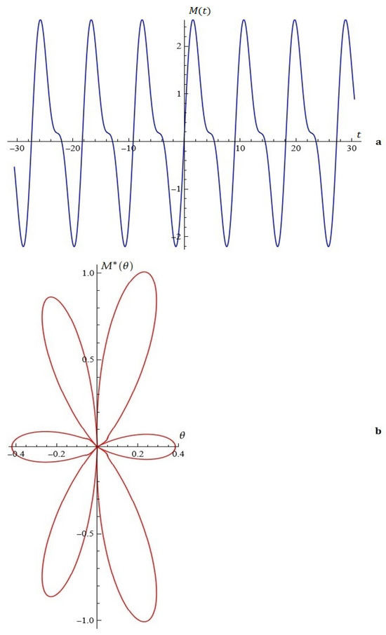
Figure 19.
Model A (case II): (a) the Melnikov function; (b) A typical Melnikov antenna array.
Model B.
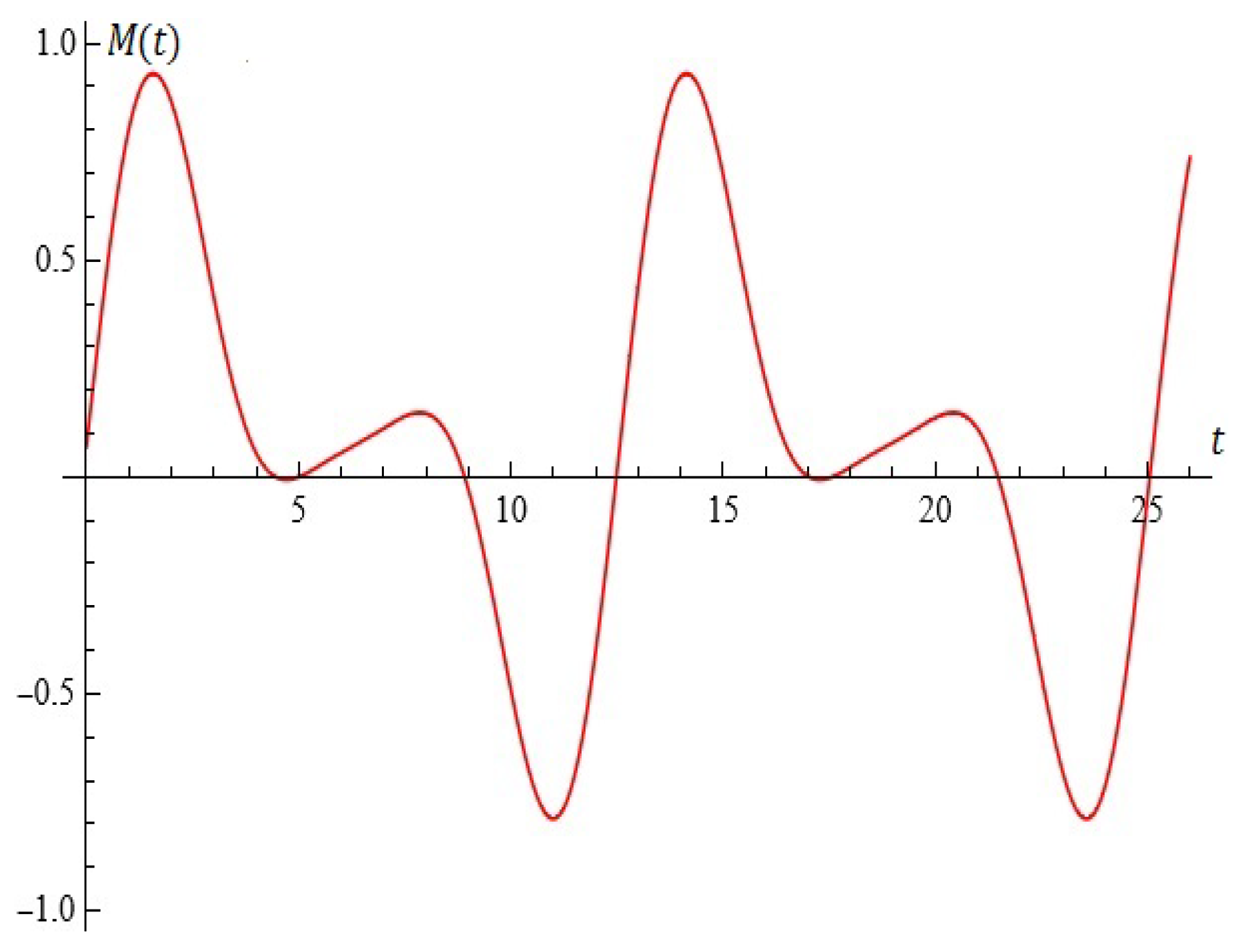
For fixed , , , from Proposition 2, the Melnikov function is depicted in Figure 20. The Melnikov antenna array is depicted in Figure 21.
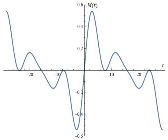
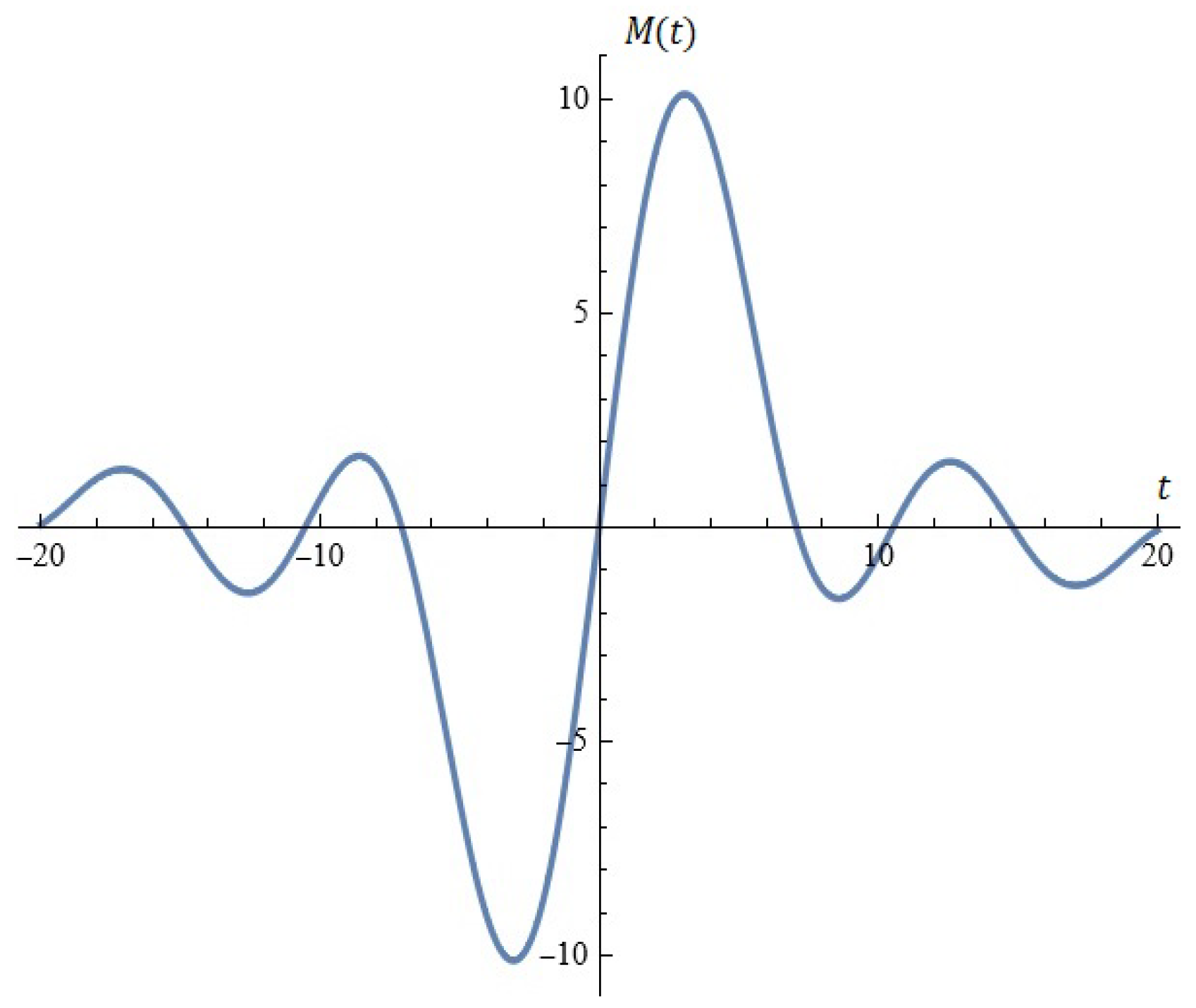
Figure 20.
The Melnikov function.
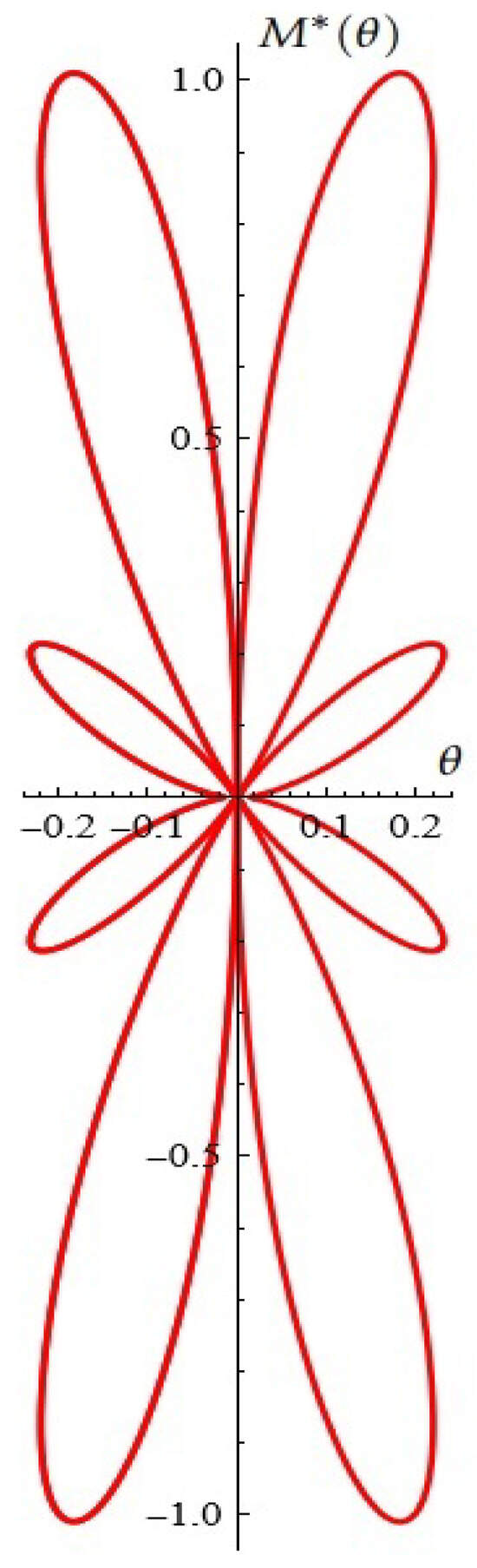
Figure 21.
A typical Melnikov antenna array.
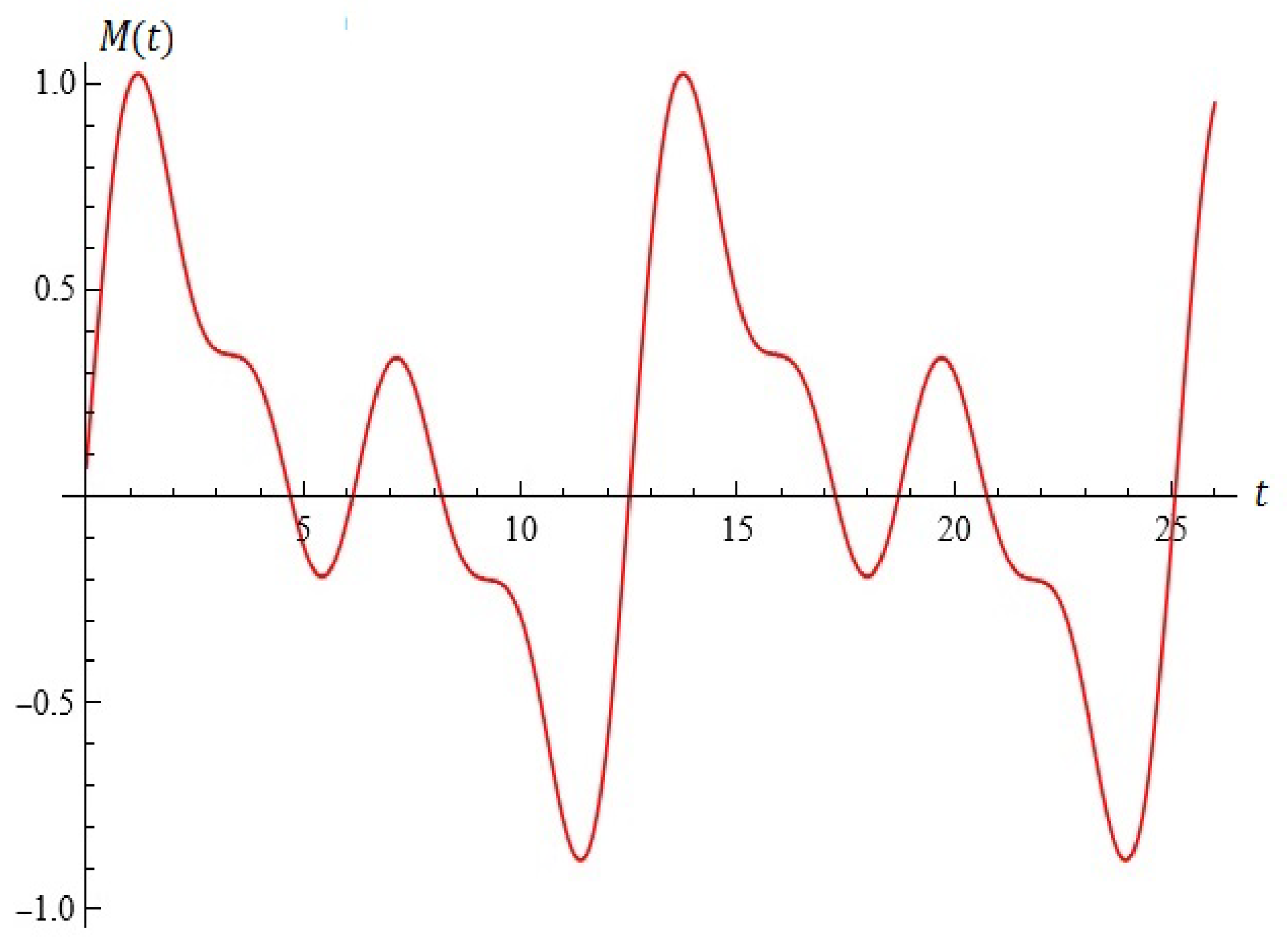
For fixed , , , from Proposition 3, the Melnikov function is depicted in Figure 22. The Melnikov antenna array is depicted in Figure 23.
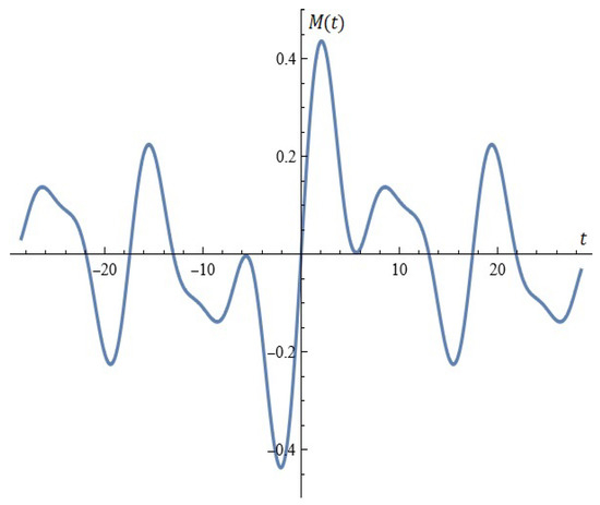
Figure 22.
The Melnikov function.
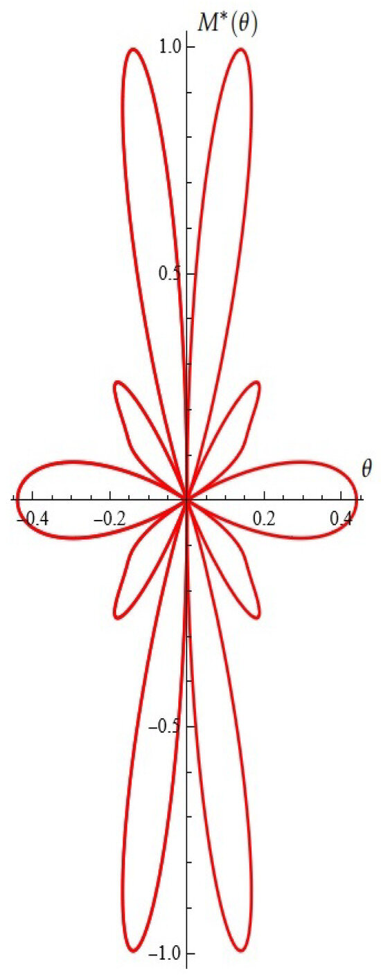
Figure 23.
A typical Melnikov antenna array.
Of course, after serious consideration by specialists working in this scientific direction, the hypothetical Melnikov array proposed by us can be seen as a supplement to the Array Antenna Theory.
4. Conclusions
In this article, we propose a new modified Morse-type oscillator. Investigations in light of Melnikov’s approach is considered. We also demonstrate some specialized modules for investigating the dynamics of these oscillators. This will be included as an integral part of a planned much more general Web-based application for scientific computing.
From a numerical point of view, the task of finding the roots of are more interesting given that the parameters appearing in the proposed differential model are subject to a number of restrictions from the field of theoretical chemistry. Numerical methods for solving nonlinear equations can be found in [20].
Author Contributions
Conceptualization, T.Z. and N.K.; methodology, N.K. and T.Z.; software, T.Z., T.B., V.K. and A.I.; validation, A.R., T.Z., A.I. and T.B.; formal analysis, N.K. and T.Z.; investigation, T.Z., N.K., T.B., A.R. and A.I.; resources, A.R., T.Z., V.K. and N.K.; data curation, T.B., A.R. and V.K.; writing—original draft preparation, V.K., N.K. and T.Z.; writing—review and editing, A.R., T.B. and A.I.; visualization, V.K. and T.B.; supervision, N.K. and T.Z.; project administration, T.Z.; funding acquisition, A.R., T.Z., T.B., N.K. and A.I. All authors have read and agreed to the published version of the manuscript.
Funding
The first, third, and sixth authors are supported by the European Union-NextGenerationEU, through the National Plan for Recovery and Resilience of the Republic of Bulgaria, project No BG-RRP-2.004-0001-C01. The research of the second and fourth authors was carried out under project BG-RRP-2.011-0049, “Integrated Framework for Health Service Improvement via Analysis of Patient Reported Outcomes Data”, funded by the Recovery and Resilience Mechanism as part of investment C2.I2, “Enhancing the Innovation Capacity of the Bulgarian Academy of Sciences in the Field of Green and Digital Technologies”.
Institutional Review Board Statement
Not applicable.
Informed Consent Statement
Not applicable.
Data Availability Statement
Data are contained within the article.
Conflicts of Interest
The authors declare no conflicts of interest.
Appendix A
For specialists working in the field of antenna array theory, the following explicit presentation of the Melnikov function for what we tentatively call Model B will surely be of interest:
where
and
Remarks.
- (i)
- We will explicitly note that the compact record (8) is obtained after applying recursive techniques in the calculation of the Melnikov integral and with the help of a module specially written by us for this purpose and implemented in the CAS Mathematical program environment.
- (ii)
- In some cases, it is convenient to use the following notation for the general term of the series:
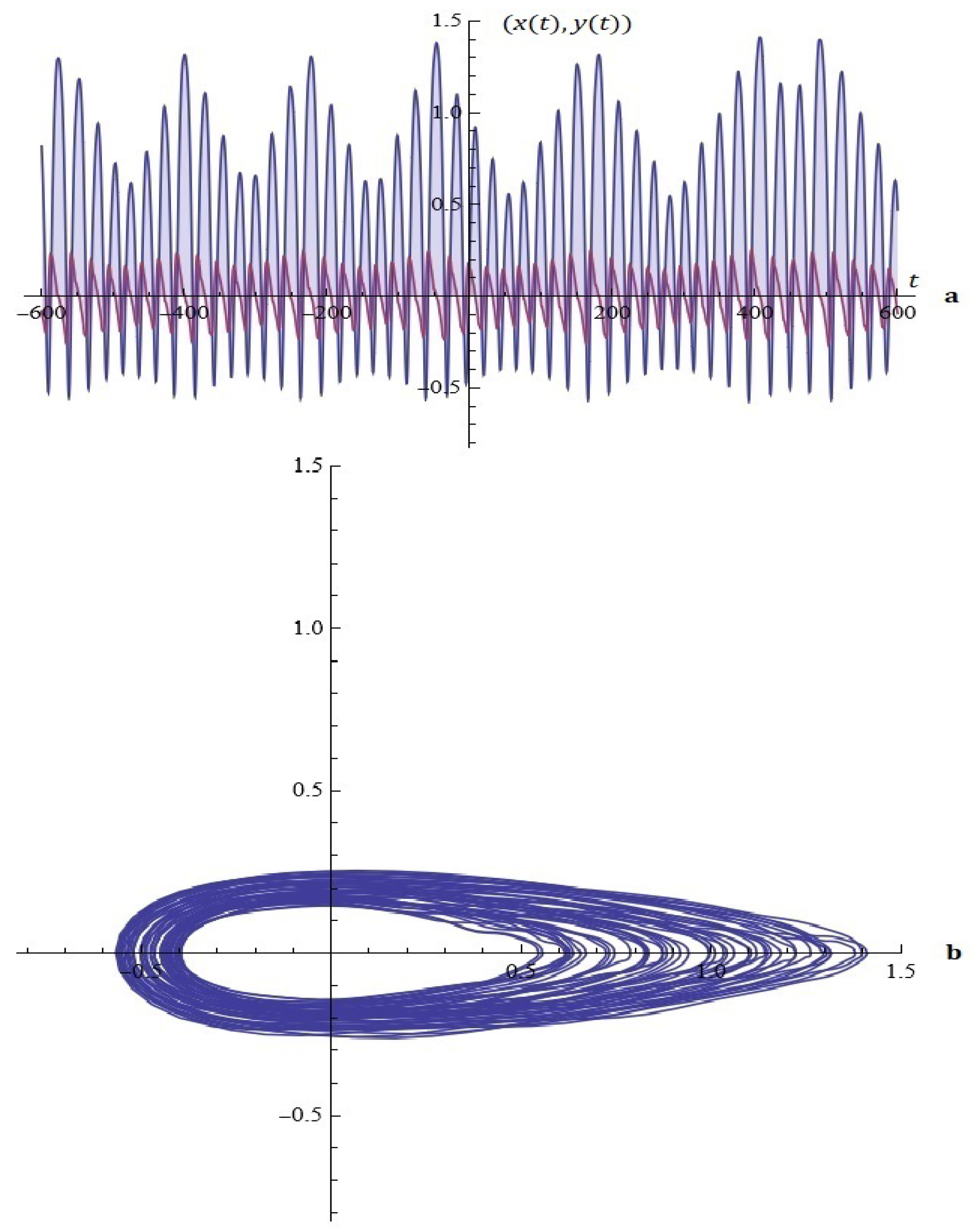
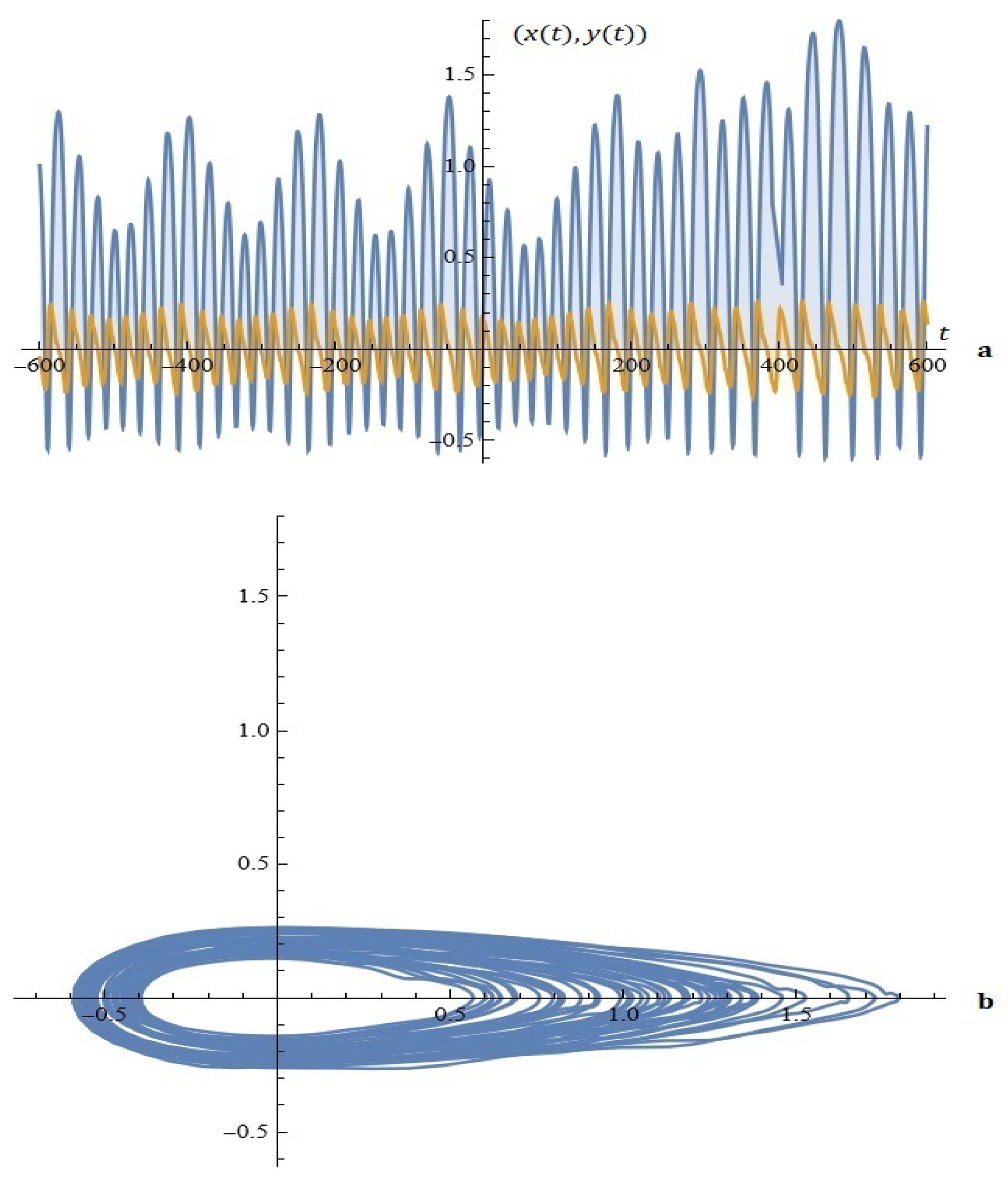
Example A1.
3. Finally, let us discuss Model B under the assumptions of Section 2.1.2. Dynamics (9) can be written as
The examples provided in Section 2.1.2 can be viewed in Figure A3—the new parameter P is assumed to be .

Figure A1.
(a) The Melnikov function. (b) A typical Melnikov antenna array.
Figure A1.
(a) The Melnikov function. (b) A typical Melnikov antenna array.
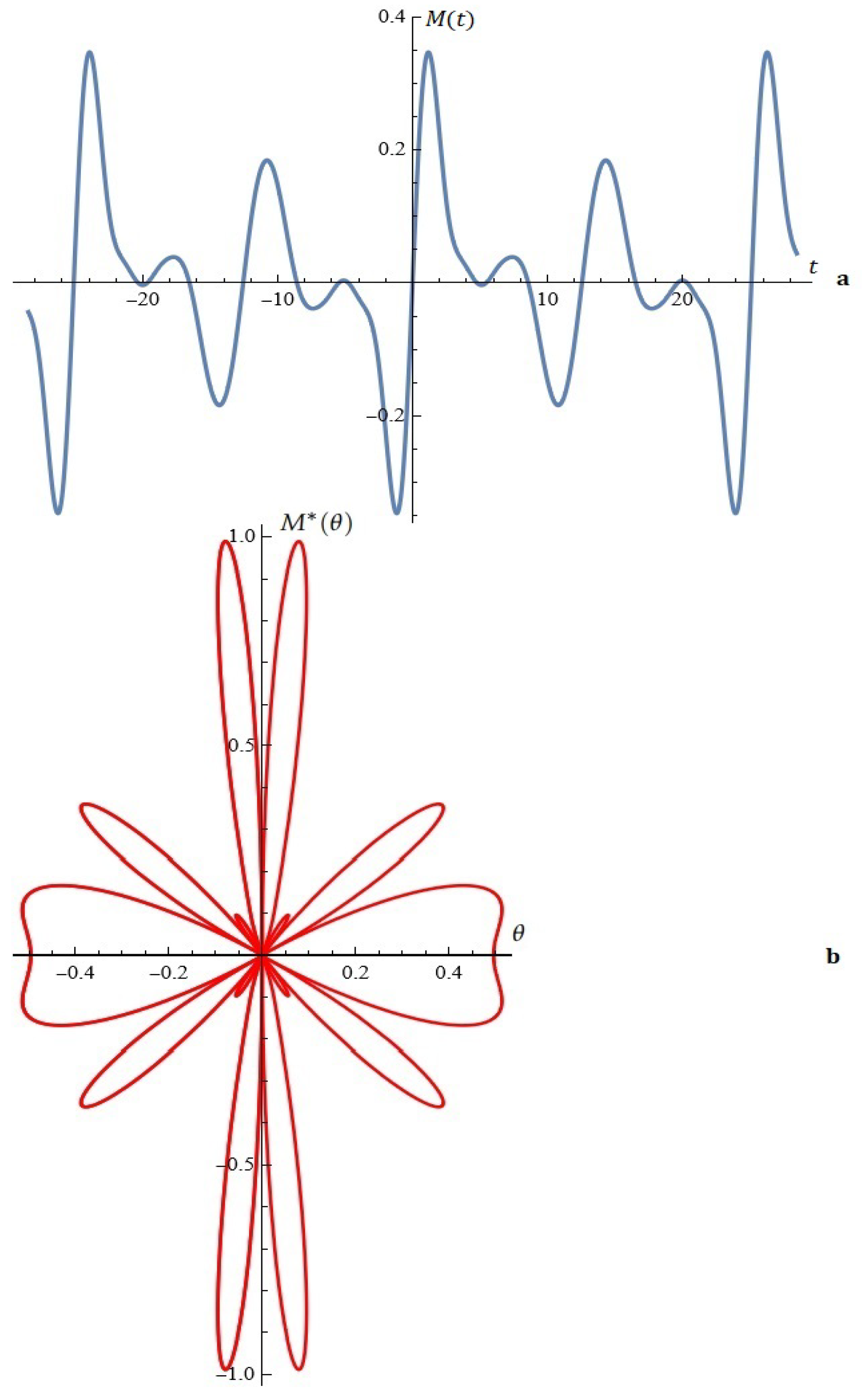
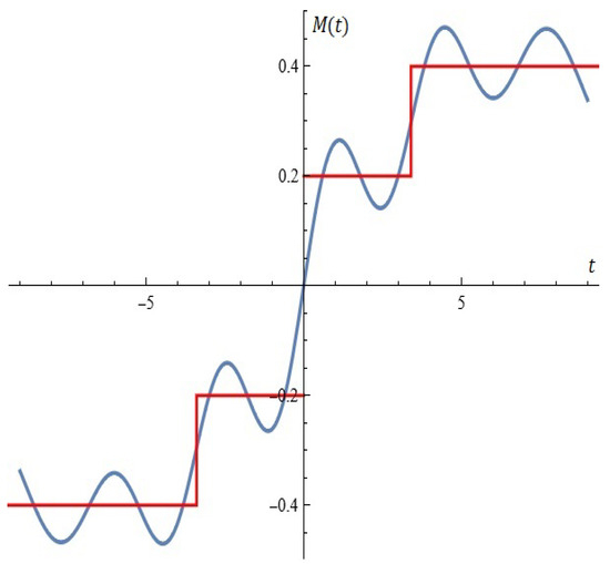
Figure A2.
A good approximation of the electrical stage by Melnikov function (Example 2).
Figure A2.
A good approximation of the electrical stage by Melnikov function (Example 2).
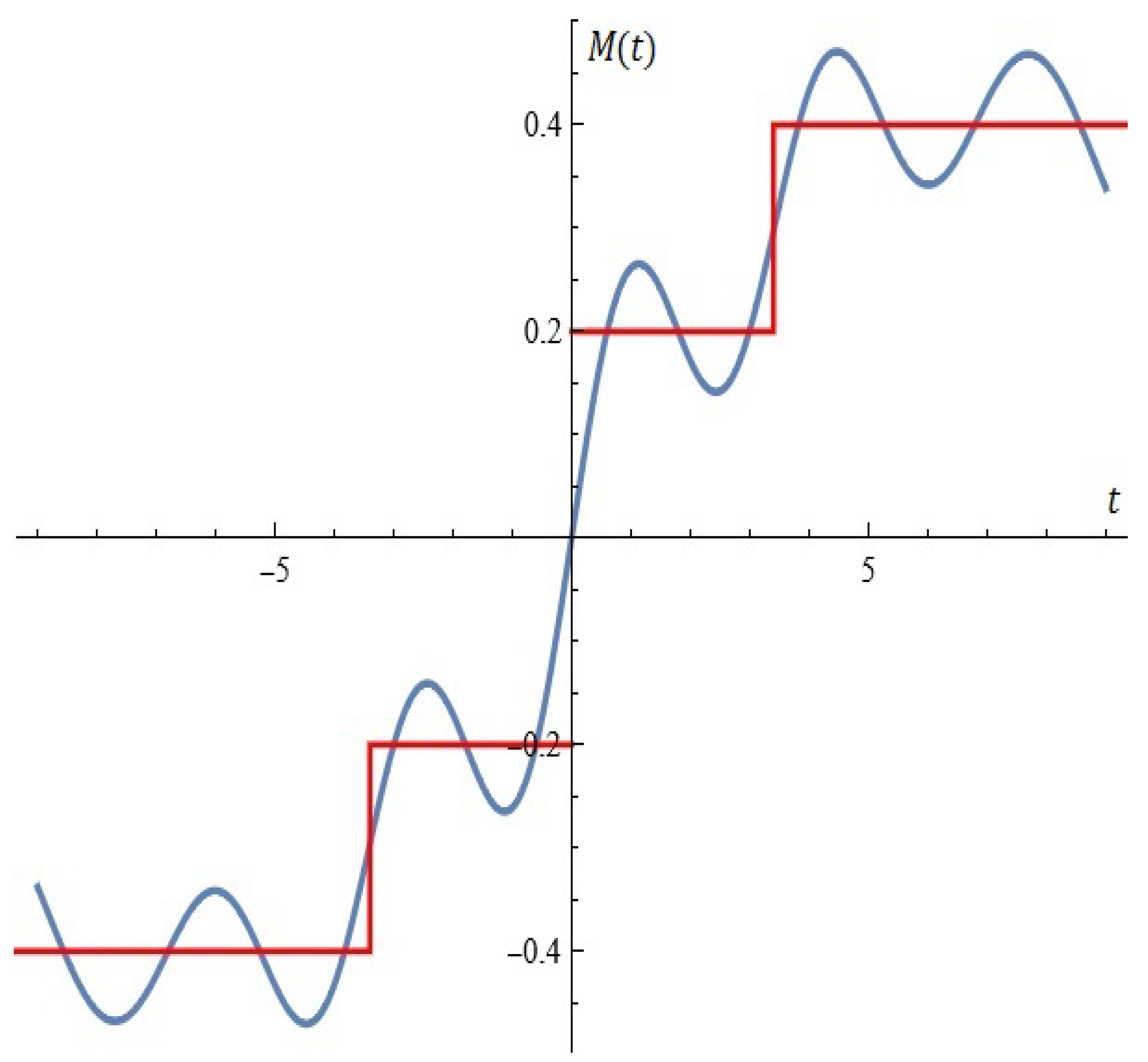
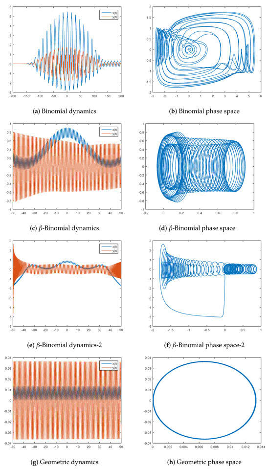
Figure A3.
Oscillators based on the binomial and -binomial distributions.
Figure A3.
Oscillators based on the binomial and -binomial distributions.
Thus, the Melnikov function and the related equation turns into
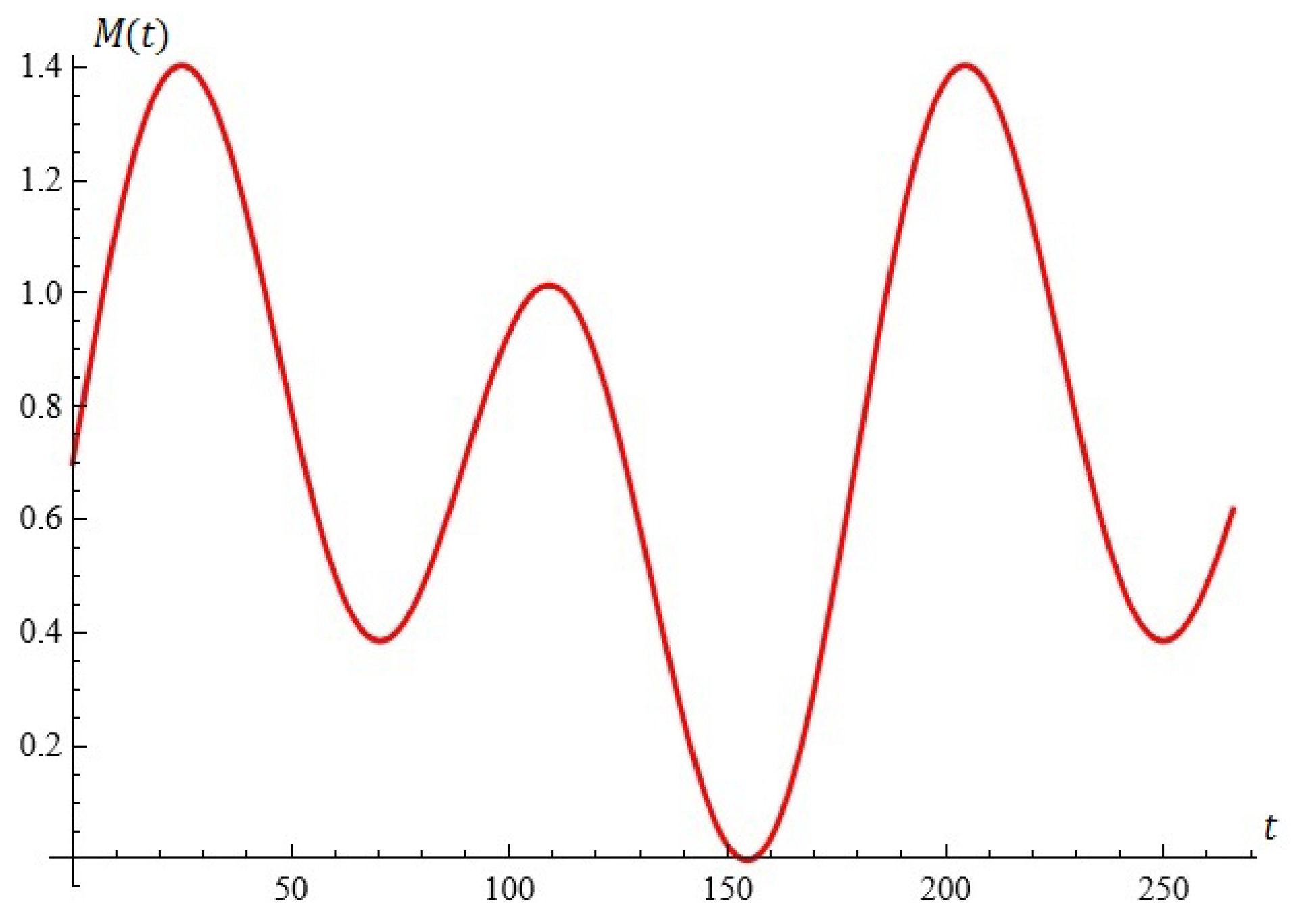
4. In a number of cases, the Melnikov function can be used to approximate electrical stages (see Figure A2).
Example A2.
Let , , , . A good approximation of the electrical stage by Melnikov function is depicted in Figure A2.
5. We note that Figure A2 actually depicts the approximation of the function:
In hidden form, a numerical method is used to explicitly calculate the Melnikov polynomial of the best uniform approximation. This algorithm is a modification of one of the methods of E. Remez. For some details, see [21].
Obviously, Melnikov polynomials can be used to approximate arbitrary point sets in the plane about uniform and Hausdorff metrics. Such tasks are relevant to the general theory of synthesis and the analysis of digital filters (see, for example, Refs. [22,23]). We will explicitly note that, with a special choice of model parameters, the generated Melnikov polynomial can be used to approximate some special classes of point sets in the plane.
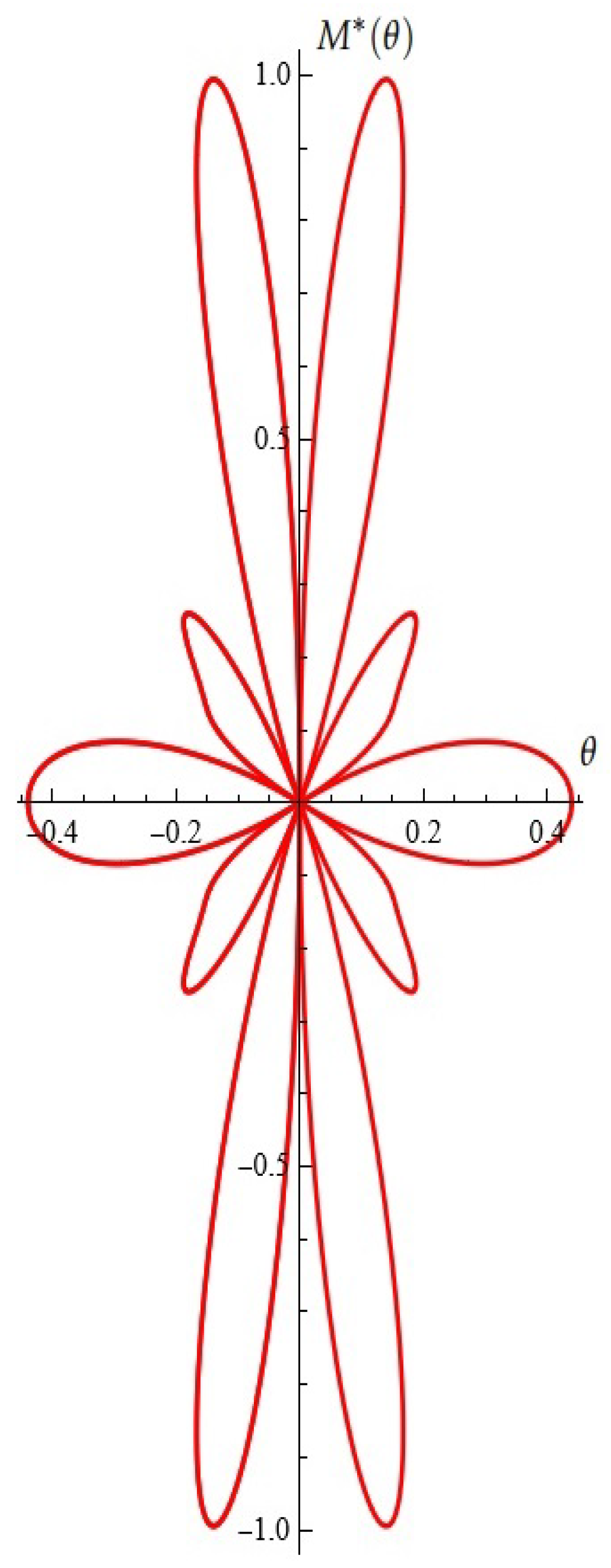
For example, a good approximation of the “Cross” point set is shown in Figure A4 above for fixed: , , .
This is a classic Akhiezer problem [24] for approximating the “Cross” point set with odd polynomials about uniform metrics and is important in the synthesis of so-called “difference radiation diagrams” (see, for example, Ref. [25]).

Figure A4.
A good approximation of the “Cross” point set.
Figure A4.
A good approximation of the “Cross” point set.
6. The general N-element linear phased array factor used to find coefficients is
where , d is element separation, is polar angle, and , where is a design parameter. This idea was borrowed from [19] in its generation of new Gegenbauer-like and Jacobi-like antenna arrays.
Of course, this relatively new idea of justification and right to exist is subject to serious research by specialists working in this scientific direction.
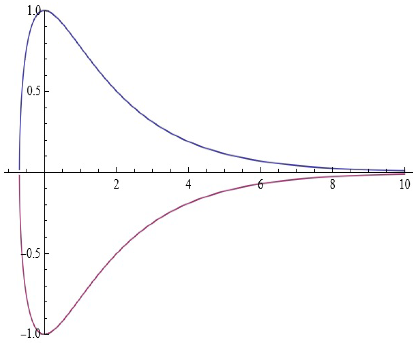
7. Let us discuss briefly some relations with the Proportional–Integral–Derivative (PID) controllers. The x-impact of in the y-dynamics comes from a function . Having in mind its derivative, , we conclude that the function starts at the minus infinity, increases before (the value is ), and then decreases to zero. Its unique root is achieved for . This shape indicates the following behavior of our models. If the function falls enough below zero, then the negative coefficient shoots up the y-part. Thus, the x-dynamics slows its fall (if y is still negative), changing the trend, or increases faster (if y is positive). The inverse circumstances describe the model dynamics when is positive.
8. For several control strategies to stabilize the chaotic behavior of a fractional piecewise-smooth oscillator, see [26].
9. Important issues related to the study of analytical predictions of Melnikov chaos through the visualization of basins of attraction, bifurcation diagrams, Lyapunov exponents, and Poincaré sections will be investigated in our future work.
References
- Krajnak, V.; Wiggins, S. Dynamics of the Morse oscillator: Analytical expressions for trajectories, action–angle variables, and chaos dynamics. arXiv 2019, arXiv:1905.04059V1. [Google Scholar]
- Morse, P. Diatomic molecules according to the wave mechanics. II. Vibrational levels. Phys. Rev. 1929, 34, 57–64. [Google Scholar] [CrossRef]
- Wiggins, S. Introduction to Applied Nonlinear Dynamical Systems and Chaos; Springer: Berlin, Germany, 1990. [Google Scholar]
- Mezic, I.; Wiggnis, S. On the integrability and perturbation of three–dimensional fluid flows with symmetry. J. Nonlinear Sci. 1994, 4, 157–194. [Google Scholar] [CrossRef]
- Goggin, M.; Milonni, P. Driven Morse oscillator: Classical chaos, quantum theory, and photodissociation. Phys. Rev. A 1988, 37, 796–806. [Google Scholar] [CrossRef]
- Bruhn, B. Homoclinic bifurcations in simple parametrically driven systems. Annalen der Physik 1989, 501, 367–375. [Google Scholar] [CrossRef]
- Melnikov, V. On the stability of the center for time periodic perturbations. Trans. Mosc. Math. Soc. 1963, 12, 1–57. [Google Scholar]
- Schecter, S. Persistent unstable equilibria and closed orbits of a singularly perturbed system. J. Differ. Equ. 1985, 60, 131–141. [Google Scholar] [CrossRef]
- McGehee, R. A stable manifold theorem for degenerate fixed point with applications to celestial mechanics. J. Differ. Equ. 1973, 14, 70–88. [Google Scholar] [CrossRef]
- Van Ek, K. The Homoclinic Melnikov Method. Ph.D. Thesis, University of Groningen, Groningen, The Netherlands, 2015. [Google Scholar]
- Golev, A.; Terzieva, T.; Iliev, A.; Rahnev, A.; Kyurkchiev, N. Simulation on a Generalized Oscillator Model: Web-Based Application. Comptes Rendus L’Academie Bulg. Des Sci. 2024, 77, 230–237. [Google Scholar] [CrossRef]
- Vasileva, M.; Kyurkchiev, V.; Iliev, A.; Rahnev, A.; Zaevski, T.; Kyurkchiev, N. Some Investigations and Simulations on the Generalized Rayleigh Systems, Duffing Systems with Periodic Parametric Excitation, Mathieu and Hopf Oscillators; Plovdiv University Press: Plovdiv, Bulgaria, 2024. [Google Scholar]
- Kyurkchiev, N.; Zaevski, T.; Iliev, A.; Kyurkchiev, V.; Rahnev, A. Nonlinear dynamics of a new class of micro-electromechanical oscillators–open problems. Symmetry 2024, 16, 253. [Google Scholar] [CrossRef]
- Kyurkchiev, N.; Zaevski, T.; Iliev, A.; Kyurkchiev, V.; Rahnev, A. Modeling of Some Classes of Extended Oscillators: Simulations, Algorithms, Generating Chaos, Open Problems. Algorithms 2024, 17, 121. [Google Scholar] [CrossRef]
- Xing, Q. Maslov index for heteroclinic orbits of non-Hamiltonian systems on a two-dimensional phase space. Topol. Methods Nonlinear Anal. 2022, 59, 113–130. [Google Scholar]
- Li, X. Limit cycles in a quartic system with a third-order nilpotent singular point. Adv. Differ. Equ. 2018, 2018, 152. [Google Scholar] [CrossRef]
- Li, F.; Liu, Y.; Liu, Y.; Yu, P. Bi-center problem and bifurcation of limit cycles from nilpotent singular points in Z2-equivariant cubic vector fields. J. Differ. Equ. 2018, 265, 4965–4992. [Google Scholar] [CrossRef]
- Kyurkchiev, N.; Andreev, A. Approximation and Antenna and Filters Synthesis. Some Moduli in Programming Environment MATHEMATICA; LAP LAMBERT Academic Publishing: Saarbrucken, Germany, 2014. [Google Scholar]
- Soltis, J. New Gegenbauer–like and Jacobi–like polynomials with applications. J. Frankl. Inst. 1993, 33, 635–639. [Google Scholar] [CrossRef]
- Iliev, A.; Kyurkchiev, N. Nontrivial Methods in Numerical Analysis: Selected Topics in Numerical Analysis; LAP LAMBERT Academic Publishing: Saarbrucken, Germany, 2010. [Google Scholar]
- Sendov, B.; Andreev, A. Approximation and interpolation theory. In Handbook of Numerical Analysis; Ciarlet, P., Lions, J., Eds.; Elsevier Science B. V.: Amsterdam, The Netherlands, 1994; Volume III. [Google Scholar]
- Apostolov, P. General theory, approximation method and design of electrical filters based on Hausdorff polynomials. Mech. Transp. Commun. 2007, 2, 1–8. [Google Scholar]
- Kyurkchiev, N. Some Intrinsic Properties of Tadmor–Tanner Functions: Related Problems and Possible Applications. Mathematics 2020, 8, 1963. [Google Scholar] [CrossRef]
- Akhiezer, N. Theory of Approximation, 2nd ed.; Nauka: Moskow, Russia, 1965. (In Russian) [Google Scholar]
- Kyurkchiev, N. Synthesis of Slot Aerial Grids with Hausdorff Type Directive Patterns. Ph.D. Thesis, Department of Radio-Electronics, VMEI, Sofia, Bulgaria, 1979. (In Bulgarian). [Google Scholar]
- Zhang, Y.; Li, J.; Zhu, S.; Zhao, H. Chaos detection and control of a fractional piecewise-smooth system with nonlinear damping. Chin. J. Phys. 2024, 90, 885–900. [Google Scholar] [CrossRef]


Disclaimer/Publisher’s Note: The statements, opinions and data contained in all publications are solely those of the individual author(s) and contributor(s) and not of MDPI and/or the editor(s). MDPI and/or the editor(s) disclaim responsibility for any injury to people or property resulting from any ideas, methods, instructions or products referred to in the content. |
© 2024 by the authors. Licensee MDPI, Basel, Switzerland. This article is an open access article distributed under the terms and conditions of the Creative Commons Attribution (CC BY) license (https://creativecommons.org/licenses/by/4.0/).