Two-Step Fifth-Order Efficient Jacobian-Free Iterative Method for Solving Nonlinear Systems

Abstract

This article introduces a novel two-step fifth-order Jacobian-free iterative method aimed at efficiently solving systems of nonlinear equations. The method leverages the benefits of Jacobian-free approaches, utilizing divided differences to circumvent the computationally intensive calculation of Jacobian matrices. This adaptation significantly reduces computational overhead and simplifies the implementation process while maintaining high convergence rates. We demonstrate that this method achieves fifth-order convergence under specific parameter settings, with broad applicability across various types of nonlinear systems. The effectiveness of the proposed method is validated through a series of numerical experiments that confirm its superior performance in terms of accuracy and computational efficiency compared to existing methods.

1. Introduction

Let $F\left(x\right)=0$ be a nonlinear system of equations, $F:D\subset {\mathbb{R}}^n\to {\mathbb{R}}^n$, and the functions $f_i$ for $i=1,2,\dots ,n$ be the coordinate components of F, expressed as $F\left(x\right)={\left(f_1\left(x\right),f_2\left(x\right),\dots ,f_n\left(x\right)\right)}^T$. Solving nonlinear systems is generally challenging, and solutions $\xi$ are typically found by linearizing the problem or employing a fixed-point iteration function $G:D\subset {\mathbb{R}}^n\to {\mathbb{R}}^n$, leading to an iterative fixed-point method. Among the various root-finding techniques for nonlinear systems, Newton’s method is the most well known, and follows the second-order iterative procedure:

$$x^{(k+1)}=x^{\left(k\right)}-{\left[F^{\prime }\left(x^{\left(k\right)}\right)\right]}^{-1}F\left(x^{\left(k\right)}\right),k=0,1,\dots ,$$

$F^{\prime }\left(x^{\left(k\right)}\right)$ being the Jacobian matrix of F at the k-th iterate.

Recently, many researchers have focused on developing iterative methods that outperform Newton’s method in terms of both efficiency and order of convergence. Numerous approaches need the computation of $F^{\prime }$ at different points along each iteration. Nevertheless, calculating the Jacobian poses significant challenges, particularly in high-dimensional problems, where its computation can be costly or even impractical (see for an example [1,2,3,4,5] and the references therein). In some instances, the Jacobian may not exist at all. To address this issue, alternative approaches have been proposed in the literature, such as replacing the Jacobian matrix with a divided difference operator. One of the simplest alternatives is the multidimensional version of Steffensen’s method, attributed to Samanskii [6,7], which substitutes the Jacobian in Newton’s procedure with a first-order operator of divided differences:

$$x^{(k+1)}=x^{\left(k\right)}-{[x^{\left(k\right)},z^{\left(k\right)};F]}^{-1}F\left(x^{\left(k\right)}\right),k=0,1,\dots ,$$

where $z^{\left(k\right)}=x^{\left(k\right)}+F\left(x^{\left(k\right)}\right)$, and $[·,·;F]:\mathsf{\Omega }\times \mathsf{\Omega }\subset {\mathbb{R}}^n\times {\mathbb{R}}^n\to \mathcal{L}\left({\mathbb{R}}^n\right)$ is the operator of divided differences related to F [8],

$$[y,x;F](y-x)=F\left(y\right)-F\left(x\right) \mathrm{for\; any} x,y\in \mathsf{\Omega }.$$

The implementation of this divided difference is carried out, for all $1\le i,j\le n$, as

$${[y,x;F]}_{i,j}={\displaystyle \frac{F_i(y_1,y_2,\dots ,y_{j-1},y_j,x_{j+1},\dots ,x_n)-F_i(y_1,y_2,\dots ,y_{j-1},x_j,x_{j+1},\dots ,x_n)}{y_j-x_j}},$$

where $x={(x_1,x_2,\dots ,x_{j-1},x_j,x_{j+1},\dots ,x_n)}^T$ and $y={(y_1,y_2,\dots ,y_{j-1},y_j,y_{j+1},\dots ,y_n)}^T$, as defined by Ortega et al. in [8]. This substitution retains the second order of convergence while bypassing the calculation of $F^{\prime }$. However, the set of converging initial estimations is dramatically reduced by this replacement in case of Newton’s and Samanskii’s schemes. This implies that the initial estimation used in the iterative procedures must be closer to the (unknown) solution in order to converge. This Jacobian-free scheme is known as an unstable variant of Newton’s procedure.

Although both the Samanskii and Newton methods exhibit quadratic convergence, it has been shown that the Jacobian-free scheme is less stable than Newton’s method, with stability depending more on the initial guess. This has been thoroughly analyzed in [9,10,11,12,13], where it was found that, for scalar cases $f\left(x\right)=0$, derivative-free iterative methods become more stable when selecting $z=x+\alpha f\left(x\right)$ for small real values of $\alpha$.

Our aim in this manuscript is to propose a very efficient and stable class of Jacobian-free iterative methods. Its convergence order is fourth, although it holds a fifth-order element. The main achievement of this construction is the relation between scalar accelerators, firstly appearing in [14], with the vectorial point-wise power weight function introduced firstly in [15]. The first technique allows faster convergence with low computational costs, while the second one improves the stability of Jacobian-free methods, allowing convergence to the solution with initial estimations that are not so close to the solution as in Samanskii’s case. These techniques are presented in the following state of the art, showing some of the advances in this specific area of research in the last few years.

However, substituting the Jacobian with divided differences can result in a lower convergence order for some iterative methods, for example the multidimensional version of Ostrowski’s fourth-order method (see [16]),

$$\begin{array}{cc}\hfill y^{\left(k\right)}& =x^{\left(k\right)}-{\left[F^{\prime }\left(x^{\left(k\right)}\right)\right]}^{-1}F\left(x^{\left(k\right)}\right),\hfill \\ \hfill x^{(k+1)}& =y^{\left(k\right)}-{\left[2[y^{\left(k\right)},x^{\left(k\right)};F]-F^{\prime }\left(x^{\left(k\right)}\right)\right]}^{-1}F\left(y^{\left(k\right)}\right),k=0,1,\dots ,\hfill \end{array}$$

achieves only cubic convergence if $F^{\prime }\left(x\right)$ is replaced by $[y,x;F]$, as follows:

$$\begin{array}{cc}\hfill y^{\left(k\right)}& =x^{\left(k\right)}-{[x^{\left(k\right)}+F\left(x^{\left(k\right)}\right),x^{\left(k\right)};F]}^{-1}F\left(x^{\left(k\right)}\right),k=0,1,\dots ,\hfill \\ \hfill x^{(k+1)}& =y^{\left(k\right)}-{\left[2[y^{\left(k\right)},x^{\left(k\right)};F]-[x^{\left(k\right)}+F\left(x^{\left(k\right)}\right),x^{\left(k\right)};F]\right]}^{-1}F\left(y^{\left(k\right)}\right).\hfill \end{array}$$

Despite the reduction in performance observed in some Jacobian-free methods, it is important to highlight that there are iterative methods that are successfully modified in their iterative expressions to preserve the order of convergence, even after fully transiting to Jacobian-free formulations. This is the case of a combination of the Traub–Steffensen family of methods and a second step with divided difference operators, proposed by Behl et al. in [17].

$$\begin{array}{cc}\hfill y^{\left(k\right)}& =x^{\left(k\right)}-{\left[u^{\left(k\right)},x^{\left(k\right)};F\right]}^{-1}F\left(x^{\left(k\right)}\right),k=0,1,2,\dots \hfill \\ \hfill x^{(k+1)}& =y^{\left(k\right)}-{\left[y^{\left(k\right)},x^{\left(k\right)};F\right]}^{-1}\left[u^{\left(k\right)},x^{\left(k\right)};F\right]{\left[u^{\left(k\right)},y^{\left(k\right)};F\right]}^{-1}F\left(y^{\left(k\right)}\right),\hfill \end{array}$$

(1)

where $u^{\left(k\right)}=x^{\left(k\right)}+\beta F\left(x^{\left(k\right)}\right),\beta \in \mathbb{R}$. The iterative schemes have a fourth order of convergence for every $\beta$, $\beta \ne 0$; for our purposes, we choose $\beta =1$, and this is called Traub-Ste. Let us remark that different approximations of the Jacobian matrix have been necessary to hold the original order of convergence, increasing the computational cost and, therefore, diminishing its efficiency.

Other fourth-order methods also lose their convergence order when the Jacobian is replaced with divided differences, such as Jarratt’s scheme [18], Sharma’s method [19], Montazeri’s method [20], Ostrowski’s vectorial extension ([16]), and Sharma–Arora’s fifth-order scheme [21]. In all these cases, Jacobian-free versions of the methods reduce to lower orders of convergence. Nevertheless, Amiri et al. [15] demonstrated that using a specialized divided difference operator of the form $[x,x+G(x);F]$, where $G\left(x\right)={\left(f_1{\left(x\right)}^m,f_2{\left(x\right)}^m,\dots ,f_n{\left(x\right)}^m\right)}^T$, $m\in \mathbb{N}$, as an approximation of the Jacobian matrix may preserve the convergence order. By selecting an appropriate parameter m, the original fourth-order convergence of these methods can be maintained. Also, the appropriate value of m for each optimal order of convergence was conjectured.

For the sake of comparison with our proposed methods, we now consider several efficient vectorial iterative schemes existing in the literature to be transformed into their Jacobian-free versions following the idea of Amiri et al. [15]. This technique allowed us to design Jacobian-free partners of vectorial schemes with minimal computational costs. In the efficiency and numerical sections, we compare these Jacobian-free schemes with our proposed procedures. The first one is the vectorial extension of Ostrowski’s scheme (see [16,22], for instance),

$$\begin{array}{cc}\hfill y^{\left(k\right)}& =x^{\left(k\right)}-{\left[F^{\prime }\left(x^{\left(k\right)}\right)\right]}^{-1}F\left(x^{\left(k\right)}\right),\hfill \\ \hfill x^{(k+1)}& =y^{\left(k\right)}-{\left[2\left[y^{\left(k\right)},x^{\left(k\right)};F\right]-F^{\prime }\left(x^{\left(k\right)}\right)\right]}^{-1}F\left(y^{\left(k\right)}\right),\hfill \end{array}$$

(2)

whose Jacobian-free version, obtained by substituting the Jacobian matrix by the divided difference operator (with Amiri et al. approach [15], $m=2$), is

$$\begin{array}{cc}\hfill y^{\left(k\right)}& =x^{\left(k\right)}-{\left[u^{\left(k\right)},x^{\left(k\right)};F\right]}^{-1}F\left(x^{\left(k\right)}\right),\hfill \\ \hfill x^{(k+1)}& =y^{\left(k\right)}-{\left[2\left[y^{\left(k\right)},x^{\left(k\right)};F\right]-\left[u^{\left(k\right)},x^{\left(k\right)};F\right]\right]}^{-1}F\left(y^{\left(k\right)}\right),\hfill \end{array}$$

(3)

where $\left[u^{\left(k\right)},x^{\left(k\right)},F\right]\approx F^{\prime }\left(x^{\left(k\right)}\right)$, and $u^{\left(k\right)}=x^{\left(k\right)}+\alpha G\left(x^{\left(k\right)}\right)$ (with $m=2$), $\alpha \in \mathbb{R}$. We denote this method as $Ostr{o}_{01}$.

Another fourth-order method proposed by Sharma in [19] using Jacobian matrices is

$$\begin{array}{cc}\hfill y^{\left(k\right)}& =x^{\left(k\right)}-{\left[F^{\prime }\left(x^{\left(k\right)}\right)\right]}^{-1}F\left(x^{\left(k\right)}\right),\hfill \\ \hfill x^{(k+1)}& =y^{\left(k\right)}-\left[3I-2{\left[F^{\prime }\left(x^{\left(k\right)}\right)\right]}^{-1}[y^{\left(k\right)},x^{\left(k\right)};F]\right]{\left[F^{\prime }\left(x^{\left(k\right)}\right)\right]}^{-1}F\left(y^{\left(k\right)}\right),\hfill \end{array}$$

(4)

to which we apply the same procedure, Amiri’s, performed for (2), obtaining its Jacobian-free partner

$$\begin{array}{cc}\hfill y^{\left(k\right)}& =x^{\left(k\right)}-{\left[u^{\left(k\right)},x^{\left(k\right)};F\right]}^{-1}F\left(x^{\left(k\right)}\right),\hfill \\ \hfill x^{(k+1)}& =y^{\left(k\right)}-\left[3I-2{\left[u^{\left(k\right)},x^{\left(k\right)};F\right]}^{-1}[y^{\left(k\right)},x^{\left(k\right)};F]\right]{\left[u^{\left(k\right)},x^{\left(k\right)};F\right]}^{-1}F\left(y^{\left(k\right)}\right),\hfill \end{array}$$

(5)

which we denote by $M_{4,3}$, $\left[u^{\left(k\right)},x^{\left(k\right)},F\right]\approx F^{\prime }\left(x^{\left(k\right)}\right)$ and $u^{\left(k\right)}=x^{\left(k\right)}+\alpha G\left(x^{\left(k\right)}\right)$, $m=2$, first appeared in [15].

We finish with a sixth-order scheme [19], which is obtained by adding a step to the previous method (4),

$$\begin{array}{cc}\hfill y^{\left(k\right)}& =x^{\left(k\right)}-{\left[F^{\prime }\left(x^{\left(k\right)}\right)\right]}^{-1}F\left(x^{\left(k\right)}\right),k=0,1,\dots ,\hfill \\ \hfill z^{\left(k\right)}& =y^{\left(k\right)}-\left[3I-2{\left[F^{\prime }\left(x^{\left(k\right)}\right)\right]}^{-1}[y^{\left(k\right)},x^{\left(k\right)};F]\right]{\left[F^{\prime }\left(x^{\left(k\right)}\right)\right]}^{-1}F\left(y^{\left(k\right)}\right),\hfill \\ \hfill x^{(k+1)}& =z^{\left(k\right)}-\left[3I-2{\left[F^{\prime }\left(x^{\left(k\right)}\right)\right]}^{-1}[y^{\left(k\right)},x^{\left(k\right)};F]\right]{\left[F^{\prime }\left(x^{\left(k\right)}\right)\right]}^{-1}F\left(z^{\left(k\right)}\right).\hfill \end{array}$$

(6)

Similarly, its Jacobian-free version was constructed in [15] and denoted by $M_{6,3}$,

$$\begin{array}{cc}\hfill y^{\left(k\right)}& =x^{\left(k\right)}-{\left[u^{\left(k\right)},x^{\left(k\right)};F\right]}^{-1}F\left(x^{\left(k\right)}\right),k=0,1,\dots ,\hfill \\ \hfill z^{\left(k\right)}& =y^{\left(k\right)}-\left[3I-2{\left[u^{\left(k\right)},x^{\left(k\right)};F\right]}^{-1}[y^{\left(k\right)},x^{\left(k\right)};F]\right]{\left[u^{\left(k\right)},x^{\left(k\right)};F\right]}^{-1}F\left(y^{\left(k\right)}\right),\hfill \\ \hfill x^{(k+1)}& =z^{\left(k\right)}-\left[3I-2{\left[u^{\left(k\right)},x^{\left(k\right)};F\right]}^{-1}[y^{\left(k\right)},x^{\left(k\right)};F]\right]{\left[u^{\left(k\right)},x^{\left(k\right)};F\right]}^{-1}F\left(z^{\left(k\right)}\right).\hfill \end{array}$$

(7)

where again, $\left[u^{\left(k\right)},x^{\left(k\right)},F\right]\approx F^{\prime }\left(x^{\left(k\right)}\right)$ and $u^{\left(k\right)}=x^{\left(k\right)}+\alpha G\left(x^{\left(k\right)}\right)$, $m=2$. It should be noticed that in schemes (3), (5) and (7), a quadratic element-by-element power of $F\left(x^{\left(k\right)}\right)$ was employed in the divided differences. This adjustment was essential for preserving the convergence order of the original method (see [15]). However, in our proposal, the order of convergence of the original schemes is held, avoiding the computational cost of this element-by-element power.

Therefore, we aim to avoid the calculation of Jacobian matrices, which can be a bottleneck in terms of computational efficiency, especially for large systems. To achieve this, we present a two-step fifth-order efficient Jacobian-free iterative method that addresses these challenges by eliminating the need for direct Jacobian computation. Our approach is grounded in the use of divided differences and scalar accelerators recently developed in some very efficient schemes (using Jacobian matrices) [14,23]. This not only reduces the computational costs, but also accelerates the convergence with simpler iterative expressions. The proposed method’s design and theoretical underpinnings are discussed, emphasizing its ability to achieve high-order convergence without the Jacobian calculations typically required.

Our proposal is a variant of the scheme proposed by Singh, Sharma and Kumar in [14],

$$\begin{array}{cc}\hfill w^{\left(k\right)}& =x^{\left(k\right)}-F^{\prime }{\left(x^{\left(k\right)}\right)}^{-1}F\left(x^{\left(k\right)}\right),k=0,1,2,\dots \hfill \\ \hfill x^{(k+1)}& =w^{\left(k\right)}-\left(p_1+p_2{\displaystyle \frac{F{\left(w^{\left(k\right)}\right)}^{T}F\left(w^{\left(k\right)}\right)}{F{\left(x^{\left(k\right)}\right)}^{T}F\left(x^{\left(k\right)}\right)}}\right)F^{\prime }{\left(w^{\left(k\right)}\right)}^{-1}F\left(w^{\left(k\right)}\right),\hfill \end{array}$$

(8)

where ${\displaystyle \frac{F{\left(y^{\left(k\right)}\right)}^{T}F\left(y^{\left(k\right)}\right)}{F{\left(x^{\left(k\right)}\right)}^{T}F\left(x^{\left(k\right)}\right)}}$ is a scalar accelerator that can be interpreted as $F{\left(y^{\left(k\right)}\right)}^{T}F\left(y^{\left(k\right)}\right)={\parallel F\left(y^{\left(k\right)}\right)\parallel }^2$, and $F{\left(x^{\left(k\right)}\right)}^{T}F\left(x^{\left(k\right)}\right)={\parallel F\left(x^{\left(k\right)}\right)\parallel }^2$, respectively. The real parameters $p_1$ and $p_2$ make the order of convergence of the method five if $p_1$ = $p_2=1$, the order four if $p_1=1$ and $p_2$ is arbitrary, and the order two if $p_1\ne 1$ and $p_2$ is arbitrary. It is known that in many practical applications, computing the Jacobian matrix can be very resource-intensive and time-consuming; therefore, Jacobian-free methods are often preferred.

Making a modification to the scheme (8) by replacing the Jacobian matrices by specific divided differences, we obtain the following family of novel Jacobian-free methods:

$$\begin{array}{cc}\hfill y^{\left(k\right)}& =x^{\left(k\right)}-{\left[u_x^{\left(k\right)},x^{\left(k\right)},F\right]}^{-1}F\left(x^{\left(k\right)}\right),k=0,1,2,\dots \hfill \\ \hfill x^{(k+1)}& =y^{\left(k\right)}-\left(p_1+p_2{\displaystyle \frac{F{\left(y^{\left(k\right)}\right)}^{T}F\left(y^{\left(k\right)}\right)}{F{\left(x^{\left(k\right)}\right)}^{T}F\left(x^{\left(k\right)}\right)}}\right){\left[u_y^{\left(k\right)},y^{\left(k\right)},F\right]}^{-1}F\left(y^{\left(k\right)}\right),\hfill \end{array}$$

(9)

where $\left[u_x^{\left(k\right)},x^{\left(k\right)};F\right]\approx F^{\prime }\left(x^{\left(k\right)}\right)$, $\left[u_y^{\left(k\right)},y^{\left(k\right)};F\right]\approx F^{\prime }\left(y^{\left(k\right)}\right)$, $u_x^{\left(k\right)}=x^{\left(k\right)}+\alpha F\left(x^{\left(k\right)}\right)$ and $u_y^{\left(k\right)}=y^{\left(k\right)}+\alpha F\left(y^{\left(k\right)}\right)$. From now on, we will refer to our modified scheme as $MS(p_1,p_2)$. This class of iterative schemes uses scalar accelerators, in order to achieve high-order convergence with low computational effort, and also obtains good stability properties by using vectorial point-wise weight functions in the first-order divided differences. These properties have, as a direct consequence, higher efficiency compared with the existing Jacobian-free methods previously mentioned, as well as good numerical results on nonlinear systems of different sizes.

In Section 2, we demonstrate the theoretical order of convergence of the new parametric class of Jacobian-free iterative methods using scalar accelerators, depending on the values of the parameters involved. Subsequently, in Section 3 we carry out an efficiency analysis in which we compare our proposed method with the Jacobian-free versions of others previously cited in the literature, with excellent results. Finally, Section 4 presents practical results of these iterative methods applied to different nonlinear systems of equations, the testing of which confirms the theoretical results for both small- and big-sized academical and applied systems.

2. Convergence of New Jacobian-Free Iterative Method

The following result shows the error equations arising from method (9) for the possible parameter values, thereby demonstrating that the convergence results of the family (8) hold.

Theorem 1.

Let F be a differentiable enough function $F:\mathsf{\Omega }\subseteq {\mathbb{R}}^n\to {\mathbb{R}}^n$, defined in the open convex neighborhood Ω of ξ solution of $F\left(x\right)=0$. Let us also consider an initial seed $x^{\left(0\right)}$ near enough to ξ and let $F^{\prime }\left(x\right)$ be continuous and invertible at ξ. Then, the parametric class of iterative schemes presented in (9) locally converges for all $\alpha \in \mathbb{R}$, with the order of convergence given by the following:

(a) 

Fifth-order convergence if $p_1=p_2=1$, the corresponding error equation being

$$\begin{array}{cc}\hfill x^{(k+1)}-\xi & =(M_4-A_2(M_2{M}_1+M_1{M}_2)-(C_1+C_2)M_2-((M_1^2+M_1)M_2+M_2{M}_1\hfill \\ \hfill & -P^{-1}{M}_1^{2}Q\left)M_1\right)e^{{\left(k\right)}^5}+O\left(e^{{\left(k\right)}^6}\right).\hfill \end{array}$$

(10)

(b) 

Fourth-order convergence if $p_1=1,p_2\ne 1$, the corresponding error equation being

$$\begin{array}{cc}\hfill x^{(k+1)}-\xi & =(-A_2{M}_1^2+C_1{M}_1-p_2{M}_1^3)e^{{\left(k\right)}^4}\hfill \\ \hfill & +(M_4-p_1(A_2(M_2{M}_1+M_1{M}_2)-(C_1+C_2)M_2)-\left(p_2\right((M_1^2+M_1)M_2\hfill \\ \hfill & +M_2{M}_1-P^{-1}{M}_1^{2}Q\left)M_1\right)e^{{\left(k\right)}^5}+O\left(e^{{\left(k\right)}^6}\right).\hfill \end{array}$$

(11)

(c) 

Second-order convergence if $p_1\ne 1,p_{2}arbitrary$, the corresponding error equation being

$$\begin{array}{cc}\hfill x^{(k+1)}-\xi & =M_1(1-p_1)e^{{\left(k\right)}^2}+M_2(1-p_1)e^{{\left(k\right)}^3}\hfill \\ \hfill & +(M_3(1-p_1)-p_1{A}_2{M}_1^2+p_1{C}_1{M}_1-p_2{M}_1^3)e^{{\left(k\right)}^4}\hfill \\ \hfill & +(M_4-p_1(A_2(M_2{M}_1+M_1{M}_2)-(C_1+C_2)M_2)-\left(p_2\right((M_1^2+M_1)M_2\hfill \\ \hfill & +M_2{M}_1-P^{-1}{M}_1^{2}Q\left)M_1\right)e^{{\left(k\right)}^5}+O\left(e^{{\left(k\right)}^6}\right),\hfill \end{array}$$

(12)

where $A_j={\displaystyle \frac{1}{j!}}{\left[F^{\prime }\left(\xi \right)\right]}^{-1}{F}^{\left(j\right)}\left(\xi \right)$, $j=2,3,\dots$, and $C_i,M_i$, $i=1,2,\dots$ are combinations of $A_j$, denoting the error at iteration k by $e^{\left(k\right)}=x^{\left(k\right)}-\xi$.

Proof. 

Let $e^{\left(k\right)}=x^{\left(k\right)}-\xi$ be the error at the k-th iteration and let $\xi \in {\mathbb{R}}^n$ be a solution of $F\left(x\right)=0$. Then, expanding $F\left(x^{\left(k\right)}\right)$ in the neighborhood of $\xi$, we have

$$\begin{array}{cc}\hfill F\left(x^{\left(k\right)}\right)& =F^{\prime }\left(\xi \right)\left[e^{\left(k\right)}+A_2{e}^{{\left(k\right)}^2}+A_3{e}^{{\left(k\right)}^3}+A_4{e}^{{\left(k\right)}^4}+A_5{e}^{{\left(k\right)}^5}+A_6{e}^{{\left(k\right)}^6}+O\left(e^{{\left(k\right)}^7}\right)\right],\hfill \\ \hfill F^{\prime }\left(x^{\left(k\right)}\right)& =F^{\prime }\left(\xi \right)\left[I+2A_2{e}^{\left(k\right)}+3A_3{e}^{{\left(k\right)}^2}+4A_4{e}^{{\left(k\right)}^3}+5A_5{e}^{{\left(k\right)}^4}+6A_6{e}^{{\left(k\right)}^5}+O\left(e^{{\left(k\right)}^6}\right)\right],\hfill \\ \hfill F^{\prime \prime }\left(x^{\left(k\right)}\right)& =F^{\prime }\left(\xi \right)\left[2A_2+6A_3{e}^{\left(k\right)}+12A_4{e}^{{\left(k\right)}^2}+20A_5{e}^{{\left(k\right)}^3}+30A_6{e}^{{\left(k\right)}^4}+O\left(e^{{\left(k\right)}^5}\right)\right],\hfill \\ \hfill F^{\prime \prime \prime }\left(x^{\left(k\right)}\right)& =F^{\prime }\left(\xi \right)\left[6A_3+24A_4{e}^{\left(k\right)}+60A_5{e}^{{\left(k\right)}^2}+120A_6{e}^{{\left(k\right)}^3}+O\left(e^{{\left(k\right)}^4}\right)\right],\hfill \\ \hfill F^{\left(iv\right)}\left(x^{\left(k\right)}\right)& =F^{\prime }\left(\xi \right)\left[24A_4+120A_5{e}^{\left(k\right)}+360A_6{e}^{{\left(k\right)}^2}+O\left(e^{{\left(k\right)}^3}\right)\right],\hfill \\ \hfill F^{\left(v\right)}\left(x^{\left(k\right)}\right)& =F^{\prime }\left(\xi \right)\left[120A_5+720A_6{e}^{\left(k\right)}+O\left(e^{{\left(k\right)}^2}\right)\right],\hfill \\ \hfill F^{\left(vi\right)}\left(x^{\left(k\right)}\right)& =F^{\prime }\left(\xi \right)\left[720A_6+O\left(e^{\left(k\right)}\right)\right].\hfill \end{array}$$

(13)

Then, based on the formula of Genochi and Hermite (see [8]), we have

$$\begin{array}{cc}\hfill \left[u_x^{\left(k\right)},x^{\left(k\right)};F\right]& =F^{\prime }\left(x^{\left(k\right)}\right)+{\displaystyle \frac{1}{2!}}{F}^{\prime \prime }\left(x^{\left(k\right)}\right)(u_x^{\left(k\right)}-x^{\left(k\right)})+{\displaystyle \frac{1}{3!}}{F}^{\prime \prime \prime }\left(x^{\left(k\right)}\right){(u_x^{\left(k\right)}-x^{\left(k\right)})}^2\hfill \\ \hfill & +{\displaystyle \frac{1}{4!}}{F}^{\left(iv\right)}\left(x^{\left(k\right)}\right){(u_x^{\left(k\right)}-x^{\left(k\right)})}^3+{\displaystyle \frac{1}{5!}}{F}^{\left(v\right)}\left(x^{\left(k\right)}\right){(u_x^{\left(k\right)}-x^{\left(k\right)})}^4\hfill \\ \hfill & +{\displaystyle \frac{1}{6!}}{F}^{\left(vi\right)}\left(x^{\left(k\right)}\right){(u_x^{\left(k\right)}-x^{\left(k\right)})}^5+O\left({(u_{x^{\left(k\right)}}-x^{\left(k\right)})}^6\right).\hfill \end{array}$$

(14)

Taking into account that $u_x^{\left(k\right)}-x^{\left(k\right)}=\alpha F\left(x^{\left(k\right)}\right)$, and performing a series expansion up to the fifth order, we obtain

$$\begin{array}{cc}\hfill {\alpha }^2{\left(F\left(x^{\left(k\right)}\right)\right)}^2& ={\alpha }^2{\left(F^{\prime }\left(\xi \right)\right)}^2{e}^{{\left(k\right)}^2}+\alpha [{\left(F^{\prime }\left(\xi \right)\right)}^2{A}_2+F^{\prime }\left(\xi \right)A_2{F}^{\prime }\left(\xi \right)]e^{{\left(k\right)}^3}\hfill \\ \hfill & +{\alpha }^2[{\left(F^{\prime }\left(\xi \right)\right)}^2{A}_3+F^{\prime }\left(\xi \right)A_2{F}^{\prime }\left(\xi \right)A_2+F^{\prime }\left(\xi \right)A_3{F}^{\prime }\left(\xi \right)]e^{{\left(k\right)}^4}\hfill \\ \hfill & +{\alpha }^2[{\left(F^{\prime }\left(\xi \right)\right)}^2{A}_4+F^{\prime }\left(\xi \right)A_2{F}^{\prime }\left(\xi \right)A_3+F^{\prime }\left(\xi \right)A_3{F}^{\prime }\left(\xi \right)A_2+F^{\prime }\left(\xi \right)A_4{F}^{\prime }\left(\xi \right)]e^{{\left(k\right)}^5}\hfill \\ \hfill & +O\left(e^{{\left(k\right)}^6}\right),\hfill \\ \\ \hfill {\alpha }^3{\left(F\left(x^{\left(k\right)}\right)\right)}^3& ={\alpha }^3{\left(F^{\prime }\left(\xi \right)\right)}^3{e}^{{\left(k\right)}^3}+{\alpha }^3[{\left(F^{\prime }\left(\xi \right)\right)}^3{A}_2+{\left(F^{\prime }\left(\xi \right)\right)}^2{A}_2{F}^{\prime }\left(\xi \right)+F^{\prime }\left(\xi \right)A_2{\left(F^{\prime }\left(\xi \right)\right)}^2]e^{{\left(k\right)}^4}\hfill \\ \hfill & +{\alpha }^3[{\left(F^{\prime }\left(\xi \right)\right)}^3{A}_3+{\left(F^{\prime }\left(\xi \right)\right)}^2{A}_2{F}^{\prime }\left(\xi \right)A_2+F^{\prime }\left(\xi \right)A_2{\left(F^{\prime }\left(\xi \right)\right)}^2{A}_2+{\left(F^{\prime }\left(\xi \right)\right)}^2{A}_3{F}^{\prime }\left(\xi \right)\hfill \\ \hfill & +F^{\prime }\left(\xi \right)A_2{F}^{\prime }\left(\xi \right)A_2{F}^{\prime }\left(\xi \right)+F^{\prime }\left(\xi \right)A_3{\left(F^{\prime }\left(\xi \right)\right)}^2]e^{{\left(k\right)}^5}+O\left(e^{{\left(k\right)}^6}\right),\hfill \\ \\ \hfill {\alpha }^4{\left(F\left(x^{\left(k\right)}\right)\right)}^4& ={\alpha }^4{\left(F^{\prime }\left(\xi \right)\right)}^4{e}^{{\left(k\right)}^4}+{\alpha }^4[{\left(F^{\prime }\left(\xi \right)\right)}^4{A}_2+{\left(F^{\prime }\left(\xi \right)\right)}^3{A}_2{F}^{\prime }\left(\xi \right)\hfill \\ \hfill & +{\left(F^{\prime }\left(\xi \right)\right)}^2{A}_2{\left(F^{\prime }\left(\xi \right)\right)}^2+F^{\prime }\left(\xi \right)A_2\left({\left(F^{\prime }\left(\xi \right)\right)}^3\right]e^{{\left(k\right)}^5}+O\left(e^{k^6}\right),\hfill \\ \\ \hfill {\alpha }^5{\left(F\left(x^{\left(k\right)}\right)\right)}^5& =\alpha {\left(F^{\prime }\left(\xi \right)\right)}^5{e}^{{\left(k\right)}^5}+O\left(e^{{\left(k\right)}^6}\right).\hfill \end{array}$$

(15)

By combining Formulas (13) and (15) in the Taylor series expansion (14), we obtain the following:

$$\begin{array}{cc}\hfill \left[u_x^{\left(k\right)},x^{\left(k\right)};F\right]& =F^{\prime }\left(\xi \right)\left[I+B_1{e}^k+B_2{e}^{{\left(k\right)}^2}+B_3{e}^{{\left(k\right)}^3}+B_4{e}^{{\left(k\right)}^4}+B_5{e}^{{\left(k\right)}^5}+O\left(e^{{\left(k\right)}^6}\right)\right],\hfill \end{array}$$

(16)

where

$$\begin{array}{cc}\hfill B_1& =2A_2+\alpha A_2{F}^{\prime }\left(\xi \right),\hfill \\ \hfill B_2& =3A_3+\alpha A_2{F}^{\prime }\left(\xi \right)A_2+3\alpha A_3{F}^{\prime }\left(\xi \right)+{\alpha }^2{A}_3{\left(F^{\prime }\left(\xi \right)\right)}^2,\hfill \\ \hfill B_3& =4A_4+\alpha A_2{F}^{\prime }\left(\xi \right)A_3+3\alpha A_3{F}^{\prime }\left(\xi \right)A_2+6\alpha A_4{F}^{\prime }\left(\xi \right)+{\alpha }^2{A}_3{\left(F^{\prime }\left(\xi \right)\right)}^2{A}_2\hfill \\ \hfill & +{\alpha }^2{A}_3{F}^{\prime }\left(\xi \right)A_2{F}^{\prime }\left(\xi \right)+{\alpha }^{2}4A_4{\left(F^{\prime }\left(\xi \right)\right)}^2+{\alpha }^3{A}_4{\left(F^{\prime }\left(\xi \right)\right)}^3,\hfill \\ \hfill B_4& =5A_5+\alpha A_2{F}^{\prime }\left(\xi \right)A_4+3\alpha A_3{F}^{\prime }\left(\xi \right)A_3+6\alpha A_4{F}^{\prime }\left(\xi \right)A_2+10\alpha A_5{F}^{\prime }\left(\xi \right)+{\alpha }^2{A}_3{\left(F^{\prime }\left(\xi \right)\right)}^2\hfill \\ \hfill & +{\alpha }^2{A}_3{F}^{\prime }\left(\xi \right)A_2{F}^{\prime }\left(\xi \right)A_2+{\alpha }^2{A}_3{F}^{\prime }\left(\xi \right)A_3{F}^{\prime }\left(\xi \right)+4{\alpha }^2{A}_4{\left(F^{\prime }\left(\xi \right)\right)}^2{A}_2+4{\alpha }^2{A}_4{F}^{\prime }\left(\xi \right)A_2{F}^{\prime }\left(\xi \right)\hfill \\ \hfill & +10{\alpha }^2{A}_5{\left(F^{\prime }\left(\xi \right)\right)}^2+{\alpha }^3{A}_4{\left(F^{\prime }\left(\xi \right)\right)}^3{A}_2+{\alpha }^3{A}_4{\left(F^{\prime }\left(\xi \right)\right)}^2{A}_2{F}^{\prime }\left(\xi \right)+{\alpha }^3{A}_4{F}^{\prime }\left(\xi \right)A_2{\left(F^{\prime }\left(\xi \right)\right)}^2\hfill \\ \hfill & +5{\alpha }^3{A}_5{\left(F^{\prime }\left(\xi \right)\right)}^3+{\alpha }^4{A}_5{\left(F^{\prime }\left(\xi \right)\right)}^4,\hfill \\ \hfill and\\ \\ \hfill B_5& =6A_6+\alpha A_2{F}^{\prime }\left(\xi \right)A_5+3\alpha A_3{F}^{\prime }\left(\xi \right)A_4+6\alpha A_4{F}^{\prime }\left(\xi \right)A_3+10\alpha A_5{F}^{\prime }\left(\xi \right)A_2+15\alpha A_6{F}^{\prime }\left(\xi \right)\hfill \\ \hfill & +{\alpha }^2{A}_3{\left(F^{\prime }\left(\xi \right)\right)}^2{A}_4+{\alpha }^2{A}_3{F}^{\prime }\left(\xi \right)A_2{F}^{\prime }\left(\xi \right)A_3+{\alpha }^2{A}_3{F}^{\prime }\left(\xi \right)A_3{F}^{\prime }\left(\xi \right)A_2+{\alpha }^2{A}_3{F}^{\prime }\left(\xi \right)A_4{F}^{\prime }\left(\xi \right)\hfill \\ \hfill & +4{\alpha }^2{A}_4{\left(F^{\prime }\left(\xi \right)\right)}^2{A}_3+4{\alpha }^2{A}_4{F}^{\prime }\left(\xi \right)A_2{F}^{\prime }\left(\xi \right)A_2+4{\alpha }^2{A}_4{F}^{\prime }\left(\xi \right)A_3{F}^{\prime }\left(\xi \right)+10{\alpha }^2{A}_5{\left(F^{\prime }\left(\xi \right)\right)}^2{A}_2\hfill \\ \hfill & +10{\alpha }^2{A}_5{F}^{\prime }\left(\xi \right)A_2{F}^{\prime }\left(\xi \right)+20{\alpha }^2{A}_6{\left(F^{\prime }\left(\xi \right)\right)}^2+{\alpha }^3{A}_4{\left(F^{\prime }\left(\xi \right)\right)}^3{A}_3+{\alpha }^3{A}_4{\left(F^{\prime }\left(\xi \right)\right)}^2{A}_2{F}^{\prime }\left(\xi \right))A_2\hfill \\ \hfill & +{\alpha }^3{A}_4{F}^{\prime }\left(\xi \right)A_2{\left(F^{\prime }\left(\xi \right)\right)}^2{A}_2+{\alpha }^3{A}_4{\left(F^{\prime }\left(\xi \right)\right)}^2{A}_3{F}^{\prime }\left(\xi \right)+{\alpha }^3{A}_4{F}^{\prime }\left(\xi \right)A_2{F}^{\prime }\left(\xi \right)A_2{F}^{\prime }\left(\xi \right)\hfill \\ \hfill & +{\alpha }^3{A}_4{F}^{\prime }\left(\xi \right)A_3{\left(F^{\prime }\left(\xi \right)\right)}^2+5{\alpha }^3{A}_5{\left(F^{\prime }\left(\xi \right)\right)}^3{A}_2+5{\alpha }^3{A}_5{\left(F^{\prime }\left(\xi \right)\right)}^2{A}_2{F}^{\prime }\left(\xi \right)\hfill \\ \hfill & +5{\alpha }^3{A}_5{F}^{\prime }\left(\xi \right)A_2{\left(F^{\prime }\left(\xi \right)\right)}^2+15{\alpha }^3{A}_6{\left(F^{\prime }\left(\xi \right)\right)}^3+{\alpha }^4{A}_5{\left(F^{\prime }\left(\xi \right)\right)}^4{A}_2+{\alpha }^4{A}_5{\left(F^{\prime }\left(\xi \right)\right)}^3{A}_2{F}^{\prime }\left(\xi \right)\hfill \\ \hfill & +{\alpha }^4{A}_5{\left(F^{\prime }\left(\xi \right)\right)}^2{A}_2{\left(F^{\prime }\left(\xi \right)\right)}^2+{\alpha }^4{A}_5{F}^{\prime }\left(\xi \right)A_2{\left(F^{\prime }\left(\xi \right)\right)}^3+6{\alpha }^4{A}_6{\left(F^{\prime }\left(\xi \right)\right)}^4+{\alpha }^5{A}_6{\left(F^{\prime }\left(\xi \right)\right)}^5.\hfill \end{array}$$

Next, we expand the inverse of the divided difference operator $\left[u_x^{\left(k\right)},x^{\left(k\right)};F\right]$, forcing it to satisfy ${\left[u_x^{\left(k\right)},x^{\left(k\right)};F\right]}^{-1}\left[u_x^{\left(k\right)},x^{\left(k\right)};F\right]=I$,

$$\begin{array}{cc}\hfill {\left[u_x^{\left(k\right)},x^{\left(k\right)};F\right]}^{-1}& =\left[I+X_2{e}^k+X_3{e}^{{\left(k\right)}^2}+X_4{e}^{{\left(k\right)}^3}+X_5{e}^{{\left(k\right)}^4}+O\left(e^{{\left(k\right)}^5}\right)\right]{\left(F^{\prime }\left(\xi \right)\right)}^{-1},\hfill \end{array}$$

(17)

where

$$\begin{array}{cc}\hfill X_2& =-B_1,\hfill \\ \hfill X_3& =B_1^2-B_2,\hfill \\ \hfill X_4& =B_1{B}_2+B_2{B}_1-B_1^3-B_3,\hfill \\ \hfill X_5& =B_1{B}_3+B_3{B}_1+B_1^4-B_4-B_1^2+B_2^2-B_1{B}_2{B}_1-B_2{B}_1^2.\hfill \end{array}$$

(18)

By using the Taylor expansions of $F\left(x^{\left(k\right)}\right)$ defined in (13) and ${\left[u_x^{\left(k\right)},x^{\left(k\right)},F\right]}^{-1}$ obtained in (17), we obtain the error equation for the first step:

$$\begin{array}{cc}\hfill y^{\left(k\right)}-\xi & =M_1{e}^{{\left(k\right)}^2}+M_2{e}^{{\left(k\right)}^3}+M_3{e}^{{\left(k\right)}^4}+M_4{e}^{{\left(k\right)}^5}+O\left(e^{{\left(k\right)}^6}\right),\hfill \end{array}$$

(19)

where

$$\begin{array}{cc}\hfill M_1& =-(X_2+A_2),\hfill \\ \hfill M_2& =-(A_3+X_2{A}_2+X_3),\hfill \\ \hfill M_3& =-(A_4+X_2{A}_3+X_3{A}_2+X_4),\hfill \\ \hfill M_4& =-(A_5+X_2{A}_4+X_3{A}_3+X_4{A}_2+X_5).\hfill \end{array}$$

(20)

Now, we find the error equation for the second step,

$$\begin{array}{cc}\hfill F\left(y^{\left(k\right)}\right)& =F^{\prime }\left(\xi \right)\left[e_y^{\left(k\right)}+A_2{e}_y^{{\left(k\right)}^2}+O\left(e_y^{{\left(k\right)}^3}\right)\right],\hfill \\ \hfill F^{\prime }\left(y^{\left(k\right)}\right)& =F^{\prime }\left(\xi \right)\left[I+2A_2{e}_y^{\left(k\right)}+3A_3{e}_y^{{\left(k\right)}^2}+O\left(e_y^{{\left(k\right)}^3}\right)\right],\hfill \\ \hfill F^{\prime \prime }\left(y^{\left(k\right)}\right)& =F^{\prime }\left(\xi \right)\left[2A_2+6A_3{e}_y^{\left(k\right)}+12A_4{e}_y^{{\left(k\right)}^2}+O\left(e_y^{{\left(k\right)}^3}\right)\right],\hfill \\ \hfill F^{\prime \prime \prime }\left(y^{\left(k\right)}\right)& =F^{\prime }\left(\xi \right)\left[6A_3+O\left(e_y^{\left(k\right)}\right)\right],\hfill \end{array}$$

(21)

from which arises

$$\begin{array}{cc}\hfill F\left(y^{\left(k\right)}\right)& =F^{\prime }\left(\xi \right)\left[M_1{e}^{{\left(k\right)}^2}+M_2{e}^{{\left(k\right)}^3}+(M_3+A_2{M}_1^2)e^{{\left(k\right)}^4}+A_2(M_2{M}_1+M_1{M}_2)e^{{\left(k\right)}^5}+O\left(e^{{\left(k\right)}^6}\right)\right],\hfill \\ \hfill F^{\prime }\left(y^{\left(k\right)}\right)& =F^{\prime }\left(\xi \right)\left[I+2A_2{M}_1{e}^{{\left(k\right)}^2}+2A_2{M}_2{e}^{{\left(k\right)}^3}+(2A_2{M}_3+3A_3{M}_1^2)e^{{\left(k\right)}^4}\right.\hfill \\ \hfill & \left.+(2A_2{M}_4+3A_3(M_1{M}_2+M_2{M}_1))e^{{\left(k\right)}^5}+O\left(e^{{\left(k\right)}^6}\right)\right],\hfill \\ \hfill F^{\prime \prime }\left(y^{\left(k\right)}\right)& =F^{\prime }\left(\xi \right)\left[2A_2+6A_3{M}_1{e}^{{\left(k\right)}^2}+6A_3{M}_3{e}^{{\left(k\right)}^3}+O\left(e^{{\left(k\right)}^4}\right)\right],\hfill \\ \hfill F^{\prime \prime \prime }\left(y^{\left(k\right)}\right)& =F^{\prime }\left(\xi \right)\left[6A_3+O\left(e^{\left(k\right)}\right)\right].\hfill \end{array}$$

(22)

Then, following the process seen in (14), the expansion of the second difference operator is given by

$$\begin{array}{c}\hfill \begin{array}{cc}\hfill \left[u_y^{\left(k\right)},y^{\left(k\right)};F\right]& =F^{\prime }\left(\xi \right)\left[I+(2A_2{M}_1+\alpha A_2{F}^{\prime }\left(\xi \right)M_1)e^{{\left(k\right)}^2}+(2A_2{M}_2+\alpha A_2{F}^{\prime }\left(\xi \right)M_2)e^{{\left(k\right)}^3}\right.\hfill \\ \hfill & +(2A_3{M}_3+3\alpha A_3{M}_1^2+\alpha A_2{F}^{\prime }\left(\xi \right)(M_3+A_2{M}_2^2)+3\alpha A_3{M}_1{F}^{\prime }\left(\xi \right)M_1\hfill \\ \hfill & +\alpha A_3{F}^{\prime }\left(\xi \right)M_1{F}^{\prime }\left(\xi \right)M_1)e^{{\left(k\right)}^4}+\left(2A_2{M}_4+3A_3(M_1{M}_2+M_2{M}_1)\right.\hfill \\ \hfill & +\alpha A_2{F}^{\prime }\left(\xi \right)A_2(M_2{M}_1+M_1{M}_2)+3\alpha A_3{M}_1{F}^{\prime }\left(\xi \right)(M_2+M_1)\hfill \\ \hfill & \left.\left.+\alpha A_3{F}^{\prime }\left(\xi \right)(M_1{F}^{\prime }\left(\xi \right)M_2+M_2{F}^{\prime }\left(\xi \right)M_1)\right)e^{{\left(k\right)}^5}+O\left(e^{{\left(k\right)}^6}\right)\right],\hfill \end{array}\end{array}$$

(23)

which can be expressed as

$$\begin{array}{cc}\hfill \left[u_y^{\left(k\right)},y^{\left(k\right)};F\right]& =F^{\prime }\left(\xi \right)\left[I+C_1{e}^{{\left(k\right)}^2}+C_2{e}^{{\left(k\right)}^3}+C_3{e}^{{\left(k\right)}^4}+C_4{e}^{{\left(k\right)}^5}+O\left(e^{{\left(k\right)}^6}\right)\right],\hfill \end{array}$$

(24)

where

$$\begin{array}{cc}\hfill C_1& =2A_2{M}_1+\alpha A_2{F}^{\prime }\left(\xi \right)M_1,\hfill \\ \hfill C_2& =2A_2{M}_2+\alpha A_2{F}^{\prime }\left(\xi \right)M_2,\hfill \\ \hfill C_3& =2A_3{M}_3+3\alpha A_3{M}_1^2+\alpha A_2{F}^{\prime }\left(\xi \right)(M_3+A_2{M}_2^2)+3\alpha A_3{M}_1{F}^{\prime }\left(\xi \right)M_1+\alpha A_3{F}^{\prime }\left(\xi \right)M_1{F}^{\prime }\left(\xi \right)M_1,\hfill \\ \hfill C_4& =2A_2{M}_4+3A_3(M_1{M}_2+M_2{M}_1)+\alpha A_2{F}^{\prime }\left(\xi \right)A_2(M_2{M}_1+M_1{M}_2)\hfill \\ \hfill & +3\alpha A_3{M}_1{F}^{\prime }\left(\xi \right)(M_2+M_1)+\alpha A_3{F}^{\prime }\left(\xi \right)(M_1{F}^{\prime }\left(\xi \right)M_2+M_2{F}^{\prime }\left(\xi \right)M_1).\hfill \end{array}$$

(25)

Again, we obtain the following in a similar way to how it is obtained in (17):

$$\begin{array}{cc}\hfill {\left[u_y^{\left(k\right)},y^{\left(k\right)};F\right]}^{-1}& =-C_1{e}^{{\left(k\right)}^2}-C_2{e}^{{\left(k\right)}^3}+O\left(e^{{\left(k\right)}^4}\right).\hfill \end{array}$$

(26)

Now, we proceed to calculate the expansion of ${\left[u_y^{\left(k\right)},y^{\left(k\right)};F\right]}^{-1}F\left(y^{\left(k\right)}\right)$, obtaining

$$\begin{array}{cc}\hfill {\left[u_y^{\left(k\right)},y^{\left(k\right)};F\right]}^{-1}F\left(y^k\right)=& M_1{e}^{{\left(k\right)}^2}+M_2{e}^{{\left(k\right)}^3}+(M_3-A_2{M}_1^2-C_1{M}_1)e^{{\left(k\right)}^4}\hfill \\ \hfill & +(A_2(M_2{M}_1+M_1{M}_2)-(C_1+C_2)M_2)e^{{\left(k\right)}^5}+O\left(e^{{\left(k\right)}^6}\right).\hfill \end{array}$$

(27)

According to Theorem 1 in [14], proven by Singh, Sharma and Kurmar, we have

$${\displaystyle \frac{F{\left(y^{\left(k\right)}\right)}^{T}F\left(y^{\left(k\right)}\right)}{F{\left(x^{\left(k\right)}\right)}^{T}F\left(x^{\left(k\right)}\right)}}={\displaystyle \frac{P{e}_y^{{\left(k\right)}^2}+O\left(e_y^{{\left(k\right)}^3}\right)}{P{e}^{{\left(k\right)}^2}+Q{e}^{{\left(k\right)}^3}+O\left(e^{{\left(k\right)}^4}\right)}},$$

(28)

where

$${\displaystyle P=\sum _{i=1}^n{m}_i{P}_i, \mathrm{with} P_i=R_i^T\times R_i,Q=\sum _{i=1}^n{m}_i{Q}_i, \mathrm{with} Q_i=R_i^T{H}_i+H_i^T{R}_i,}$$

and

$$R_i=\left({\displaystyle \frac{\partial f_i}{\partial x_1}},{\displaystyle \frac{\partial f_i}{\partial x_2}},\dots ,{\displaystyle \frac{\partial f_i}{\partial x_n}}\right),H_i={\displaystyle \frac{1}{2}}{\left({\displaystyle \frac{{\partial }^2{f}_i}{\partial x_j\partial x_r}}\right)}_{n\times n}.$$

Using (19), obtain

$$e_y^{{\left(k\right)}^2}=M_1^2{e}^{{\left(k\right)}^4}+(M_1{M}_2+M_2{M}_1)e^{{\left(k\right)}^5}+O\left(e^{{\left(k\right)}^6}\right).$$

(29)

After substituting (29) in (28) when performing the quotient, we obtain the following:

$${\displaystyle \frac{F{\left(y^{\left(k\right)}\right)}^{T}F\left(y^{\left(k\right)}\right)}{F{\left(x^{\left(k\right)}\right)}^{T}F\left(x^{\left(k\right)}\right)}}=M_1^2{e}^{{\left(k\right)}^2}+\left(M_1{M}_2+M_2{M}_1-P^{-1}{M}_1^{2}Q\right)e^{{\left(k\right)}^3}+O\left(e^{{\left(k\right)}^4}\right).$$

(30)

Finally, fitting (19), (27) and the last result obtained in (30), we have

$$\begin{array}{cc}\hfill x^{(k+1)}-\xi & =M_1(1-p_1)e^{{\left(k\right)}^2}+M_2(1-p_1)e^{{\left(k\right)}^3}\hfill \\ \hfill & +(M_3(1-p_1)-p_1{A}_2{M}_1^2+p_1{C}_1{M}_1-p_2{M}_1^3)e^{{\left(k\right)}^4}\hfill \\ \hfill & +(M_4-p_1(A_2(M_2{M}_1+M_1{M}_2)-(C_1+C_2)M_2)-\left(p_2\right((M_1^2+M_1)M_2\hfill \\ \hfill & +M_2{M}_1-P^{-1}{M}_1^{2}Q\left)M_1\right)e^{{\left(k\right)}^5}+O\left(e^{{\left(k\right)}^6}\right).\hfill \end{array}$$

(31)

In this last result, it is easy to observe that when $p_1$ is different from one ($p_1\ne 1$), the iterative method has an order of convergence equal to two, since the term $e^{{\left(k\right)}^2}$ would not cancel out. However, when $p_1=p_2=1$, both terms with $e^{{\left(k\right)}^2}$ and $e^{{\left(k\right)}^3}$ cancel out while the term $e^{{\left(k\right)}^4}$ is as follows

$$-A_2{M}_1^2+C_1{M}_1-M_1^3.$$

Let us remember that $C_1=2A_2{M}_1+\alpha A_2{F}^{\prime }\left(\xi \right)M_1$, so that

$$A_2{M}_1^2+\alpha A_2{F}^{\prime }\left(\xi \right)M_1^2-M_1^3,$$

(32)

but since $M_1=-(X_2+A_2)$, then $X_2=-B_1$, so $M_1=-(-B_1+A_2)$. Also, $B_1=2A_2+\alpha A_2{F}^{\prime }\left(\xi \right)$. Given that $M_1=A_2+\alpha A_2{F}^{\prime }\left(\xi \right)$, replacing $M_1$ in Equation (32), we obtain

$$(A_2+\alpha A_2{F}^{\prime }\left(\xi \right))M_1^2-M_1^3\to M_1^3-M_1^3=0,$$

resulting in the error equation

$$\begin{array}{cc}\hfill e^{(k+1)}-\xi & =(M_4-A_2(M_2{M}_1+M_1{M}_2)-(C_1+C_2)M_2-((M_1^2+M_1)M_2+M_2{M}_1\hfill \\ \hfill & -P^{-1}{M}_1^{2}Q\left)M_1\right)e^{{\left(k\right)}^5}+O\left(e^{{\left(k\right)}^6}\right).\hfill \end{array}$$

(33)

From the above, it is clear to see that if $p_1=1$ but $p_2\ne 1$, only order four is reached. □

3. Efficiency Analysis

We demonstrated the order of convergence of the proposed class of the iterative method for the different values of the parameters $p_1,p_2$. In this section, we perform a computational effort study considering the effort of solving the involved linear systems per iteration and the other computational costs (functional evaluations, amount of product/quotients,…), not only for the proposed class but also for some Jacobian-free schemes presented in the introductory section.

In order to achieve this aim, it is known that the operations (products/quotients) needed for solving a $n\times n$ linear system are

$${\displaystyle \frac{1}{3}}{n}^3+n^2-{\displaystyle \frac{1}{3}}n.$$

However, if other linear systems with the same coefficient matrix are solved, then the cost is increased only in $n^2$ operations each. For each divided difference, we calculate $n^2$ quotients; for each functional evaluation of F at different points, there are costs of n real evaluations; for each evaluation of a divided differences, there are $n^2-n$ scalar evaluations. Indeed, a matrix–vector product needs $n^2$ products/quotients. Based on the above, the computational cost for each method appears in Table 1. From family (9), which we call $MS(p_1,p_2)$, we consider the fifth-order member $p_1=p_2=1$ and its fourth-order partner $p_1=1,p_2=-1$. They have the same computational cost, which will be reflected, along with the others, in Table 1.

Table 1. Computational effort of new and comparison schemes.

Method	Complexity C
$MS(p_1,p_2)$	${\displaystyle \frac{2}{3}}{n}^3+6n^2-{\displaystyle \frac{2}{3}}n$
Traub-Ste	$n^3+10n^2-2n$
$Ostr{o}_{01}$	${\displaystyle \frac{2}{3}}{n}^3+6n^2+{\displaystyle \frac{1}{3}}n$
$M_{4,3}$	${\displaystyle \frac{1}{3}}{n}^3+8n^2+{\displaystyle \frac{2}{3}}n$
$M_{6,3}$	${\displaystyle \frac{1}{3}}{n}^3+11n^2+{\displaystyle \frac{5}{3}}n$

The results presented in Table 1 show that the method with the highest computational cost is Traub-Ste, while those with intermediate costs are $Ostr{o}_{01}$ and $MS(p_1,p_2)$, with the latter being slightly better. The ones that offer the lowest cost are $M_{4,3}$ and $M_{6,3}$, although the latter has sixth-order convergence, which is a factor to consider when obtaining the efficiency index.

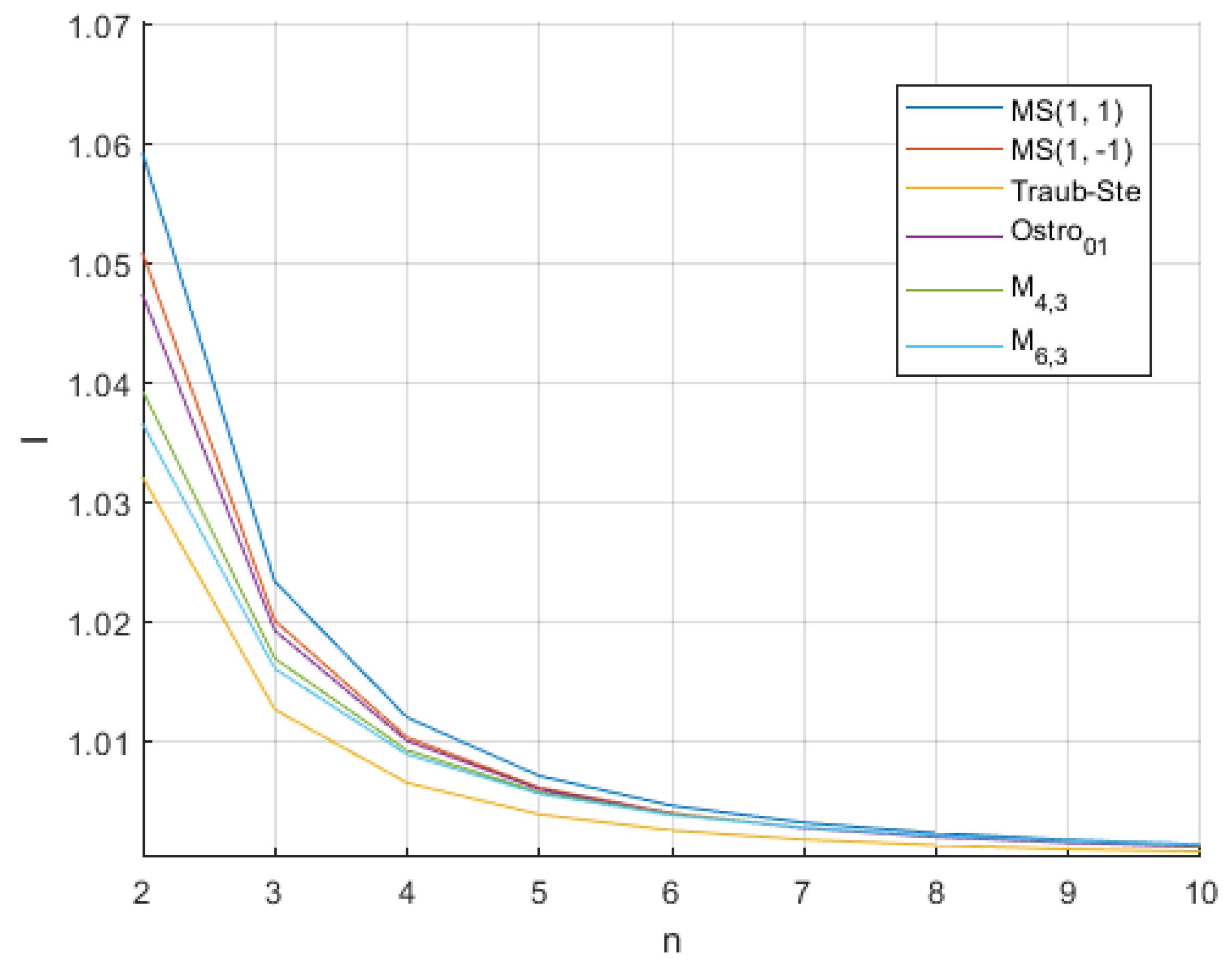
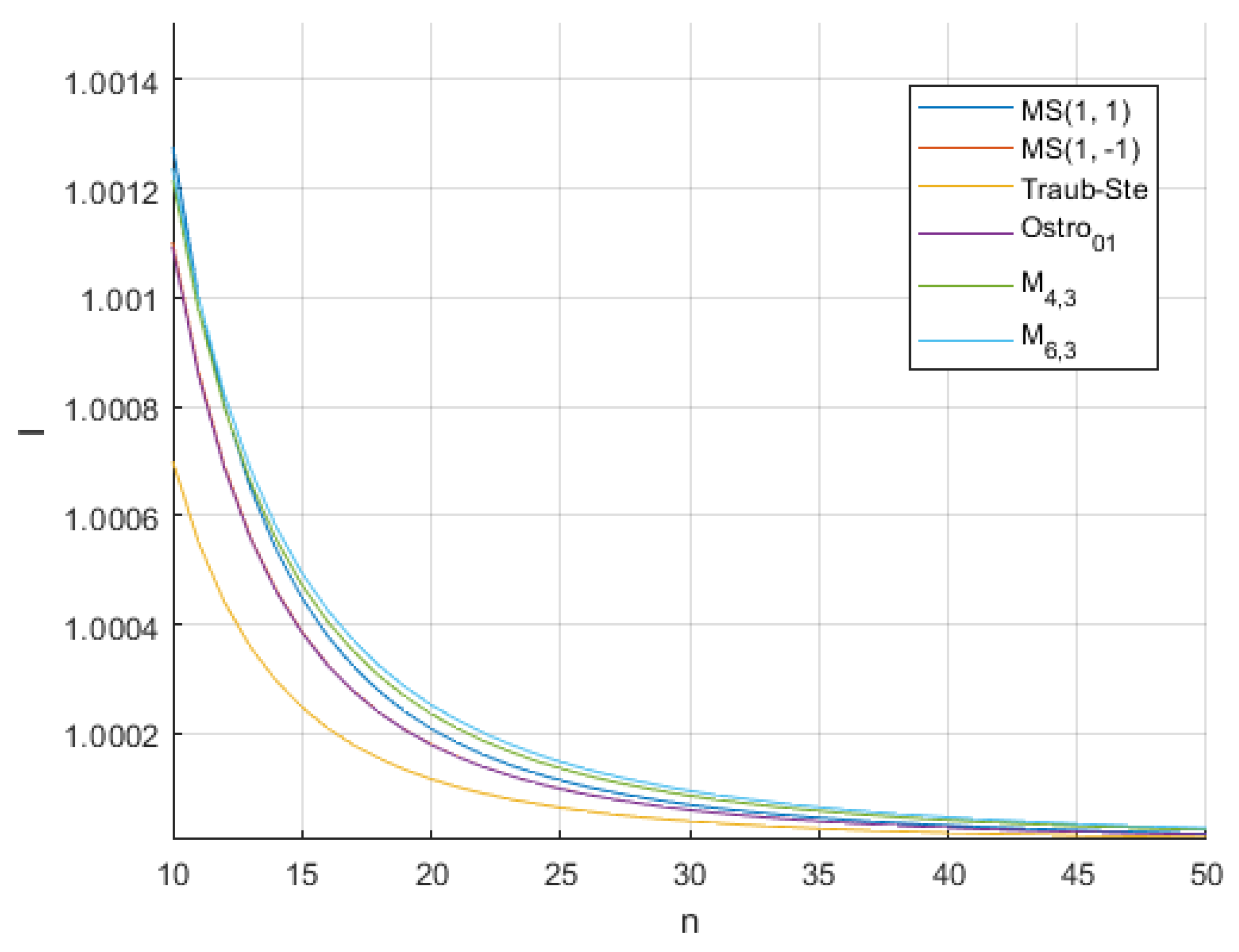
In order to show more clearly how computational cost influences the efficiency index $I=p^{{\displaystyle \frac{1}{C}}}$, where p is the convergence order of the corresponding scheme (see [24]), we present Figure 1 and Figure 2 for different sizes of the nonlinear system to be solved.

Figure 1. I indices for $MS(p_1,p_2)$ and comparison methods.

Figure 2. I indices for $MS(p_1,p_2)$ and comparison schemes.

In Figure 1, we observe that for systems with dimensions $n=2,3,\dots ,10$, the proposed class of vectorial iterative methods (9) shows better computational efficiency than the other schemes, for both members of the family. On the other hand, as the system grows to sizes $n=10,11,\dots ,50$, it becomes apparent that methods $M_{4,3}$ and $M_{6,3}$ yield better results. Let us notice that for sizes of $n<11$, our method has better efficiency than $M_{6,3}$, and for sizes $n<12$, it has better efficiency compared to $M_{4,3}$ (see Figure 2).

In the next section, we check the theoretical convergence order of our proposed method and assess the efficiency of different schemes in nonlinear systems of various sizes.

4. Numerical Results

In this section, we test numerically whether or not the theoretical order holds for practical purposes in the proposed Jacobian-free class (9). Moreover, we compare it with the methods that appeared in the efficiency section to show their accuracy and computational performance.

Numerical results were obtained with the Matlab2022b version, using 8000 digits in variable precision arithmetics, a processor AMD A12-9720P RADEON R7, 12 COMPUTE CORES 4C, +8G-Ram, and 2.70 GHz. The results are shown in Table 2, Table 3, Table 4, Table 5, Table 6, Table 7, Table 8, Table 9, Table 10, Table 11, Table 12 and Table 13, including the following information, where the appearing norms are Euclidean:

• k: amount of iterations needed (“-” appears when the scheme does not converge or it needs more iterations than the maximum allowed).
• $\overline{\xi }$: obtained solution.
• Cpu-time: average time in seconds required by the iterative method to reach the solution of the problem when executed ten times.
• $\rho$: approximated computational order of convergence, ACOC, firstly appearing in [25]

  $$\rho ={\displaystyle \frac{ln\frac{∥x^{(k+1)}-x^{\left(k\right)}∥}{∥x^{\left(k\right)}-x^{(k-1)}∥}}{ln\frac{∥x^{\left(k\right)}-x^{(k-1)}∥}{∥x^{(k-1)}-x^{(k-2)}∥}}},k=2,3,\dots ,$$
  (if $\rho$ is not stable, then “-” appears in the table).
• ${ϵ}_{aprox}=∥x^{(k+1)}-x^{\left(k\right)}∥$.
• ${ϵ}_f=∥F\left(x^{(k+1)}\right)∥$. If ${ϵ}_f$ or ${ϵ}_{aprox}$ are very far from zero or we reach infinity or NAN, then “-” appears in the table.

Regarding the stopping criterium, the iterative process ends when one of the following conditions is fulfilled:

(i)

$∥F\left(x^{(k+1)}\right)∥<{10}^{-100}$;

(ii)

$∥x^{(k+1)}-x^{\left(k\right)}∥<{10}^{-100}$;

(iii)

Fifty iterations are reached.

4.1. Academic Problems

We include a wide variety of nonlinear systems with different dimensions, ranging from 2 to 25. The diversity of expressions present in these systems ensures the versatility of the methods applied and their efficiency.

Example 1.

The first case we present is a system $F^1\left(x\right)={\left(f_1^1\left(x\right),f_2^1\left(x\right),\dots ,f_{25}^1\left(x\right)\right)}^T$, where

$$\begin{array}{c}\hfill \left\{\begin{array}{cc}{f}_i^1\left(x\right)\hfill & =x_i^2{x}_{i+1}-1,i=1,2,\dots ,24,\hfill \\ f_{25}^1\left(x\right)\hfill & =x_{25}^2{x}_1-1.\hfill \end{array}\right.\end{array}$$

the solution for which is $\overline{\xi }=(1,1,1,\dots ,1)$.

Table 2. Results for function $F^1$, using as a seed $x^{\left(0\right)}=(1.5,1.5,1.5,\dots ,1.5)$.

Iterative Method	k	$\mathit{\rho }$	${\mathit{ϵ}}_{\mathit{aprox}}$	${\mathit{ϵ}}_{\mathit{f}}$	$\overline{\mathit{\xi }}$	Cpu-Time
$MS(1,-1)$	7	4.00	1.108 × ${10}^{-51}$	4.624 × ${10}^{-204}$	${\overline{\xi }}_1$	191.7242
$MS(1,1)$	5	4.97	4.904 × ${10}^{-24}$	3.995 × ${10}^{-117}$	${\overline{\xi }}_1$	143.1027
Traub-Ste	5	4.00	1.241 × ${10}^{-35}$	1.517 × ${10}^{-140}$	${\overline{\xi }}_1$	227.8747
$Ostr{o}_{01}$	-	-	-	-	-	-
$M_{4,3}$	6	4.00	7.338 × ${10}^{-40}$	3.015 × ${10}^{-158}$	${\overline{\xi }}_1$	163.9808
$M_{6,3}$	5	5.96	1.336 × ${10}^{-47}$	7.876 × ${10}^{-284}$	${\overline{\xi }}_1$	142.6446

Table 2. Results for function $F^1$, using as a seed $x^{\left(0\right)}=(1.5,1.5,1.5,\dots ,1.5)$.

Iterative Method	k	$\mathit{\rho }$	${\mathit{ϵ}}_{\mathit{aprox}}$	${\mathit{ϵ}}_{\mathit{f}}$	$\overline{\mathit{\xi }}$	Cpu-Time
$MS(1,-1)$	7	4.00	1.108 × ${10}^{-51}$	4.624 × ${10}^{-204}$	${\overline{\xi }}_1$	191.7242
$MS(1,1)$	5	4.97	4.904 × ${10}^{-24}$	3.995 × ${10}^{-117}$	${\overline{\xi }}_1$	143.1027
Traub-Ste	5	4.00	1.241 × ${10}^{-35}$	1.517 × ${10}^{-140}$	${\overline{\xi }}_1$	227.8747
$Ostr{o}_{01}$	-	-	-	-	-	-
$M_{4,3}$	6	4.00	7.338 × ${10}^{-40}$	3.015 × ${10}^{-158}$	${\overline{\xi }}_1$	163.9808
$M_{6,3}$	5	5.96	1.336 × ${10}^{-47}$	7.876 × ${10}^{-284}$	${\overline{\xi }}_1$	142.6446

In Table 2, the $Ostr{o}_{01}$ method reached the maximum number of iterations without converging to the solution, while the most notable scheme is $M_{6,3}$ in almost all aspects, such as errors, iterations and computational time. On the other hand, although $MS(1,1)$ exhibits a lower computational time than $M_{4,3}$, the latter has an additional iteration, a relatively similar time, and better errors, proving that it might even be superior in terms of efficiency.

Example 2.

The second case we present is a system $F^2\left(x\right)={\left(f_1^2\left(x\right),f_2^2\left(x\right),\dots ,f_8^2\left(x\right)\right)}^T$, where

$$f_i^2\left(x\right)=x_i-cos\left(2x_i-\sum _{k=1}^8{x}_k\right),i=1,2,\dots ,8,$$

$\overline{\xi }\approx (0.5149,0.5149,\dots ,0.5149)$ being its solution.

Table 3. Numerical results for $F^2$, $x^{\left(0\right)}=(1,1,1,\dots ,1)$.

Iterative Method	k	$\mathit{\rho }$	${\mathit{ϵ}}_{\mathit{aprox}}$	${\mathit{ϵ}}_{\mathit{f}}$	$\overline{\mathit{\xi }}$	Cpu-Time
$MS(1,-1)$	8	3.99	2.794 × ${10}^{-29}$	4.092 × ${10}^{-115}$	${\overline{\xi }}_1$	73.3126
$MS(1,1)$	8	5.00	7.534 × ${10}^{-74}$	2.162 × ${10}^{-366}$	${\overline{\xi }}_1$	72.6143
Traub-Ste	16	4.00	9.389 × ${10}^{-68}$	3.459 × ${10}^{-269}$	${\overline{\xi }}_1$	317.9304
$Ostr{o}_{01}$	15	4.00	6.341 × ${10}^{-70}$	1.641 × ${10}^{-278}$	${\overline{\xi }}_1$	139.3808
$M_{4,3}$	7	4.00	8.510 × ${10}^{-87}$	3.949 × ${10}^{-346}$	${\overline{\xi }}_1$	76.9114
$M_{6,3}$	6	6.02	4.223 × ${10}^{-47}$	8.063 × ${10}^{-281}$	${\overline{\xi }}_1$	79.7898

Table 3. Numerical results for $F^2$, $x^{\left(0\right)}=(1,1,1,\dots ,1)$.

Iterative Method	k	$\mathit{\rho }$	${\mathit{ϵ}}_{\mathit{aprox}}$	${\mathit{ϵ}}_{\mathit{f}}$	$\overline{\mathit{\xi }}$	Cpu-Time
$MS(1,-1)$	8	3.99	2.794 × ${10}^{-29}$	4.092 × ${10}^{-115}$	${\overline{\xi }}_1$	73.3126
$MS(1,1)$	8	5.00	7.534 × ${10}^{-74}$	2.162 × ${10}^{-366}$	${\overline{\xi }}_1$	72.6143
Traub-Ste	16	4.00	9.389 × ${10}^{-68}$	3.459 × ${10}^{-269}$	${\overline{\xi }}_1$	317.9304
$Ostr{o}_{01}$	15	4.00	6.341 × ${10}^{-70}$	1.641 × ${10}^{-278}$	${\overline{\xi }}_1$	139.3808
$M_{4,3}$	7	4.00	8.510 × ${10}^{-87}$	3.949 × ${10}^{-346}$	${\overline{\xi }}_1$	76.9114
$M_{6,3}$	6	6.02	4.223 × ${10}^{-47}$	8.063 × ${10}^{-281}$	${\overline{\xi }}_1$	79.7898

In Table 3, we observe that our proposed schemes yield the best computational times, with the $MS(1,1)$ method standing out for having the smallest error norm among all schemes. The $M_{4,3}$ method, while showing good overall performance in terms of errors, is more computationally expensive as it takes one iteration longer to reach the solution to the system and slightly more time compared to $MS(p1,p2)$ methods, indicating that the program takes more time to generate each iteration.

Example 3.

The third case we present is a system $F^3\left(x\right)={\left(f_1^3\left(x\right),f_2^3\left(x\right),\dots ,f_5^3\left(x\right)\right)}^T$, where

$$f_i^3\left(x\right)=\sum _{k=1}^5\left(x_k\right)-x_i-e^{(-x_i)},i=1,2,3,4,5,$$

where the solution is $\overline{\xi }\approx (0.20389,0.20389,0.20389,\dots ,0.20389)$.

The corresponding numerical results appear in Table 4, where the $MS(1,1)$ method shows the best errors, while the shortest computational time is achieved by the $M_{6,3}$ method.

Table 4. Numerical results for $F^3$, $x^{\left(0\right)}=(0.5,0.5,0.5,0.5,0.5)$.

Iterative Method	k	$\mathit{\rho }$	${\mathit{ϵ}}_{\mathit{aprox}}$	${\mathit{ϵ}}_{\mathit{f}}$	$\overline{\mathit{\xi }}$	Cpu-Time
$MS(1,-1)$	4	4.00	1.305 × ${10}^{-55}$	2.980 × ${10}^{-221}$	${\overline{\xi }}_1$	12.8166
$MS(1,1)$	4	5.00	4.997 × ${10}^{-101}$	1.143 × ${10}^{-503}$	${\overline{\xi }}_1$	12.6105
Traub-Ste	4	4.00	9.461 × ${10}^{-68}$	1.372 × ${10}^{-270}$	${\overline{\xi }}_1$	18.9457
$Ostr{o}_{01}$	4	4.00	1.420 × ${10}^{-47}$	2.882 × ${10}^{-189}$	${\overline{\xi }}_1$	12.4768
$M_{4,3}$	4	4.00	3.440 × ${10}^{-44}$	1.007 × ${10}^{-175}$	${\overline{\xi }}_1$	12.8707
$M_{6,3}$	3	6.07	1.482 × ${10}^{-21}$	3.012 × ${10}^{-127}$	${\overline{\xi }}_1$	10.5536

Table 4. Numerical results for $F^3$, $x^{\left(0\right)}=(0.5,0.5,0.5,0.5,0.5)$.

Iterative Method	k	$\mathit{\rho }$	${\mathit{ϵ}}_{\mathit{aprox}}$	${\mathit{ϵ}}_{\mathit{f}}$	$\overline{\mathit{\xi }}$	Cpu-Time
$MS(1,-1)$	4	4.00	1.305 × ${10}^{-55}$	2.980 × ${10}^{-221}$	${\overline{\xi }}_1$	12.8166
$MS(1,1)$	4	5.00	4.997 × ${10}^{-101}$	1.143 × ${10}^{-503}$	${\overline{\xi }}_1$	12.6105
Traub-Ste	4	4.00	9.461 × ${10}^{-68}$	1.372 × ${10}^{-270}$	${\overline{\xi }}_1$	18.9457
$Ostr{o}_{01}$	4	4.00	1.420 × ${10}^{-47}$	2.882 × ${10}^{-189}$	${\overline{\xi }}_1$	12.4768
$M_{4,3}$	4	4.00	3.440 × ${10}^{-44}$	1.007 × ${10}^{-175}$	${\overline{\xi }}_1$	12.8707
$M_{6,3}$	3	6.07	1.482 × ${10}^{-21}$	3.012 × ${10}^{-127}$	${\overline{\xi }}_1$	10.5536

Example 4.

The fourth case we present is a system $F^4\left(x\right)={\left(f_1^4\left(x\right),f_2^4\left(x\right),\dots ,f_5^4\left(x\right)\right)}^T$, where

$$f_i^4\left(x\right)=\sum _{k=1}^5\left(x_k\right)-x_i-e^{(-x_i)}{x}_i,i=1,2,3,4,5,$$

the solution for which $\overline{\xi }=(0,0,0,\dots ,0)$.

Table 5. Numerical results for $F^4$, $x^{\left(0\right)}=(0.5,0.5,0.5,0.5,0.5)$.

Iterative Method	k	$\mathit{\rho }$	${\mathit{ϵ}}_{\mathit{aprox}}$	${\mathit{ϵ}}_{\mathit{f}}$	$\overline{\mathit{\xi }}$	Cpu-Time
$MS(1,-1)$	4	3.99	7.838 × ${10}^{-31}$	4.801 × ${10}^{-121}$	${\overline{\xi }}_1$	14.6365
$MS(1,1)$	4	5.00	2.864 × ${10}^{-52}$	2.514 × ${10}^{-258}$	${\overline{\xi }}_1$	14.6532
Traub-Ste	4	4.00	8.656 × ${10}^{-34}$	3.124 × ${10}^{-133}$	${\overline{\xi }}_1$	21.7138
$Ostr{o}_{01}$	4	4.00	2.268 × ${10}^{-35}$	6.443 × ${10}^{-140}$	${\overline{\xi }}_1$	14.0140
$M_{4,3}$	4	4.00	2.594 × ${10}^{-47}$	9.227 × ${10}^{-188}$	${\overline{\xi }}_1$	14.8093
$M_{6,3}$	3	5.32	6.593 × ${10}^{-26}$	7.254 × ${10}^{-153}$	${\overline{\xi }}_1$	12.0667

Table 5. Numerical results for $F^4$, $x^{\left(0\right)}=(0.5,0.5,0.5,0.5,0.5)$.

Iterative Method	k	$\mathit{\rho }$	${\mathit{ϵ}}_{\mathit{aprox}}$	${\mathit{ϵ}}_{\mathit{f}}$	$\overline{\mathit{\xi }}$	Cpu-Time
$MS(1,-1)$	4	3.99	7.838 × ${10}^{-31}$	4.801 × ${10}^{-121}$	${\overline{\xi }}_1$	14.6365
$MS(1,1)$	4	5.00	2.864 × ${10}^{-52}$	2.514 × ${10}^{-258}$	${\overline{\xi }}_1$	14.6532
Traub-Ste	4	4.00	8.656 × ${10}^{-34}$	3.124 × ${10}^{-133}$	${\overline{\xi }}_1$	21.7138
$Ostr{o}_{01}$	4	4.00	2.268 × ${10}^{-35}$	6.443 × ${10}^{-140}$	${\overline{\xi }}_1$	14.0140
$M_{4,3}$	4	4.00	2.594 × ${10}^{-47}$	9.227 × ${10}^{-188}$	${\overline{\xi }}_1$	14.8093
$M_{6,3}$	3	5.32	6.593 × ${10}^{-26}$	7.254 × ${10}^{-153}$	${\overline{\xi }}_1$	12.0667

The results in Table 5 are similar to those in Table 4. They are very balanced, with the $MS(1,1)$ method presenting the best errors, while the shortest computational time is achieved by the $M_{6,3}$ method. However, this last one requires more effort to generate an iteration because, despite it producing one less iteration than the other iterative methods, their execution times are very similar.

Example 5.

The fifth case we present is a system $F^5\left(x\right)={\left(f_1^5\left(x\right),f_2^5\left(x\right),\dots ,f_{10}^5\left(x\right)\right)}^T$, where

$$f_i^5\left(x\right)=x_i+1-2log\left(1-x_i+\sum _{k=1}^{10}\left(x_k\right)\right),i=1,2,3,\dots ,10,$$

its solution being $\overline{\xi }\approx (7.4370,7.4370,\dots ,7.4370)$.

Table 6. Numerical results for $F^5$, $x^{\left(0\right)}=(7,7,7,\dots ,7)$.

Iterative Method	k	$\mathit{\rho }$	${\mathit{ϵ}}_{\mathit{aprox}}$	${\mathit{ϵ}}_{\mathit{f}}$	$\overline{\mathit{\xi }}$	Cpu-Time
$MS(1,-1)$	3	4.03	1.343 × ${10}^{-24}$	1.076 × ${10}^{-101}$	${\overline{\xi }}_1$	58.6649
$MS(1,1)$	3	5.03	5.715 × ${10}^{-36}$	1.098 × ${10}^{-183}$	${\overline{\xi }}_1$	58.6010
Traub-Ste	4	4.00	2.252 × ${10}^{-97}$	1.397 × ${10}^{-392}$	${\overline{\xi }}_1$	138.3238
$Ostr{o}_{01}$	4	4.00	1.317 × ${10}^{-99}$	1.705 × ${10}^{-401}$	${\overline{\xi }}_1$	76.6871
$M_{4,3}$	3	4.00	1.490 × ${10}^{-24}$	2.175 × ${10}^{-101}$	${\overline{\xi }}_1$	64.3101
$M_{6,3}$	3	6.01	1.565 × ${10}^{-53}$	4.782 × ${10}^{-326}$	${\overline{\xi }}_1$	69.4223

Table 6. Numerical results for $F^5$, $x^{\left(0\right)}=(7,7,7,\dots ,7)$.

Iterative Method	k	$\mathit{\rho }$	${\mathit{ϵ}}_{\mathit{aprox}}$	${\mathit{ϵ}}_{\mathit{f}}$	$\overline{\mathit{\xi }}$	Cpu-Time
$MS(1,-1)$	3	4.03	1.343 × ${10}^{-24}$	1.076 × ${10}^{-101}$	${\overline{\xi }}_1$	58.6649
$MS(1,1)$	3	5.03	5.715 × ${10}^{-36}$	1.098 × ${10}^{-183}$	${\overline{\xi }}_1$	58.6010
Traub-Ste	4	4.00	2.252 × ${10}^{-97}$	1.397 × ${10}^{-392}$	${\overline{\xi }}_1$	138.3238
$Ostr{o}_{01}$	4	4.00	1.317 × ${10}^{-99}$	1.705 × ${10}^{-401}$	${\overline{\xi }}_1$	76.6871
$M_{4,3}$	3	4.00	1.490 × ${10}^{-24}$	2.175 × ${10}^{-101}$	${\overline{\xi }}_1$	64.3101
$M_{6,3}$	3	6.01	1.565 × ${10}^{-53}$	4.782 × ${10}^{-326}$	${\overline{\xi }}_1$	69.4223

For Table 6, we note that the best computational times are obtained by the methods $MS(p1,p2)$. On the other hand, the best errors are obtained by the $Ostr{o}_{01}$ scheme, which has a competitive computational time considering it requires four iterations, similar to Traub-Ste. The latter has been shown to be the one that requires the most time to converge.

Example 6.

The sixth case we present is a system $F^6\left(x\right)={\left(f_1^6\left(x\right),f_2^6\left(x\right),\dots ,f_5^6\left(x\right)\right)}^T$, where

$$f_i^6\left(x\right)=x_i+1.5sin\left(\sum _{k=1}^5\left(x_k\right)-x_i\right),i=1,2,3,4,5,$$

and there exist two solutions, ${\overline{\xi }}_1\approx (-0.3004,-0.3004,\dots ,-0.3004)$ and ${\overline{\xi }}_2\approx (0.4579,0.4579,\dots ,0.4579)$.

Table 7. Numerical results for $F^6$$x^{\left(0\right)}=(0.75,0.75,0.75,0.75,0.75)$.

Iterative Method	k	$\mathit{\rho }$	${\mathit{ϵ}}_{\mathit{aprox}}$	${\mathit{ϵ}}_{\mathit{f}}$	$\overline{\mathit{\xi }}$	Cpu-Time
$MS(1,-1)$	6	4.00	5.425 × ${10}^{-88}$	5.270 × ${10}^{-349}$	${\overline{\xi }}_1$	20.2517
$MS(1,1)$	5	4.97	5.922 × ${10}^{-39}$	1.965 × ${10}^{-190}$	${\overline{\xi }}_1$	16.9191
Traub-Ste	20	4.00	9.536 × ${10}^{-99}$	4.618 × ${10}^{-391}$	${\overline{\xi }}_2$	154.5691
$Ostr{o}_{01}$	5	4.00	1.050 × ${10}^{-33}$	2.164 × ${10}^{-132}$	${\overline{\xi }}_1$	16.5869
$M_{4,3}$	10	4.01	3.127 × ${10}^{-35}$	1.500 × ${10}^{-138}$	${\overline{\xi }}_1$	51.2143
$M_{6,3}$	17	5.90	6.480 × ${10}^{-23}$	2.076 × ${10}^{-132}$	${\overline{\xi }}_2$	105.4212

Table 7. Numerical results for $F^6$$x^{\left(0\right)}=(0.75,0.75,0.75,0.75,0.75)$.

Iterative Method	k	$\mathit{\rho }$	${\mathit{ϵ}}_{\mathit{aprox}}$	${\mathit{ϵ}}_{\mathit{f}}$	$\overline{\mathit{\xi }}$	Cpu-Time
$MS(1,-1)$	6	4.00	5.425 × ${10}^{-88}$	5.270 × ${10}^{-349}$	${\overline{\xi }}_1$	20.2517
$MS(1,1)$	5	4.97	5.922 × ${10}^{-39}$	1.965 × ${10}^{-190}$	${\overline{\xi }}_1$	16.9191
Traub-Ste	20	4.00	9.536 × ${10}^{-99}$	4.618 × ${10}^{-391}$	${\overline{\xi }}_2$	154.5691
$Ostr{o}_{01}$	5	4.00	1.050 × ${10}^{-33}$	2.164 × ${10}^{-132}$	${\overline{\xi }}_1$	16.5869
$M_{4,3}$	10	4.01	3.127 × ${10}^{-35}$	1.500 × ${10}^{-138}$	${\overline{\xi }}_1$	51.2143
$M_{6,3}$	17	5.90	6.480 × ${10}^{-23}$	2.076 × ${10}^{-132}$	${\overline{\xi }}_2$	105.4212

In Table 7, the best errors were obtained by $MS(1,-1)$ and Traub-Ste, which converged to different solutions, while in terms of performance, $MS(1,1)$ and $Ostr{o}_{01}$ appeared to be better.

Example 7.

The seventh case we present is a system $F^7\left(x\right)={\left(f_1^7\left(x\right),f_2^7\left(x\right)\right)}^T$, where

$$F_i^7\left(x\right)=arctan\left(x_i\right)+1-2\left[\left({\displaystyle \sum _{k=1}^2{x}_k^2}\right)-x_i^2\right]=0,\mathrm{i}=1,2,$$

and $\overline{\xi }\approx (0.936,0.936)$.

Table 8. Numerical results for $F^7$, $x^{\left(0\right)}=(0.25,0.25)$.

Iterative Method	k	$\mathit{\rho }$	${\mathit{ϵ}}_{\mathit{aprox}}$	${\mathit{ϵ}}_{\mathit{f}}$	$\overline{\mathit{\xi }}$	Cpu-Time
$MS(1,-1)$	5	4.00	5.203 × ${10}^{-41}$	6.322 × ${10}^{-161}$	${\overline{\xi }}_1$	3.6588
$MS(1,1)$	4	5.00	5.282 × ${10}^{-73}$	6.419 × ${10}^{-362}$	${\overline{\xi }}_1$	3.0030
Traub-Ste	6	4.00	6.615 × ${10}^{-81}$	7.658 × ${10}^{-321}$	${\overline{\xi }}_1$	4.6891
$Ostr{o}_{01}$	-	-	-	-	-	-
$M_{4,3}$	6	4.00	5.613 × ${10}^{-98}$	3.787 × ${10}^{-389}$	${\overline{\xi }}_1$	3.7011
$M_{6,3}$	7	5.92	2.032 × ${10}^{-32}$	5.723 × ${10}^{-190}$	${\overline{\xi }}_1$	4.4699

Table 8. Numerical results for $F^7$, $x^{\left(0\right)}=(0.25,0.25)$.

Iterative Method	k	$\mathit{\rho }$	${\mathit{ϵ}}_{\mathit{aprox}}$	${\mathit{ϵ}}_{\mathit{f}}$	$\overline{\mathit{\xi }}$	Cpu-Time
$MS(1,-1)$	5	4.00	5.203 × ${10}^{-41}$	6.322 × ${10}^{-161}$	${\overline{\xi }}_1$	3.6588
$MS(1,1)$	4	5.00	5.282 × ${10}^{-73}$	6.419 × ${10}^{-362}$	${\overline{\xi }}_1$	3.0030
Traub-Ste	6	4.00	6.615 × ${10}^{-81}$	7.658 × ${10}^{-321}$	${\overline{\xi }}_1$	4.6891
$Ostr{o}_{01}$	-	-	-	-	-	-
$M_{4,3}$	6	4.00	5.613 × ${10}^{-98}$	3.787 × ${10}^{-389}$	${\overline{\xi }}_1$	3.7011
$M_{6,3}$	7	5.92	2.032 × ${10}^{-32}$	5.723 × ${10}^{-190}$	${\overline{\xi }}_1$	4.4699

In Table 8, the $Ostr{o}_{01}$ method could not converge to the solution because it reached the maximum number of iterations, whereas the $MS(p1,p2)$ and $M_{4,3}$ methods showed better overall behavior.

4.2. Special Problems

In the following cases, we address problems of interest where we demonstrate the advantages of our method applied to three types of systems: a non-differentiable system, a high-dimensional system, and a system with real-world applications.

We present a non-differentiable system of size $n\times n$ with $n=2$, which includes both transcendental and algebraic functions, such as the absolute value. These characteristics justify the use of derivative-free numerical schemes, as proposed in this work, to obtain the desired results. To demonstrate the effectiveness and robustness of our method, we will solve the problem using five different initial estimates, thereby showcasing its general good performance when addressing such problems.

Example 8.

The eighth case we present is a system $F^8\left(x\right)={\left(f_1^8\left(x\right),f_2^8\left(x\right)\right)}^T$, where

$$\begin{array}{cc}\hfill f_1^8\left(x\right)& =log\left(\right|x_1\left|\right)+|x_2|,\hfill \\ \hfill f_2^8\left(x\right)& =e^{\left(x_1\right)}+x_2-1,\hfill \end{array}$$

with solutions ${\overline{\xi }}_1\approx (-0.6275,0.4661)$ and ${\overline{\xi }}_2\approx (0.5122,-0.669)$.

Table 9. Numerical results for $F^8$, $x^{\left(0\right)}=(0.25,0.25)$.

Iterative Method	k	$\mathit{\rho }$	${\mathit{ϵ}}_{\mathit{aprox}}$	${\mathit{ϵ}}_{\mathit{f}}$	$\overline{\mathit{\xi }}$	Cpu-Time
$MS(1,-1)$	4	4.00	1.139 × ${10}^{-54}$	9.420 × ${10}^{-217}$	${\overline{\xi }}_1$	2.9146
$MS(1,1)$	4	4.20	1.415 × ${10}^{-72}$	2.272 × ${10}^{-301}$	${\overline{\xi }}_1$	2.8907
Traub-Ste	4	4.11	4.417 × ${10}^{-48}$	1.391 × ${10}^{-191}$	${\overline{\xi }}_1$	3.1954
$Ostr{o}_{01}$	6	4.00	2.520 × ${10}^{-78}$	1.241 × ${10}^{-310}$	${\overline{\xi }}_1$	3.4855
$M_{4,3}$	7	4.02	1.401 × ${10}^{-72}$	3.093 × ${10}^{-288}$	${\overline{\xi }}_1$	4.0501
$M_{6,3}$	6	6.27	4.634 × ${10}^{-58}$	7.902 × ${10}^{-346}$	${\overline{\xi }}_1$	3.6475

Table 9. Numerical results for $F^8$, $x^{\left(0\right)}=(0.25,0.25)$.

Iterative Method	k	$\mathit{\rho }$	${\mathit{ϵ}}_{\mathit{aprox}}$	${\mathit{ϵ}}_{\mathit{f}}$	$\overline{\mathit{\xi }}$	Cpu-Time
$MS(1,-1)$	4	4.00	1.139 × ${10}^{-54}$	9.420 × ${10}^{-217}$	${\overline{\xi }}_1$	2.9146
$MS(1,1)$	4	4.20	1.415 × ${10}^{-72}$	2.272 × ${10}^{-301}$	${\overline{\xi }}_1$	2.8907
Traub-Ste	4	4.11	4.417 × ${10}^{-48}$	1.391 × ${10}^{-191}$	${\overline{\xi }}_1$	3.1954
$Ostr{o}_{01}$	6	4.00	2.520 × ${10}^{-78}$	1.241 × ${10}^{-310}$	${\overline{\xi }}_1$	3.4855
$M_{4,3}$	7	4.02	1.401 × ${10}^{-72}$	3.093 × ${10}^{-288}$	${\overline{\xi }}_1$	4.0501
$M_{6,3}$	6	6.27	4.634 × ${10}^{-58}$	7.902 × ${10}^{-346}$	${\overline{\xi }}_1$	3.6475

In Table 9, the $MS(1,1)$ method stands out with the lowest computational time, being more efficient than the others, despite requiring a similar number of iterations and showing a convergence order of $4.20$, which is close to that of the other methods. The Traub-Ste method is less efficient, with a computational time of $3.1954$ but with a larger errors. $Ostr{o}_{01}$ is competitive, only falling slightly behind in computational time. Methods $M_{4,3}$ and $M_{6,3}$ are the most expensive in terms of computational time, requiring seven and six iterations, respectively, with the highest time recorded for $M_{4,3}$. Despite their higher orders of convergence, both methods show lower overall efficiency compared to the $MS$ and $Ostro01$ methods.

Table 10. Numerical results for $F^8$, $x^{\left(0\right)}=(1.25,1.25)$.

Iterative Method	k	$\mathit{\rho }$	${\mathit{ϵ}}_{\mathit{aprox}}$	${\mathit{ϵ}}_{\mathit{f}}$	$\overline{\mathit{\xi }}$	Cpu-Time
$MS(1,-1)$	6	4.00	1.019 × ${10}^{-65}$	6.029 × ${10}^{-261}$	${\overline{\xi }}_1$	4.1403
$MS(1,1)$	5	4.05	2.474 × ${10}^{-42}$	4.929 × ${10}^{-177}$	${\overline{\xi }}_1$	3.3999
Traub-Ste	6	4.00	8.946 × ${10}^{-86}$	2.341 × ${10}^{-342}$	${\overline{\xi }}_1$	4.4433
$Ostr{o}_{01}$	8	4.00	2.050 × ${10}^{-55}$	5.429 × ${10}^{-219}$	${\overline{\xi }}_1$	4.4246
$M_{4,3}$	-	-	-	-	-	-
$M_{6,3}$	-	-	-	-	-	-

Table 10. Numerical results for $F^8$, $x^{\left(0\right)}=(1.25,1.25)$.

Iterative Method	k	$\mathit{\rho }$	${\mathit{ϵ}}_{\mathit{aprox}}$	${\mathit{ϵ}}_{\mathit{f}}$	$\overline{\mathit{\xi }}$	Cpu-Time
$MS(1,-1)$	6	4.00	1.019 × ${10}^{-65}$	6.029 × ${10}^{-261}$	${\overline{\xi }}_1$	4.1403
$MS(1,1)$	5	4.05	2.474 × ${10}^{-42}$	4.929 × ${10}^{-177}$	${\overline{\xi }}_1$	3.3999
Traub-Ste	6	4.00	8.946 × ${10}^{-86}$	2.341 × ${10}^{-342}$	${\overline{\xi }}_1$	4.4433
$Ostr{o}_{01}$	8	4.00	2.050 × ${10}^{-55}$	5.429 × ${10}^{-219}$	${\overline{\xi }}_1$	4.4246
$M_{4,3}$	-	-	-	-	-	-
$M_{6,3}$	-	-	-	-	-	-

In Table 10, method $MS(1,1)$ stands out as the one with the lowest computational time, requiring fewer iterations compared to the other methods and showing a convergence order of 4.05. The Traub-Ste method, despite having the same convergence order as $MS(1,-1)$, shows a slightly higher computational time and larger errors in the difference between iterates. $Ostr{o}_{01}$, which requires more iterations, falls only slightly behind in computational time but remains competitive overall. Methods $M_{4,3}$ and $M_{6,3}$ do not converge to the solution, as division by zero occurred when calculating the divided differences.

Table 11. Numerical results for $F^8$, $x^{\left(0\right)}=(2,2)$.

Iterative Method	k	$\mathit{\rho }$	${\mathit{ϵ}}_{\mathit{aprox}}$	${\mathit{ϵ}}_{\mathit{f}}$	$\overline{\mathit{\xi }}$	Cpu-Time
$MS(1,-1)$	10	4.00	6.679 × ${10}^{-71}$	1.113 × ${10}^{-281}$	${\overline{\xi }}_1$	6.9568
$MS(1,1)$	8	4.28	4.387 × ${10}^{-77}$	3.113 × ${10}^{-321}$	${\overline{\xi }}_1$	5.4126
Traub-Ste	15	4.00	4.978 × ${10}^{-100}$	2.442 × ${10}^{-397}$	${\overline{\xi }}_2$	10.6624
$Ostr{o}_{01}$	-	-	-	-	-	-
$M_{4,3}$	-	-	-	-	-	-
$M_{6,3}$	-	-	-	-	-	-

Table 11. Numerical results for $F^8$, $x^{\left(0\right)}=(2,2)$.

Iterative Method	k	$\mathit{\rho }$	${\mathit{ϵ}}_{\mathit{aprox}}$	${\mathit{ϵ}}_{\mathit{f}}$	$\overline{\mathit{\xi }}$	Cpu-Time
$MS(1,-1)$	10	4.00	6.679 × ${10}^{-71}$	1.113 × ${10}^{-281}$	${\overline{\xi }}_1$	6.9568
$MS(1,1)$	8	4.28	4.387 × ${10}^{-77}$	3.113 × ${10}^{-321}$	${\overline{\xi }}_1$	5.4126
Traub-Ste	15	4.00	4.978 × ${10}^{-100}$	2.442 × ${10}^{-397}$	${\overline{\xi }}_2$	10.6624
$Ostr{o}_{01}$	-	-	-	-	-	-
$M_{4,3}$	-	-	-	-	-	-
$M_{6,3}$	-	-	-	-	-	-

Method $MS(1,1)$ stands out as the one with the lowest computational time, requiring fewer iterations compared to the other methods and showing a convergence order of $4.28$. The Traub-Ste scheme, despite having the same convergence order as $MS(1,-1)$, shows a significantly higher computational time but better results in terms of errors. $MS(1,-1)$, while requiring more iterations than $MS(1,1)$, still maintains a competitive time compared to Traub-Ste. Division by zero is the reason why the other methods could not reach the solution.

Table 12. Numerical results for $F^8$, $x^{\left(0\right)}=(2.25,2.25)$.

Iterative Method	k	$\mathit{\rho }$	${\mathit{ϵ}}_{\mathit{aprox}}$	${\mathit{ϵ}}_{\mathit{f}}$	$\overline{\mathit{\xi }}$	Cpu-Time
$MS(1,-1)$	16	4.00	2.821 × ${10}^{-94}$	3.543 × ${10}^{-375}$	${\overline{\xi }}_1$	10.5084
$MS(1,1)$	6	4.19	8.959 × ${10}^{-45}$	1.550 × ${10}^{-184}$	${\overline{\xi }}_2$	4.2948
Traub-Ste	-	-	-	-	-	-
$Ostr{o}_{01}$	$k>50$	-	-	-	-	-
$M_{4,3}$	-	-	-	-	-	-
$M_{6,3}$	-	-	-	-	-	-

Table 12. Numerical results for $F^8$, $x^{\left(0\right)}=(2.25,2.25)$.

Iterative Method	k	$\mathit{\rho }$	${\mathit{ϵ}}_{\mathit{aprox}}$	${\mathit{ϵ}}_{\mathit{f}}$	$\overline{\mathit{\xi }}$	Cpu-Time
$MS(1,-1)$	16	4.00	2.821 × ${10}^{-94}$	3.543 × ${10}^{-375}$	${\overline{\xi }}_1$	10.5084
$MS(1,1)$	6	4.19	8.959 × ${10}^{-45}$	1.550 × ${10}^{-184}$	${\overline{\xi }}_2$	4.2948
Traub-Ste	-	-	-	-	-	-
$Ostr{o}_{01}$	$k>50$	-	-	-	-	-
$M_{4,3}$	-	-	-	-	-	-
$M_{6,3}$	-	-	-	-	-	-

In Table 12, it is observed that only the members of our proposed class converged, and they did so to different solutions. $MS(1,1)$ stood out as the most efficient in terms of time and iterations, while $MS(1,-1)$ yielded the best errors. Method $Ostr{o}_{01}$ did not converge because it exceed the maximum number of iterations, while the other methods could not reach the solution due to division by zero during the computation of divided differences.

Table 13. Numerical results for $F^8$, $x^{\left(0\right)}=(2.5,2.5)$.

Iterative Method	k	$\mathit{\rho }$	${\mathit{ϵ}}_{\mathit{aprox}}$	${\mathit{ϵ}}_{\mathit{f}}$	$\overline{\mathit{\xi }}$	Cpu-Time
$MS(1,-1)$	10	4.00	2.063 × ${10}^{-86}$	6.071 × ${10}^{-344}$	${\overline{\xi }}_2$	6.8361
$MS(1,1)$	7	4.17	3.281 × ${10}^{-52}$	6.327 × ${10}^{-218}$	${\overline{\xi }}_1$	4.7535
Traub-Ste	-	-	-	-	-	-
$Ostr{o}_{01}$	-	-	-	-	-	-
$M_{4,3}$	-	-	-	-	-	-
$M_{6,3}$	-	-	-	-	-	-

Table 13. Numerical results for $F^8$, $x^{\left(0\right)}=(2.5,2.5)$.

Iterative Method	k	$\mathit{\rho }$	${\mathit{ϵ}}_{\mathit{aprox}}$	${\mathit{ϵ}}_{\mathit{f}}$	$\overline{\mathit{\xi }}$	Cpu-Time
$MS(1,-1)$	10	4.00	2.063 × ${10}^{-86}$	6.071 × ${10}^{-344}$	${\overline{\xi }}_2$	6.8361
$MS(1,1)$	7	4.17	3.281 × ${10}^{-52}$	6.327 × ${10}^{-218}$	${\overline{\xi }}_1$	4.7535
Traub-Ste	-	-	-	-	-	-
$Ostr{o}_{01}$	-	-	-	-	-	-
$M_{4,3}$	-	-	-	-	-	-
$M_{6,3}$	-	-	-	-	-	-

The observations for Table 13 are the same as those in the previous one, but now method $Ostr{o}_{01}$ does not converge to the solution due to a division by zero, just like the other methods that do not converge.

Example 9.

Now, we work with a high-dimensional problem $(n=200)$, where we use anonymous functions to obtain the results in a reasonable amount of time. We take two initial estimates for this problem. The ninth case we present is a system $F^9\left(x\right)={\left(f_9^1\left(x\right),f_9^1\left(x\right),\dots ,f_{200}^9\left(x\right)\right)}^T$, where

$$\begin{array}{c}\hfill \left\{\begin{array}{cc}{f}_i^9\left(x\right)\hfill & =x_i^3+2x_{i+1}^2{x}_{i+2}+4x_{i+3}+3x_{i+4}^2-10,i=1,2,\dots ,196,\hfill \\ f_{197}^9\left(x\right)\hfill & =x_{197}^3+2x_{198}^2{x}_{199}+4x_{200}+3x_1^2-10.\hfill \\ f_{198}^9\left(x\right)\hfill & =x_{198}^3+2x_{199}^2{x}_{200}+4x_1+3x_2^2-10.\hfill \\ f_{199}^9\left(x\right)\hfill & =x_{199}^3+2x_{200}^2{x}_1+4x_2+3x_3^2-10.\hfill \\ f_{200}^9\left(x\right)\hfill & =x_{200}^3+2x_1^2{x}_2+4x_3+3x_4^2-10.\hfill \end{array}\right.\end{array}$$

whose solution is $\overline{\xi }=(1,1,1,\dots ,1)$.

The results presented in Table 14 and Table 15 show that for both initial estimates, the best performances were obtained by the Traub-Ste method, followed closely by our proposed methods, especially $MS(1,1)$. On the other hand, for both cases, the $Ostr{o}_{01}$ method failed to converge to a solution, reaching the maximum number of iterations, while $M_{4,3}$ and $M_{6,3}$ displayed the same behavior, as shown in Table 14.

Table 14. Results for function $F^9$, using as a seed $x^{\left(0\right)}=(1.5,1.5,1.5,\dots ,1.5)$.

Iterative Method	k	$\mathit{\rho }$	${\mathit{ϵ}}_{\mathit{aprox}}$	${\mathit{ϵ}}_{\mathit{f}}$	$\overline{\mathit{\xi }}$	Cpu-Time
$MS(1,-1)$	18	3.87	1.240 × ${10}^{-4}$	0.000 × ${10}^0$	${\overline{\xi }}_1$	91.0024
$MS(1,1)$	9	4.61	3.092 × ${10}^{-4}$	0.000 × ${10}^0$	${\overline{\xi }}_1$	45.1205
Traub-Ste	4	3.54	5.968 × ${10}^{-7}$	0.000 × ${10}^0$	${\overline{\xi }}_1$	20.2254
$Ostr{o}_{01}$	k > 50	-	-	-	-	-
$M_{4,3}$	k > 50	-	-	-	-	-
$M_{6,3}$	k > 50	-	-	-	-	-

Table 15. Results for function $F^9$, using as a seed $x^{\left(0\right)}=(0.68,0.68,0.68,\dots ,0.68)$.

Iterative Method	k	$\mathit{\rho }$	${\mathit{ϵ}}_{\mathit{aprox}}$	${\mathit{ϵ}}_{\mathit{f}}$	$\overline{\mathit{\xi }}$	Cpu-Time
$MS(1,-1)$	6	3.93	6.001 × ${10}^{-4}$	0.000 × ${10}^0$	${\overline{\xi }}_1$	32.9368
$MS(1,1)$	5	4.67	1.264 × ${10}^{-6}$	0.000 × ${10}^0$	${\overline{\xi }}_1$	26.1185
Traub-Ste	4	3.81	1.662 × ${10}^{-10}$	0.000 × ${10}^0$	${\overline{\xi }}_1$	20.4459
$Ostr{o}_{01}$	k > 50	-	-	-	-	-
$M_{4,3}$	15	4.24	1.561 × ${10}^{-6}$	0.000 × ${10}^0$	${\overline{\xi }}_1$	77.8942
$M_{6,3}$	10	5.36	3.438 × ${10}^{-4}$	0.000 × ${10}^0$	${\overline{\xi }}_1$	51.8874

Example 10.

In this problem, we focus on the comprehensive analysis of a nonlinear elliptic initial and boundary value problem, previously addressed in [26]. The same idea from [27] is adopted, where introducing a new term $\left|u\right|$ makes the problem non-differentiable. The partial differential equation we will study next has the ability to represent a wide range of nonlinear phenomena present in physical, chemical, and biological systems. The applied problem will revolve around the diffusion of nutrients in a biological substrate. In this context, and within the fields of agriculture and biotechnology, a two-dimensional substrate that simulates a cultivation area or a growth medium for microorganisms is considered.The tenth case is given by the partial differential equation

$$\left\{\begin{array}{cc}{\displaystyle \frac{{\partial }^{2}u}{\partial x^2}}+{\displaystyle \frac{{\partial }^{2}u}{\partial y^2}}=u{(x,y)}^3+\left|u(x,y)\right|,\hfill & \mathrm{with}\mathsf{\Omega }=\{(x,y)\in {\mathbb{R}}^2:x,y\in [0,1]\},\hfill \\ u(x,0)=2x^2-x+1,\hfill & u(x,1)=2,0\le x\le 1,\hfill \\ u(0,y)=2y^2-y+1,\hfill & u(1,y)=2,0\le y\le 1.\hfill \end{array}\right.$$

(34)

In this scenario, $u(x,y)$ represents the concentration of nutrients at each point $(x,y)$ within the substrate. The equation reflects how nutrients diffuse within the substrate, while the term $u{(x,y)}^3+\left|u(x,y)\right|$ incorporates the interaction between nutrient concentration and the biochemical processes present in the substrate. By discretizing it with central differences, we will have the expression

$$2\left({\lambda }^2+1\right)u_{i,j}-{\lambda }^2\left(u_{i,j+1}+u_{i,j-1}+{\lambda }^2{u}_{i,j-1}\right)-\left(u_{i+1,j}+u_{i-1,j}\right)+h^2\left(u_{i,j}^3+\left|u_{i,j}\right|\right)=0.$$

(35)

Then, following the process seen in [27] results in the nonlinear system

$$\ominus \left(u\right)=\tau u(x,y)+h^2\nu \left(u(x,y)\right)-W=0.$$

(36)

To solve the system of nonlinear Equation (36), we employ the iterative method $SS(1,1)$. We generate an initial approximation $u^{\left(0\right)}=(1,1,\cdots ,1)$ of the exact solution $u(x,y)$. The technical specifications of the computer used to solve this case are identical to those employed in solving academical problems. In this instance, we select $n=m=10$.

By solving the system associated with this PDE, we present the solution of the system in the following matrix:

$$u(x_i,y_j)=\left(\begin{array}{ccccccc}1.0000& 0.9256& 0.8843& \cdots & 1.5207& 1.7438& 2.0000\\ 0.9256& 0.8883& 0.8575& \cdots & 0.9627& 0.7187& 2.0000\\ 0.8843& 0.8575& 0.8270& \cdots & 0.6335& 0.4006& 2.0000\\ ⋮& ⋮& ⋮& \ddots & ⋮& ⋮& ⋮\\ 1.5207& 0.9627& 0.6335& \cdots & 0.0726& 0.0364& 2.0000\\ 1.7438& 0.7187& 0.4006& \cdots & 0.0364& 0.0182& 2.0000\\ 2.0000& 2.0000& 2.0000& \cdots & 2.0000& 2.0000& 2.0000\end{array}\right)$$

After five iterations, the obtained solution satisfies

$$∥u^{\left(5\right)}-u^{\left(4\right)}∥<6.038\times {10}^{-74}$$

and the norm of the nonlinear operator $\ominus \left(u\right)$ evaluated at the last iteration is

$$∥\ominus \left(u^{\left(5\right)}\right)∥\le 1.22\times {10}^{-299}.$$

The approximate solution in ${\mathbb{R}}^{100}$, resized to a $10\times 10$ matrix for $i,j=1,\cdots ,10$, and then embedded in the solution matrix within the grid bounded by the boundary conditions, is presented in the matrix above.

We can assert that the values $u(x_i,y_j)$ obtained fall within the range $0<u(x_i,y_j)<1$. In the context of the posed problem, which involves the diffusion of nutrients in a two-dimensional biological substrate, these observations take on key importance. The concentration of nutrients $u(x_i,y_j)$ follows a pattern where values are constrained between 0 and 1. This limitation in concentration suggests a biological equilibrium in the system, where absorption, diffusion, and biochemical reactions are in harmony. This implies that the system is stable and well regulated in terms of nutrient availability.

5. Conclusions

The fifth-order Jacobian-Free iterative method with scalar accelerators developed in this study (along with its fourth-order partners) has proven to be an efficient tool for solving nonlinear systems of equations. It preserves the convergence order of the original scheme, despite the elimination of Jacobian matrix calculations, with low computational cost. The substitution of these matrices with divided differences not only reduces computational complexity but also facilitates implementation, maintaining high precision and efficiency. The numerical results highlight its good performance in terms of efficiency, both in non-differentiable problems, high-dimensional problems, and practical application problems. In future works, higher-order Jacobian-free schemes might be developed, focusing on their stability and efficiency.