Reduction in Optimal Time in Systems with Input Redundancy

Abstract

This paper discusses a reduction in the optimal time due to the presence of input redundancy in time-optimal control problems. By introducing a non-idle channel to represent an active input channel, we establish the necessary and sufficient conditions that ensure a strict reduction in the optimal time for affine nonlinear systems. In cases of identical input redundancy, its impact varies according to the type of input constraint, and certain types may not lead to a reduction in the optimal time. Ultimately, in linear time-invariant (LTI) systems, the extent of the optimal time reduction depends on the system’s controllability.

1. Introduction

Input redundancy has been added to a lot of life-critical applications, including aerospace [1,2], spacecraft [3], marine vessels [4,5], floating platforms [6], and ground vehicles [7,8], to create reliable systems capable of withstanding potential actuator failures. In the absence of faults, it is logical to expect an enhancement in system performance when employing these input redundancies instead of using them as idle backups. However, as demonstrated in this paper, such improvements may not occur throughout the entire state space for certain types of input constraints. Therefore, input redundancy should be assessed before being utilized for performance enhancement. Although such an assessment can be conducted through empirical experiments [9], theoretical analysis can significantly save time and expenses.

In the realm of linear quadratic regulator (LQR) problems with input redundancy, ref. [10] established conditions that ensure a strict decrease in the minimum cost resulting from the incorporation of new redundant actuators. For LQR problems featuring identical input redundancy, [11] offered an approximate upper bound to circumscribe the potential reduction in cost. This upper bound was later extended by [12] to accommodate arbitrary input redundancy within LQR problems. Ref. [13] presented new bounds on the solution of the continuous algebraic Riccati equation for LQR problems with input redundancy. Ref. [14] presented sufficient conditions to guarantee a decrease in the controller gain when increasing the control input. Ref. [15] increased the columns of the input matrix to give upper and lower solution bounds, providing a sufficient condition for the strictly decreasing feedback controller gain. In [16], tighter upper bounds of the positive (semi-)definite solution of the continuous algebraic Riccati equation corresponding to the redundant control input problem were studied uniformly in the stabilizable case. Ref. [17] investigated the LQR problem for continuous-time linear systems with redundant control inputs. However, it is pertinent to note that these studies diverge significantly from the issue addressed in this paper, as we delve into the time-optimal control problem with input constraints, as opposed to the unconstrained LQR problems examined in the aforementioned works. Regarding constrained time-optimal control problems, ref. [18] confined their discussion to linear time-invariant (LTI) systems, which represent a specific subset of the nonlinear affine systems under consideration in this paper. Undoubtedly, the problem explored within this paper introduces a dual layer of intricacy: on the one hand, it extends beyond the confines of linear systems to engage with nonlinear dynamics; on the other hand, it incorporates input constraints into the analysis, diverging from the typical LQR framework that lacks explicit input constraints.

Beyond life-critical backups, there is a common belief that more actuators lead to a more powerful system. However, this notion may not always hold true.

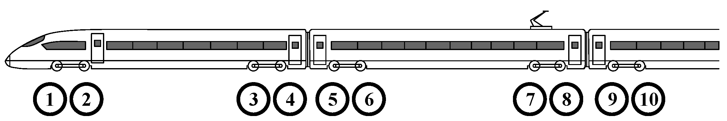
Consider the multiple-unit railroad vehicle illustrated in Figure 1. Its traction system is distributed across the entire vehicle, eliminating the need for a traditional locomotive [19]. Electric motors power the driven axles, which are located at positions ➀, ➃, ➄, ➇, and ➈ in various carriages. Replacing non-driven axles with driven ones is often considered an effective method to increase a train’s maximum speed, introducing identical input redundancy. However, according to physical laws, the theoretical maximum drag force (TMDF) of a vehicle is determined by its weight multiplied by the friction coefficient between the wheels and the rail. The TMDF serves as an upper limit for the total driving force, with the vehicle’s weight and friction coefficient remaining constant. With a limited number of driven axles and relatively small, powerful motors, the total driving force will likely be far less than the TMDF. In this scenario, adding new input redundancy may actually decrease the optimal time. Conversely, if more powerful motors are added, the total driving force can approach and maintain the TMDF. In this case, introducing additional input redundancy will not reduce the optimal time. As a result, the input constraint subtly shifts from $\Pi$ to $\Theta$, which will be defined and discussed in subsequent sections of this paper.

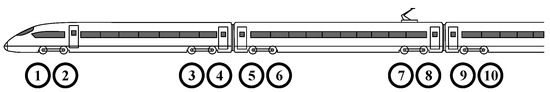
Figure 1. Multiple-unit railroad vehicle with identical input redundancies.

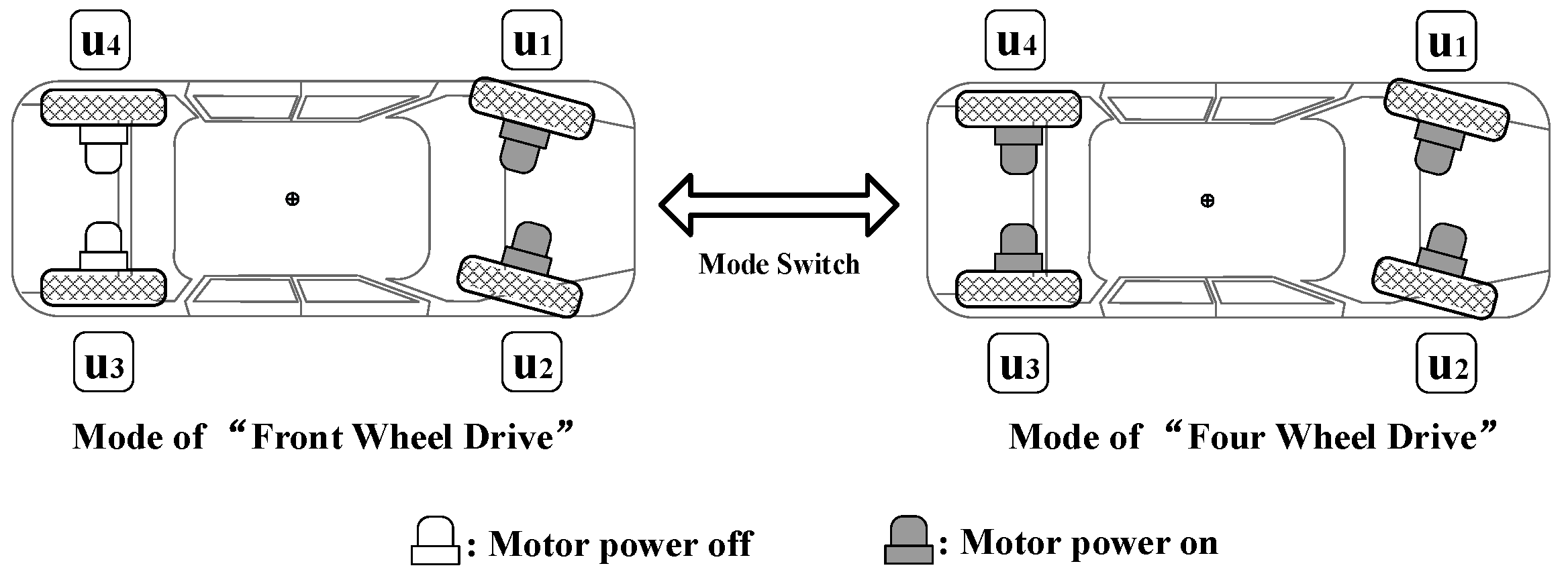
Now, let us examine a sports utility vehicle (SUV) powered by electric motors, as shown in Figure 2. This SUV has two drive modes: front-wheel drive and four-wheel drive. In front-wheel drive mode, the driving force is generated by the two front wheels (motors), denoted as $u_1$ and $u_2$. In contrast, all four motors are utilized to propel the vehicle in four-wheel drive mode. The following expression is employed to describe the SUV:

$$\begin{array}{c}\hfill \dot{x}=Ax+\tilde{B}W\tilde{u},\end{array}$$

(1)

where $A\in {\mathbb{R}}^{n\times n}$, $\tilde{B}=[B,B_{\alpha }]\in {\mathbb{R}}^{n\times 4}$, $B\in {\mathbb{R}}^{n\times 2}$, $B_{\alpha }\in {\mathbb{R}}^{n\times 2}$, $W=diag\{w_1,w_2,w_3,w_4\}\in {\mathbb{R}}^{4\times 4}$, $\tilde{u}={[u^T,u_{\alpha }^T]}^T={[u_1,u_2,u_3,u_4]}^T\in {\mathbb{R}}^4$, $u={[u_1,u_2]}^T\in {\mathbb{R}}^2$, and $u_{\alpha }={[u_3,u_4]}^T\in {\mathbb{R}}^2$. In front-wheel drive mode, the matrix W satisfies $W=W_{front}=diag\{1,1,0,0\}$ with no input redundancy, and system (1) becomes

$$\begin{array}{c}\hfill \dot{x}=Ax+Bu.\end{array}$$

(2)

In four-wheel drive mode, we have $W=W_{four}=diag\{1,1,1,1\}$, and then system (1) with different input redundancies becomes

$$\begin{array}{c}\hfill \dot{x}=Ax+\left[B{B}_{\alpha }\right]\tilde{u}.\end{array}$$

(3)

Similar to the multiple-unit railroad vehicle, the effect of adding these new input redundancies to the SUV vehicle depends on its TMDF, which means its input constraint may shift from $\Pi$ to $\Theta$.

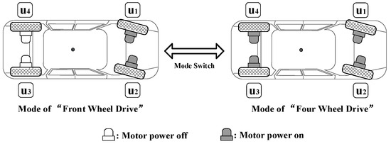
Figure 2. Sports utility vehicle powered by different electric motors.

The impact of input redundancy in these two examples might seem straightforward, but they serve as an inspiration for understanding the general principles that apply to more complex scenarios. With the rapid advancement of science and technology, a plethora of new types of actuators have become available. Consequently, it is an essential task for system designers to ascertain which actuators and how many are necessary to achieve improved performance. Undoubtedly, theoretical insights can greatly benefit this endeavor. Our paper concentrates on establishing theoretical results that guarantee a reduction in time-optimal control problems with input redundancy in both linear and nonlinear systems.

This paper is organized as follows. Section 2.1 introduces the concept of a non-idle channel to represent the input channel, highlighting that its presence among input redundancies can lead to a decrease in the optimal time. In Section 2.2, input constraints are classified into two categories: degenerate and nondegenerate. For nondegenerate constraints, the inherent normality of the problem ensures a reduction in the optimal time due to input redundancy. Conversely, this reduction is not guaranteed for degenerate constraints. Section 2.3 discusses identical input redundancy, where the extent of reduction depends on the types of input constraints. Section 2.4 examines the impact of adding new input redundancy in linear time-invariant (LTI) systems, relating it to system controllability. Section 3 utilizes two numerical examples to substantiate our theoretical findings. Finally, Section 4 presents the conclusions of this study.

2. Materials and Methods

This section details our theoretical results, which assert that the incorporation of input redundancy facilitates faster time-optimal control in both affine nonlinear systems and linear systems.

2.1. Affine Nonlinear Systems with Input Redundancy

Preliminarily, we delineate the time-optimal control problem for affine nonlinear systems without input redundancy as follows:

Problem 1.

Minimize the final time, $T\left(x_0\right)={\int }_0^{T}dt$, required to transfer the affine nonlinear system

$$\begin{array}{c}\hfill \dot{x}\left(t\right)=f(x\left(t\right),t)+Bu\left(t\right),\end{array}$$

(4)

from a nonzero initial state $x_0\in {\mathbb{R}}^n$ to the origin point $x\left(T\left(x_0\right)\right)=0$, where $B\in {\mathbb{R}}^{n\times r}$, $u\left(t\right)\in {\mathcal{U}}_r$, and ${\mathcal{U}}_r$ is an r-dimensional bounded closed set.

Now, we consider the transformation of the above problem when input redundancy is incorporated, as follows:

Problem 2.

Minimize the final time, $\tilde{T}\left(x_0\right)$, within which the redundant affine nonlinear system

$$\begin{array}{c}\hfill \dot{\tilde{x}}\left(t\right)=f(\tilde{x}\left(t\right),t)+\tilde{B}\tilde{u}\left(t\right),\end{array}$$

(5)

can be transferred from a nonzero initial state $x_0\in {\mathbb{R}}^n$ to the origin point, where $\tilde{B}=\left[B{B}_{\alpha }\right]\in {\mathbb{R}}^{n\times (r+k)}$ and $B_{\alpha }\in {\mathbb{R}}^{n\times k}$, $\tilde{u}\left(t\right)={[u^T\left(t\right),u_{\alpha }^T\left(t\right)]}^T\in {\mathcal{U}}_{r+k}$, $u\left(t\right)\in {\mathcal{U}}_r$, ${\mathcal{U}}_{r+k}$ is an $(r+k)$-dimensional bounded closed set that satisfies ${\mathcal{U}}_{r+k}⊋{\mathcal{U}}_{r+0\left(k\right)}$, where

$$\begin{array}{c}\hfill {\mathcal{U}}_{r+0\left(k\right)}:=\left\{\tilde{u}\in {\mathbb{R}}^{r+k}\left|\tilde{u}=\left[\begin{array}{c}u\hfill \\ 0\hfill \end{array}\right],\mathit{where}u\in {\mathcal{U}}_r\subseteq {\mathbb{R}}^r\right.\right\}.\end{array}$$

(6)

Let ${\tilde{T}}^{*}\left(x_0\right)$ and $T^{*}\left(x_0\right)$ denote the optimal times for the control problems with and without input redundancy, respectively, starting from the initial state $x_0$. Given that ${\mathcal{U}}_{r+k}$ constitutes a proper superset of ${\mathcal{U}}_{r+0\left(k\right)}$ (i.e., ${\mathcal{U}}_{r+k}⊋{\mathcal{U}}_{r+0\left(k\right)}$), it follows that the optimal time must satisfy ${\tilde{T}}^{*}\left(x_0\right)⩽T^{*}\left(x_0\right)$ for any initial state $x_0$. However, it is not inherently guaranteed that a strict reduction occurs such that ${\tilde{T}}^{*}\left(x_0\right)<T^{*}\left(x_0\right)$. To illustrate a scenario where the optimal time remains unaltered despite the introduction of input redundancy, consider Problem 1 with the following system description:

$$\begin{array}{c}\hfill \dot{x}\left(t\right)=u\left(t\right),\end{array}$$

(7)

where $u\left(t\right)\in {\mathcal{U}}_1=\left\{u\left(t\right)\in \mathbb{R}:-1⩽u\left(t\right)⩽1\right\}$. Meanwhile, consider Problem 2 with the following system with redundancy:

$$\begin{array}{c}\hfill \dot{\tilde{x}}\left(t\right)=\tilde{B}\tilde{u}\left(t\right)=u\left(t\right)+u_{\alpha }\left(t\right),\end{array}$$

(8)

where $\tilde{u}\left(t\right)\in {\mathcal{U}}_2=\left\{{\left(u\left(t\right),u_{\alpha }\left(t\right)\right)}^T\in {\mathbb{R}}^2{:\left|\right|u\left(t\right)\left|\right|}_1+\left|\right|u_{\alpha }{\left|\right|}_1⩽1\right\}$. Then, their optimal time will always be identical to

$$\begin{array}{c}\hfill T^{*}\left(x_0\right)=\left|\right|x_0{\left|\right|}_1={\tilde{T}}^{*}\left(x_0\right),\end{array}$$

(9)

throughout the entire state space. Equation (9) indicates that the presence of input redundancy does not reduce the optimal time; an explanation for this occurrence is provided in Section 2.3. Now, we introduce the definitions of idle and non-idle channels.

Definition 1.

Input channel $u_i\left(t\right)\in {\mathbb{R}}^1$ is called an “idle channel with respect to $x_0$” if this channel is unused during the entire optimal time interval with respect to $x_0\ne 0$, where $i\in \{1,\cdots ,d(u\left)\right\}$ and $d\left(u\right)$ represents the dimension of the input vector $u\left(t\right)$.

Definition 2.

Input channel $u_i\left(t\right)\in {\mathbb{R}}^1$ is called a “non-idle channel with respect to $x_0$” if the optimal control input of this channel is nonzero during at least one nontrivial time interval $[t_1,t_2]\subset [0,{\tilde{T}}^{*}\left(x_0\right)]$ with respect to $x_0\ne 0$, where nontrivial means $t_1\ne t_2$.

Then, a sufficient condition can be derived to ascertain the strict reduction in the optimal time following the addition of input redundancy.

Theorem 1.

Suppose there exists an optimal control for Problems 1 and 2, and that the optimal control for Problem 2 is unique. Then, the optimal time satisfies

$$\begin{array}{c}\hfill {\tilde{T}}^{*}\left(x_0\right)<T^{*}\left(x_0\right),\end{array}$$

(10)

for any initial state $x_0\ne 0$, provided that Problem 2 features a non-idle redundant channel with respect to $x_0\ne 0$.

Proof. 

For $x_0\ne 0$, assume that ${\tilde{u}}_i^{*}\left(t\right)\in {\mathbb{R}}^1$ is a non-idle redundant channel, where $i\in \{r+1,\cdots ,r+k\}$. According to Definition 2, there exists a nontrivial time interval $[t_1,t_2]\subset [0,{\tilde{T}}^{*}\left(x_0\right)]$ such that ${\tilde{u}}_i^{*}\left(\xi \right)\ne 0$, where $\xi \in [t_1,t_2]$. Then, the optimal control satisfies

$$\begin{array}{c}\hfill {\tilde{u}}^{*}\left(\xi \right)={[u_1^{*}\left(\xi \right),\cdots ,u_r^{*}\left(\xi \right),\cdots ,u_i^{*}\left(\xi \right),\cdots ]}^T\ne {[u_1^{*}\left(\xi \right),\cdots ,u_r^{*}\left(\xi \right),0,\cdots ,0]}^T={[u^T\left(\xi \right),0]}^T,\end{array}$$

(11)

where no feasible control for Problem 1 can form the unique optimal control ${\tilde{u}}^{*}\left(t\right)$ for Problem 2. As a result, the optimal time will strictly reduce.    □

Nevertheless, demonstrating the existence of a non-idle redundant channel does not depend on the uniqueness of the optimal control for Problem 2. Consequently, we arrive at the following theorem:

Theorem 2.

If the optimal time for Problems 1 and 2 satisfies

$$\begin{array}{c}\hfill {\tilde{T}}^{*}\left(x_0\right)<T^{*}\left(x_0\right),\end{array}$$

(12)

with respect to $x_0\ne 0$, then there exists a non-idle channel among the input redundancies.

Proof. 

This can be proven by contradiction. Firstly, assume that all the redundant channels are idle for $x_0$. Then, there exists $u_{\beta }\left(t\right)\in {\mathcal{U}}_r$ that forms ${[u_{\beta }^T\left(t\right),0]}^T={\tilde{u}}^{*}\left(t\right)$ as the optimal control for Problem 2 with ${\tilde{T}}^{*}\left(x_0\right)$. Let the control for Problem 1 be $u\left(t\right)=u_{\beta }\left(t\right)$. Then, we obtain $T_{\beta }\left(x_0\right)={\tilde{T}}^{*}\left(x_0\right)$. This further means $T^{*}\left(x_0\right)⩽{\tilde{T}}^{*}\left(x_0\right)$ since $T^{*}\left(x_0\right)⩽T_{\beta }\left(x_0\right)$. This contradicts the precondition that ${\tilde{T}}^{*}\left(x_0\right)<T^{*}\left(x_0\right)$. Thus, there must exist a non-idle redundant channel if ${\tilde{T}}^{*}\left(x_0\right)<T^{*}\left(x_0\right)$.    □

Remark 1.

Theorem 1 serves as a sufficient condition, ensuring that the addition of input redundancy will lead to a reduction in the optimal time, whereas Theorem 2 provides a necessary condition for the same effect.

In accordance with Theorem 1, it is imperative to ascertain the optimal time for every initial state in order to formulate a comprehensive assessment of input redundancy across the entire state space. However, for subsequent analysis, knowledge of the optimal time for states on a lower-dimensional hypersurface of $\partial M$ suffices.

Theorem 3.

Let M be a bounded closed set and $M^c$ be its complement in the state space ${\mathcal{X}}_n$, where the origin is an interior point of M and $\partial M$ represents its boundary. Then, the optimal time satisfies

$$\begin{array}{c}\hfill {\tilde{T}}^{*}\left(x_0\right)<T^{*}\left(x_0\right),\end{array}$$

(13)

for all $x_0\in M^c$ if every $x_0\in \partial M$ experiences a reduction in the optimal time after adding input redundancy.

Pursuant to Theorem 3, if all states on the boundary exhibit a reduced optimal time due to input redundancy, then any state exterior to this boundary will also experience a reduced optimal time. To elucidate this theorem, consider the set $M\in {\mathcal{X}}_2={\mathbb{R}}^2$, as illustrated in Figure 3. As depicted, the boundary of M is denoted by $\partial M$, which is encircled by the smallest circle $c_1$. For an initial state $x_0=a$ located outside M, the optimal trajectory without input redundancy comprises segments $l_0$ and $l_1$, intersecting at point $b\in \partial M$. When input redundancy is employed, the optimal trajectory originating from $x_0=b$ is $l_2$. If ${\tilde{T}}_{l_2}^{*}\left(b\right)<T_{l_1}^{*}\left(b\right)$, we have

$$\begin{array}{c}\hfill {\tilde{T}}^{*}\left(a\right)⩽T_{l_0}^{*}\left(a\right)+{\tilde{T}}_{l_2}^{*}\left(b\right)<T_{l_0}^{*}\left(a\right)+T_{l_1}^{*}\left(b\right)=T^{*}\left(a\right).\end{array}$$

(14)

Consequently, if every state on $\partial M$ exhibits a reduced optimal time with the introduction of input redundancy, it follows that all states outside $\partial M$ will do so as well. Furthermore, by applying Algorithm 1, the radius of $c_2$ can be made to approximate that of $c_1$.

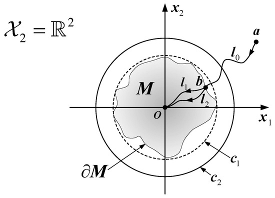
Figure 3. A closed set M in the state space ${\mathcal{X}}_2={\mathbb{R}}^2$.

For the sake of computational simplicity, we use the hypersphere

$$\begin{array}{c}\hfill \partial S\left(r\right):=\left\{x\in {\mathbb{R}}^n{\left|\right|\left|x\right||}_2=r,r>0\right\},\end{array}$$

(15)

to replace $\partial M$ in Theorem 3. Let $r_{min}$ denote the minimum radius such that the optimal time decreases for every $\left|\right|x_0{\left|\right|}_2⩾r_{min}$. Evidently, if $r_{min}=0$, the entire state space, except for the origin point, will undergo a reduction in the optimal time when input redundancy is introduced. Conversely, any $\delta >0$ that satisfies $r_{min}-\delta >0$ will yield ${\tilde{T}}^{*}\left(x_0\right)=T^{*}\left(x_0\right)$ for certain $x_0\in \partial S\left(\delta \right)$. Typically, $r_{min}$ is an unknown priori, which can be calculated by implementing the algorithm below.

Algorithm 1: The approximation of $r_{min}$

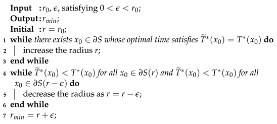2.2. Redundancy in Nondegenerate and Degenerate Input Constraints

It is well established that for a normal time-optimal control Problem 2, the control ${\tilde{u}}^{*}\left(t\right)$ will be a bang-bang control, residing on the boundary $\partial {\mathcal{U}}_{r+k}$. The term “normal” implies that ${\tilde{u}}^{*}\left(t\right)$ can be determined by the Hamiltonian throughout any nontrivial time interval. It should be noted that the discussions in this subsection pertain to behaviors during nontrivial time intervals, which may not hold true at isolated points in time. Within the context of a normal problem, both nondegenerate and degenerate input constraints are considered.

Definition 3.

An input constraint ${\mathcal{U}}_{r+k}$ is nondegenerate if ${\mathcal{Z}}_{r+k}\cap {\mathcal{W}}_{r+k}^c=\varnothing$, where

$$\begin{array}{c}\hfill {\mathcal{Z}}_{r+k}:=\left\{z\in \partial {\mathcal{U}}_{r+k}|z^{T}z>z^T\tilde{u},\mathit{for}\mathit{every}\tilde{u}\in \partial {\mathcal{U}}_{r+k}\mathit{except}z\right\},\end{array}$$

(16)

and ${\mathcal{W}}_{r+k}^c$ represents the complement of ${\mathcal{W}}_{r+k}$ in ${\mathcal{U}}_{r+k}$, where

$$\begin{array}{c}\hfill {\mathcal{W}}_{r+k}:=\left\{w\in \partial {\mathcal{U}}_{r+k}\left|w=\left[\begin{array}{c}{w}_1\\ ⋮\\ w_{r+k}\end{array}\right],\mathit{satisfying}{w}_i\ne 0\mathit{for}\mathit{every}i=1,\cdots ,r+k\right.\right\}.\end{array}$$

(17)

Definition 4.

An input constraint ${\mathcal{U}}_{r+k}$ is degenerate if there exists $z\in {\mathcal{Z}}_{r+k}$ such that $z\notin {\mathcal{W}}_{r+k}$.

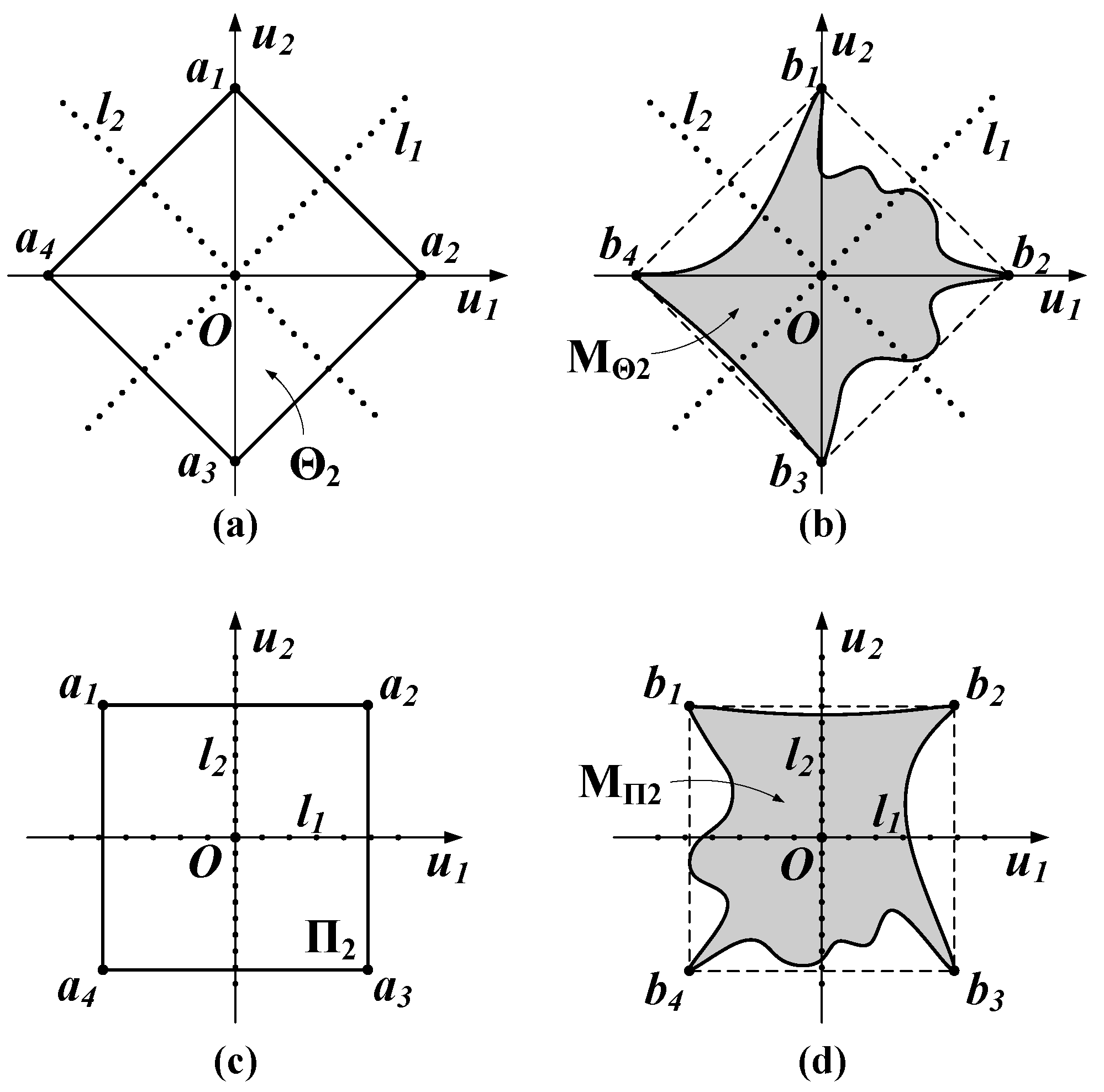
Illustrative examples of degenerate and nondegenerate input constraints are presented in Figure 4. It is evident that both degenerate and nondegenerate input constraints can be nonconvex, as demonstrated by ${\mathrm{M}}_{{\Theta }_2}$ and ${\mathrm{M}}_{{\Pi }_2}$, respectively.

Figure 4. Examples of degenerate and nondegenerate input constraints in ${\mathbb{R}}^2$: (a) degenerate convex set ${\Theta }_2$; (b) degenerate nonconvex set ${\mathrm{M}}_{{\Theta }_2}$; (c) nondegenerate convex set ${\Pi }_2$; (d) nondegenerate nonconvex set ${\mathrm{M}}_{{\Pi }_2}$.

Evidently, for a normal problem, its optimal control will adhere to the condition ${\tilde{u}}^{*}\in {\mathcal{Z}}_{r+k}$. Furthermore, when the optimal control is a member of ${\mathcal{W}}_{r+k}$, it signifies that all input channels are active. Consequently, for a normal Problem 2 that features nondegenerate input constraints, not a single redundant channel remains idle. A well-known example of a nondegenerate input constraint is ${\Pi }_{d\left(u\right)}$, which is defined as

$$\begin{array}{c}\hfill {\Pi }_{d\left(u\right)}:=\left\{u\left(t\right):[0,+\infty )\to {\mathbb{R}}^{d\left(u\right)}\left|\right||u_i\left(t\right){\left|\right|}_1⩽1\mathrm{for}\mathrm{every}i=1,\cdots ,d\left(u\right)\right\}.\end{array}$$

(18)

However, the input constraints of ${\Phi }_{d\left(u\right)}$ and ${\Theta }_{d\left(u\right)}$ are degenerate, which are defined as follows:

$$\begin{array}{c}\hfill {\Phi }_{d\left(u\right)}:=\left\{u\left(t\right):[0,+\infty )\mapsto {\mathbb{R}}^{d\left(u\right)}{\left|\right|\left|u\left(t\right)\right||}_2⩽1\right\},\end{array}$$

(19)

and

$$\begin{array}{c}\hfill {\Theta }_{d\left(u\right)}:=\left\{u\left(t\right):[0,+\infty )\mapsto {\mathbb{R}}^{d\left(u\right)}\left|\sum _{i=1}^{d\left(u\right)}\left|\right|u_i\left(t\right){\left|\right|}_1⩽1\right.\right\}.\end{array}$$

(20)

Referring back to the systems in (7) and (8), it is evident that their input constraints correspond to the degenerate case of ${\Theta }_{d\left(u\right)}$.

Given that the optimal control for a normal problem is uniquely determined by the Hamiltonian, its existence inherently ensures its uniqueness. According to Theorem 1, the following result can be readily deduced:

Corollary 1.

Suppose the existence of optimal controls for Problem 1 and Problem 2. If ${\mathcal{U}}_{r+k}$ is nondegenerate and Problem 2 is normal, then the optimal time satisfies

$$\begin{array}{c}\hfill {\tilde{T}}^{*}\left(x_0\right)<T^{*}\left(x_0\right),\end{array}$$

(21)

for any nonzero initial state $x_0$.

Proof. 

If ${\mathcal{U}}_{r+k}$ is nondegenerate and Problem 2 is normal, then ${\tilde{u}}^{*}\left(t\right)\in \partial {\mathcal{U}}_{r+k}$ and ${\tilde{u}}^{*}\left(t\right)\notin \partial ({\mathcal{U}}_r\oplus \left\{0\right\})\cap \partial {\mathcal{U}}_{r+k}$, which means that all of the input channels (including the redundant input channels) are non-idle channels in the optimal control for Problem 2 from any nonzero initial state. According to Theorem 1, it can be concluded that ${\tilde{T}}^{*}\left(x_0\right)<T^{*}\left(x_0\right)$. □

However, in the presence of degenerate input constraints, input redundancy does not lead to an improvement in the optimal time. To illustrate this, we consider the ${\Theta }_{d\left(u\right)}$ constraint and construct two novel problems as outlined below.

Problem 3.

Problem 1, except that the input constraint becomes ${\Theta }_r$.

Problem 4.

Problem 2, except that the input constraint becomes ${\Theta }_{r+k}$.

Given that both ${\Theta }_r$ and ${\Theta }_{r+k}$ are bounded closed sets, the conclusions derived from the preceding subsection remain applicable to these two newly formulated problems.

The Hamiltonian of Problem 2 or Problem 4 is

$$\begin{array}{c}\hfill \tilde{H}(\tilde{x}\left(t\right),\tilde{\lambda }\left(t\right),\tilde{u}\left(t\right),t)=1+{\tilde{\lambda }}^T\left(t\right)f(\tilde{x}\left(t\right),t)+{\tilde{\lambda }}^T\left(t\right)\tilde{B}\tilde{u}\left(t\right),\end{array}$$

(22)

where $\tilde{\lambda }\left(t\right):[0,T]\to {\mathbb{R}}^n$ is called a costate vector. According to Pontryagin’s Maximum Principle (PMP) [20], the minimum of (22) satisfies

$$\begin{array}{c}\hfill \underset{\tilde{u}\in {\mathcal{U}}_{r+k}}{min}\tilde{H}⟺\underset{\tilde{u}\in {\mathcal{U}}_{r+k}}{min}\left\{{\tilde{\lambda }}^T\left(t\right)\tilde{B}\tilde{u}\left(t\right)\right\}=\underset{\tilde{u}\in {\mathcal{U}}_{r+k}}{min}\left\{{\tilde{q}}_1^T\left(t\right){\tilde{u}}_1\left(t\right)+\cdots +{\tilde{q}}_{r+k}^T\left(t\right){\tilde{u}}_{r+k}\left(t\right)\right\},\end{array}$$

(23)

where ${\tilde{q}}_j\left(t\right):={\tilde{b}}_j^T\tilde{\lambda }\left(t\right)$, $j=1,\cdots ,r+k$, ${\tilde{b}}_j$ is the j-th column of input matrix $\tilde{B}$. The vector $\tilde{q}\left(t\right)\in {\mathbb{R}}^{r+k}$ is called a switching vector. The normality of Problem 4 is defined as follows:

Definition 5

([21]). Problem 4 is normal if and only if one component ${\tilde{q}}_l\left(\zeta \right)\in {\mathbb{R}}^1$ of $\tilde{q}\left(\zeta \right)\in {\mathbb{R}}^{r+k}$ reaches the extreme value during any nontrivial time interval $[t_1,t_2]\subset [0,{\tilde{T}}^{*}]$, i.e., $|{\tilde{q}}_l\left(\zeta \right)|>|{\tilde{q}}_j\left(\zeta \right)|$ for every $j=1,\cdots ,r+k$ other than l, where $\zeta \in [t_1,t_2]$ and $l\in \{1,\cdots ,r+k\}$.

According to (23) and Definition 5, the optimal control for Problem 4 is called dynamic single-input control (DSIC) [21], where only one input channel works at its extreme value while all the other ones are unused. Additionally, the working channel may switch among different channels during different time intervals. Clearly, if Problem 4 is normal but none of the redundant channels is the working channel, the optimal time will not reduce after adding input redundancy.

2.3. The Effect of Adding Identical Input Redundancy

When employing identical input redundancy, the input matrix transforms into $\tilde{B}=[B,B]$, a scenario commonly encountered in life-critical systems, as discussed in the previous section. Intuitively, duplicating actuators appears to bolster system capabilities, presumably leading to a decrease in the optimal time. Nonetheless, the impact of introducing identical input redundancy is contingent on the nature of the input constraint in place.

Firstly, a system with identical input redundancy can be formulated as follows:

$$\begin{array}{c}\hfill \dot{\tilde{x}}\left(t\right)=f(\tilde{x}\left(t\right),t)+[B,B]\tilde{u}\left(t\right),\end{array}$$

(24)

where $\tilde{u}\left(t\right)={[u_{\zeta }^T\left(t\right),u_{\xi }^T\left(t\right)]}^T\in {\mathcal{U}}_{2r}$ and $u_{\zeta }\left(t\right)$, $u_{\xi }\left(t\right)\in {\mathcal{U}}_r$. It is evident that input control can be distributed arbitrarily between $u_{\zeta }\left(t\right)$ and $u_{\xi }\left(t\right)$ without affecting system dynamics. Assuming $u_{\zeta }\left(t\right)=u_{\xi }\left(t\right)$, system (24) becomes

$$\begin{array}{c}\hfill \dot{x}\left(t\right)=f(x\left(t\right),t)+B\left(u_{\zeta }\left(t\right)+u_{\xi }\left(t\right)\right)=f(x\left(t\right),t)+2·B{u}_{\gamma }\left(t\right),\end{array}$$

(25)

where $u_{\gamma }\left(t\right)=u_{\zeta }\left(t\right)=u_{\xi }\left(t\right)$.

According to PMP, the terminal value of $\lambda \left(t\right)$ in Problem 1 should fulfill the following equation [22]:

$$\begin{array}{c}\hfill 1+{\lambda }^T\left(T^{*}\right)f(x\left(T^{*}\right),T^{*})+{\lambda }^T\left(T^{*}\right)Bu\left(T^{*}\right)=0.\end{array}$$

(26)

Because $\lambda \left(T^{*}\right)=0$ leads to $1=0$ in (26), $\lambda \left(T^{*}\right)$ should be nonzero. If the origin point is an equilibrium of (24), then $f(0,t)=0$. As a result, $x\left(T^{*}\right)=0$ leads to $1+{\lambda }^T\left(T^{*}\right)Bu\left(T^{*}\right)=0$ in (26), which means $\left|\right|{\lambda }^T\left(T^{*}\right){\left|\right|}_1<+\infty$ under the constrained $u\left(T^{*}\right)$. Meanwhile, since [22]

$$\begin{array}{c}\hfill \dot{\lambda }\left(t\right)=-{\displaystyle \frac{\partial f^T(x\left(t\right),t)}{\partial x}}\lambda \left(t\right),\end{array}$$

(27)

it can be deduced that ${\left|\right|\lambda \left(t\right)\left|\right|}_1<+\infty$ and $\left|\right|\dot{\lambda }\left(t\right){\left|\right|}_1<+\infty$ for all $t⩽T^{*}$. Consequently, there exists a $0<ϵ⩽T^{*}$ such that $\lambda \left(t\right)\ne 0$ for $t\in [T^{*}-ϵ,T^{*}]$. This implies that the corresponding optimal control assumes a bang-bang form during the interval $t\in [T^{*}-ϵ,T^{*}]$, leading to the following theorem:

Theorem 4.

Suppose the existence of the optimal control for Problem 1 with input constraints ${\mathcal{M}}_r$ and ${\mathcal{N}}_r$. Then, the optimal time satisfies

$$\begin{array}{c}\hfill T_{{\mathcal{N}}_r}^{*}\left(x_0\right)<T_{{\mathcal{M}}_r}^{*}\left(x_0\right),\end{array}$$

(28)

for every $x_0\ne 0$ if ${\mathcal{M}}_r\subset {\stackrel{\circ }{\mathcal{N}}}_r$, where ${\mathcal{M}}_r$ and ${\mathcal{N}}_r$ are two bounded closed sets, and ${\stackrel{\circ }{\mathcal{N}}}_r$ represents the interior of set ${\mathcal{N}}_r$.

In order to gain an insight into this theorem, let us examine the input constraint for $u_{\gamma }\left(t\right)$ within system (25).

On the one hand, if ${\mathcal{U}}_{2r}$ is equivalently substitutable by $u_{\zeta }\left(t\right)\in {\mathcal{U}}_r$ and $u_{\xi }\left(t\right)\in {\mathcal{U}}_r$ within (24), the input constraint for (25) would then be $u_{\gamma }\left(t\right)\in {\mathcal{U}}_r$. Moreover, system (24) would be equivalent to system (4), albeit with an expanded constraint set such that $u\left(t\right)\in 2{\mathcal{U}}_r\supset {\mathcal{U}}_r$. In accordance with Theorem 4, given that $2{\mathcal{U}}_r⊋{\mathcal{U}}_r$, the optimal time is guaranteed to decrease strictly upon the addition of identical input redundancy. Clearly, ${\Pi }_{d\left(u\right)}$ is an example that falls under this category of input constraints.

On the other hand, if the replacement of $\tilde{u}\left(t\right)\in {\mathcal{U}}_{2r}$ with $u_{\zeta }\left(t\right)\in {\mathcal{U}}_r$ and $u_{\xi }\left(t\right)\in {\mathcal{U}}_r$ is not viable, the impact of introducing identical input redundancy would vary according to the specific type of input constraint. To illustrate this point, we consider the examples of ${\Theta }_{d\left(u\right)}$ and ${\Phi }_{d\left(u\right)}$. According to (25), if $\tilde{u}\left(t\right)\in {\Theta }_{2r}$, the input constraint in (24) becomes

$$\begin{array}{cc}\hfill {\Theta }_{2r}& \Rightarrow \left\{\tilde{u}\left(t\right)={[u_{\zeta }^T\left(t\right),u_{\zeta }^T\left(t\right)]}^T\in {\mathbb{R}}^{2r},\mathrm{where}\sum _{i=1}^r\left(\left|\right|u_{\zeta i}{\left(t\right)\left|\right|}_1+\left|\right|u_{\zeta i}\left(t\right){\left|\right|}_1\right)⩽1\right\}\hfill \\ \hfill & \Rightarrow \left\{\tilde{u}\left(t\right)={[u_{\zeta }^T\left(t\right),u_{\zeta }^T\left(t\right)]}^T\in {\mathbb{R}}^{2r},\mathrm{where}\sum _{i=1}^r\left|\right|u_{\zeta i}\left(t\right){\left|\right|}_1⩽{\displaystyle \frac{1}{2}}\right\}.\hfill \end{array}$$

(29)

Furthermore, the input constraint in (25) becomes

$$\begin{array}{c}\hfill \left\{u_{\gamma }\left(t\right)\in {\mathbb{R}}^r,\mathrm{where}\sum _{i=1}^r\left|\right|u_{\gamma i}\left(t\right){\left|\right|}_1⩽{\displaystyle \frac{1}{2}}\right\}\Rightarrow {\displaystyle \frac{1}{2}}{\Theta }_r.\end{array}$$

(30)

In accordance with (9), the optimal time remains invariant when identical input redundancy is introduced.

Conversely, when considering $\tilde{u}\left(t\right)\in {\Phi }_{2r}$, the input redundancy in (24) and (25) results in a constraint that transforms into

$$\begin{array}{c}\hfill \sqrt{{\displaystyle \sum _{i=1}^r}\left(u_{\zeta i}^2\left(t\right)+u_{\xi i}^2\left(t\right)\right)}⩽1\Rightarrow \sqrt{{\displaystyle \sum _{i=1}^r}{u}_{\gamma i}^2\left(t\right)}⩽{\displaystyle \frac{\sqrt{2}}{2}}\Rightarrow 2u_{\gamma }\left(t\right)\in \sqrt{2}{\Phi }_r.\end{array}$$

(31)

Pursuant to Theorem 4, given that ${\Phi }_r⊊\sqrt{2}{\Phi }_r$, it follows that the optimal time will exhibit a decrease when identical input redundancy is introduced.

2.4. Input Redundancy in LTI Systems

It is a well-established fact that a linear time-invariant (LTI) system is controllable if and only if its controllability matrix

$$\begin{array}{c}\hfill \mathcal{C}=[B,AB,\cdots ,A^{n-1}B]\end{array}$$

(32)

possesses full row rank [23]. Evidently, within the realm of LTI systems, once a system is deemed controllable, its controllability remains invariant even after the introduction of input redundancy. Nevertheless, as elucidated in this subsection, the optimal time associated with the system is subject to reduction upon the addition of input redundancy. First, we formulate the time-optimal control problem for the LTI system as follows:

Problem 5.

Minimize the final time $T\left(x_0\right)={\int }_0^{T}dt$ to transfer the LTI system

$$\begin{array}{c}\hfill \dot{x}\left(t\right)=Ax\left(t\right)+Bu\left(t\right),\end{array}$$

(33)

from an initial state $x_0\ne 0$ to the origin point of 0, where $A\in {\mathbb{R}}^{n\times n}$ and $B\in {\mathbb{R}}^{n\times r}$, $u\left(t\right)\in {\Pi }_r$ is Lebesgue measurable.

Meanwhile, the LTI system with input redundancy has the following time-optimal control problem:

Problem 6.

Minimize the final time, $\tilde{T}\left(x_0\right)$, to transfer the redundant LTI system

$$\begin{array}{c}\hfill \dot{\tilde{x}}\left(t\right)=A\tilde{x}\left(t\right)+\tilde{B}\tilde{u}\left(t\right),\end{array}$$

(34)

from an initial state $x_0\ne 0$ to the origin point of 0, where $\tilde{B}=\left[B{B}_1\right]\in {\mathbb{R}}^{n\times (r+k)}$ and $B_1\in {\mathbb{R}}^{n\times k}$, $\tilde{u}\left(t\right)\in {\Pi }_{r+k}$ is Lebesgue measurable.

In system (33), the dynamics of its state can be explicitly formulated as follows:

$$\begin{array}{c}\hfill x\left(t\right)=e^{At}{x}_0+{\int }_0^t{e}^{A(t-s)}Bu\left(s\right)ds.\end{array}$$

(35)

Since $x\left(T\left(x_0\right)\right)=0$, we have

$$\begin{array}{c}\hfill x_0=-{\int }_0^T{e}^{-As}Bu\left(s\right)ds,\end{array}$$

(36)

which defines a bounded linear mapping

$$\begin{array}{c}\hfill x_0=\phi \left(u\left(s\right)\right).\end{array}$$

(37)

According to [24], an operator between two normed spaces is a bounded linear operator if and only if it is a continuous linear operator. Since a continuous linear operator maps a bounded set into a bounded set, then we can conclude that

$$\begin{array}{c}\hfill \Omega \left(t\right)=\phi \left({\Pi }_r\right)\end{array}$$

(38)

is bounded. From any initial state $x_0\in \Omega \left(t\right)$, there always exists a control $u\left(t\right)\in {\Pi }_r$ to transfer system (33) to the origin point 0 within time t. Similarly, there exists a bounded linear mapping $\tilde{\phi }(·)$ for the redundant system (34), which can be expressed as follows:

$$\begin{array}{c}\hfill \tilde{\Omega }\left(t\right)=\tilde{\phi }\left({\Pi }_{r+k}\right).\end{array}$$

(39)

In the redundant system (34), its controllability satisfies the following:

Lemma 1

([20,22]). Time-optimal control ${\tilde{u}}^{*}\left(t\right)$ exists for every $x_0\in \tilde{\Omega }\left(t\right)$ in Problem 6 if the pair $(A,\tilde{B})$ is controllable, where $\tilde{\Omega }\left(t\right)$ is defined in (39).

Meanwhile, the following lemma reveals the relationship between non-idle channels and the controllability of redundant LTI systems.

Lemma 2.

If $(A,b_i)$ is controllable, then $u_i^{*}\left(t\right)$ is a non-idle channel with respect to any initial state $x_0\ne 0$, where $b_i$ represents the i-th column of B.

Proof. 

According to PMP, the minimum of the Hamiltonian satisfies

$$\begin{array}{c}\hfill \underset{u\in {\Pi }_r}{min}H⟺\underset{u\in {\Pi }_r}{min}\left\{{\lambda }^T\left(t\right)Bu\left(t\right)\right\}.\end{array}$$

(40)

Meanwhile, $\dot{\lambda }\left(t\right)=-A^T\lambda \left(t\right)$ results in $\lambda \left(t\right)=e^{-A^{T}t}{\lambda }_0$ with $\lambda \left(0\right)={\lambda }_0$. According to (26), the terminal value of the costate vector is $\lambda \left(T\right)\ne 0$, which implies ${\lambda }_0\ne 0$. Because $q_i\left(t\right)={\lambda }^T\left(t\right)b_i={\lambda }_0^T{e}^{-At}{b}_i$, if $(A,b_i)$ is controllable, it follows that

$$\begin{array}{c}\hfill q_i\left(t\right)\ne 0,\end{array}$$

(41)

during any nontrivial time interval. Then, we can rewrite (40) as follows:

$$\begin{array}{c}\hfill \underset{u\in {\Pi }_r}{min}H\iff \underset{u\in {\Pi }_r}{min}\left\{q_1\left(t\right)u_1\left(t\right)+\cdots +q_i\left(t\right)u_i\left(t\right)+\cdots +q_r\left(t\right)u_r\left(t\right)\right\}.\end{array}$$

(42)

According to (41), if $u_i^{*}\left(t\right)=0$ during a nontrivial time interval, we obtain the following:

$$\begin{array}{cc}\hfill q_1\left(t\right)u_1^{*}\left(t\right)& +\cdots +q_{i-1}{u}_{i-1}^{*}\left(t\right)+0+q_{i+1}{u}_{i+1}^{*}\left(t\right)+\cdots +q_r\left(t\right)u_r^{*}\left(t\right)\hfill \\ \hfill & >q_1\left(t\right)u_1^{*}\left(t\right)+\cdots +q_{i-1}{u}_{i-1}^{*}\left(t\right)-\left|q_i\left(t\right)\right|+q_{i+1}{u}_{i+1}^{*}\left(t\right)+\cdots +q_r\left(t\right)u_r^{*}\left(t\right),\hfill \end{array}$$

(43)

which contradicts the fact that $q^T\left(t\right)u^{*}\left(t\right)$ is the minimum. As a result, $u_i^{*}\left(t\right)$ is a non-idle channel if $(A,b_i)$ is controllable. □

Utilizing Lemmas 1 and 2, as well as Theorem 1, the following theorem becomes self-evident:

Theorem 5.

If both $(A,B)$ and $(A,B_1)$ are controllable, then the optimal time satisfies

$${\tilde{T}}^{*}\left(x_0\right)<T^{*}\left(x_0\right),$$

for any initial state $x_0\ne 0$, where $T^{*}\left(x_0\right)$ and ${\tilde{T}}^{*}\left(x_0\right)$ denote the optimal times corresponding to Problems 5 and 6, respectively, for linear time-invariant (LTI) systems.

Remark 2.

Theorem 1 offers a sufficient condition for the reduction in the optimal time following the introduction of input redundancy, based on the presence of a non-idle redundant channel and the existence of optimal control. In parallel, Lemma 2 ensures the existence of a non-idle channel, while Lemma 1 establishes the connection between the existence of optimal control and system controllability. Consequently, the integration of Lemma 1 and Lemma 2 fulfills the criteria outlined in Theorem 1, thereby leading to the conclusions presented in Theorem 5.

Remark 3.

This theorem implies that for nondegenerate input constraints Π, assessing the impact of adding input redundancy to an LTI system is akin to evaluating the system’s controllability. As per [25], there are numerous methods to ascertain the controllability of an LTI system. Therefore, our theoretical result offers a straightforward approach to evaluating redundant actuators prior to conducting any engineering experiments, thereby conserving considerable effort in the design of systems incorporating input redundancy.

3. Results

In this section, we employ a series of numerical examples to elucidate and validate the theoretical findings presented in the previous section.

Example 1.

Consider the time-optimal control problem for the following system:

$$\begin{array}{c}\hfill \left[\begin{array}{c}{\dot{x}}_1\\ {\dot{x}}_2\end{array}\right]=\left[\begin{array}{cc}-2& 0\\ 0& -1\end{array}\right]\left[\begin{array}{c}{x}_1\\ x_2\end{array}\right]+\left[\begin{array}{c}2\\ 1\end{array}\right]u_1,\end{array}$$

(44)

with the goal of transferring from an initial state $x\left(0\right)={[-26.7991,-19.1673]}^T$ to the origin point $x={[0,0]}^T$ while satisfying $|u_1|⩽1$. Moreover, consider the time-optimal control problem for the same system with input redundancy as follows:

$$\begin{array}{c}\hfill \left[\begin{array}{c}{\dot{x}}_1\\ {\dot{x}}_2\end{array}\right]=\left[\begin{array}{cc}-2& 0\\ 0& -1\end{array}\right]\left[\begin{array}{c}{x}_1\\ x_2\end{array}\right]+\left[\begin{array}{cc}2& 1\\ 1& 3\end{array}\right]\left[\begin{array}{c}{u}_1\\ u_2\end{array}\right],\end{array}$$

(45)

with the goal of transferring from the same initial state $x\left(0\right)={[-26.7991,-19.1673]}^T$ to the origin point while satisfying the degenerate input constraint

$$\begin{array}{c}\hfill u\left(t\right)=\left[\begin{array}{c}{u}_1\\ u_2\end{array}\right]\in {\Theta }_2=\left\{u\left(t\right):[0,+\infty )\mapsto {\mathbb{R}}^2\left|\right|u_1\left(t\right)|+|u_2\left(t\right)|⩽1\right\}.\end{array}$$

(46)

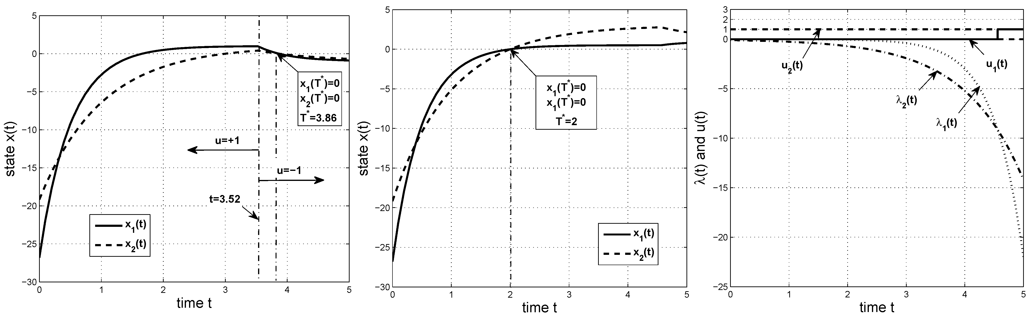
In this example, we treat $u_2$ as a redundant input channel. Initially, by applying Pontryagin’s Maximum Principle (PMP) [20] to the time-optimal control problem of the system described by Equation (44), which lacks input redundancy, we determine that the optimal time is $T^{*}=3.86$. This is illustrated on the left side of Figure 5, where the optimal state $x^{*}\left(t\right)$ reaches the origin at $t=3.86$, specifically $x_1\left(3.86\right)=0$ and $x_2\left(3.86\right)=0$. Subsequently, for the system outlined in Equation (45), which incorporates input redundancy, we ascertain that its optimal time is $T_{\Theta }^{*}=2$. This is depicted in the center of Figure 5, where the optimal state $x_{\Theta }^{*}\left(t\right)$ reaches the origin at $t=2$, with $x_1\left(2\right)=0$ and $x_2\left(2\right)=0$. Additionally, the optimal control $u_{\Theta }^{*}\left(t\right)$ is displayed on the right side of Figure 5, where $u_{\Theta }^{*}\left(t\right)={[0,1]}^T$ represents a bang-bang control throughout the entire optimal time interval $t\in [0,2]$.

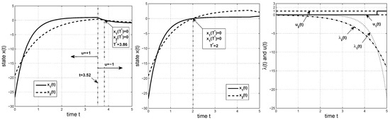
Figure 5. Time-optimal control of Example 1. Left: Dynamics of the optimal states $x^{*}\left(t\right)$ for Equation (44) without input redundancy, where $x^{*}\left(t\right)={[x_1\left(t\right),x_2\left(t\right)]}^T$. Center: Dynamics of the optimal states $x_{\Theta }^{*}\left(t\right)$ for Equation (45) with input redundancy, where $x_{\Theta }^{*}\left(t\right)={[x_1\left(t\right),x_2\left(t\right)]}^T$. Right: Dynamics of the costate vector $\lambda \left(t\right)$ and the optimal control $u_{\Theta }^{*}\left(t\right)$ for Equation (45) with input redundancy, where $\lambda \left(t\right)={[{\lambda }_1\left(t\right),{\lambda }_2\left(t\right)]}^T$, $u_{\Theta }^{*}\left(t\right)={[u_1\left(t\right),u_2\left(t\right)]}^T$.

Evidently, in accordance with Definition 2, the bang-bang control $u_{\Theta }^{*}\left(t\right)={[0,1]}^T$ signifies that the redundant input channel $u_2$ is a non-idle channel with respect to the initial state $x\left(0\right)={[-26.7991,-19.1673]}^T$. Consequently, based on our theoretical findings in Theorem 1, we expect the optimal time to satisfy $T^{*}>T_{\Theta }^{*}$, which is corroborated by the experimental outcomes, yielding $T^{*}=3.86$ and $T_{\Theta }^{*}=2$.

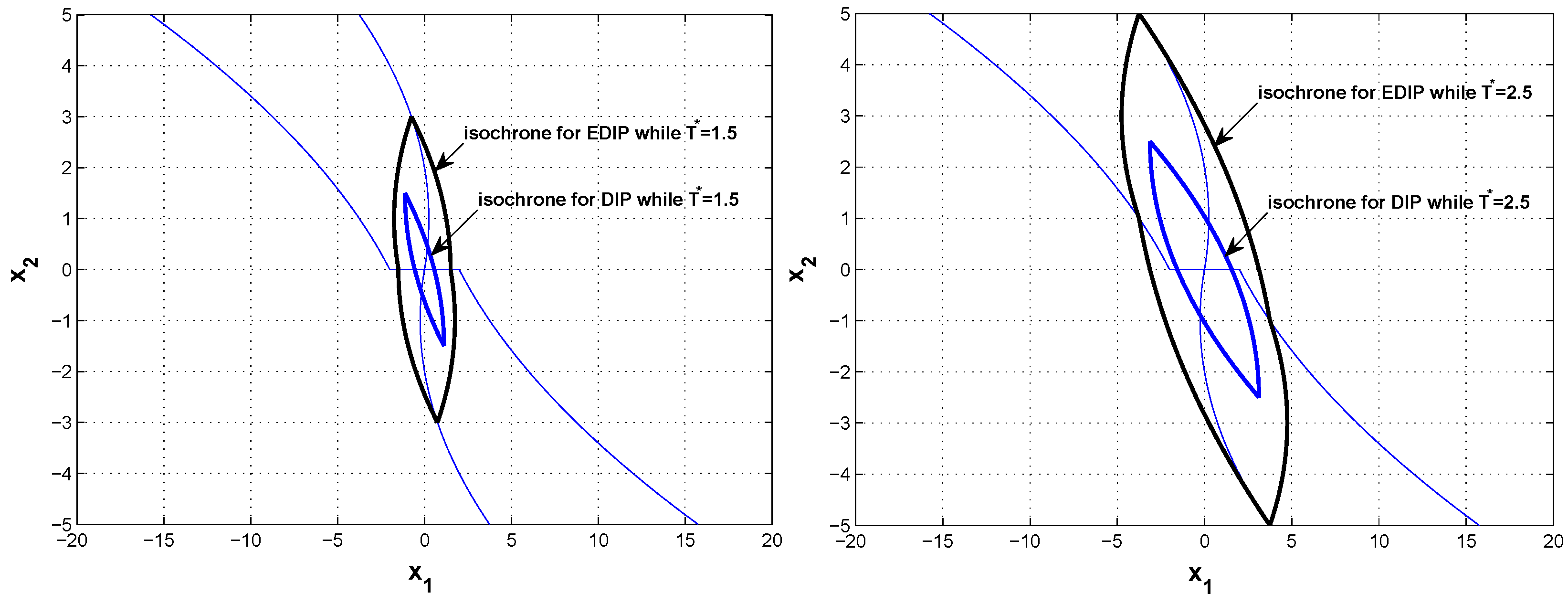
Example 2.

Compare with the time-optimal control problems of the double-integrator plant (DIP) [25] and the extended double-integrator plant (EDIP) to the origin point. The DIP is defined as

$$\begin{array}{c}\hfill \left[\begin{array}{c}{\dot{x}}_1\\ {\dot{x}}_2\end{array}\right]=\left[\begin{array}{cc}0& 1\\ 0& 0\end{array}\right]\left[\begin{array}{c}{x}_1\\ x_2\end{array}\right]+\left[\begin{array}{c}0\\ 1\end{array}\right]u_1,\end{array}$$

(47)

with the input constraint $|u_1|⩽1$. Meanwhile, the EDIP is defined as

$$\begin{array}{c}\hfill \left[\begin{array}{c}{\dot{x}}_1\\ {\dot{x}}_2\end{array}\right]=\left[\begin{array}{cc}0& 1\\ 0& 0\end{array}\right]\left[\begin{array}{c}{x}_1\\ x_2\end{array}\right]+\left[\begin{array}{cc}0& 1\\ 1& 1\end{array}\right]\left[\begin{array}{c}{u}_1\\ u_2\end{array}\right],\end{array}$$

(48)

with the following nondegenerate input constraint:

$$\begin{array}{c}\hfill u\left(t\right)=\left[\begin{array}{c}{u}_1\\ u_2\end{array}\right]\in {\Pi }_2=\left\{u\left(t\right):[0,+\infty )\to {\mathbb{R}}^{d\left(u\right)}|\left|u_i\left(t\right)\right|⩽1\mathrm{for}i=1,2\right\}.\end{array}$$

(49)

Undoubtedly, the time-optimal control problems associated with the systems described by Equations (47) and (48) in this example fulfill the criteria stipulated in Problems 5 and 6, respectively. It is evident that the linear time-invariant (LTI) systems expressed by Equations (47) and (48) are controllable. As a result, in line with Theorem 5, we can assert that

$$\begin{array}{c}\hfill T_{DIP}^{*}>T_{EDIP}^{*},\end{array}$$

(50)

holds true for any nonzero initial state.

Furthermore, we can leverage numerical experiments to substantiate the theoretical findings outlined in Equation (50). By applying PMP to this example, we depict the isochrones for the DIP and EDIP with optimal times of $T^{*}=1.5$ and $T^{*}=2.5$ in Figure 6. The isochrone corresponding to the DIP with $T^{*}=1.5$ delineates all initial states from which the system requires precisely $1.5$ s to reach the origin. Upon examining Figure 6, it is evident that the isochrone for the EDIP strictly encompasses that of the DIP for both $T^{*}=1.5$ and $T^{*}=2.5$. This observation indicates that the DIP invariably demands more time than the EDIP to transport the system from an identical initial state to the origin, thereby confirming our theoretical assertion in Equation (50).

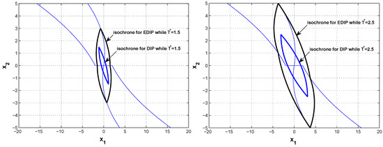
Figure 6. Isochrones of time-optimal control for Example 2. Left: Isochrones of $T^{*}=1.5$ for the DIP and EDIP. Right: Isochrones of $T^{*}=2.5$ for the DIP and EDIP.

4. Discussion

This paper introduces the notion of non-idle channels to ascertain the impact of input redundancy in time-optimal control problems. Within affine nonlinear systems, the presence of non-idle redundant channels ensures a strict decrease in the optimal time when input redundancy is incorporated. Provided that the input constraint is nondegenerate, the normality of the problem guarantees the existence of such non-idle channels. However, this assertion does not hold universally for degenerate input constraints. Contrary to typical expectations, duplicating the input channel may not lead to a reduction in the optimal time if the input constraint is of the form ${\Theta }_{d\left(u\right)}$. In linear time-invariant (LTI) systems, a controllable redundant input channel transforms into a non-idle channel, thereby reducing the optimal time.

Future research efforts might concentrate on extending the theoretical results to ensure a reduction in the optimal time for general nonlinear systems. Within affine nonlinear systems, identifying simpler conditions that guarantee the existence of non-idle redundant channels holds significant promise. Furthermore, it would be beneficial to explore the implications of adding input redundancy in the context of degenerate input constraints.

References

- Ikeda, Y.; Hood, M. An Application of L1 Optimization to Control Allocation. In Proceedings of the AIAA Guidance, Navigation and Control Conference and Exhibit, Denver, CO, USA, 14–17 August 2000. [Google Scholar]
- Shertzer, R.H.; Zimpfer, D.J.; Brown, P.D. Control allocation for the next generation of entry vehicles. In Proceedings of the AIAA Guidance, Navigation, and Control Conference and Exhibit, Monterey, CA, USA, 5–8 August 2002. [Google Scholar]
- Servidia, P.; Pena, R. Spacecraft Thruster Control Allocation Problems. IEEE Trans. Autom. Control 2005, 50, 245–249. [Google Scholar] [CrossRef]
- Sørdalen, O.J. Optimal thrust allocation for marine vessels. Control Eng. Pract. 1997, 5, 1223–1231. [Google Scholar] [CrossRef]
- Fossen, T.; Johansen, T. A Survey of Control Allocation Methods for Ships and Underwater Vehicles. In Proceedings of the 14th Mediterranean Conference on Control and Automation, Ancona, Italy, 28–30 June 2006. [Google Scholar]
- Spjøtvold, J.; Johansen, T. Fault Tolerant Control Allocation for a Thruster-Controlled Floating Platform Using Parametric Programming. In Proceedings of the IEEE Conference on Decision and Control and 28th Chinese Control Conference, Shanghai, China, 16–18 December 2009. [Google Scholar]
- Plumlee, J.; Bevly, D.; Hodel, A. Control of a Ground Vehicle Using Quadratic Programming Based Control Allocation Techniques. In Proceedings of the 2004 American Control Conference, Boston, MA, USA, 30 June–2 July 2004. [Google Scholar]
- Schofield, B.; Hagglund, T.; Rantzer, A. Vehicle Dynamics Control and Controller Allocation for Rollover Prevention. In Proceedings of the 2006 IEEE International Conference on Control Applications, Munich, Germany, 4–6 October 2006. [Google Scholar]
- Loria, C.; Kelly, M.; Hatney, R. X-31A quasi-tailless evaluation. In Proceedings of the 1996 IEEE Conference on Aerospace Applications, Aspen, CO, USA, 10 February 1996. [Google Scholar]
- Duan, Z.; Huang, L.; Yang, Y. The Effects of Redundant Control Inputs in Optimal Control. Sci. China Ser. F 2009, 52, 1973–1981. [Google Scholar] [CrossRef]
- Peng, Z.; Yang, Y.; Huang, L. The Effects of Adding Input Redundancies in Linear Quadratic Regulator Problems. J. Optim. Theory Appl. 2011, 150, 341–359. [Google Scholar] [CrossRef]
- Peng, Z.; Yang, Y. Evaluation of Input Redundancies on Linear Quadratic Regulator Problems. J. Optim. Theory Appl. 2012, 155, 325–335. [Google Scholar] [CrossRef]
- Liu, J.; Wang, L. New solution bounds of the continuous algebraic Riccati equation and their applications in redundant control input systems. Sci. China Inf. Sci. 2019, 62, 202201. [Google Scholar] [CrossRef]
- Liu, J.; Wang, L.; Bai, Y. New estimates of upper bounds for the solutions of the continuous algebraic Riccati equation and the redundant control inputs problems. Automatica 2020, 116, 108936. [Google Scholar] [CrossRef]
- Wang, L.; Zhou, L.; Zhang, L. The new solution bounds of the discrete algebraic Riccati equation and their applications in redundant control inputs systems. Asian J. Control 2023, 25, 4134–4144. [Google Scholar] [CrossRef]
- Liu, J.; Tang, F. A unified study of the redundant control input problem with different conditions in the stabilizable case. Int. J. Control 2024, 0, 1–16. [Google Scholar] [CrossRef]
- Jianzhou Liu, F.T.; Quan, H. High-performance LQR control for continuous time systems with redundant control inputs. Int. J. Syst. Sci. 2024, 55, 909–925. [Google Scholar] [CrossRef]
- Peng, Z.; Yang, Y.; Huang, L. Effects of Input Redundancy on Time Optimal Control. Acta Autom. Sin. 2011, 37, 222–227. [Google Scholar] [CrossRef]
- Electric Multiple Unit. Available online: http://en.wikipedia.org/wiki/Electric_multiple_unit (accessed on 1 April 2023).
- Pontryagin, L.; Boltyanskii, V.; Gamkrelidze, R.; Mishchenko, E. The Mathematical Theory of Optimal Processes; Wiley (Interscience): New York, NY, USA, 1962. [Google Scholar]
- Peng, Z.; Yang, Y.; Huang, L. Control Elimination of Time Optimal Bang-Bang Control with a Class of Input Constraints. In Proceedings of the 8th IEEE International Conference on Control and Automation, Xiamen, China, 9–11 June 2010. [Google Scholar]
- Athans, M.; Falb, P.L. Optimal Control: An Introduction to the Theory and Its Applications; McGraw-Hill, Inc.: New York, NY, USA, 1966. [Google Scholar]
- Chen, C.T. Linear System Theory and Design, 3rd ed.; Oxford University Press: New York, NY, USA, 1999. [Google Scholar]
- Rudin, W. Functional Analysis, 2nd ed.; McGraw-Hill: New York, NY, USA, 1991. [Google Scholar]
- Franklin, G.F.; Powell, J.D.; Emami-Naeini, A. Feedback Control of Dynamic Systems, 8th ed.; Pearson: London, UK, 2018. [Google Scholar]
Disclaimer/Publisher’s Note: The statements, opinions and data contained in all publications are solely those of the individual author(s) and contributor(s) and not of MDPI and/or the editor(s). MDPI and/or the editor(s) disclaim responsibility for any injury to people or property resulting from any ideas, methods, instructions or products referred to in the content. |
© 2024 by the authors. Licensee MDPI, Basel, Switzerland. This article is an open access article distributed under the terms and conditions of the Creative Commons Attribution (CC BY) license (https://creativecommons.org/licenses/by/4.0/).