Abstract
Indoor positioning is the key enabling technology for many location-aware applications. As GPS does not work indoors, various solutions are proposed for navigating devices. Among these solutions, Bluetooth low energy (BLE) technology has gained significant attention due to its affordability, low power consumption, and rapid data transmission capabilities, making it highly suitable for indoor positioning. Received signal strength (RSS)-based positioning has been studied intensively for a long time. However, the accuracy of RSS-based positioning can fluctuate due to signal attenuation and environmental factors like crowd density. Angle of arrival (AoA)-based positioning uses angle measurement technology for location devices and can achieve higher precision, but the accuracy may also be affected by radio reflections, diffractions, etc. In this study, a dual-branch convolutional neural network (CNN)-based BLE indoor positioning algorithm integrating RSS and AoA is proposed, which exploits both RSS and AoA to estimate the position of a target. Given the absence of publicly available datasets, we generated our own dataset for this study. Data were collected from each receiver in three different directions, resulting in a total of 2675 records, which included both RSS and AoA measurements. Of these, 1295 records were designated for training purposes. Subsequently, we evaluated our algorithm using the remaining 1380 unseen test records. Our RSS and AoA fusion algorithm yielded a sub-meter accuracy of 0.79 m, which was significantly better than the 1.06 m and 1.67 m obtained when using only the RSS or the AoA method. Compared with the RSS-only and AoA-only solutions, the accuracy was improved by 25.47% and 52.69%, respectively. These results are even close to the latest commercial proprietary system, which represents the state-of-the-art indoor positioning technology.
Keywords:
bluetooth low energy; indoor positioning; received signal strength; angle of arrival; convolutional neural network MSC:
68T07
1. Introduction
Localization-based services (LBSs) have witnessed increasing demand for both indoor and outdoor positioning systems. While outdoor technologies like GPS offer mature solutions for car navigation and hiking, indoor environments present distinct challenges due to signal attenuation and multipath effects caused by building structures. These limitations necessitate the exploration of alternative technologies for precise indoor localization. Ongoing research aims to further refine these techniques to meet the increasing demand for accurate indoor location services across various applications, from navigation assistance for the visually impaired to efficient asset management in commercial settings.
Radio frequency (RF) technologies have emerged as promising solutions for indoor positioning. In our previous work, technologies such as Wi-Fi, Bluetooth, radio frequency identification (RFID), ZigBee, and ultra-wideband (UWB) have been extensively investigated due to their AP applicability, low power consumption, and affordability. Among those technologies, BLE has evolved as a robust solution for indoor positioning, addressing challenges such as dynamic obstacles and fluctuating signal conditions. BLE stands out for its widespread adoption in Internet of Things (IoT) applications, particularly in indoor settings where it supports continuous monitoring of mobile users.
BLE-based indoor positioning systems represent a robust solution for addressing the challenges of indoor localization, offering scalability and efficiency across diverse applications from smart buildings to healthcare. Future developments will likely focus on refining existing algorithms, enhancing system robustness, and expanding application domains to further capitalize on the potential of BLE technology in indoor positioning. BLE technology has gained significant attention due to its affordability, low power consumption, and rapid data transmission capabilities, making it highly suitable for indoor positioning. BLE beacons, small wireless sensors that emit continuous radio signals, facilitate indoor localization by leveraging RSS measurements.
RSS-based methods leverage various methods including trilateration, triangulation, and fingerprinting. RSS-based methods estimate position by measuring signal strength but are susceptible to multipath interference and signal instability. Fingerprinting, a common technique within RSS-based systems, involves creating a database of signal fingerprints at known locations to match and estimate positions during real-time applications. Despite its simplicity, fingerprinting requires extensive initial data collection and computing resources for accurate positioning.
The introduction of Bluetooth 5.1 in 2019 has introduced direction-finding capabilities and promising centimeter-level precision, which has been evaluated using specialized equipment. AoA estimation involves determining incident RF wave directions using antenna arrays, enhancing accuracy through advanced signal processing techniques like Gaussian frequency shift keying (GFSK). Integrating deep learning with AoA and RSS measurements shows potential for further enhancing localization performance by mitigating signal quality issues, especially over greater distances where slight angular errors can significantly affect the positioning precision.
Research efforts have explored various algorithms and techniques to improve BLE-based indoor localization. These include machine learning models for fingerprint matching, nonlinear estimation algorithms for AoA, and hybrid approaches combining RSS and AoA to overcome limitations in individual measurements. Despite these advancements, challenges such as multipath effects, noise interference, and system complexity remain critical areas for ongoing research.
Despite these advancements, the accuracy of RSS-based positioning can fluctuate due to signal attenuation and environmental factors like crowd density. Research focuses on improving algorithms and filters to enhance positioning accuracy to approximately 2 m.
In addition to the RSS-based method, triangulations such as time of arrival (ToA), time of flight (ToF), time difference of arrival (TDoA), AoA, and angle of departure (AoD) are explored for indoor localization. These methods rely on specialized hardware to measure the signal time and angle, contributing to improved accuracy. In summary, the convergence of diverse wireless technologies and advanced positioning techniques continues to drive progress in the field, offering enhanced performance and expanding the scope of applications.
Despite significant progress in BLE-based indoor positioning systems, challenges related to accuracy, robustness, and adaptability to dynamic environments persist. This study aims to address these challenges by proposing a novel deep learning-based algorithm that integrates RSS and AoA features to enhance indoor localization.
While the existing literature shows increasing interest in BLE for indoor positioning, there is a notable gap in effectively fusing RSS and AoA measurements to improve accuracy under varying conditions. Previous research has primarily concentrated on optimizing either RSS-based algorithms or AoA measurements in isolation, often neglecting the potential benefits of their combined use. Moreover, many methods have struggled with issues related to environmental variability, sensor limitations, and the computational demands of deploying models in real-world scenarios.
This study addresses these gaps by developing a dual-branch deep learning model that combines the strengths of both RSS and AoA measurements. The focus is on enhancing the model’s robustness to environmental changes and sensor inaccuracies, thus offering a more reliable indoor positioning solution. The research introduces innovative techniques in feature fusion through a CNN, alongside advanced preprocessing methods like principal component analysis (PCA) and Kalman filtering. This approach aims to improve both the accuracy and adaptability of BLE-based indoor positioning systems, making them more effective and scalable for diverse and dynamic environments.
The main contributions of this study are reported below:
- Real-world measurement-based AoA and RSS dataset: Given the absence of publicly available datasets, we generated our own dataset for this study. The dataset included Bluetooth 5.1 AoA and RSS values from the LAUNCHXL-CC2640R2 development kit manufactured by Texas Instruments (TI). The data were collected from each receiver in three different directions, resulting in a total of 2675 records, which included both RSS and AoA measurements. Of these, 1295 records were designated for training purposes, while the remaining 1380 were unseen test records. The dataset allowed the reproduction of indoor positioning and detection algorithms at realistic conditions.
- Enhanced indoor positioning model: We introduced a novel indoor positioning model that used a dual-branch CNN, optimized for processing the spatial dependencies in both AoA and RSS data transformed into image-like formats. This model addressed the shortcomings of traditional single RSS or AoA fingerprinting methods by effectively handling the environmental dynamics within indoor settings. The advantage of considering both was that they were affected in different ways by varying impediments in the radio environment, and the initial results presented in this study showed that combining the techniques offered (i) the ability to achieve greater accuracy and (ii) the potential of using machine learning to enhance the accuracy as the environment changes.
- Experimental validation: Experiments were conducted on our dataset. The effectiveness of the proposed model and algorithms was validated through rigorous field tests within a meticulously prepared indoor environment. This included the collection of a significant dataset that captured the complexity of real-world conditions. The performance of the experimental validation demonstrates expected results.
The structure of this paper is the following: Section 2 presents an overview of applicable research; Section 3 outlines the methodology employed for indoor positioning and explains the designs of positioning algorithm; and Section 4 encompasses the construction of the experimental site, thorough data analysis, rigorous evaluation of algorithms, and resolution of existing questions. Finally, in Section 5, we summarize the findings of our research, spotlighting achievements and limitations, and propose prospective research directions.
2. Related Works
2.1. Wireless Positioning Technologies
Wireless positioning technologies have seen significant advancements in recent years, aiming to enhance accuracy and efficiency for both indoor and outdoor localization. These technologies include a variety of methods such as sensor fusion, simultaneous localization and mapping (SLAM), pedestrian dead reckoning (PDR), and integrated sensing, which leverage wireless communication and sophisticated sensors to improve positioning systems [1]. The emergence of technologies like 5G and UWB has further refined wireless positioning, enabling sub-meter precision and opening up new application areas like IoT, self-driving cars, and contact tracing [2]. Additionally, the utilization of widely deployed Wi-Fi equipment in conjunction with deep learning methods has led to high-precision indoor positioning, ensuring long-term accuracy while reducing maintenance costs [3].
ToA, ToF, and ToDA are crucial technologies in indoor positioning systems. Additionally, a proposed UWB indoor positioning system utilizes ToF ranging and a weighted centroid algorithm for initial tag position estimation, enhancing positioning reliability under varying noise conditions [4]. Moreover, a method for measuring the ToF and ToDA in indoor positioning systems has been developed, emphasizing fast positioning speed, low cost, and high precision, particularly suitable for wireless network equipment positioning indoors [5]. Experimental comparisons have demonstrated that a ToF–direction of arrival (DoA) hybrid method can significantly reduce positioning errors compared with ToF-only methods, showcasing the potential for accurate indoor positioning with compact array antennas at anchor stations [6]. ToA and DoA estimation for indoor positioning with 5G pico-cell base stations is addressed in the paper, focusing on efficient joint estimation [7].
2.2. RSS-Based Indoor Positioning Methods
RSS-based indoor positioning systems are widely used due to the prevalence of Wi-Fi access points indoors [8]. However, the performance of traditional RSS-based methods is hindered by the complex and dynamic indoor environments. To address this limitation, innovative approaches have been proposed. Liang, Yuan, et al. utilized RSS distribution from passive radio frequency (PRF) signals for three-dimensional positioning [9]. Guangyi, Guo et al. developed collaborative indoor positioning methods leveraging neighboring devices as additional anchors to enhance accuracy through multilayer perceptron (MLP) neural networks. These advancements aim to improve the accuracy and robustness of indoor positioning systems, offering better performance compared with conventional methods, with reported average positioning accuracies as low as 0.572 m [10].
Gao, Ren, et al. evaluate five filtering methods (limit, threshold, max, MA, and Kalman) for improving indoor positioning accuracy based on RSS in wireless LANs, with limit and threshold filters showing significant enhancement [11]. Sangwoo, Lee, et al. employed a Kalman filter integrating with self-calibration to mitigate RSS variation in indoor position tracking, enhancing accuracy by mapping offline and online RSS measurements [12].
Ossi, Kaltiokallio, et al. introduce a novel Bayesian filter for RSS-based device-free localization and tracking, combining imaging and Bayesian approaches for robustness and accuracy in position estimation [13].
Zhenghuan, Wang et al. utilized a particle filter for tracking in RSS-based device-free localization (DFL) systems. It provides an approximate Bayesian estimate of target position, enhancing tracking accuracy in DFL applications [14]. Jing-Huei et al. proposed a dataset offering dense and uniformly distributed reference points (RPs) for Wi-Fi indoor localization, with an average distance between RPs smaller than 1.2 m, facilitating high-precision positioning and fine-grained scene identification [15].
2.3. AoA-Based Indoor Positioning Methods
AoA technology plays a crucial role in indoor positioning systems, offering the potential for high accuracy in localization. Research has shown that AoA of Wi-Fi and Bluetooth signals can achieve decimeter-level accuracy benefiting from recent innovations. Xianan, Zhang et al. proposed an AutoLoc, a system that eliminates uncertain initial phases for precise AoA estimation without the need for manual calibrations or extra sensors [16]. Bluetooth 5.1 introduces direction-finding capabilities that enable the localization of objects or individuals in indoor environments, enhancing the development of intelligent navigation systems for hospitals and other facilities [17]. By leveraging AoA techniques and multiple anchor receivers, indoor localization systems can significantly improve wayfinding efficiency, reduce operational burdens, enhance patient experiences, and elevate the digital management standards of various establishments [18]. Hyukwoo, Lee et al. suggested using AoA measurements for localization, with a Kalman filter-based hypothesis test to identify non-line-of-sight (NLoS) noise and a real-time localization system (RLS) scheme for precise target location estimation [19].
2.4. RSS and AoA Fusion Methods
D. Zhu et al. proposed a deep learning indoor localization algorithm base on a Bluetooth RSS and AoA dataset in a classroom from TI evaluation boards [20]. D. Sun et al. collected Bluetooth RSS and AoA data for indoor localization in a wide open room located in their research institute in Italy [21].
Indoor positioning systems often face challenges due to signal reflections and uncertainties, leading researchers to explore fusion methods combining the RSS and AoA for enhanced accuracy. Various studies propose innovative approaches to address these challenges. Wang et al. introduce a fusion positioning method utilizing acoustic signals and inertial measurement unit (IMU) data, demonstrating stable positioning even with unilateral data loss [22]. Kim et al. present a method combining RSS and AoA in a single light emitting diode (LED) transmitter and multiple sensor receiver setups, showcasing improved indoor positioning accuracy [23]. Zhang et al. propose a weighted least square method combining RSS and AoA measurements to reduce positioning deviations in indoor environments [24]. Zaal et al. discuss the advantages of hybrid algorithms, particularly the AoA/RSS fusion with Omni and directional antennas, highlighting increased accuracy in indoor localization [25]. Ding et al. introduce a hybrid RSS/AoA method based on error variance and measurement noise weighted least squares, achieving high-precision indoor positioning without complexity [26]. These studies collectively emphasize the effectiveness of RSS and AoA fusion techniques in enhancing indoor positioning accuracy. Tomic et al. studied the problem of target localization based on combining RSS and AoA measurements from a geometrical perspective. Their solution matches the localization accuracy of existing methods and outperforms them considerably when the number of reference points is low [27]. Wang et al. addressed an indoor target tracking system based on combined measurements of RSS and AoA, which targets the nonlinear state estimation of the system and the multi-sensor fusion problem considering the correlation of local estimation errors. They proposed a high-order modified extended Kalman particle filter (HM-EKPF) with improved proposal distribution, and experimental results demonstrate that the tracking accuracy of the proposed HM-EKPF method is improved by 10.8%, and the average tracking error after fusion is reduced by 12.2% compared with existing methods [28]. Wang et al. examine source localization utilizing AoA and a hybrid approach combining RSS with AoA measurements. Their numerical simulations demonstrate that the proposed methods exhibit superior performance in both AoA and hybrid AoA/RSS localization scenarios. The accuracy of these methods is comparable to or exceeds that of the traditional least squares (LS) techniques reported in the literature [29].
Although the abovementioned studies have thoroughly reviewed RSS and AoA fusion methods, their results assume that the underlying models or parameters are known or can be accurately estimated. However, in practice, obtaining such carefully selected models or parameters can be challenging. Consequently, developing new methods that address cases where model parameters are unknown remains an open research question, which also includes the gaps in the existing studies.
3. Methodology
3.1. RSS and AoA Measurement and Data Acquisition
Bluetooth Standard 5.1 incorporates support for AoA measurements alongside RSS, significantly enhancing capabilities for achieving high-precision real-time positioning. AoA measurement functionality necessitates Bluetooth receivers equipped with antenna arrays, typically comprising at least three independent antennas. Each antenna within the array captures the phase of the received radio signals. Leveraging the known distances between antennas, the AoA of a Bluetooth signal can be accurately determined based on the observed phase differences.
For our investigation, we employed the LAUNCHXL-CC2640R2 development kit [30] manufactured by Texas Instruments™, chosen for its early availability and robust functionality. This development kit featured two integrated array antennas, each comprising three elements angled at 90°, facilitating the precise estimation of signal angles using the AoA method. The CC2640R2 board, along with the AoA antenna board, was positioned horizontally for optimal measurement.
During experimentation, a development toolkit equipped with directional antennas was mounted on tripods at each corner of an approximately rectangular experimental site. A separate toolkit equipped with an omnidirectional antenna served as a mobile transmitter, enabling flexible movement within the field to gather data, as illustrated in Figure 1.
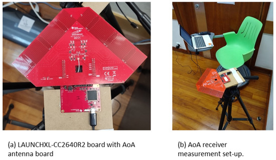
Figure 1.
Measurement of RSS and AoA.
Following the setup outlined in the official documentation, each receiver was configured to capture angle readings and transmit them to a computer via a network file transfer application. Extra-PuTTY version 0.30, a third-party software, was utilized to accurately timestamp log records in milliseconds, addressing logging time issues. Data logging occurred at each measurement point using receivers, generating log files formatted from PuTTY data outputs. Each log file recorded four attributes sequentially: the AoA, RSSI, antenna specifications, and channel information shown as Figure 2.
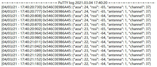
Figure 2.
Sample log output with timestamp.
In addition, Python scripts were utilized for various tasks including importing raw data into Excel, introducing random Gaussian noise to experimental results, and implementing Kalman filtering. The Kalman filter, a renowned algorithm for predicting and forecasting motion trajectories, was employed to refine the localization accuracy by filtering the data. Simultaneously, a Pauta criterion-based filter was incorporated within the algorithmic framework to detect and remove visibly erroneous data points.
3.2. RSS-Based Position Estimation Method
Based on the measurement distance, for each result, a circle was drawn from the corresponding receiver at the distance the receiver determined the signal to have come from, and the three nearest intersections of the three circles were found. The midpoints of each side of the arcs formed by the four intersections were connected, and the intersection of those connections was taken as the measure result. The green point is the actual position, while the red point is the estimated position. This is illustrated in Figure 3, which shows the positions from results. And the calculated processing is described by Algorithm 1.
| Algorithm 1 RSS-Based Position Estimation |
| 1: Input: : RSSI measured by receivers |
| 2: Output: : estimated position |
| 3: Start |
| 4: for each (, in {(, } do |
| 5: |
| 6: |
| 7: end |
| 8: |
| 9: |
| 10: |
| 11: )/3, )/3) |
| 12: End |
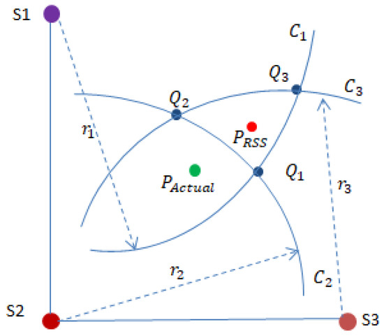
Figure 3.
Calculation of position from RSS measurements.
The error distance between the actual point and the measurement point is defined as Formula (1):
3.3. AoA-Based Position Estimation Method
Based on the measurement angle, for each result, a ray was drawn from the corresponding receiver at the angle at which the receiver determined the signal to have come from, and the four nearest intersections of the four rays were found. The midpoints of each side of the quadrilateral formed by the four intersections were connected and the intersection of those connections was taken as the measure result. Figure 4 depicts the spatial positions derived from the experimental outcomes. The actual position is represented by a green point, whereas the estimated position is denoted by a red point. Additionally, Algorithm 2 details the computational procedure employed for the calculations.
| Algorithm 2 AoA-Based Position Estimation |
| 1: Input: : angles measured by receivers |
| 2: Output: : estimated position |
| 3: Start |
| 4: for each (, in {(, } do |
| 5: |
| 6: end |
| 7: |
| 8: |
| 9: |
| 10: )/3, )/3) |
| 11: End |
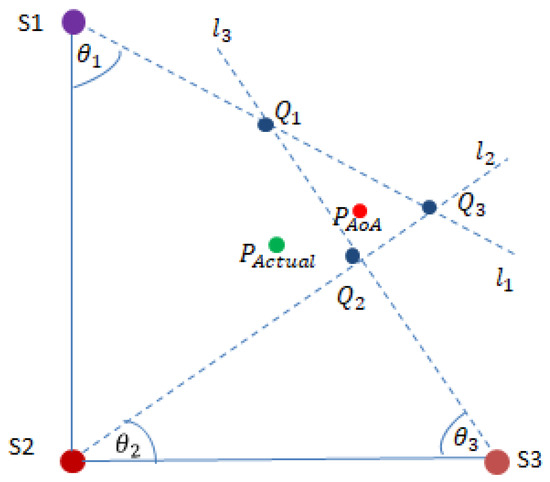
Figure 4.
Calculation of position from AoA measurements.
The error distance between the actual point and the measurement point is defines as Formula (2):
3.4. Theoretical Analysis of Fusing RSS and AoA
A significant challenge in Bluetooth positioning is managing the radio environment, where various objects may absorb or reflect the radio signals. An even more complex issue is the dynamic changes in these environmental factors. For example, in a large warehouse, there may be minimal line-of-path obstructions and limited dynamic changes; when guiding partially sighted individuals in urban environments that can become crowded at certain times, the changes in radio signal impairments can be significant. In our experience, even basic tests with commercial equipment illustrate the challenges of setting up a proper indoor positioning system, even in a relatively simple environment. The algorithms used in most commercial equipment are proprietary, but it is the authors’ understanding that both RSS and AoA are included.
Since the perceived RSS and AoA may be affected differently by these impairments, it is sensible to consider how they may be combined to provide more accurate positioning.
The work presented here was an investigation into such a combining as shown in Figure 5. The approach taken here to determine a test set of data that could be used for training was as follows:
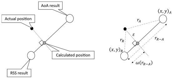
Figure 5.
Outline scheme for combining RSS and AoA.
- (i)
- For every test point, obtain pairs of location values for RSS and AoA: and respectively.
- (ii)
- Then, knowing the locations, it is straightforward trigonometry to determine the line normal to the line between and that passes through the actual location.
- (iii)
- The intersection of these two lines is the calculated position of the target.
- (iv)
- Calculate ω, the proportion of the distance between the RSS-found position and the AoA-found position, measured from the RSS end.
While it was clear that there was still most likely to be an error ε, the trigonometry showed that, provided the line through the actual position was normal, the error ε was less than that to either of the RSS and AoA found positions. This led us to investigate the performance of an AoA-based method and how to combine the results from RSS and AoA. Key to this approach is the mapping of the new data to the training set, and although this is shown by finding the nearest region, the best approach may be something different, like a neural network or other form of machine learning.
3.5. Dual-Branch CNN Architecture by Fusing RSS with AoA
The proposed algorithm encompassed distinct phases, namely, the offline phase and the online phase. During the offline phase, RSS and AoA measurements were acquired at various reference positions, yielding datasets denoted as DR = {R1; …; RM}, where Ri = {ri1; …; riN}, and DA = {A1; …; AM}, where Ai = {ai1; …; aiN}, N represents the number of samples in the dataset, and M represents the number of BLE beacons. DR denotes the RSS dataset, while DA represents the AoA dataset in our analysis. Subsequently, we used ordinary filtering based on the Pauta criterion as in Algorithm 3 and Kalman filtering as in the Algorithm 4 techniques for noise mitigation. Subsequent to these preprocessing steps, a CNN architecture was employed for feature extraction, followed by the utilization of a Soft-max layer for classification-based learning. Consequently, a localization classification model was formulated. In the subsequent online phase, data preprocessing procedures, coupled with feature extraction techniques, paved the way for the application of the classification model to yield the ultimate estimation of the positional coordinates.
| Algorithm 3 Pauta Criterion-Based Filter for AoA and RSS |
| 1: Input: |
| {, …, }, where = {; {,…,}, where = { |
| : number of samples of the dataset; : number of receivers |
| 2: Output: |
| {, …, }, where = {; {, …, }, where = { |
| 3: Start |
| 4: for do |
| 5: |
| 6: end |
| 7: for do |
| 8: for do |
| 9: if > + 3 * then = + 3 × end |
| 10: if < - 3 * then = - 3 × end |
| 11: if > + 3 * then = + 3 × end |
| 12: if < - 3 * then = - 3 × end |
| 13: end |
| 14: end |
| 15: End |
| Algorithm 4 Kalman Filter for AoA |
| 1: Input: |
| {, …, }, where = { |
| : number of samples of the dataset; : number of receivers |
| 2: Output: |
| {, …, }, where = { |
| 3: Start |
| 4: x_est = 0.0 # Initial state estimation |
| 5: P_est = 1.0 # Initial state estimation error covariance |
| 6: Q = 1 × 10⁻¹ # Uncertainty in the forecasting proces |
| 7: R = 0.1 # Uncertainty in the measurement process |
| 8: F = 1.0 # State transfer matrix F |
| 9: H = 1.0 # Measurement matrix H |
| 10: for do |
| 11: # Store the filtered estimate |
| 12: for do |
| 13: x_pred = F × x_est # Prediction steps |
| 14: P_pred = F × P_est × F + Q # update step |
| 15: K = P_pred × H/(H × P_pred × H + R) # Calculate the Kalman gain |
| 16: # Updating the status estimate |
| 17: x_est = x_pred + K × ( [t] − H × x_pred) |
| 18: P_est = (1 − K × H) × P_pred # Update error covariance |
| 19: # Store the filtered estimate |
| 20: end |
| 21: end |
| 22: End |
3.5.1. The Model of the Proposed CNN
Our CNN model comprised three main components: an input layer, hidden layers, and an output layer. The input layer was designed to receive and process data formatted according to predefined specifications. The hidden layers incorporated convolutional layers, activation layers, pooling layers, and fully connected layers. The output layer was responsible for grid identification and position estimation, utilizing the fusion estimation algorithm detailed in Section 3.5.3. The operation of each layer can be represented by the following formulas [31].
In the convolutional layers, the feature map was derived through the convolution of the RSS and AoA fingerprint data images. The convolution operation is described by Formula (3):
where A represents the feature map with coordinates (x, y). K denotes the convolution kernel, while P is the two-dimensional matrix of image pixel values input to the convolution operation. The coordinates (k, l) specify the position of the convolution kernel. The convolution process determines the distance between the positions of two adjacent scans as the convolution kernel traverses the feature map.
In the activation layers, the ReLU (rectified linear unit) function was utilized due to its computational efficiency, ability to address the vanishing gradient problem, and simplification of the calculation process, all of which aligned with the experimental requirements, which are given by Formula (4):
Given the output Z from the convolution layer, the ReLU activation function replaced all negative values in Z with zero, while positive values remained unchanged. This introduced non-linearity and helped the network learn more complex patterns.
The max pooling function was employed to reduce the dimensions of each feature map while preserving essential information. Let P denote the size of the pooling window (e.g., 2 × 2) and S represent the stride of the pooling operation. The output of the max pooling operation is described by Formula (5):
where and are the height and width of the pooling window. (x, y) denotes the position in the pooled feature map. The max pooling reduced the spatial dimensions of the feature map A by selecting the maximum value from each pooling window. This helped reduce computation and control overfitting by abstracting the feature representation.
In the fully connected layer, each neuron was connected to all neurons in the preceding layer through weighted connections. This operation was crucial for classifying the data or generating the final predictions. Let F represent the flattened input vector from the previous layer, W denote the weight matrix of size m × n (where m is the number of output neurons and n is the size of the flattened input vector), and b be the bias vector of size m. The output Y of the fully connected layer is described by Formula (6):
where is the output for neuron j, and is the ith element of the flattened input vector.
Based on this model and utilizing the characteristics of our experimental data and environment, we developed a convolutional neural network (CNN) for grid determination and location classification. All actual parameters used in Formulas (3)–(6) are listed in Table 1.

Table 1.
Parameters of the formulas.
3.5.2. Dual-Branch CNN Architecture
The CNN employs convolution as a specialized linear operation across one or multiple layers, distinct from conventional matrix multiplication. This architectural framework offers significant benefits for the analysis of data organized in grid-like structures, such as images or time series data. In this study, we changed the single-branch CNN model in our previous work [32] to a dual-branch architecture consisting of an RSS branch and an AoA branch. Moreover, we optimized its performance through parameter adjustments including filter dimensions, feature map configurations, and layer depth.
The experimental setup involved partitioning into uniform-sized blocks, where AoA and RSS measurements were systematically collected at specified training locations. Each location was typically detected by the receivers, capturing comprehensive measurements. The resulting dataset included labeled data points, with a subset allocated for training purposes and another subset reserved for testing. The original dataset comprised RSS and AoA measurements from deployed receivers along with corresponding spatial coordinates for each recording location.
To enable effective feature extraction using our CNN, we reformatted these data into a structure resembling an image. Specifically, the original testing area, previously partitioned into grids was expanded to form an M × N grid representation. Let I = max{M, N}. The parameters of our CNN architecture were set as follows: input layer, [I, I, 1] grayscale; two convolution layers, number of the filters [3, 3] and filter sizes [3, 2] with valid padding; two max-pooling layers, number of filters [8, 8] and filter sizes [2, 2]; one dense layer, 16 nodes; output layer, one representing x and y coordinates; and activation function, ReLU. Additionally, other hyperparameters, such as the batch size, number of layers, and layer sizes, could be modified during the testing procedure to facilitate the attainment of optimal positioning performance. Our CNN network architecture is illustrated in Figure 6.
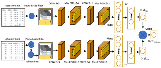
Figure 6.
Proposed CNN network architecture.
3.5.3. RSS and AoA Fusion Algorithm
The branch based on AoA was different from the branch based on RSS in data pre-processing. It included not only Pauta-based filtering but also Kalman filtering. The experimental results indicated that the RSS-based branch for prediction yielded smaller errors compared with AoA. Therefore, the prediction of served as a basis, and adjustments were performed by adding or subtracting the product of and . Thus, is defined as Formula (7):
where r is the distance between , and is the calibration parameter, which ranges in the interval (0, 1). In practice, there are four possible orientations between and similarly four between . These orientations are decomposed into horizontal and vertical components, as depicted in Figure 7 for observation. The correction algorithm for predicted and validated points based on RSS and AoA is presented as Algorithm 5.
| Algorithm 5 Correction Algorithm for RSS and AoA |
| 1: Input: : predicted coordinate by AoA-based CNN network; : predicted coordinate by RSS-based CNN network; : validate coordinate the scaling parameter |
| 2: Output: |
| : result coordinate |
| 3: Start 4: = abs (); # distance on axis x 6: 7: ; 8: else 9: ; 10: end 11: else 12: 13: ; 14: else 15: ; 16: end 17: end = abs (); #distance on axis y |
20: 21: ; 22: else 23: ; 24: end 25: else 26: 27: ; 28: else 29: ; 30: end 31: end |
| 32: End |
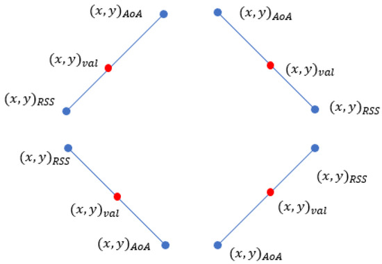
Figure 7.
Potential orientations of prediction points based on RSS and AoA.
4. Experiment and Results Analysis
4.1. Experimental Schematic
The experiments were conducted in Room N56A, Wui Chi Building, Macao Polytech-nic University, which spanned an area of 63 square meters (9 m × 7 m). The floor was characterized by tiles of 60 × 60 cm, giving rise to a regular grid in which we could easily annotate the location’s coordination. The term “grid” here refers to the actual coordinates and timestamps of the target being localized, such as a person moving along a defined path.
The room was furnished with desks and chairs, creating a realistic and complex indoor environment. Three receivers were deployed, and a transmitter was affixed to a movable tripod. The locations of the receivers were denoted by three blue dots labeled with letters representing their identifiers. Additionally, three red dots marked the start, end points, and inflection points of the paths traversed during the experiment, forming two straight-line segments.
During the experiment, the transmitter moved along straight paths from the “start” point to the “middle” point and then to the “end” point, as illustrated in Figure 8. The positions of the three receivers resulted in three measured rays forming a triangular area, with the geometric center of this triangle serving as the calculated position. The measurement process was repeated twice, with the data from the first set used as the training dataset and the data from the second set used as the test dataset.
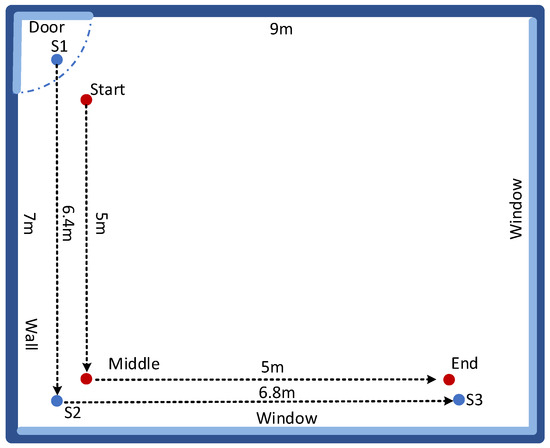
Figure 8.
Diagram of the experimental schematic.
4.2. Experimental Settings
4.2.1. Initial Format of Datasets
Each set of the development toolkit, a TI evaluation board, and the base tripod was combined together to form a receiver, with a total of three receivers placed at the three corners of the experimental area as reported in Figure 1. The experimental data were acquired using a receiver that was specifically configured to detect the signals of the sender. Each data record consisted of the AoA, RSSI, channel number, antenna number, and timestamps derived from the receiver as reported in Figure 2.
The experimental area was partitioned into a 0.6 m × 0.6 m grid; we analyzed the AoA and RSS collections, which were conducted at 17 training points, shown as blue grids. Three receivers typically detected each point, with all measurements captured. Figure 9 displays the arrangement of the receivers, training points, and testing points within the office setting. The 17 blue grids denote the training points, along the test motion path. For each training grid, 1295 records were collected in each of the three different directions. Meanwhile in each of the testing grids, 1380 records were gathered. Upon filtering out any invalid records, the total number of valid data points was found to be 2675 records.
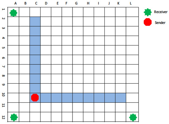
Figure 9.
Training and testing points setting.
To facilitate the use of CNNs for feature extraction, we have transformed these data into an image-like format. Our testing area, originally divided into grids labeled A–L and 1–12, was expanded to create a 12 × 12 grid representation, as illustrated in Figure 9.
The dataset was designed with AoA and RSSI readings from the sender and the coordinates of each recording point as presented in Figure 10. At each data collection point, multiple entries were recorded. For each data entry, the RSS and AoA values of the transmitter were recorded from three separate receivers. Additionally, the original row and column labels, ranging from “A” to “L” and “1” to “12”, were included. To simplify the location calculations, these coordinates were remapped to integer values ranging from 1 to 12, both horizontally and vertically. These coordinates were utilized for both training the model and subsequent positioning tasks.
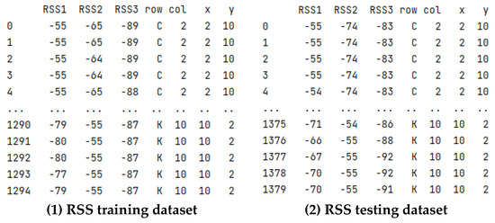
Figure 10.
Initial format of datasets.
The initial grid layout consisted of a 12 × 12 rectangular arrangement. In Figure 11, the left side illustrates this grid, where measurement values (RSS or AoA) from each receiver were positioned within their respective grid cells. For the right side, the RSS or AoA data were normalized to a real number between 0 and 1. For instance, the green dot located in grid C2 had coordinates of (2, 10) according to the RSS measurements, whereas the orange dot in grid K10 had coordinates of (10, 2) based on the AoA measurements.
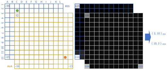
Figure 11.
Mapping original data into a grayscale image.
As for streamline processing with CNNs, the data were normalized using a straightforward formula (as shown in Formula (8)) to scale the RSS and AoA values to a real number between 0 and 1. In this scheme, 0 represents pure black, and 1 represents pure white, with intermediate values depicted in varying gray shades.
4.2.2. Data Preprocessing
The Pauta criterion-based filter discussed in Section 3.5.1 served to mitigate the inherent redundancy within the AoA and RSS measurements, while the Kalman filter algorithm in Section 3.5.2 was employed to temporally enhance the coherence of the AoA measurements. This preprocessing approach combined both filters, aiming to preserve relevant features while reducing noise and interference. This enhancement significantly improved the efficacy of localization performance. Given the importance of RSS and AoA data, maintaining the inherent dimensionality of information during subsequent network learning stages was crucial. Additionally, normalization procedures were applied to the RSS measurements to ensure consistent treatment across the dataset.
4.2.3. Feature Extraction Network Parameters
The proposed CNN network, configured with dual-branch inputs, was employed to extract relevant features from RSS measurements. The network architecture consisted of two convolutional layers followed by two max-pooling layers, concluding with a flatten layer. The convolutional operations were utilized to extract intricate features inherent in both AoA and RSS measurements. Subsequently, the max-pooling layers selectively preserved significant attributes while reducing data dimensionality. This approach contributed to parameter reduction and alleviated computational overheads, thereby mitigating overfitting risks. Detailed configuration parameters governing the feature extraction module are provided in Table 2. The input data, originally twelve-dimensional, underwent transformation, resulting in an RSS feature output of two-dimensional dimensionality.
Table 2.
Feature extraction network parameters.
4.2.4. Position Classification Learning Network Parameters
The network architecture parameters designed for classification learning were comprehensively detailed in Table 3. These parameters included a pair of fully connected layers followed by a Softmax layer, which functioned as the classifier. The RSS and AoA feature vectors were individually processed through the fully connected layers, culminating in the Softmax layer to produce classification outcomes. The rectified linear unit (ReLU) served as the chosen activation function for its effectiveness in enhancing the network’s ability to capture nonlinear relationships.
Table 3.
Classification learning network parameters.
For evaluating model performance, the mean squared error (MSE) was employed as the loss function, providing a quantitative measure of the disparity between the predicted and actual values. In terms of network optimization, the stochastic gradient descent (SGD) algorithm was utilized. Additionally, the network’s training regimen incorporated a polynomial learning strategy characterized by cyclic adjustments to the learning rate, facilitating adaptive convergence toward minimizing the global loss.
Based on extensive testing and accounting for the specific characteristics of the input data, optimal performance in our position classification task was consistently achieved when the batch size was set to 100, the learning rate was set to 0.001, and the training epoch was set to 1000.
4.3. Result Analysis
To assess the efficacy of our method, we defined the following formulas to compute the loss of our algorithms. Specifically, these formulas (designated as Formula (9), Formula (10), Formula (11), and Formula (12)) calculated the average distance error for each predicted coordinate.
To compare the values of and , we introduce δ, to compare the loss between the RSS and AoA-based and the RSS-based method. A positive value indicated that the RSS and AoA-based method performed better than the RSS-based method.
As reported as Figure 5 discussed at Section 3.5, we set the values in the range of (0, 1), and the test results are presented in the Table 4.
Table 4.
Test results in range of ω.
The average loss values for the RSS-based, AoA-based, and RSS and AoA-based methods were 2.08, 3.68, and 2.02, respectively. When converted to average distance errors by multiplying with 0.6, these values corresponded to 1.25 m, 2.2 m, and 1.21 m. Across all instances, the loss for RSS remained consistently lower than that for AoA, suggesting a preference for weighting the RSS component more heavily in the RSS and AoA-based fusion algorithm.
The lowest loss value observed was 1.32 for the RSS and AoA-based method at ω = 0.1, corresponding to an error distance of 0.79 m, calculated from 1.32 multiplied by 0.6. In comparison, the losses for the RSS-based and AoA-based methods were 1.76 and 2.78, resulting in error distances of 1.06 m and 1.67 m, respectively.
The value of δ indicated that when ω was 0.6 or less, the loss for the RSS and AoA-based method was smaller than that for RSS; conversely, it became larger when ω exceeded 0.6. A negative δ suggested that as ω decreased below 0.6, the gap in loss between the two methods widened, indicating improved performance for the RSS and AoA-based method. At ω = 0.5, the discrepancy between the two was nearly zero, suggesting minimal improvement.
However, as ω exceeded 0.6, δ became positive, indicating a decline in performance. The AoA-based method exhibited higher errors compared with the RSS-based method, yet integrating RSS and AoA could yield a smaller loss than using them separately. Overall, the observations suggested that smaller values of ω were preferable.
It is important to note that when ω = 0, the loss for the RSS and AoA-based method equaled that of RSS as only the RSS feature was considered, while AoA was excluded. Conversely, when ω = 1, the loss for the RSS and AoA-based method approached that of AoA alone since only the AoA feature was utilized, while RSS was not included. These extreme settings were not optimal for calculation and were typically not considered in the algorithm.
4.4. Comparison with Recent Works
We compared the performance of our proposed algorithm with our previous work [32]. Where the contrast algorithms were based on RSS or AoA, including K-nearest neighbor (KNN), weighted K-nearest neighbor (WKNN), naïve Bayes (NB), and an RSS-based neural network (RSS-NN) and RSS-CNN, all the comparative experiments were in a similar indoor experimental environment. The results of the comparison algorithms are presented in Table 5. The minimum error distance of our proposed algorithm was 0.79 m. Compared with the RSS-only and AoA-only solutions, the accuracy was improved by 25.47% and 52.69%, respectively.
Table 5.
Comparison of average distance error with recent works.
We investigated studies employing RSS and AoA fusion techniques such as references [28,29,31]; however, their experimental environments differed from ours. Moreover, these studies did not provide public datasets, which hindered direct and intuitive comparison. In future research, we will seek out studies that offer public datasets and facilitate more appropriate comparisons.
4.5. Discussion
Rather than treating the measurements individually, we combined them to study the problem from a geometrical perspective by exploiting the fact that the measurements were noise-corrupted. Our dual-branch CNN algorithm for Bluetooth indoor localization utilized the fusion of RSSI and AoA features. Feature extraction was conducted using a CNN, which separately extracted advanced features from both RSS and AoA data. These features were subsequently fused through a concatenation operation. For the final classification task, a Softmax layer was employed, leading to the development of the localization classification model. The proposed algorithm had significantly lower computational burden than the state-of-the-art approaches and not only matched their localization accuracy but also considerably outperformed them when the number of reference points was low.
Despite incorporating both RSS and AoA to enhance accuracy, the model was still vulnerable to environmental variations, such as crowd density, moving objects, and radio interference, which could impact measurement precision and overall performance. Implementing a dual-branch system with specialized CNN configurations and optimizing hyperparameters can be complex and resource intensive, potentially hindering the model’s adoption and replication across diverse environments. The model’s efficacy is heavily dependent on the quality and representativeness of the training data; insufficient data variety may impair the model’s generalizability in real-world settings. Additionally, dynamic changes in indoor environments require frequent recalibration to maintain accuracy, a process that can be laborious and impractical. The model’s performance is further constrained by the limitations of RSS and AoA sensors, including signal fluctuations and measurement precision issues.
Our research focused on addressing the problem of the guidance, with sufficient accuracy, of a visually impaired person in an indoor environment where the density of crowds varied. Examples of such locations are shopping centers, railway stations, and airports. The intention was to provide guidance through unfamiliar environments, to offer new opportunities to improve the quality of life of the visually impaired.
5. Conclusions
In this paper, we presented a comprehensive review of indoor positioning techniques utilizing RSS, AoA, and their fusion. We first studied a dual-branch CNN-based BLE indoor positioning algorithm integrating RSS and AoA, to explore how to enhance accuracy with combination techniques.
Two indoor experiments were conducted successfully, resulting in the acquisition of RSS and AoA datasets, which were subsequently divided into training and testing datasets. The experimental data underwent systematic analysis from various perspectives. Kalman filtering techniques were employed for noise mitigation in the AoA data. Additionally, the Pauta criterion-based filter was applied to pre-process the raw data for both RSS and AoA, resulting in noticeable improvements in accuracy. This approach was acknowledged as a stable and effective method overall.
In the course of our research, experiments were conducted to validate the performance of our proposed algorithms. The results demonstrated that RSS-based and RSS and AoA-based methods yielded average positioning distance errors of approximately 1.2 m. The algorithm achieved its highest accuracy of 0.79 m. Comparative analysis revealed that RSS alone outperformed AoA, while the combined approach of RSS and AoA exhibited superior performance in this experiment.
AoA-based methods may be better suited for compact environments with sparse reference points, whereas RSS methods may be more appropriate for larger spaces with numerous reference points. Integrating RSS and AoA can lead to reduced positioning error compared with using either method independently. In future research, we will explore the integration of other networks, including RNN, LSTM, and GRU, with the aim of further enhancing positioning accuracy.
Author Contributions
Investigation, X.Y.; writing—original draft, C.W.; writing—review & editing, Y.W.; supervision, W.K. All authors have read and agreed to the published version of the manuscript.
Funding
This work was funded by Macao Polytechnic University under grant number RP/FCA-03/2022.
Data Availability Statement
Data are contained within the article.
Conflicts of Interest
The authors declare no conflicts of interest.
References
- Isaia, C.; Michaelides, M.P. A Review of Wireless Positioning Techniques and Technologies: From Smart Sensors to 6G. Signals 2023, 4, 90–136. [Google Scholar] [CrossRef]
- Rydell, J.B.; Otterlind, O.; Sjöö, A. A Review of Wireless Positioning from Past and Current to Emerging Technologies. In Decision Support Systems and Industrial IoT in Smart Grid, Factories, and Cities; IGI Global: Hershey, PA, USA, 2021; pp. 39–41. [Google Scholar] [CrossRef]
- Zare, M.; Battulwar, R.; Seamons, J.; Sattarvand, J. Applications of Wireless Indoor Positioning Systems and Technologies in Underground Mining: A Review. Min. Met. Explor. 2021, 38, 2307–2322. [Google Scholar] [CrossRef]
- Nouali, I.Y.; Slimane, Z.; Abdelmalek, A. Change Point Detection-Based TOA Estimation in UWB Indoor Ranging Systems. In Proceedings of the 2022 45th International Conference on Telecommunications and Signal Processing (TSP), Prague, Czech Republic, 13–15 July 2022; pp. 329–332. [Google Scholar]
- Yang, J.; Zhu, C. Research on UWB Indoor Positioning System Based on TOF Combined Residual Weighting. Sensors 2023, 23, 1455. [Google Scholar] [CrossRef]
- Takahashi, Y.; Honma, N.; Sato, J.; Murakami, T.; Murata, K. Accuracy Comparison of Wireless Indoor Positioning Using Single Anchor: TOF only Versus TOF-DOA Hybrid Method. In Proceedings of the 2019 IEEE Asia-Pacific Microwave Conference (APMC), Singapore, 10–13 December 2019; pp. 1679–1681. [Google Scholar] [CrossRef]
- Pan, M.; Liu, P.; Liu, S.; Qi, W.; Huang, Y.; You, X.; Jia, X.; Li, X. Efficient Joint DOA and TOA Estimation for Indoor Positioning with 5G Picocell Base Stations. IEEE Trans. Instrum. Meas. 2022, 71, 1–19. [Google Scholar] [CrossRef]
- Yuan, L.; Chen, H.; Ewing, R.; Blasch, E.P.; Li, J. Three Dimensional Indoor Positioning Based on Passive Radio Frequency Signal Strength Distribution. IEEE Internet Things J. 2023, 10, 13933–13944. [Google Scholar] [CrossRef]
- Guo, G.; Chen, R.; Ye, F.; Liu, Z.; Xu, S.; Huang, L.; Li, Z.; Qian, L. A Robust Integration Platform of Wi-Fi RTT, RSS Signal, and MEMS-IMU for Locating Commercial Smartphone Indoors. IEEE Internet Things J. 2022, 9, 16322–16331. [Google Scholar] [CrossRef]
- Sun, X.; Zhuang, Y.; Huai, J.; Hua, L.; Chen, D.; Li, Y.; Cao, Y.; Chen, R. RSS-Based Visible Light Positioning Using Nonlinear Optimization. IEEE Internet Things J. 2022, 9, 14137–14150. [Google Scholar] [CrossRef]
- Gao, R.; Zhao, Y.; Tang, L. The Research on RSS Filter for Indoor Positioning System Based on Wireless LANs. Int. J. Adv. Inf. Sci. Serv. Sci. 2011, 3, 1–9. [Google Scholar] [CrossRef]
- Lee, S.; Cho, B.; Koo, B.; Ryu, S.; Choi, J.; Kim, S. Kalman Filter-Based Indoor Position Tracking with Self-Calibration for RSS Variation Mitigation. Int. J. Distrib. Sens. Netw. 2015, 11, 1–10. [Google Scholar] [CrossRef]
- Kaltiokallio, O.J.; Hostettler, R.; Patwari, N. A Novel Bayesian Filter for RSS-Based Device-Free Localization and Tracking. IEEE Trans. Mob. Comput. 2021, 20, 780–795. [Google Scholar] [CrossRef]
- Wang, Z.; Liu, H.; Xu, S.; Bu, X.; An, J. A Diffraction Measurement Model and Particle Filter Tracking Method for RSS-Based DFL. IEEE J. Sel. Areas Commun. 2015, 33, 2391–2403. [Google Scholar] [CrossRef]
- Bi, J.; Wang, Y.; Yu, B.; Cao, H.; Shi, T.; Huang, L. Supplementary open dataset for WiFi indoor localization based on received signal strength. Satell. Navig. 2022, 3, 25. [Google Scholar] [CrossRef]
- Yang, S.; Zhu, Y.; Gao, F.; Wen, C.; Huang, W. Research on Bluetooth AoA-based Indoor Navigation System for Hospitals. Highlights Sci. Eng. Technol. 2023, 39, 1394–1401. [Google Scholar] [CrossRef]
- Zhang, X.; Zhang, Y.; Liu, G.; Jiang, T. AutoLoc: Toward Ubiquitous AoA-Based Indoor Localization Using Commodity WiFi. IEEE Trans. Veh. Technol. 2023, 72, 8049–8060. [Google Scholar] [CrossRef]
- Furfari, F.; Barsocchi, P.; Girolami, M.; Mavilia, F. Modelling the Localization Error of an AoA-based Localization System. In Proceedings of the 2023 19th International Conference on Intelligent Environments (IE), Uniciti, Mauritius, 29–30 June 2023; pp. 1–4. [Google Scholar] [CrossRef]
- Lee, H.; Lee, K.; You, K. AOA Measurement based Localization Using RLS Algorithm under NLOS Environment. J. Phys. Conf. Ser. 2018, 1060, 012077. [Google Scholar] [CrossRef]
- Girolami, M.; Furfari, F.; Barsocchi, P.; Mavilia, F. A Bluetooth 5.1 Dataset Based on Angle of Arrival and RSS for Indoor Localization. IEEE Access 2023, 11, 81763–81776. [Google Scholar] [CrossRef]
- Zhu, D.; Yan, J. A Deep Learning Based Bluetooth Indoor Localization Algorithm by RSSI and AOA Feature Fusion. In Proceedings of the 2022 International Conference on Computer, Information and Telecommunication Systems (CITS), Piraeus, Greece, 13–15 July 2022; pp. 1–6. [Google Scholar] [CrossRef]
- Wang, H.; Wang, Z.; Zhang, L.; Luo, X.; Wang, X. A Highly Stable Fusion Positioning System of Smartphone under NLoS Acoustic Indoor Environment. ACM Trans. Internet Technol. 2023, 23, 1–19. [Google Scholar] [CrossRef]
- Kim, J.; Lim, J.; Baek, H. RSS/AOA Positioning Scheme Using Multiple Receivers in Indoor VLC Communications. J. Korean Inst. Commun. Inf. Sci. 2022, 47, 1322–1329. [Google Scholar] [CrossRef]
- Zhang, T.; Fu, J.; Wang, Y. RSS/AoA Indoor Target Location Method Based on Weighted Least Squares Algorithm. In Intelligent Equipment, Robots, and Vehicles; Springer: Singapore, 2021. [Google Scholar] [CrossRef]
- Zaal, R.M.; Abbas, E.I.; Mosleh, M.F. A Comprehensive Comparison for Different Hybrid Based Localization Algorithms for Indoor Communications. Eng. Technol. J. 2022, 40, 396–403. [Google Scholar] [CrossRef]
- Ding, W.; Chang, S.; Li, J. A Novel Weighted Localization Method in Wireless Sensor Networks Based on Hybrid RSS/AoA Measurements. IEEE Access 2021, 9, 150677–150685. [Google Scholar] [CrossRef]
- Tomic, S.; Beko, M. A New Perspective on Range and Directional Localization Problem. IEEE Open J. Veh. Technol. 2021, 2, 337–344. [Google Scholar] [CrossRef]
- Wang, Y.; Fu, J.; Wu, Z. A Novel Fusion Estimation Method for RSS-AOA-Based Indoor Target Tracking. IEEE Sens. J. 2024, 24, 22632–22647. [Google Scholar] [CrossRef]
- Wang, Q.; Duan, Z.; Li, X.R. Source Localization with AOA-Only and Hybrid RSS/AOA Measurements via Semidefinite Programming. In Proceedings of the 2020 IEEE 23rd International Conference on Information Fusion (FUSION), Rustenburg, South Africa, 6–9 July 2020; pp. 1–8. [Google Scholar] [CrossRef]
- LAUNCHXL-CC2640R2 Development Kit|TI.com. Available online: https://www.ti.com/tool/LAUNCHXL-CC2640R2#overview (accessed on 11 July 2024).
- Sun, D.; Wei, E.; Yang, L.; Xu, S. Improving Fingerprint Indoor Localization Using Convolutional Neural Networks. IEEE Access 2020, 8, 193396–193411. [Google Scholar] [CrossRef]
- Wu, C.; Wong, I.-C.; Wang, Y.; Ke, W.; Yang, X. Experimental Study of Bluetooth Indoor Positioning Using RSS and Deep Learning Algorithms. Mathematics 2024, 12, 1386. [Google Scholar] [CrossRef]
Disclaimer/Publisher’s Note: The statements, opinions and data contained in all publications are solely those of the individual author(s) and contributor(s) and not of MDPI and/or the editor(s). MDPI and/or the editor(s) disclaim responsibility for any injury to people or property resulting from any ideas, methods, instructions or products referred to in the content. |
© 2024 by the authors. Licensee MDPI, Basel, Switzerland. This article is an open access article distributed under the terms and conditions of the Creative Commons Attribution (CC BY) license (https://creativecommons.org/licenses/by/4.0/).