Modifications to the Jarque–Bera Test

Abstract

The Jarque–Bera test is commonly used in statistics and econometrics to test the hypothesis that sample elements adhere to a normal distribution with an unknown mean and variance. This paper proposes several modifications to this test, allowing for testing hypotheses that the considered sample comes from: a normal distribution with a known mean (variance unknown); a normal distribution with a known variance (mean unknown); a normal distribution with a known mean and variance. For given significance levels, $\alpha =0.05$ and $\alpha =0.01$, we compare the power of our normality test with the most well-known and popular tests using the Monte Carlo method: Kolmogorov–Smirnov (KS), Anderson–Darling (AD), Cramér–von Mises (CVM), Lilliefors (LF), and Shapiro–Wilk (SW) tests. Under the specific distributions, 1000 datasets were generated with the sample sizes $n=25,50,75,100,150,200,250,500,$ and 1000. The simulation study showed that the suggested tests often have the best power properties. Our study also has a methodological nature, providing detailed proofs accessible to undergraduate students in statistics and probability, unlike the works of Jarque and Bera.

1. Introduction

C. Jarque and A.K. Bera proposed the following goodness-of-fit test (see [1,2,3]) to determine whether the empirical skewness and kurtosis match those of a normal distribution. The hypothesis to be tested is as follows:

H₀. 

If the population the sample presents is normally distributed against the alternative hypothesis.

H₁. 

If the population the sample presents follows a distribution from the Pearson family that is not normally distributed.

More precisely, the null hypothesis is formulated as follows: the sample comes from a population with a finite eighth moment, the odd central moments (up to the seventh) are equal to zero, and the kurtosis is equal to three, $K=3$. Note that only the normal distribution has these properties within any reasonable family of distributions. For sure, it is true for the Pearson family. In practice, the Pearson family is not typically mentioned in the hypothesis.

The test statistic is a combination of squares of normalized skewness, S, and kurtosis, K:

$$JB=n\left({\displaystyle \frac{S^2}{6}}+{\displaystyle \frac{{(K-3)}^2}{24}}\right).$$

If the null hypothesis, $H_0$, is true, then as $n\to \infty$, the distribution of the random variable $JB$ converges to ${\chi }^2\left(2\right)$. Therefore, for a sufficiently large sample size, the following testing rule can be applied: given a significance level $\alpha$, if $JB<{\chi }_{1-\alpha }^2\left(2\right)$ (where ${\chi }_{1-\alpha }^2\left(2\right)$ is the $1-\alpha$ quantile of the ${\chi }^2\left(2\right)$ distribution), then the null hypothesis $H_0$ is accepted; otherwise, it is rejected.

Note that the Pearson family of distributions is quite rich, including exponential, gamma, beta, Student’s t, and normal distributions. Suppose it is known that a random variable has a distribution from the Pearson family and has the first four moments. In that case, its specific form is uniquely determined by the skewness, S, and kurtosis, K, see [4]. For an illustration, we present this classification in Figure 1. Due to this property, the Jarque–Bera test is a goodness-of-fit test, i.e., if the alternative hypothesis $H_1$ holds for the sample elements, the statistic $JB$ converges in probability to ∞ as $n\to \infty$.

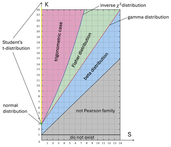
Figure 1. Some distributions from the Pearson family in the $S-K$ plot. Figure created by A. Logachov and A. Yambartsev.

This article emerged as a result of addressing the following question: How does the $JB$ statistic change when the researcher knows the following?

• The mean of the population distribution (the variance is unknown);
• The variance of the population distribution (the mean is unknown);
• The mean and variance of the population distribution.

In the last case, the known mean and variance lead us to the known coefficient of variation. For a discussion on inference when the coefficient of variation is known, we refer the reader to [5,6], and the references therein.

In this paper, we adapt the $JB$ statistic for cases where one or both normal distribution parameters are known. As simulations show, the proposed tests also demonstrate good power for many samples not belonging to the Pearson family of distributions.

To conclude this section, we note the following: In practical research, knowing the parameters of the normal distribution is crucial, as it allows us to estimate the probabilities of desired events. Testing the hypothesis of normality with specific parameters is significant because any deviation—whether in the form of outliers (deviations from normality) or change points in stochastic processes (a sudden change in the parameter)—can indicate the presence of unusual or catastrophic events. For example, small but significant parameter changes can signal a disturbance in the production process. Strong and rare deviations are of particular interest when studying stochastic processes with catastrophes. We believe a deeper connection exists between these seemingly distinct fields, which still awaits thorough investigation.

The rest of this paper is organized as follows. The following section, Section 2, presents the main results (the limit theorem and criteria for testing the corresponding statistical hypotheses). In Section 3, we present a Monte Carlo simulation to compare the suggested tests with some existing procedures. We prove Theorem 1 in Section 4. Finally, the last section contains tables of test power resulting from the Monte Carlo numerical simulations.

2. Definitions and Results

Let $X_1,X_2,\dots ,X_n,n\in \mathbb{N}$ be i.i.d. random variables on the same probability space $(\Omega ,\mathfrak{F},\mathbf{P})$. We use $\mathbf{E}$ and $\mathbf{D}$ to denote expectation and variance with respect to the probability measure $\mathbf{P}$. The convergence in distribution we denote as $\stackrel{d}{\underset{n\to \infty }{⟶}}$.

Recall the definition of empirical skewness, S, and kurtosis, K:

$$S={\displaystyle \frac{\frac{1}{n}{\displaystyle \sum _{i=1}^n}{(X_i-\overline{X})}^3}{{\widehat{\sigma }}^3}},K={\displaystyle \frac{\frac{1}{n}{\displaystyle \sum _{i=1}^n}{(X_i-\overline{X})}^4}{{\widehat{\sigma }}^4}},$$

where, as usual, we have the following:

$$\widehat{\sigma }={\left({\displaystyle \frac{1}{n}}{\displaystyle \sum _{i=1}^n}{(X_i-\overline{X})}^2\right)}^{{\displaystyle \frac{1}{2}}},\overline{X}={\displaystyle \frac{1}{n}}{\displaystyle \sum _{i=1}^n}{X}_i.$$

The main result is as follows:

Theorem 1.

Let $X,X_1,\cdots ,X_n$, $n\in \mathbb{N}$ be i.i.d. random variables. Then, we have the following:

(1) If X has a non-degenerate normal distribution and $\mathbf{E}X=a$, then

$$J{B}_a=n\left({\displaystyle \frac{S_a^2}{15}}+{\displaystyle \frac{{(K_a-3)}^2}{24}}\right)\stackrel{d}{\underset{n\to \infty }{⟶}}Y\sim {\chi }^2\left(2\right),$$

where

$$S_a={\displaystyle \frac{\frac{1}{n}{\displaystyle \sum _{i=1}^n}{(X_i-a)}^3}{{\widehat{\sigma }}_a^3}},K_a={\displaystyle \frac{\frac{1}{n}{\displaystyle \sum _{i=1}^n}{(X_i-a)}^4}{{\widehat{\sigma }}_a^4}},{\widehat{\sigma }}_a={\left({\displaystyle \frac{1}{n}}{\displaystyle \sum _{i=1}^n}{(X_i-a)}^2\right)}^{{\displaystyle \frac{1}{2}}};$$

(2) If X has a normal distribution and $\mathbf{D}X={\sigma }^2>0$, then

$$J{B}_{{\sigma }^2}=n\left({\displaystyle \frac{S_{{\sigma }^2}^2}{6}}+{\displaystyle \frac{{(K_{{\sigma }^2}-3)}^2}{96}}\right)\stackrel{d}{\underset{n\to \infty }{⟶}}Y\sim {\chi }^2\left(2\right),$$

where

$$S_{{\sigma }^2}={\displaystyle \frac{\frac{1}{n}{\displaystyle \sum _{i=1}^n}{(X_i-\overline{X})}^3}{{\sigma }^3}},K_{{\sigma }^2}={\displaystyle \frac{\frac{1}{n}{\displaystyle \sum _{i=1}^n}{(X_i-\overline{X})}^4}{{\sigma }^4}};$$

(3) If X has a normal distribution with $\mathbf{E}X=a$ and $\mathbf{D}X={\sigma }^2>0$, then

$$J{B}_{a,{\sigma }^2}=n\left({\displaystyle \frac{S_{a,{\sigma }^2}^2}{15}}+{\displaystyle \frac{{(K_{a,{\sigma }^2}-3)}^2}{96}}\right)\stackrel{d}{\underset{n\to \infty }{⟶}}Y\sim {\chi }^2\left(2\right),$$

where

$$S_{a,{\sigma }^2}={\displaystyle \frac{\frac{1}{n}{\displaystyle \sum _{i=1}^n}{(X_i-a)}^3}{{\sigma }^3}},K_{a,{\sigma }^2}={\displaystyle \frac{\frac{1}{n}{\displaystyle \sum _{i=1}^n}{(X_i-a)}^4}{{\sigma }^4}}.$$

Theorem 1 yields the following asymptotic tests. Let $\alpha$ be the significance level. Recall that ${\chi }_{1-\alpha }^2\left(2\right)$ denotes the $1-\alpha$ quantile of the ${\chi }^2\left(2\right)$ distribution.

• If we test the null hypothesis $H_0:X_i\sim N(a,{\sigma }^2),1\le i\le n,$ (where a is known and ${\sigma }^2$ is unknown) against the alternative hypothesis $H_1:X_i$ follows a distribution from the Pearson family that is not normal but has a mean equal to a. Then, from statement (1) of Theorem 1, for a sufficiently large sample size, the following rule can be used: if $J{B}_a<{\chi }_{1-\alpha }^2\left(2\right)$, then the null hypothesis $H_0$ is accepted; otherwise, it is rejected.
• When we test the null hypothesis $H_0:X_i\sim N(a,{\sigma }^2),1\le i\le n,$ (where a is unknown and ${\sigma }^2$ is known) against the alternative $H_1:X_i$ follows a distribution from the Pearson family that is not normal with variance equal to ${\sigma }^2$. Then, from statement (2) of Theorem 1, for a sufficiently large sample size, the following rule can be used: if $J{B}_{{\sigma }^2}<{\chi }_{1-\alpha }^2\left(2\right)$, then the null hypothesis $H_0$ is accepted; otherwise, it is rejected.
• When the null hypothesis $H_0:X_i\sim N(a,{\sigma }^2),1\le i\le n,$ (a and ${\sigma }^2$ are known) is tested against the alternative $H_1:X_i$ follows a distribution from the Pearson family that is not $N(a,{\sigma }^2)$. Then, from statement (3) of Theorem 1, for a sufficiently large sample size, the following testing rule can be applied: if $J{B}_{a,{\sigma }^2}<{\chi }_{1-\alpha }^2\left(2\right)$, then the null hypothesis $H_0$ is accepted; otherwise, it is rejected.

It should also be noted that the above tests are goodness-of-fit tests, i.e., if the alternative hypothesis $H_1$ holds for the sample elements, then the values of the corresponding statistics $J{B}_a$, $J{B}_{{\sigma }^2}$, and $J{B}_{a,{\sigma }^2}$ converge in probability to ∞ as $n\to \infty$.

3. Simulation Study

In this section, we compare the power of various tests for normality using Monte Carlo simulations of alternative hypotheses. The simulations were performed in R software, version 4.2.3. We used the following sample sizes (small, moderate, and large): $n=25,50,75,100,150,200,250,500$, and 1000. The null hypothesis is $N(0,1)$ in almost all cases; we specify separately where this is not the case. As alternative hypotheses, we considered normal, log-normal, mixed normal, Student, gamma, and uniform distributions. Note that the log-normal and mixed normal distributions do not belong to the Pearson family of distributions and uniform distribution is the limit of the Pearson type I distribution. All codes are written in R and available at https://github.com/KhrushchevSergey/Modified-Jarque-Bera-test, accessed on 1 June 2024.

Here, we consider the following tests for normality:

• Kolmogorov–Smirnov (KS) test. The test statistic measures the maximum deviation between the theoretical cumulative distribution function and the empirical cumulative distribution function. When the parameters of the normal distribution are unknown, they are estimated from the sample and used in the test.
• Anderson–Darling (AD) test. The Anderson–Darling test assesses whether a sample comes from a specific distribution, often the normal distribution. It gives more weight to the tails of the distribution compared to other tests, making it sensitive to deviations from normality in those areas.
• Cramér–von Mises (CVM) test. The Cramér–von Mises test, like the KS test, is based on the distance between the empirical and specified theoretical distributions. It measures the cumulative squared differences between the empirical and theoretical cumulative distribution functions, providing a robust assessment of overall fit.
• Lilliefors (LF) Kolmogorov–Smirnov test. The Lilliefors test is based on the Kolmogorov–Smirnov test. It tests the null hypothesis that data come from a normally distributed population without specifying the parameters.
• Shapiro–Wilk (SW) test. The Shapiro–Wilk test is one of the most popular tests with good power. It is based on a correlation between given observations and associated normal scores.

We estimate the power in the following way. For the given n, we generate 1000 samples with the sample size n according to the alternative hypothesis. The empirical power is the ratio of the number of rejections of the null hypothesis to 1000. We categorize our findings based on the following cases of the alternative hypothesis distribution.

3.1. Normal versus Normal

• Different variances and the same means. We start by comparing the test powers when the alternative distribution is the normal distribution with a zero mean and a variance different from one, specifically, $N(0,2)$. See Table A1. Since we considered two normal distributions with different variances but the same mean, we added the column with the power of the Fisher test. The Fisher test checks the hypothesis if the variance is equal to one. We expect that, in this situation, the modified Jarque–Bera statistic would exhibit the highest power. The KS and CVM statistics have demonstrated similarly lower power, while the power of the AD statistic falls between that of the KS, CVM, and modified Jarque–Bera statistics.
• Different means and the same variances. Here, we compare the test powers when the alternative distribution is a normal distribution with a mean of one and a variance of one, $N(1,1)$. See Table A2. Since two normal distributions with different means but the same variance are considered, we added two additional columns with the test powers of the Student and Welch tests, respectively. All statistics perform similarly well, except for the modified Jarque–Bera with a known mean for the small sample sizes.

3.2. Normal versus Student’s t with Degrees of Freedom 1 (Cauchy), 5, and 9

• Cauchy. Here, consider the case where the alternative distribution is the Cauchy distribution. See Table A3. Since the alternative distribution is not normal, we did not conduct additional tests such as the Student or Fisher tests. In this case, the $J_{a,{\sigma }^2}$ test provided the best power, but all tests performed similarly well, except for the Kolmogorov–Smirnov and the Cramér–von Mises tests. Since the normal distribution differs significantly from the Cauchy distribution, almost all tests provided good power.
• Student’s t-distribution with 5 and 9 degrees of freedom. Here, we consider the comparison between the test powers when the alternative distribution is the $t_{\nu }$ distribution with $\nu =5$. In contrast to the Cauchy distribution, the Student’s t distribution is more similar to the normal distribution, so the expected values of the powers are smaller than in the Cauchy case. Moreover, the $J_{a,{\sigma }^2}$ statistic provided significantly better power. See Table A4. Since the Student’s t distribution with $\nu =9$ is even more similar to the standard normal distribution, the power will be smaller with similar relationships between different tests. Therefore, we omitted the entire table of powers. To give an idea about the magnitude of the changes in power, for the $J_{a,{\sigma }^2}$ statistic with $n=25$ and $\alpha =0.05$, the power changed from $0.56$ to $0.34$. Note that the KS test exhibited the worst power. Additionally, observe that the performance of $J_a$ is worse than those of $J_{a,{\sigma }^2}$ and $J_{{\sigma }^2}$. This, of course, is expected because the null and alternative distributions have the same zero mean. Note that the $A{D}_c$, $CV{M}_c$, and $SW$ statistics exhibited power lower than but comparable to those of all the Jarque–Bera statistics. For this case, for Student’s t with 5 degrees of freedom, we plotted the test power for both $\alpha$ values to provide a more detailed breakdown of these power comparisons. See Figure A1 and Figure A2 in Appendix A.

3.3. Normal versus Non-Symmetric and Non-Pearson Type Distributions

• For non-symmetric alternative distributions, (i) the gamma (2,1), $\gamma (2,1)$, (ii) log-normal (0,1), and $LN(0,1)$ were considered; for non-Pearson type alternative distributions, we considered (iii) the uniform on interval $[-3,3]$, $U[-3,3]$, and (iv) the mixture of standard normal $N(0,1)$ and normal $N(0,9)$ distributions with the same mixture weights, denoted by $Mix$. Since all alternative distributions are “significantly different” from the standard normal distribution, all tables “are similar” to that of the Cauchy distribution. See Table A5, Table A6, Table A7 and Table A8. It is expected that the $J{B}_a$ statistic will lose power under symmetric alternative distributions. Moreover, the $AD$ statistic is likely to perform comparably well to the Jarque–Bera statistics $J{B}_{a,{\sigma }^2}$ and $J{B}_{{\sigma }^2}$. See Table A5 and Table A8. In the non-symmetric case (Table A6 and Table A7), the $KS$, $AD$, $CVM$, and $SW$ statistics exhibit similar high power to the modified Jarque–Bera statistic, $J{B}_{a,{\sigma }^2}$.

3.4. Normal versus Gamma Distribution with the Same Mean Value

• Finally, we decided to perform the comparison between test powers when the null hypothesis was not a standard normal distribution. Here, we test the normal distribution $N(2,2)$ versus gamma distribution $\gamma (2,1)$, which has a mean value of 2. The results are presented in Table A9. In this case, as before, the modified $J{B}_{a,{\sigma }^2}$, $J{B}_{{\sigma }^2}$, and $AD$ statistics exhibit the highest power, while the $KS$, $CVM$, and $SW$ statistics show a loss in power.

3.5. Robustness in the Presence of Outliers

• To evaluate the performance of the modified Jarque–Bera tests in the presence of outliers, we generated data from a mixture of a standard normal distribution (weight 0.9) and a sum of independent random variables—one with a standard normal distribution and the other with a Poisson distribution with a mean of 5 (weight 0.1). This type of mixture is rarely used in simulation studies, but such discrete-value outliers can occur due to failures in production machines, for example; see Table A10. In this case, the KS and CVM tests showed the lowest power performance. The modified Jarque–Bera tests showed the best power, while the other tests ($JB$, $LF$, $AD$, $A{D}_c$, $CV{M}_c$, and $SW$) had lower but similar power. We also refer the readers to [7] for robust modifications to the Jarque–Bera statistic.

3.6. Application to Real Data

We tested the hypothesis that the mass of penguins, based on their species and gender, follows a normal distribution. We applied a modified Jarque–Bera test, using the sample mean and variance as known values. The observations were taken from a popular dataset featuring penguin characteristics from the study [8], where sexual size dimorphism (SSD), i.e., ecological sexual dimorphism, was studied in penguin populations. The normal variability of penguin mass is well-accepted, thus, accepting the null hypothesis is anticipated for this dataset. The corresponding p-values are provided in the table below.

Species	Male	Female
Adelie	0.7787	0.7361
Chinstrap	0.9194	0.5876
Gentoo	0.9598	0.7687

In the next section, we provide the detailed proof of our main results.

4. Proof of Theorem 1

Let us prove proposition (1) of the theorem. Consider the sequence of random variables, as follows:

$${\overrightarrow{Z}}_n:=(Z_{1,n},Z_{2,n}):=({\displaystyle \frac{\frac{1}{\sqrt{n}}{\displaystyle \sum _{i=1}^n}{(X_i-a)}^3}{{\widehat{\sigma }}_a^3}},{\displaystyle \frac{\frac{1}{\sqrt{n}}{\displaystyle \sum _{i=1}^n}({(X_i-a)}^4-3{\widehat{\sigma }}_a^4)}{{\widehat{\sigma }}_a^4}}).$$

From the convergence, i.e.,

$$\underset{n\to \infty }{lim}{\widehat{\sigma }}_a=\sigma >0\mathrm{a}.\mathrm{s}.$$

and Slutsky’s theorem [9], it follows that the limiting distribution of the sequence ${\overrightarrow{Z}}_n$ coincides with the limiting distribution of the sequence

$${\overrightarrow{Z^{\prime }}}_n:=(Z_{1,n}^{\prime },Z_{2,n}^{\prime }):=({\displaystyle \frac{\frac{1}{\sqrt{n}}{\displaystyle \sum _{i=1}^n}{(X_i-a)}^3}{{\sigma }^3}},{\displaystyle \frac{\frac{1}{\sqrt{n}}{\displaystyle \sum _{i=1}^n}({(X_i-a)}^4-3{\widehat{\sigma }}_a^4)}{{\sigma }^4}}).$$

It is easy to see the following:

$$\begin{array}{cc}\hfill {\displaystyle \frac{1}{\sqrt{n}}}& {\displaystyle \sum _{i=1}^n}({(X_i-a)}^4-3{\widehat{\sigma }}_a^4)={\displaystyle \frac{1}{\sqrt{n}}}{\displaystyle \sum _{i=1}^n}\left({(X_i-a)}^4-3{\left({\displaystyle \frac{1}{n}}{\displaystyle \sum _{j=1}^n}{(X_j-a)}^2\right)}^2\pm 3{\sigma }^4\right)\hfill \\ & ={\displaystyle \frac{1}{\sqrt{n}}}{\displaystyle \sum _{i=1}^n}\left({(X_i-a)}^4-3{\sigma }^4+3\left({\sigma }^2-{\displaystyle \frac{1}{n}}{\displaystyle \sum _{j=1}^n}{(X_j-a)}^2\right)\left({\sigma }^2+{\displaystyle \frac{1}{n}}{\displaystyle \sum _{j=1}^n}{(X_j-a)}^2\right)\right)\hfill \\ & ={\displaystyle \frac{1}{\sqrt{n}}}{\displaystyle \sum _{i=1}^n}\left({(X_i-a)}^4-3{\sigma }^4+3\left({\sigma }^2-{\displaystyle \frac{1}{n}}{\displaystyle \sum _{j=1}^n}{(X_j-a)}^2\right)\left(2{\sigma }^2+\left({\displaystyle \frac{1}{n}}{\displaystyle \sum _{j=1}^n}{(X_j-a)}^2-{\sigma }^2\right)\right)\right)\hfill \\ & ={\displaystyle \frac{1}{\sqrt{n}}}{\displaystyle \sum _{i=1}^n}\left({(X_i-a)}^4-3{\sigma }^4+6{\sigma }^2\left({\sigma }^2-{\displaystyle \frac{1}{n}}{\displaystyle \sum _{j=1}^n}{(X_j-a)}^2\right)\right)-{\displaystyle \frac{3}{\sqrt{n}}}{\displaystyle \sum _{i=1}^n}{\left({\sigma }^2-{\displaystyle \frac{1}{n}}{\displaystyle \sum _{j=1}^n}{(X_j-a)}^2\right)}^2\hfill \\ & ={\displaystyle \frac{1}{\sqrt{n}}}{\displaystyle \sum _{i=1}^n}\left({(X_i-a)}^4+3{\sigma }^4-6{\sigma }^2{(X_i-a)}^2\right)-3\sqrt{n}{\left({\displaystyle \frac{1}{n}}{\displaystyle \sum _{j=1}^n}({\sigma }^2-{(X_j-a)}^2)\right)}^2\hfill \\ & ={\displaystyle \frac{1}{\sqrt{n}}}{\displaystyle \sum _{i=1}^n}\left({(X_i-a)}^4+3{\sigma }^4-6{\sigma }^2{(X_i-a)}^2\right)-3{\left({\displaystyle \frac{1}{n^{\frac{3}{4}}}}{\displaystyle \sum _{j=1}^n}({\sigma }^2-{(X_j-a)}^2)\right)}^2.\hfill \end{array}$$

The law of the iterative logarithm yields the following:

$$\underset{n\to \infty }{lim}{\displaystyle \frac{1}{n^{\frac{3}{4}}}}{\displaystyle \sum _{j=1}^n}({\sigma }^2-{(X_j-a)}^2)=0\mathrm{a}.\mathrm{s}.$$

Therefore, applying Slutsky’s theorem, we can conclude that the limiting distribution of the sequence ${\overrightarrow{Z^{\prime }}}_n$ coincides with the limiting distribution of the sequence, as follows:

$$\begin{array}{cc}\hfill {\overrightarrow{Z^{\prime \prime }}}_n:=(Z_{1,n}^{\prime },Z_{2,n}^{\prime \prime }):=& ({\displaystyle \frac{\frac{1}{\sqrt{n}}{\displaystyle \sum _{i=1}^n}{(X_i-a)}^3}{{\sigma }^3}},{\displaystyle \frac{\frac{1}{\sqrt{n}}{\displaystyle \sum _{i=1}^n}({(X_i-a)}^4-6{\sigma }^2{(X_i-a)}^2+3{\sigma }^4)}{{\sigma }^4}})\hfill \\ \hfill =& {\displaystyle \frac{1}{\sqrt{n}}}{\displaystyle \sum _{i=1}^n}({\displaystyle \frac{{(X_i-a)}^3}{{\sigma }^3}},{\displaystyle \frac{{(X_i-a)}^4-6{\sigma }^2{(X_i-a)}^2+3{\sigma }^4}{{\sigma }^4}}).\hfill \end{array}$$

By the central limit theorem, the sequence ${\overrightarrow{Z^{\prime \prime }}}_n$ converges to the random vector $(W_1,W_2)$, whose coordinates have a joint normal distribution. Therefore, it suffices to show that these coordinates are uncorrelated and have the required variances.

It is easy to see that $\mathbf{D}{(X_i-a)}^3=15{\sigma }^6$ (thus, $\mathbf{D}{W}_1=15$); $\mathbf{D}({(X_i-a)}^4-6{\sigma }^2{(X_i-a)}^2+3{\sigma }^4)=24{\sigma }^8$ (thus $\mathbf{D}{W}_2=24$). From the fact that the odd moments of a centered normally distributed random variable are equal to zero, it follows that

$$\mathbf{E}\left({\displaystyle \frac{{(X_i-a)}^3}{{\sigma }^3}}·{\displaystyle \frac{{(X_i-a)}^4-6{\sigma }^2{(X_i-a)}^2+3{\sigma }^4}{{\sigma }^4}}\right)=0$$

(therefore, $\mathbf{E}{W}_1{W}_2=0$).

Therefore, we have shown that $(W_1,W_2)$ has a joint normal distribution with a covariance matrix, as follows:

$$\Sigma =\left(\begin{array}{cc}15& 0\\ 0& 24\end{array}\right).$$

Thus,

$${\displaystyle \frac{W_1^2}{15}}+{\displaystyle \frac{W_2^2}{24}}\sim {\chi }^2\left(2\right).$$

Let us prove statement (2). Consider the following sequence of random vectors:

$${\overrightarrow{Z}}_n:=(Z_{1,n},Z_{2,n}):=({\displaystyle \frac{\frac{1}{\sqrt{n}}{\displaystyle \sum _{i=1}^n}{(X_i-\overline{X})}^3}{{\sigma }^3}},{\displaystyle \frac{\frac{1}{\sqrt{n}}{\displaystyle \sum _{i=1}^n}({(X_i-\overline{X})}^4-3{\sigma }^4)}{{\sigma }^4}}).$$

It is easy to see the following:

$$\begin{array}{cc}\hfill {\displaystyle \frac{1}{\sqrt{n}}}& {\displaystyle \sum _{i=1}^n}{(X_i-\overline{X})}^3={\displaystyle \frac{1}{\sqrt{n}}}{\displaystyle \sum _{i=1}^n}{((X_i-a)-(\overline{X}-a))}^3={\displaystyle \frac{1}{\sqrt{n}}}{\displaystyle \sum _{i=1}^n}{\left((X_i-a)-{\displaystyle \frac{1}{n}}{\displaystyle \sum _{j=1}^n}(X_j-a)\right)}^3\hfill \\ \hfill =& {\displaystyle \frac{1}{\sqrt{n}}}{\displaystyle \sum _{i=1}^n}{(X_i-a)}^3-{\displaystyle \frac{3}{\sqrt{n}}}{\displaystyle \sum _{i=1}^n}{(X_i-a)}^2·{\displaystyle \frac{1}{n}}{\displaystyle \sum _{j=1}^n}(X_j-a)\hfill \\ & +{\displaystyle \frac{3}{\sqrt{n}}}{\displaystyle \sum _{i=1}^n}(X_i-a)·{\left({\displaystyle \frac{1}{n}}{\displaystyle \sum _{j=1}^n}(X_j-a)\right)}^2-\sqrt{n}{\left({\displaystyle \frac{1}{n}}{\displaystyle \sum _{j=1}^n}(X_j-a)\right)}^3\hfill \\ \hfill =& {\displaystyle \frac{1}{\sqrt{n}}}{\displaystyle \sum _{i=1}^n}{(X_i-a)}^3-\left({\displaystyle \frac{1}{n}}{\displaystyle \sum _{i=1}^n}{(X_i-a)}^2\right)·{\displaystyle \frac{3}{\sqrt{n}}}{\displaystyle \sum _{j=1}^n}(X_j-a)\hfill \\ & +{\displaystyle \frac{3}{n}}{\displaystyle \sum _{i=1}^n}(X_i-a)·{\left({\displaystyle \frac{1}{n^{\frac{3}{4}}}}{\displaystyle \sum _{j=1}^n}(X_j-a)\right)}^2-{\left({\displaystyle \frac{1}{n^{\frac{5}{6}}}}{\displaystyle \sum _{j=1}^n}(X_j-a)\right)}^3\hfill \end{array}$$

Finally, introducing $g_{1,n},g_{1,n}$ and $g_{3,n}$ we have the following:

$${\displaystyle \frac{1}{\sqrt{n}}}{\displaystyle \sum _{i=1}^n}{(X_i-\overline{X})}^3=:{\displaystyle \frac{1}{\sqrt{n}}}{\displaystyle \sum _{i=1}^n}{(X_i-a)}^3-g_{1,n}·{\displaystyle \frac{3}{\sqrt{n}}}{\displaystyle \sum _{j=1}^n}(X_j-a)+g_{2,n}-g_{3,n}.$$

(1)

The law of large numbers and the law of the iterated logarithm yield the following:

$$\underset{n\to \infty }{lim}{g}_{1,n}={\sigma }^2\mathrm{a}.\mathrm{s}.and\underset{n\to \infty }{lim}{g}_{3,n}=0\mathrm{a}.\mathrm{s}.$$

(2)

The sequences ${\displaystyle \frac{3}{n}}{\displaystyle \sum _{i=1}^n}(X_i-a)$ and ${\displaystyle \frac{1}{n^{\frac{3}{4}}}}{\displaystyle \sum _{j=1}^n}(X_j-a)$ converge almost surely to zero as $n\to \infty$, due to the law of large numbers and the law of the iterated logarithm, respectively; therefore, we have the following:

$$\underset{n\to \infty }{lim}{g}_{2,n}=0\mathrm{a}.\mathrm{s}.$$

(3)

Let us consider the numerator of the second coordinate of the random vector as follows:

$$\begin{array}{cc}\hfill {\displaystyle \frac{1}{\sqrt{n}}}& {\displaystyle \sum _{i=1}^n}{(X_i-\overline{X})}^4={\displaystyle \frac{1}{\sqrt{n}}}{\displaystyle \sum _{i=1}^n}{((X_i-a)-(\overline{X}-a))}^4={\displaystyle \frac{1}{\sqrt{n}}}{\displaystyle \sum _{i=1}^n}{\left((X_i-a)-{\displaystyle \frac{1}{n}}{\displaystyle \sum _{j=1}^n}(X_j-a)\right)}^4\hfill \\ \hfill =& {\displaystyle \frac{1}{\sqrt{n}}}{\displaystyle \sum _{i=1}^n}{(X_i-a)}^4-{\displaystyle \frac{4}{\sqrt{n}}}{\displaystyle \sum _{i=1}^n}{(X_i-a)}^3·{\displaystyle \frac{1}{n}}{\displaystyle \sum _{j=1}^n}(X_j-a)+{\displaystyle \frac{6}{\sqrt{n}}}{\displaystyle \sum _{i=1}^n}{(X_i-a)}^2·{\left({\displaystyle \frac{1}{n}}{\displaystyle \sum _{j=1}^n}(X_j-a)\right)}^2\hfill \\ & -{\displaystyle \frac{4}{\sqrt{n}}}{\displaystyle \sum _{i=1}^n}(X_i-a)·{\left({\displaystyle \frac{1}{n}}{\displaystyle \sum _{j=1}^n}(X_j-a)\right)}^3+\sqrt{n}{\left({\displaystyle \frac{1}{n}}{\displaystyle \sum _{j=1}^n}(X_j-a)\right)}^4\hfill \\ \hfill =& {\displaystyle \frac{1}{\sqrt{n}}}{\displaystyle \sum _{i=1}^n}{(X_i-a)}^4-{\displaystyle \frac{4}{n^{\frac{3}{4}}}}{\displaystyle \sum _{i=1}^n}{(X_i-a)}^3·{\displaystyle \frac{1}{n^{\frac{3}{4}}}}{\displaystyle \sum _{j=1}^n}(X_j-a)+{\displaystyle \frac{6}{n}}{\displaystyle \sum _{i=1}^n}{(X_i-a)}^2·{\left({\displaystyle \frac{1}{n^{\frac{3}{4}}}}{\displaystyle \sum _{j=1}^n}(X_j-a)\right)}^2\hfill \\ & -{\displaystyle \frac{4}{n}}{\displaystyle \sum _{i=1}^n}(X_i-a)·{\left({\displaystyle \frac{1}{n^{\frac{5}{6}}}}{\displaystyle \sum _{j=1}^n}(X_j-a)\right)}^3+{\left({\displaystyle \frac{1}{n^{\frac{7}{8}}}}{\displaystyle \sum _{j=1}^n}(X_j-a)\right)}^4.\hfill \end{array}$$

Denoting $g_{4,n}$, the four last terms, we have the following:

$${\displaystyle \frac{1}{\sqrt{n}}}{\displaystyle \sum _{i=1}^n}{(X_i-\overline{X})}^4=:{\displaystyle \frac{1}{\sqrt{n}}}{\displaystyle \sum _{i=1}^n}{(X_i-a)}^4+g_{4,n}.$$

(4)

From the law of large numbers and the law of the iterated logarithm, we have the following:

$$\underset{n\to \infty }{lim}{g}_{4,n}=0\mathrm{a}.\mathrm{s}.$$

(5)

From (1)–(5) and Slutsky’s theorem, it follows that the limiting distribution of the sequence ${\overrightarrow{Z}}_n$ coincides with the limiting distribution of the sequence, as follows:

$${\overrightarrow{Z^{\prime }}}_n:=(Z_{1,n}^{\prime },Z_{2,n}^{\prime }):=({\displaystyle \frac{\frac{1}{\sqrt{n}}{\displaystyle \sum _{i=1}^n}({(X_i-a)}^3-3{\sigma }^2(X_i-a))}{{\sigma }^3}},{\displaystyle \frac{\frac{1}{\sqrt{n}}{\displaystyle \sum _{i=1}^n}({(X_i-a)}^4-3{\sigma }^4)}{{\sigma }^4}})$$

$$={\displaystyle \frac{1}{\sqrt{n}}}{\displaystyle \sum _{i=1}^n}({\displaystyle \frac{{(X_i-a)}^3-3{\sigma }^2(X_i-a)}{{\sigma }^3}},{\displaystyle \frac{{(X_i-a)}^4-3{\sigma }^4}{{\sigma }^4}}).$$

By the central limit theorem, the sequence ${\overrightarrow{Z^{\prime }}}_n$ converges to the random vector $(W_1,W_2)$, whose coordinates have a joint normal distribution with a covariance matrix, as follows:

$$\Sigma =\left(\begin{array}{cc}\mathbf{D}{W}_1& \mathbf{E}{W}_1{W}_2\\ \mathbf{E}{W}_1{W}_2& \mathbf{D}{W}_2\end{array}\right).$$

It is easy to see that $\mathbf{D}({(X_i-a)}^3-3{\sigma }^2(X_i-a))=6{\sigma }^6$ (thus, $\mathbf{D}{W}_1=6$); $\mathbf{D}({(X_i-a)}^4-3{\sigma }^4)=96{\sigma }^8$ (thus, $\mathbf{D}{W}_2=96$). From the fact that the odd moments of a centered normally distributed random variable are equal to zero, we derive the following:

$$\mathbf{E}\left({\displaystyle \frac{{(X_i-a)}^3-3{\sigma }^2(X_i-a)}{{\sigma }^3}}·{\displaystyle \frac{{(X_i-a)}^4-3{\sigma }^4}{{\sigma }^4}}\right)=0$$

(and, thus, $\mathbf{E}{W}_1{W}_2=0$). Therefore,

$${\displaystyle \frac{W_1^2}{6}}+{\displaystyle \frac{W_2^2}{96}}\sim {\chi }^2\left(2\right).$$

Proof. 

The proof of statement (3) is similar (just simpler since a and ${\sigma }^2$ are known), so we omit it. □

5. Conclusions

In this paper, new modifications to the Jarque–Bera statistics are proposed. Detailed proofs are provided, which are simple and accessible even to undergraduate students in probability and statistics.

A Monte Carlo study showed that the Jarque–Bera statistic and its new modifications perform well on the class of Pearson distributions. When the alternative distribution does not belong to the Pearson family, Jarque–Bera and its modifications perform well alongside other statistics such as Anderson–Darling, Cramér–von Mises, and Shapiro–Wilk. Like any specific test, the Jarque–Bera test and its modifications have natural limitations in their application. Despite the test performing well on classical distributions, a significant drawback is that it cannot distinguish between symmetric distributions with a kurtosis of 3.

Our goal was not to explore and compare all existing tests; therefore, we limited our comparison to the most widely used tests for normality. Comparative studies on a broader class of normality tests can be found in [10,11]. Note that the findings of [10,11] are aligned with our simulation results. For more comparative studies, we also refer to [12].

In this paper, we are limited to the univariate case. Multivariate normality tests represent a curious and interesting area of research. For discussions on existing tests and the possibility of multivariate extensions of some known statistics, including Jarque–Bera we refer the readers to [12,13], and the references therein.

References

- Jarque, C.M.; Bera, A.K. Efficient tests for normality, homoscedasticity and serial independence of regression residuals. Econ. Lett. 1980, 6, 255–259. [Google Scholar] [CrossRef]
- Jarque, C.M.; Bera, A.K. Efficient tests for normality, homoscedasticity and serial independence of regression residuals: Monte Carlo evidence. Econ. Lett. 1981, 7, 313–318. [Google Scholar] [CrossRef]
- Jarque, C.M.; Bera, A.K. A test for normality of observations and regression residuals. Int. Stat. Rev. 1987, 55, 163–172. [Google Scholar] [CrossRef]
- Pearson, K. Mathematical contributions to the theory of evolution, XIX: Second supplement to a memoir on skew variation. Philos. Trans. R. Soc. A 1916, 216, 429–457. [Google Scholar]
- Searls, D.T. The utilization of a known coefficient of variation in the estimation procedure. J. Am. Stat. Assoc. 1964, 59, 1225–1226. [Google Scholar] [CrossRef]
- Fu, Y.; Wang, H.; Wong, A. Inference for the normal mean with known coefficient of variation. Open J. Stat. 2013, 3, 41368. [Google Scholar] [CrossRef]
- Rana, S.; Eshita, N.N.; Al Mamun, A.S.M. Robust normality test in the presence of outliers. J. Phys. Conf. Ser. 2021, 1863, 012009. [Google Scholar] [CrossRef]
- Gorman, K.B.; Williams, T.D.; Fraser, W.R. Ecological Sexual Dimorphism and Environmental Variability within a Community of Antarctic Penguins (Genus Pygoscelis). PLoS ONE 2014, 9, e90081. [Google Scholar] [CrossRef] [PubMed]
- Slutsky, E. Über stochastische Asymptoten und Grenzwerte. Metron 1925, 5, 3–89. [Google Scholar]
- Yap, B.W.; Sim, C.H. Comparisons of various types of normality tests. J. Stat. Comput. Simul. 2011, 81, 2141–2155. [Google Scholar] [CrossRef]
- Razali, N.M.; Wah, Y.B. Power comparisons of shapiro-wilk, kolmogorov-smirnov, lilliefors and anderson-darling tests. J. Stat. Model. Anal. 2011, 2, 21–33. [Google Scholar]
- Khatun, N. Applications of normality test in statistical analysis. Open J. Stat. 2021, 11, 113. [Google Scholar] [CrossRef]
- Chen, W.; Genton, M.G. Are you all normal? It depends! Int. Stat. Rev. 2023, 91, 114–139. [Google Scholar] [CrossRef]
Disclaimer/Publisher’s Note: The statements, opinions and data contained in all publications are solely those of the individual author(s) and contributor(s) and not of MDPI and/or the editor(s). MDPI and/or the editor(s) disclaim responsibility for any injury to people or property resulting from any ideas, methods, instructions or products referred to in the content. |
© 2024 by the authors. Licensee MDPI, Basel, Switzerland. This article is an open access article distributed under the terms and conditions of the Creative Commons Attribution (CC BY) license (https://creativecommons.org/licenses/by/4.0/).