Dupin Cyclides as a Subspace of Darboux Cyclides

Abstract

Dupin cyclides are interesting algebraic surfaces used in geometric design and architecture to join canal surfaces smoothly and to construct model surfaces. Dupin cyclides are special cases of Darboux cyclides, which in turn are rather general surfaces in ${\mathbb{R}}^3$ of degree 3 or 4. This article derives the algebraic conditions for the recognition of Dupin cyclides among the general implicit form of Darboux cyclides. We aim at practicable sets of algebraic equations on the coefficients of the implicit equation, each such set defining a complete intersection (of codimension 4) locally. Additionally, the article classifies all real surfaces and lower-dimensional degenerations defined by the implicit equation for Dupin cyclides.

1. Introduction

Darboux cyclides are classical algebraic surfaces in ${\mathbb{R}}^3$ that have promising applications in geometric design and architecture. Their implicit equation has the form

$$\begin{array}{cc}\hfill a_0{\left(x^2+y^2+z^2\right)}^2& +2(b_{1}x+b_{2}y+b_{3}z)\left(x^2+y^2+z^2\right)\hfill \\ \hfill & +c_1{x}^2+c_2{y}^2+c_3{z}^2+2d_{1}yz+2d_{2}xz+2d_{3}xy\hfill \\ \hfill & +2e_{1}x+2e_{2}y+2e_{3}z+f_0=0.\hfill \end{array}$$

(1)

Here, $a_0,b_1,\dots ,f_0$ are real coefficients. Remarkably, Darboux cyclides are covered by several families of circles [1,2,3]. Hence, they are natural candidates to model a surface composed of patches blended along circles. This task is still challenging for more general Darboux cyclides [4], but the special cases of Darboux cyclides called Dupin cyclides have definite applications already [5,6,7,8,9,10,11,12]. Conveniently, Dupin cyclides are canal surfaces whose curvature lines are circles or lines. They are useful to join pipes between canal surfaces [8] and to model surfaces smoothly blended along curvature lines [9,10,11,12]. Significantly, the set of Dupin cyclides is stable under the offsetting at a fixed distance along the surface normals [6,11,13]. The offset operation arises frequently in geometric design and manufacturing [2,6]. On that account, geometric modeling with Dupin cyclides simplifies the computation of offset surfaces. The contrast between Dupin and Darboux cyclides is illustrated in Figure 1. Darboux cyclides generally have six circles through each point on the surface [14,15], while Dupin cyclides have two principal circles as lines of curvature and two so-called Villarceau circles through each point; the principal circles represent pairs of coalescing circles of the general Darboux cyclide ([2], Theorem 18(v)).

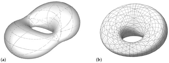
Figure 1. (a) A smooth Darboux cyclide covered by six families of circles drawn in solid, dash, dot, dashdot, spacedot, or longdash. There are two examplar points with six circles through them near the donut hole. (b) A smooth Dupin cyclide covered by four families of circles; the solid circles are principal circles and the dashed circles are Villarceau circles (see Section 6.2).

It is evidently desirable to distinguish Dupin cyclides among general Darboux cyclides. The implied standard recognition procedures involve bringing the implicit equation (1) to a known canonical form by Möbius transformations [4,16], or discerning that a geometric characterization is satisfied [12,17,18]. To establish a more convenient recognition procedure, we compute the set of algebraic equations on the coefficients $a_0,b_1,\cdots ,f_0$ characterizing Dupin cyclides among the form (1). Our starting point is the following canonical forms of Dupin cyclides under the Euclidean transformations. A quartic Dupin cyclide can be presented by the implicit equation

$${\left(x^2+y^2+z^2+{\alpha }^2-{\gamma }^2-{\delta }^2\right)}^2-4{(\alpha x-\gamma \delta )}^2-4({\alpha }^2-{\gamma }^2)y^2=0,$$

(2)

after Euclidean translations and rotations ([6], pp. 223–224), ([19], Ch. IX). We broadly assume that ${\alpha }^2$, ${\gamma }^2$, ${\delta }^2$, $\alpha \gamma \delta \in \mathbb{R}$, thereby allowing cyclides without real points along other degenerate cases. All degenerate cases are described further in Section 6.3. A cubic Dupin cyclide can be brought to the form

$$\begin{array}{c}\hfill 2x(x^2+y^2+z^2)-(p+q)x^2-p{y}^2-q{z}^2+{\displaystyle \frac{pq}{2}}x=0\end{array}$$

(3)

with $p,q\in \mathbb{R}$. This differs from the equation in ([7], p. 151) by a scaling of $p,q$ with a factor of 2. The Euclidean equivalence to these two forms replaces here the classical definition of Dupin cyclides by Möbius equivalence in ${\mathbb{R}}^3\cup \{\infty \}$ to a torus, a cylinder, or a cone [18]. We give a generic explicit Möbius isomorphism between Dupin cyclides and toruses in Section 6.1.

It is straightforward to normalize the coefficients $b_1,b_2,b_3$ to zero (if $a_0\ne 0$) by Euclidean translations, but further normalization by orthogonal or Möbius transformations is cumbersome. This article presents the computed set of necessary and (generically) sufficient algebraic conditions on $a_0,b_1,\dots ,f_0$ so that Equation (1) defines a Dupin cyclide. The problem of recognizing Dupin cyclides from an implicit equation is a complementary question to the constructive classification of Dupin and Darboux cyclides by normal forms [4] or pentaspherical projection from ${\mathbb{P}}^4$ [15]. We view the 14 coefficients in (1) as the homogeneous coordinates $(a_0:b_1:\dots :f_0)$ in the real projective space ${\mathbb{P}}^{13}$, which is identified as the space of Darboux cyclides. The Dupin cyclides are represented by the projective variety ${\mathcal{D}}_0$ in ${\mathbb{P}}^{13}$ defined by the found algebraic conditions. Some of the points on this variety represent degenerations of cyclides to reducible, non-reduced, or quadratic surfaces.

To organize the results, the cases of quartic and cubic cyclides are considered separately. The subvariety of ${\mathcal{D}}_0$ representing quartic Dupin cyclides has $a_0\ne 0$ in (1); it will be denoted by ${\mathcal{D}}_4$. The subvariety of ${\mathcal{D}}_0$ representing cubic Dupin cyclides (i.e., with $a_0=0$ and $b_1^2+b_2^2+b_3^2\ne 0$) will be denoted by ${\mathcal{D}}_3$. We are interested only in the real points on those varieties so that the coefficients in (1) are real. The next section states the main results of this article: the algebraic equations that characterize the two main subvarieties ${\mathcal{D}}_4$ and ${\mathcal{D}}_3$. The results are proven in Section 3 (for quartic cyclides) and Section 4 (for cubic cyclides).

As summarized in Section 5.2, the co-dimension of the considered spaces of Dupin cyclides inside the respective projective spaces of Darboux cyclides equals 4. In particular, the variety ${\mathcal{D}}_0$ has dimension 9. The main explicit result is presented in Theorem 1 by underscoring open subvarieties of those varieties that are complete intersections in a suitable ambient open subspace of ${\mathbb{P}}^{13}$. This way of presenting the results should be convenient for practical applications, we suggest. The results are applied in Section 6.2 to compute an important invariant of Dupin cyclides under the Möbius transformations. Additionally, Section 6 classifies the real surfaces defined by the equations for Dupin cyclides, including degenerations to a few or no real points.

2. The Main Results

To present the results in a more compact form, these abbreviations are used throughout the article:

$$\begin{array}{cc}\hfill B_0=& b_1^2+b_2^2+b_3^2,\hfill \end{array}$$

(4)

$$\begin{array}{cc}\hfill C_0=& c_1+c_2+c_3,\hfill \end{array}$$

(5)

$$\begin{array}{cc}\hfill E_0=& e_1^2+e_2^2+e_3^2,\hfill \end{array}$$

(6)

$$\begin{array}{cc}\hfill W_1=& c_1{c}_2+c_1{c}_3+c_2{c}_3-d_1^2-d_2^2-d_3^2,\hfill \end{array}$$

(7)

$$\begin{array}{cc}\hfill W_2=& c_1{c}_2{c}_3+2d_1{d}_2{d}_3-c_1{d}_1^2-c_2{d}_2^2-c_3{d}_3^2,\hfill \end{array}$$

(8)

$$\begin{array}{cc}\hfill W_3=& b_1^2{c}_1+b_2^2{c}_2+b_3^2{c}_3+2b_2{b}_3{d}_1+2b_1{b}_3{d}_2+2b_1{b}_2{d}_3,\hfill \end{array}$$

(9)

$$\begin{array}{cc}\hfill W_4=& c_1{e}_1^2+c_2{e}_2^2+c_3{e}_3^2+2d_1{e}_2{e}_3+2d_2{e}_1{e}_3+2d_3{e}_1{e}_2.\hfill \end{array}$$

(10)

These expressions are symmetric under the permutations of the variables $x,y,z$ or, equivalently, under the permutations of the indices $1,2,3$. We will use several non-symmetric expressions, starting from

$$\begin{array}{c}\hfill K_1=(c_3-c_2)e_2{e}_3+d_1(e_2^2-e_3^2)+(d_2{e}_2-d_3{e}_3)e_1.\end{array}$$

(11)

Let ${\sigma }_{12}$, ${\sigma }_{13}$, ${\sigma }_{23}$ be the permutations of the coefficients in (1) which permute the indices $1,2$ or $1,3$ or $2,3$, respectively. This allows us to express variations of non-symmetric expressions straightforwardly. In particular,

$$\begin{array}{cc}\hfill {\sigma }_{12}{K}_1=& (c_3-c_1)e_1{e}_3+d_2(e_1^2-e_3^2)+(d_1{e}_1-d_3{e}_3)e_2,\hfill \end{array}$$

(12)

$$\begin{array}{cc}\hfill {\sigma }_{13}{K}_1=& (c_1-c_2)e_1{e}_2+d_3(e_2^2-e_1^2)+(d_2{e}_2-d_1{e}_1)e_3.\hfill \end{array}$$

(13)

2.1. Recognition of Quartic Dupin Cyclides

In order to simplify the recognition of quartic Dupin cyclides among Darboux cyclides, we first assume $a_0=1$ in (1) without loss of generality. Thereby, the ambient space of Darboux cyclides is identified with the affine space ${\mathbb{R}}^{13}$ rather than ${\mathbb{P}}^{13}$. Further, we can easily apply the shift

$$(x,y,z)\mapsto \left(x-\frac{1}{2}{b}_1,y-\frac{1}{2}{b}_2,z-\frac{1}{2}{b}_3\right)$$

(14)

and eliminate the cubic term $2(b_{1}x+b_{2}y+b_{3}z)\left(x^2+y^2+z^2\right)$. Thus, the recognition problem simplifies to the consideration of cyclides of the form

$$\begin{array}{cc}\hfill {\left(x^2+y^2+z^2\right)}^2& +c_1{x}^2+c_2{y}^2+c_3{z}^2+2d_{1}yz+2d_{2}xz+2d_{3}xy\hfill \\ \hfill & +2e_{1}x+2e_{2}y+2e_{3}z+f_0=0.\hfill \end{array}$$

(15)

One could further apply orthogonal or inversion transformations to bring the quartic equation to an even simpler canonical form with $d_1=d_2=d_3=0$, but those transformations are cumbersome to calculate. The recognition of Dupin cyclides in the form (15) is therefore a pivotal practical problem. The ambient space of Darboux cyclides simplifies accordingly to a 10-dimensional affine space ${\mathbb{R}}^{10}$ with the coordinates $c_1,c_2,\dots ,f_0$. We denote by ${\mathcal{D}}_4^{*}$ the variety of Dupin cyclides there.

The variety ${\mathcal{D}}_4$ is the orbit of ${\mathcal{D}}_4^{*}$ under easy translations (14). The following theorem describes the equations for ${\mathcal{D}}_4^{*}$. The equations for ${\mathcal{D}}_4$ are obtained by a straightforward modification of the coefficients in (15), as described in Section 5. Besides (11), we immediately use these polynomials:

$$\begin{array}{cc}\hfill L_1=& \left(W_1+4f_0-{(c_2+c_3)}^2-d_2^2-d_3^2\right)e_1\hfill \\ \hfill & +\left(C_0{d}_3+c_3{d}_3-d_1{d}_2\right)e_2+\left(C_0{d}_2+c_2{d}_2-d_1{d}_3\right)e_3,\hfill \end{array}$$

(16)

$$\begin{array}{cc}\hfill M_1=& 2(c_1{e}_1+d_3{e}_2+d_2{e}_3)(W_1+4f_0)+e_1(W_2-C_0{W}_1-4E_0).\hfill \end{array}$$

(17)

Theorem 1.

The hypersurface in ${\mathbb{R}}^3$ defined by (15) is a Dupin cyclide if and only if one of the following cases holds:

(a) 

$e_1\ne 0$, ${\sigma }_{12}{K}_1=0$, ${\sigma }_{13}{K}_1=0$, $L_1=0$, $M_1=0$.

(b) 

$e_2\ne 0$, $K_1=0$, ${\sigma }_{13}{K}_1=0$, ${\sigma }_{12}{L}_1=0$, ${\sigma }_{12}{M}_1=0$.

(c) 

$e_3\ne 0$, $K_1=0$, ${\sigma }_{12}{K}_1=0$, ${\sigma }_{13}{L}_1=0$, ${\sigma }_{13}{M}_1=0$.

(d) 

$e_1=e_2=e_3=0$, $W_1+4f_0=0$, $W_2-C_0{W}_1=0$.

(e) 

$e_1=e_2=e_3=0$, $C_0\ne 0$, ${\left(4W_1+12f_0-C_0^2\right)}^2-16f_0{C}_0^2=0$,

$(4W_1+12f_0-3C_0^2)(W_1+4f_0)-2C_0(W_2-C_0{W}_1)=0$.

(f) 

$e_1=e_2=e_3=0$, $C_0=0$, $W_1+3f_0=0$, ${(W_2-C_0{W}_1)}^2-4f_0^3=0$.

Example 1.

A prototypical example of a Dupin cyclide is the torus with the minor radius r and the major radius R. It is defined by the equation

$$\begin{array}{c}\hfill {\left(x^2+y^2+z^2+R^2-r^2\right)}^2-4R^2(x^2+y^2)=0.\end{array}$$

(18)

Our main theorem applies with $e_1=e_2=e_3=0$ and

$$c_1=c_2=-2R^2-2r^2,c_3=2R^2-2r^2,d_1=d_2=d_3=0,f_0={(R^2-r^2)}^2,$$

Case (e) applies, as $C_0=-2R^2-6r^2<0$, and its last two equalities hold with $W_1=4(R^2+r^2)(3r^2-R^2)$ and $W_2=8{(R^2+r^2)}^2(R^2-r^2)$.

Remark 1.

The cases of Theorem 1 define a stratification of the variety ${\mathcal{D}}_4^{*}$ into pieces that are complete intersections in ${\mathbb{R}}^{10}$, possibly of variable dimensions. This localization onto complete intersections is our deliberate strategy of presenting a practical procedure of recognizing Dupin cyclides. The aim is to check the minimal number of (rather cumbersome) equations for each particular cyclide. The co-dimension of ${\mathcal{D}}_4^{*}$ in ${\mathbb{R}}^{10}$ turns out to be 4; hence, this minimal number of equations equals 4.

Concretely, the parts (a)–(c) define three intersecting open subvarieties of ${\mathcal{D}}_4^{*}$ as complete intersections on the Zariski open subsets $e_1\ne 0$, $e_2\ne 0$ and $e_3\ne 0$ of ${\mathbb{R}}^{10}$. Only four equations are checked in these cases, as the codimension equals 4. The cases (d)–(f) define subvarieties of ${\mathcal{D}}_4^{*}$ of smaller dimensions inside the closed subset $e_1=e_2=e_3=0$ of ${\mathbb{R}}^{10}$. There, we have two reduced components (d), (e) of dimension 5, and the former is a complete intersection already. The latter component is further stratified into the cases $C_0\ne 0$ and $C_0=0$, leading to the concluding complete intersections (e), (f) of the codimension 5 or 6, respectively.

2.2. Recognition of Cubic Dupin Cyclides

The general cubic Darboux cyclides have an implicit equation of the form

$$\begin{array}{cc}\hfill & 2(b_{1}x+b_{2}y+b_{3}z)\left(x^2+y^2+z^2\right)\hfill \\ \hfill & +c_1{x}^2+c_2{y}^2+c_3{z}^2+2d_{1}yz+2d_{2}xz+2d_{3}xy\hfill \\ \hfill & +2e_{1}x+2e_{2}y+2e_{3}z+f_0=0.\hfill \end{array}$$

(19)

The ambient space of Darboux cyclides is therefore considered as the real projective space ${\mathbb{P}}^{12}$, in which we describe ${\mathcal{D}}_3$. To formulate the result for the cubic cyclides, we define the rational expression

$$\begin{array}{cc}\hfill E_1=& -{\displaystyle \frac{b_1}{B_0}}{\left({\displaystyle \frac{W_3}{B_0}}-c_2-c_3\right)}^2+{\displaystyle \frac{2b_1^2}{B_0^2}}(b_3{c}_3{d}_2+b_2{c}_2{d}_3)-{\displaystyle \frac{4b_1}{B_0^2}}{(b_3{d}_2+b_2{d}_3)}^2\hfill \\ \hfill & +{\displaystyle \frac{2(b_3{d}_2+b_2{d}_3)}{B_0^2}}(b_2^2{c}_1+b_3^2{c}_1-2b_2{b}_3{d}_1)-{\displaystyle \frac{2b_2{b}_3}{B_0^2}}(c_2-c_3)(b_2{d}_2-b_3{d}_3)\hfill \\ \hfill & +{\displaystyle \frac{b_1}{B_0}}\left((c_1-c_2)(c_1-c_3)-d_1^2+d_2^2+d_3^2\right)+{\displaystyle \frac{2d_1}{B_0}}(b_2{d}_2+b_3{d}_3).\hfill \end{array}$$

(20)

Theorem 2.

The hypersurface in ${\mathbb{R}}^3$ defined by (19) is a Dupin cyclide if and only if

$$\begin{array}{cc}\hfill e_1=& \frac{1}{4}{E}_1,e_2=\frac{1}{4}{\sigma }_{12}{E}_1,e_3=\frac{1}{4}{\sigma }_{13}{E}_1,\hfill \end{array}$$

(21)

$$\begin{array}{cc}\hfill f_0=& {\displaystyle \frac{W_3}{4B_0^2}}{\left({\displaystyle \frac{W_3}{B_0}}-C_0\right)}^2+{\displaystyle \frac{W_3{W}_1}{4B_0^2}}+{\displaystyle \frac{W_2-C_0{W}_1}{4B_0}}.\hfill \end{array}$$

(22)

The co-dimension of ${\mathcal{D}}_3$ equals 4, and the dimension equals 8 within the hyperplane ${\mathbb{P}}^{12}\subset {\mathbb{P}}^{13}$. With $B_0\ne 0$, the coefficients $b_1,b_2,\dots ,c_1,\dots ,d_3$ to the cubic and quadratic parts can be chosen freely, and then there are unique values for $e_1,e_2,e_3,f_0$ so that (19) defines a Dupin cyclide. The analogous question for quartic cyclides is considered in Remark 5.

3. Quartic Dupin Cyclides

In this section, we prove Theorem 1 for the recognition of quartic Dupin cyclides of the form (15). The proof refers to Gröbner basis computations, which were carried out using computer algebra packages Maple and Singular. But we also present constructive ways of obtaining the presented equations from the initial ones. The initial equations are derived from the well-known canonical form (2) of quartic Dupin cyclides. We consider the variety ${\mathcal{D}}_4^{*}$ as the orbit of this canonical form under the orthogonal transformations $O\left(3\right)$. Rather than introducing the orthogonal transformations explicitly and eliminating their parameters, we compare the invariants under $O\left(3\right)$ for the general equation (15) and the canonical equation. This effective comparison is carried out in Section 3.2. The coefficients of the canonical form are eliminated in Section 3.3. Finally, Section 3.4 finds the complete intersection cases of Theorem 1 as expounded in Remark 1.

3.1. From the Canonical Form

We adopt the parametrized description of the quartic equation (2) for quartic Dupin cyclides to the implicit form like (15).

Lemma 1.

A quartic Dupin cyclide can be expressed, up to translations and orthogonal transformations in ${\mathbb{R}}^3$, in the form

$$\begin{array}{c}\hfill {\left(x^2+y^2+z^2\right)}^2+A_1{x}^2+A_2{y}^2+A_3{z}^2+Dx+F=0,\end{array}$$

(23)

with the relations

$$\begin{array}{cc}\hfill D^2=& -(A_2+A_3)(A_1-A_2)(A_1-A_3),\hfill \end{array}$$

(24)

$$\begin{array}{cc}\hfill 4F=& A_2^2+A_3^2+A_2{A}_3-A_1{A}_2-A_1{A}_3.\hfill \end{array}$$

(25)

Proof. 

The comparison of (2) and (23) gives these relations

$$\begin{array}{cc}\hfill & A_1=-2({\alpha }^2+{\gamma }^2+{\delta }^2),A_2=2({\gamma }^2-{\alpha }^2-{\delta }^2),A_3=2({\alpha }^2-{\gamma }^2-{\delta }^2),\hfill \\ \hfill & D=8\alpha \gamma \delta ,F={({\alpha }^2-{\gamma }^2-{\delta }^2)}^2-4{\gamma }^2{\delta }^2.\hfill \end{array}$$

(26)

We eliminate $\alpha ,\gamma ,\delta$, and obtain (24) and (25). The necessity of these relations follows from the fact that there are no non-trivial $O\left(3\right)$-symmetries of Equation (23). □

The canonical form defines a variety of dimension $3=5-2$, as we have five coefficients in (23) and two relations between them. The $O\left(3\right)$ action adds 3 degrees of freedom, hence the dimension in ${\mathbb{R}}^{10}$ has to equal 6.

Remark 2.

An inverse map is defined by

$$\alpha ={\displaystyle \frac{\sqrt{A_3-A_1}}{2}},\gamma ={\displaystyle \frac{\sqrt{A_2-A_1}}{2}},\delta ={\displaystyle \frac{\sqrt{-A_2-A_3}}{2}}.$$

(27)

Each of these values can be multiplied by $-1$, as long as $D=8\alpha \gamma \delta$.

Remark 3.

The cases of Theorem 1 with $e_1=e_2=e_3=0$ are in the orbit of the canonical form (23) with $D=0$. The splitting into the cases (d) and (e)–(f) is consistent with the expression $D=\alpha \gamma \delta$. The canonical form for the case (d) has $\delta =0$ in (2), or $A_2+A_3=0$, $D=0$, $F={\displaystyle \frac{1}{4}}{A}_2^2$ in (23). The canonical form for the case (e) has either $\alpha =0$, $A_1=A_3$, $F={\displaystyle \frac{1}{4}}{A}_2^2$, or $\gamma =0$, $A_1=A_2$, $F={\displaystyle \frac{1}{4}}{A}_3^2$. The canonical form for the case (f) has, more particularly, $A_1=A_3$, $A_2=-2A_1$ (or $A_3=-2A_1$), and $F=A_1^2$.

3.2. Applying Orthogonal Transformations

The direct way to compute the $O\left(3\right)$-orbit of the canonical form (2) is to apply an arbitrary orthogonal $3\times 3$ matrix to the vector $(x,y,z)$ of the indeterminates. The coefficients would then be parametrized by the 14 variables—the 5 coefficients in (23), and the 9 entries of the $3\times 3$ matrix—restrained by two Equations (24) and (25) and the 6 orthonormality conditions between the rows on the $3\times 3$ matrix. The expected dimension of ${\mathcal{D}}_4^{*}$ is thereby confirmed: $6=14-2-6$. But the elimination of the parametrizing variables appears to be too cumbersome even using computer algebra systems such as Maple and Singular.

Instead of working with the nine variables of the orthogonal matrix, we identify the $O\left(3\right)$-invariants for Equations (15) and (23). The group $O\left(3\right)$ acts on the quadratic and linear parts of these equations disjointly, making the identification of invariants and their relations easier. The further elimination of $A_1,A_2,A_3,D,F$ is carried out in the next section.

Lemma 2.

The hypersurfaces (23) and (15) are related by an orthogonal transformation on $(x,y,z)$ if and only if these relations hold:

$$\begin{array}{cc}\hfill A_1+A_2+A_3=& c_1+c_2+c_3,\hfill \end{array}$$

(28)

$$\begin{array}{cc}\hfill A_1{A}_2+A_1{A}_3+A_2{A}_3=& c_1{c}_2+c_1{c}_3+c_2{c}_3-d_1^2-d_2^2-d_3^2,\hfill \end{array}$$

(29)

$$\begin{array}{cc}\hfill A_1{A}_2{A}_3=& c_1{c}_2{c}_3+2d_1{d}_2{d}_3-c_1{d}_1^2-c_2{d}_2^2-c_3{d}_3^2,\hfill \end{array}$$

(30)

$$\begin{array}{cc}\hfill A_1{e}_1=& c_1{e}_1+d_3{e}_2+d_2{e}_3,\hfill \end{array}$$

(31)

$$\begin{array}{cc}\hfill A_1{e}_2=& d_3{e}_1+c_2{e}_2+d_1{e}_3,\hfill \end{array}$$

(32)

$$\begin{array}{cc}\hfill A_1{e}_3=& d_2{e}_1+d_1{e}_2+c_3{e}_3,\hfill \end{array}$$

(33)

$$\begin{array}{cc}\hfill D^2=& 4E_0,\hfill \end{array}$$

(34)

$$\begin{array}{cc}\hfill F=& f_0.\hfill \end{array}$$

(35)

Proof. 

An orthogonal transformation acts as follows:

• The highest degree term ${(x^2+y^2+z^2)}^2$ remains invariant.
• The quadratic forms $c_1{x}^2+c_2{y}^2+c_3{z}^2+2d_{1}yz+2d_{2}xz+2d_{3}xy$ and $A_1{x}^2+A_2{y}^2+A_3{z}^2$ are related by the conjugation between their symmetric matrices

  $$P=\left(\begin{array}{ccc}{c}_1& d_3& d_2\\ d_3& c_2& d_1\\ d_2& d_1& c_3\end{array}\right)\mathrm{and}Q=\left(\begin{array}{ccc}{A}_1& 0& 0\\ 0& A_2& 0\\ 0& 0& A_3\end{array}\right).$$

  (36)
  As is well known, quadratic forms are transformed by the corresponding matrix transformations $P\mapsto M^{T}PM$. Orthogonal matrices satisfy $M^T=M^{-1}$, hence $O\left(3\right)$ conjugates the matrix P. Accordingly, we can compare the characteristic polynomials and obtain (28)–(30).
• The linear forms $2e_{1}x+2e_{2}y+2e_{3}z$ and $Dx$ are related by the same orthogonal transformation M acting on the corresponding vectors $(2e_1,2e_2,2e_3)$ and $(D,0,0)$. Their relation to the matrices in (36) will be preserved, and thus, $(e_1,e_2,e_3)$ must be an eigenvector of the first matrix with the eigenvalue $A_1$. This gives the relations (31)–(33). In addition, the Euclidean norms of the two vectors will be equal, giving (34).
• The constant coefficients will be equal, giving (35).

 □

3.3. Elimination of the Coefficients of the Canonical Form

Here we start using the abbreviations (4)–(10) and the algebraic language of ideals. Let us denote the polynomial ring

$${\mathcal{R}}_4^{*}=\mathbb{R}[c_1,c_2,c_3,d_1,d_2,d_3,e_1,e_2,e_3,f_0].$$

(37)

The variety ${\mathcal{D}}_4^{*}$ of Dupin cyclides is defined by the ideal ${\mathcal{I}}_4^{*}\subset {\mathcal{R}}_4^{*}$ obtained by eliminating $A_1,A_2,A_3,D,F$ from Equations (24), (25) and (28)–(35). As an intermediate step, it is straightforward to eliminate $A_2,A_3,D,F$ and leave only $A_1$ as an auxiliary variable.

Lemma 3.

The hypersurface (15) is a Dupin cyclide if and only if there exists $A_1\in \mathbb{R}$ such that these polynomials vanish:

$$\begin{array}{cc}\hfill G_1=& -e_1{A}_1+c_1{e}_1+d_3{e}_2+d_2{e}_3,\hfill \end{array}$$

(38)

$$\begin{array}{cc}\hfill G_2=& -e_2{A}_1+d_3{e}_1+c_2{e}_2+d_1{e}_3,\hfill \end{array}$$

(39)

$$\begin{array}{cc}\hfill G_3=& -e_3{A}_1+d_2{e}_1+d_1{e}_2+c_3{e}_3,\hfill \end{array}$$

(40)

$$\begin{array}{cc}\hfill H_1=& 2(W_1+4f_0)A_1+W_2-C_0{W}_1-4E_0,\hfill \end{array}$$

(41)

$$\begin{array}{cc}\hfill H_2=& (C_0^2+4W_1+12f_0)A_1-C_0^3+4C_0{f}_0-4E_0,\hfill \end{array}$$

(42)

$$\begin{array}{cc}\hfill H_3=& A_1^2-2C_0{A}_1+C_0^2-W_1-4f_0.\hfill \end{array}$$

(43)

Proof. 

The given polynomials generate the same ideal in ${\mathcal{R}}_4^{*}\left[A_1\right]$ as the ideal obtained after an elimination of $A_2,A_3,D,F$ from Equations (28)–(35). This can be checked by computing and comparing reduced Gröbner bases. □

Here is an explicit reversible transformation between the equations of Lemmas 2 and 3. Equations (31)–(33) do not contain the variables we eliminate, $A_2,A_3,D,F$, so they are copied as $G_1=G_2=G_3=0$. The other equations are symmetric in $A_2,A_3$. Using (28), (29), Equation (30) becomes $H_1^{*}=0$ with

$$\begin{array}{cc}\hfill H_1^{*}=& A_1^3-C_0{A}_1^2+W_1{A}_1-W_2.\hfill \end{array}$$

(44)

This is the characteristic polynomial of the first matrix in (36), of course. The elimination of $A_2,A_3,D$ from (24) and (25) gives

$$\begin{array}{cc}\hfill & 4E_0=(A_1-C_0)(W_1-2C_0{A}_1+3A_1^2).\hfill \end{array}$$

We expand this equation to $H_2^{*}=0$, where

$$\begin{array}{cc}\hfill H_2^{*}=& 3A_1^3-5C_0{A}_1^2+\left(2C_0^2+W_1\right)A_1-C_0{W}_1-4E_0.\hfill \end{array}$$

(45)

Equation (25) with eliminated $A_2,A_3,F$ becomes $H_3=0$. Considering $H_1^{*},H_2^{*},H_3$ as polynomials in $A_1$, we divide the two cubic $H_1^{*},H_2^{*}$ by the quadratic $H_3$. The division remainders

$$\begin{array}{cc}\hfill {\widehat{H}}_1=& H_1^{*}-(A_1+C_0)H_3,\hfill \\ \hfill {\widehat{H}}_2=& H_2^{*}-(3A_1+C_0)H_3,\hfill \end{array}$$

(46)

are linear in $A_1$. Indeed, ${\widehat{H}}_2=H_2$ and

$$\begin{array}{cc}\hfill {\widehat{H}}_1=& (C_0^2+2W_1+4f_0)A_1-C_0(C_0^2-W_1-4f_0)-D_0.\hfill \end{array}$$

(47)

We modify ${\widehat{H}}_1$ to the somewhat simpler $H_1=H_2-{\widehat{H}}_1$.

The elimination of $A_1$ from the six equations (38)–(43) is not complicated, as five of them are linear in $A_1$.

Proposition 1.

The ideal ${\mathcal{I}}_4^{*}$ specifying Dupin cyclides in (15) is generated by the following 12 polynomials:

(a) 

$K_1$, $K_2={\sigma }_{12}{K}_1$, $K_3={\sigma }_{13}{K}_1$; see (11)–(13);

(b) 

$L_1$, $L_2={\sigma }_{12}{L}_1$, $L_3={\sigma }_{13}{L}_1$; see (16);

(c) 

$M_1$, $M_2={\sigma }_{12}{M}_1$, $M_3={\sigma }_{13}{M}_1$; see (17);

(d) 

$N_1=\left(4W_1+12f_0-3C_0^2\right)(W_1+4f_0)-2C_0(W_2-C_0{W}_1-6E_0)-4W_4$,

$N_2=4(W_2-C_0{W}_1-2E_0)(W_1+4f_0)+\left(C_0^2-4f_0\right)\left(W_2+C_0{W}_1+8C_0{f}_0-4E_0\right)$,

$N_3={\left(W_2+C_0{W}_1+8C_0{f}_0-4E_0\right)}^2-4{(W_1+4f_0)}^3$.

Proof. 

The ideal ${\mathcal{I}}_4^{*}$ is obtained by eliminating $A_1$ from the polynomials (38)–(42). The Gröbner basis comparison shows that the ideal in ${\mathcal{R}}_4^{*}$ generated by the listed 12 polynomials coincides with ${\mathcal{I}}_4^{*}$. □

The 12 polynomials of this proposition can be derived explicitly from Lemma 3 as follows. Most straightforwardly, $K_1,K_2,K_3$ are obtained by eliminating $A_1$ from the pairs of polynomials in (31)–(33). The polynomial $L_1$ turns up as follows:

$$\begin{array}{cc}\hfill L_1=& -e_1{H}_3+(c_1+2c_2+2c_3-A_1)G_1-d_3{G}_2-d_2{G}_3.\hfill \end{array}$$

(48)

The polynomials $L_2={\sigma }_{12}{L}_1$, $L_3={\sigma }_{13}{L}_1$ are obtained similarly. Further, $M_1$, $M_2$, $M_3$ are obtained by pairing $H_1$ with $G_1$, $G_2$ or $G_3$ and eliminating $A_1$. The polynomial $N_1$ is obtained by the combination

$$\begin{array}{c}\hfill N_1=-(C_0^2+4W_1+12f_0)H_3+A_1{H}_2-C_0(H_2+2H_1)-4e_1{G}_1-4e_2{G}_2-4e_3{G}_3.\end{array}$$

It is clear that $N_2$ is the resultant of $H_1$ and $H_2$ with respect to $A_1$. The polynomial $N_3$ is the resultant of $H_1$ and $H_3$ with respect to $A_1$. Its compact expression is obtained by translating $A_1={\tilde{A}}_1+C_0$ so that

$$\begin{array}{cc}\hfill H_3& ={\tilde{A}}_1^2-W_1-4f_0,\hfill \\ \hfill H_1& =2({\tilde{A}}_1+C_0)(W_1+4f_0)+W_2-C_0{W}_1-4E_0,\hfill \end{array}$$

and by computing the resultant as the determinant of the Sylvester matrix

$$\left(\begin{array}{ccc}1& 0& -W_1-4f_0\\ 2W_1+8f_0& W_2+C_0{W}_1+8C_0{f}_0-4E_0& 0\\ 0& 2W_1+8f_0& W_2+C_0{W}_1+8C_0{f}_0-4E_0\end{array}\right).$$

Compared with Proposition 1, our main Theorem 1 specifies pieces of ${\mathcal{D}}_4^{*}$ that are complete intersections in ${\mathbb{R}}^{10}$ and cover the whole ${\mathcal{D}}_4^{*}$. This is explained in Remark 1. We wrote Maple routines for deciding whether a given implicit equation (1) defines a Dupin cyclide using either Theorem 1 or Proposition 1. When we tried to recognize a Dupin cyclide with five parameters, the routine that uses Theorem 1 recognized correctly in a few minutes, while the other routine took unreasonably longer.

3.4. Proof of Theorem 1

We find convenient, complete intersection pieces of ${\mathcal{D}}_4^{*}$ by investigating the syzygies between the 12 generators of ${\mathcal{I}}_4^{*}$ in Proposition 1. The simplest and most frequent factors of the syzygies found suggest the localizations in ${\mathbb{R}}^{10}$ where ${\mathcal{D}}_4^{*}$ requires fewer defining equations. The localization at those factors shrinks the set of generators of ${\mathcal{I}}_4^{*}$. In particular, we find that the localizations at $e_1$ (or $e_2$, or $e_3$) give complete intersections immediately, leading to the cases (a)–(c) of Theorem 1. The subvariety $e_1=e_2=e_3=0$ turns out to be reducible. One component is already a complete intersection, giving the case (d). The other component is additionally stratified to complete intersections by considering whether $C_0=0$.

Here are some simplest syzygies between the 12 generators in Proposition 1:

$$\begin{array}{cc}\hfill 0=& e_1{K}_1+e_2{K}_2+e_3{K}_3,\hfill \end{array}$$

(49)

$$\begin{array}{cc}\hfill e_1{L}_2-e_2{L}_1=& d_2{K}_1+d_1{K}_2+(c_1+c_2+2c_3)K_3,\hfill \end{array}$$

(50)

$$\begin{array}{cc}\hfill e_3{L}_1-e_1{L}_3=& d_3{K}_1+d_1{K}_3+(c_1+2c_2+c_3)K_2,\hfill \end{array}$$

(51)

$$\begin{array}{cc}\hfill e_2{L}_3-e_3{L}_2=& d_3{K}_2+d_2{K}_3+(2c_1+c_2+c_3)K_1.\hfill \end{array}$$

(52)

Assume that $e_1\ne 0$. From the firs thre syzygies, we see that $K_2=0$, $K_3=0$, and $L_1=0$ imply $K_1=0$, $L_2=0$, and $L_3=0$. Similarly, we have the syzygy

$$\begin{array}{cc}\hfill 2e_1{M}_2-2e_2{M}_1=& (c_2{d}_2-c_3{d}_2-2d_1{d}_3)K_1-(2c_2{d}_1+2c_3{d}_1+d_2{d}_3)K_2\hfill \\ \hfill & -(2c_3^2+2d_1^2+d_2^2-8f_0)K_3+2(d_3{e}_1-c_1{e}_2-c_3{e}_2+d_1{e}_3)L_1\hfill \\ \hfill & +(2c_2{e}_1+2c_3{e}_1-2d_3{e}_2-d_2{e}_3)L_2-d_2{e}_2{L}_3,\hfill \end{array}$$

(53)

and the ${\sigma }_{23}$-symmetric syzygy with $2e_1{M}_3-2e_3{M}_1$. Therefore, if we use $M_1=0$, then we have $M_2=0$, $M_3=0$. There are similar syzygies that express $e_1{N}_1$, $e_1{N}_2$, and $e_1{N}_3$ in terms of ${\mathcal{R}}_4^{*}$-multiples of lower degree generators as well. Therefore, we obtain the case (a). By symmetry between $e_1,e_2$, and $e_3$, the specialization at $e_2\ne 0$ gives us the case (b) and the specialization at $e_3\ne 0$ gives us the case (c).

Let us consider now the degeneration $e_1=e_2=e_3=0$. Let ${\widehat{\mathcal{R}}}_4^{*}$ denote the polynomial ring $\mathbb{R}[c_1,c_2,c_3,d_1,d_2,d_3,f_0]$, and let $\phi :{\mathcal{R}}_4^{*}\to {\widehat{\mathcal{R}}}_4^{*}$ denote the specialization map $e_1=e_2=e_3=0$. Note that the polynomials $K_1,K_2,K_3,L_1,L_2,L_3,M_1,M_2,M_3$ vanish in ${\widehat{\mathcal{R}}}_4^{*}$ and the image ideal $\phi \left({\mathcal{I}}_4^{*}\right)$ is generated by $\phi \left(N_1\right),\phi \left(N_2\right)$ and $\phi \left(N_3\right)$. The product $Y_0(W_1+4f_0)$ belongs to the ideal $\phi \left({\mathcal{I}}_4^{*}\right)$ since

$$\begin{array}{c}\hfill Y_0(W_1+4f_0)=(C_0^2+4W_1+12f_0)\phi \left(N_1\right)+2C_0\phi \left(N_2\right).\end{array}$$

(54)

If $Y_0\ne 0$, the ideal $\phi \left({\mathcal{I}}_4^{*}\right)\subset {\widehat{\mathcal{R}}}_4^{*}\left[Y_0^{-1}\right]$ is generated by $W_1+4f_0$ and $W_2-C_0{W}_1$. The option (d) then follows. Assume that $W_1+4f_0\ne 0$. One can check that the ideal $\phi \left({\mathcal{I}}_4^{*}\right)$ in ${\widehat{\mathcal{R}}}_4^{*}\left[{(W_1+4f_0)}^{-1}\right]$ is generated by $Y_0$, $Y_1$, $Y_2$, $Y_3$, where

$$\begin{array}{cc}\hfill Y_0=& {\left(4W_1+12f_0-C_0^2\right)}^2-16f_0{C}_0^2,\hfill \end{array}$$

(55)

$$\begin{array}{cc}\hfill Y_1=& (4W_1+12f_0-3C_0^2)(W_1+4f_0)-2C_0(W_2-C_0{W}_1),\hfill \end{array}$$

(56)

$$\begin{array}{cc}\hfill Y_2=& (W_2-C_0{W}_1)(C_0^2-4W_1-4f_0)-8W_2(W_1+4f_0),\hfill \end{array}$$

(57)

$$\begin{array}{cc}\hfill Y_3=& {(C_0{W}_1+9W_2)}^2-4W_1^3-4W_2(C_0^3+27W_2).\hfill \end{array}$$

(58)

There are two syzygies between them:

$$\begin{array}{cc}\hfill -2C_0{Y}_2& =3Y_0(W_1+4f_0)+(C_0^2-12W_1-36f_0)Y_1,\hfill \end{array}$$

(59)

$$\begin{array}{cc}\hfill -2C_0{Y}_3& =(W_2-C_0{W}_1-8W_3)(Y_0-3Y_1)-(C_0^2-3W_1)Y_2.\hfill \end{array}$$

(60)

So the localization with $C_0\ne 0$ gives a complete intersection generated by $Y_0$ and $Y_1$, giving us the option (e). If $C_0=0$, then we reduce $Y_0$ to $3f_0+W_1$. After the elimination of $f_0$ with

$$f_0={\displaystyle \frac{1}{3}}\left(c_1^2-c_2{c}_3+d_1^2+d_2^2+d_3^2\right)$$

(61)

we obtain an ideal generated by one element. We recognize such element compactly as ${(W_2-C_0{W}_1)}^2-4f_0^3$ or ${(W_2-C_0{W}_1)}^2-4{(W_1+4f_0)}^3$, and conclude the last option (f). It is left to track the case $W_1+4f_0=0$. We have again the syzygy

$${(W_2-C_0{W}_1)}^2=\phi \left(N_3\right)+4\left({(W_1+4f_0)}^2+C_0{W}_3-2C_0^2{f}_0\right)(W_1+4f_0).$$

(62)

So we have the ideal inclusion $(W_1+4f_0,W_2-C_0{W}_1)\subset \phi \left({\mathcal{I}}_4^{*}\right)+(W_1+4f_0)$. This case is therefore subsumed by (d).

4. Cubic Dupin Cyclides

Here, we prove Theorem 2, which characterizes the cubic (also called parabolic [17]) Dupin cyclides in the space ${\mathcal{D}}_3$ of cubic Darboux cyclides (1) with $a_0=0$. We compute the ideal defining ${\mathcal{D}}_3$ as the orbit of a canonical form (3) of cubic Dupin cyclides under orthogonal transformations and translations. The $O\left(3\right)$-orbit of (3) is computed in Section 4.1, following the same strategy as in Section 3.2. Theorem 2 is proved in Section 4.2 after applying general translations in ${\mathbb{R}}^3$.

4.1. Applying Orthogonal Transformations

Applying an orthogonal transformation to our initial canonical form (3) gives us an intermediate form

$$\begin{array}{c}\hfill 2(b_{1}x+b_{2}y+b_{3}z)\left(x^2+y^2+z^2\right)+{\widehat{c}}_1{x}^2+{\widehat{c}}_2{y}^2+{\widehat{c}}_3{z}^2\\ \hfill +2{\widehat{d}}_{1}yz+2{\widehat{d}}_{2}xz+2{\widehat{d}}_{3}xy+2{\widehat{e}}_{1}x+2{\widehat{e}}_{2}y+2{\widehat{e}}_{3}z& =0.\hfill \end{array}$$

(63)

of cubic Dupin cyclides. To define the set of generating relations between the coefficients here, let us define the polynomials:

$$\begin{array}{cc}\hfill U& =b_1({\widehat{c}}_1-{\widehat{c}}_2-{\widehat{c}}_3)+2b_2{\widehat{d}}_3+2b_3{\widehat{d}}_2,\hfill \end{array}$$

(64)

$$\begin{array}{cc}\hfill V& ={{\widehat{c}}_1}^2+{{\widehat{c}}_2}^2+{{\widehat{c}}_3}^2-2{\widehat{c}}_1{\widehat{c}}_2-2{\widehat{c}}_1{\widehat{c}}_3-2{\widehat{c}}_2{\widehat{c}}_3+4{{\widehat{d}}_1}^2+4{{\widehat{d}}_2}^2+4{{\widehat{d}}_3}^2.\hfill \end{array}$$

(65)

Recall (4) that we denote $B_0=b_1^2+b_2^2+b_3^2$.

Lemma 4.

The cyclide equation (63) can be obtained from (3) by an orthogonal transformation on $(x,y,z)$ if and only if these polynomial expressions are evaluated to 0:

$$B_0-1,U,{\sigma }_{12}U,{\sigma }_{13}U,16e_1+V{b}_1,16e_2+V{b}_2,16e_3+V{b}_3.$$

(66)

Proof. 

As in the proof of Lemma 2, we consider the $O\left(3\right)$ action in each homogeneous part. Clearly, $B_0=1$. The cubic and linear parts are proportional:

$$({\widehat{e}}_1,{\widehat{e}}_2,{\widehat{e}}_3)={\displaystyle \frac{pq}{4}}(b_1,b_2,b_3).$$

(67)

We obtain the following equations from a comparison of the quadratic parts and the eigenvector role of $(b_1,b_2,b_3)$:

$$\begin{array}{cc}\hfill {\widehat{c}}_1+{\widehat{c}}_2+{\widehat{c}}_3& =-2(p+q),\hfill \end{array}$$

(68)

$$\begin{array}{cc}\hfill {\widehat{c}}_1{\widehat{c}}_2+{\widehat{c}}_1{\widehat{c}}_3+{\widehat{c}}_2{\widehat{c}}_3-{{\widehat{d}}_1}^2-{{\widehat{d}}_2}^2-{{\widehat{d}}_3}^2& ={(p+q)}^2+pq,\hfill \end{array}$$

(69)

$$\begin{array}{cc}\hfill {\widehat{c}}_1{\widehat{c}}_2{\widehat{c}}_3+2{\widehat{d}}_1{\widehat{d}}_2{\widehat{d}}_3-{\widehat{c}}_1{{\widehat{d}}_1}^2-{\widehat{c}}_2{{\widehat{d}}_2}^2-{\widehat{c}}_3{{\widehat{d}}_3}^2& =-pq(p+q),\hfill \end{array}$$

(70)

$$\begin{array}{cc}\hfill b_1{\widehat{c}}_1+b_2{\widehat{d}}_3+b_3{\widehat{d}}_2& =-b_1(p+q),\hfill \end{array}$$

(71)

$$\begin{array}{cc}\hfill b_1{\widehat{d}}_3+b_2{\widehat{c}}_2+b_3{\widehat{d}}_1& =-b_2(p+q),\hfill \end{array}$$

(72)

$$\begin{array}{cc}\hfill b_1{\widehat{d}}_2+b_2{\widehat{d}}_1+b_3{\widehat{c}}_3& =-b_3(p+q).\hfill \end{array}$$

(73)

This system is similar to (28)–(33). The computation and comparison of Gröbner bases with respect to the same ordering shows that the elimination of p, q gives the ideal generated by the polynomials (66). □

Constructively, the equations $U=0$, ${\sigma }_{12}U=0$, ${\sigma }_{13}U=0$ are obtained by eliminating $p+q$ in (68) and (71)–(73). From (69), we obtain $4pq=-V$. The equations for $e_1,e_2,e_3$ then follow from (67). The proportionality in (67) gives the simple equations $b_1{\widehat{e}}_2=b_2{\widehat{e}}_1$, $b_1{\widehat{e}}_3=b_3{\widehat{e}}_1$, $b_2{\widehat{e}}_3=b_3{\widehat{e}}_2$. A Gröbner basis with respect to a total degree ordering shows a few more vanishing polynomials of degree 2: ${\widehat{c}}_1^2-{({\widehat{c}}_2-{\widehat{c}}_3)}^2-4{\widehat{d}}_1^2-16b_1{\widehat{e}}_1$, $({\widehat{c}}_1-{\widehat{c}}_2-{\widehat{c}}_3){\widehat{d}}_1-2{\widehat{d}}_2{\widehat{d}}_3+8b_3{\widehat{e}}_2$, $({\widehat{c}}_1-{\widehat{c}}_2-{\widehat{c}}_3){\widehat{e}}_1+2{\widehat{d}}_3{\widehat{e}}_2+2{\widehat{d}}_2{\widehat{e}}_3$, and the ${\sigma }_{12}/{\sigma }_{13}$-variants.

4.2. Proof of Theorem 2

The general form (19) of cubic Darboux cyclides is obtained by applying an arbitrary shift

$$\begin{array}{c}\hfill (x,y,z)⟼(x+t_1,y+t_2,z+t_3)\end{array}$$

(74)

to the form (63), up to the multiplication of (19) by a scalar. We still assume $B_0=1$ in the computations and then homogenize the expressions by inserting the powers of $B_0$ to match the degrees of monomials. The shift (74) leads to these identification relations between the coefficients of (19) and (63):

$$\begin{array}{cc}\hfill c_1=& {\widehat{c}}_1+6b_1{t}_1+2b_2{t}_2+2b_3{t}_3,\hfill \end{array}$$

(75)

$$\begin{array}{cc}\hfill d_1=& {\widehat{d}}_1+2b_2{t}_3+2b_3{t}_2,\hfill \end{array}$$

(76)

$$\begin{array}{cc}\hfill e_1=& {\widehat{e}}_1+b_1(3t_1^2+t_2^2+t_3^2)+2b_2{t}_1{t}_2+2b_3{t}_1{t}_3+{\widehat{c}}_1{t}_1+{\widehat{d}}_3{t}_2+{\widehat{d}}_2{t}_3,\hfill \end{array}$$

(77)

$$\begin{array}{cc}\hfill f_0=& 2(b_1{t}_1+b_2{t}_2+b_3{t}_3)(t_1^2+t_2^2+t_3^2)+{\widehat{c}}_1{t}_1^2+{\widehat{c}}_2{t}_2^2+{\widehat{c}}_3{t}_3^2\hfill \\ \hfill & +2{\widehat{d}}_3{t}_1{t}_2+2{\widehat{d}}_2{t}_1{t}_3+2{\widehat{d}}_1{t}_2{t}_3+2{\widehat{e}}_1{t}_1+2{\widehat{e}}_2{t}_2+2{\widehat{e}}_3{t}_3.\hfill \end{array}$$

(78)

The expressions for $c_2,c_3,d_2,d_3,e_2,e_3$ are obtained by the symmetries ${\sigma }_{12},{\sigma }_{13}$. Up to the homogenization, the space ${\mathcal{D}}_3$ is defined by the ideal generated by these relations and the polynomials of Lemma 4. The elimination of the coefficients ${\widehat{c}}_1,\cdots ,{\widehat{d}}_1,\dots ,{\widehat{e}}_3$ is straightforward. The accordingly modified equations $U=0$, ${\sigma }_{12}U=0$, ${\sigma }_{13}U=0$ are linear in $t_1,t_2,t_3$ with the discriminant $B_0^2$. We solve in the non-homogeneous form (i.e., keeping $B_0=1$):

$$t_1={\displaystyle \frac{-b_1{c}_2-b_1{c}_3+b_2{d}_3+b_3{d}_2+b_1{W}_3}{2}},$$

(79)

and the respective ${\sigma }_{12}$, ${\sigma }_{13}$ modifications for expressions for $t_2,t_3$. Now we can express $f_0$ using (78) and $e_1$, $e_2$, $e_3$ using the last three equations in (66).

5. The Whole Space of Dupin Cyclides

It is useful to compute the projective closure of the variety ${\mathcal{D}}_4\subset {\mathbb{R}}^{13}$ of quartic Dupin cyclides. If this closure contains the variety ${\mathcal{D}}_3$ of cubic Dupin cyclides as a component at $a_0=0$, it is natural to define the whole space ${\mathcal{D}}_0$ of Dupin cyclides as this Zariski closure of ${\mathcal{D}}_4$ in ${\mathbb{P}}^{13}$. In Section 5.1, we indeed conclude that ${\mathcal{D}}_3$ is contained in the closure. As it turns out, the infinite limit $a_0=0$ includes also reducible components with $b_1^2+b_2^2+b_3^2=0$. We discard the components with complex (rather than all real) points $(b_1:b_2:\cdots :f_0)\in {\mathbb{P}}^{12}\subset {\mathbb{P}}^{13}$, and describe the quadratic limit surfaces in Remark 4. The geometric characteristics such as the dimension, the degree, and the Hilbert series of ${\mathcal{D}}_0$, ${\mathcal{D}}_4^{*}$, and ${\mathcal{D}}_3$ are presented in Section 5.2.

5.1. Cubic Cyclides as Limits of Quartic Cyclides

An alternative way to obtain the variety ${\mathcal{D}}_3$ of cubic Dupin cyclides is to consider the projective limit $a_0\to 0$ of the variety ${\mathcal{D}}_4$ of quartic cyclides. The latter variety is the restriction $a_0=1$ of the whole space ${\mathcal{D}}_0$ of Dupin cyclides. This projective variety ${\mathcal{D}}_0$ is defined by homogenizing the vanishing polynomials for ${\mathcal{D}}_4$ with $a_0$. Taking $a_0=0$ in ${\mathcal{D}}_0$ gives a limiting variety that we identify with ${\mathcal{D}}_3$ after throwing out complex components. The general picture of the introduced varieties of Dupin cyclides and the ambient spaces is depicted in Figure 2.

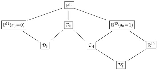
Figure 2. The inclusion diagram for the varieties of Dupin cyclides embedded in the spaces of Darboux cyclides.

The ideal in $\mathbb{R}[b_1,b_2,b_3,c_1,c_2,c_3,d_1,d_2,d_3,e_1,e_2,e_3,f_0]$ of the variety ${\mathcal{D}}_4$ is obtained from our main results on ${\mathcal{D}}_4^{*}$ by employing the normalizing shift (14). This shift transforms the general equation (1) for Darboux cyclides to

$$\begin{array}{cc}\hfill {\left(x^2+y^2+z^2\right)}^2& +\left(c_1-b_1^2-{\displaystyle \frac{B_0}{2}}\right)x^2+\left(c_2-b_2^2-{\displaystyle \frac{B_0}{2}}\right)y^2+\left(c_3-b_3^2-{\displaystyle \frac{B_0}{2}}\right)z^2\hfill \\ \hfill & +2(d_1-b_2{b}_3)yz+2(d_2-b_1{b}_3)xz+2(d_3-b_1{b}_2)xy\hfill \\ \hfill & +2\left(e_1+{\displaystyle \frac{b_1(B_0-c_1)-b_2{d}_3-b_3{d}_2}{2}}\right)x\hfill \\ \hfill & +2\left(e_2+{\displaystyle \frac{b_2(B_0-c_2)-b_1{d}_3-b_3{d}_1}{2}}\right)y\hfill \\ \hfill & +2\left(e_3+{\displaystyle \frac{b_3(B_0-c_3)-b_1{d}_2-b_2{d}_1}{2}}\right)z\hfill \\ \hfill & +f_0-{\displaystyle \frac{3B_0^2}{16}}+{\displaystyle \frac{W_3}{4}}-b_1{e}_1-b_2{e}_2-b_3{e}_3=0.\hfill \end{array}$$

(80)

Comparing the coefficients here with those in (15), we modify the equations for the variety ${\mathcal{D}}_4^{*}$ in Proposition 1 or Theorem 1, and obtain the defining equations for the space ${\mathcal{D}}_4$.

Moving towards ${\mathcal{D}}_3$ in Figure 2, the homogenized ideal for ${\mathcal{D}}_0$ is specified using the following standard result.

Proposition 2.

Let I be an ideal of the polynomial ring $k[x_1,\cdots ,x_n]$ over a field k, and let $\{g_1,\cdots ,g_t\}$ be a Gröbner basis for I with respect to a graded monomial ordering in $k[x_1,\cdots ,x_n]$. Denote by $f^h\in k[x_0,\cdots ,x_n]$ the homogenization of a polynomial $f\in k[x_1,\cdots ,x_n]$ with respect to the variable $x_0$. Then, $\{g_1^h,\cdots ,g_t^h\}$ is a Gröbner basis for the homogenized ideal $I^h=\left(f^h\mid f\in I\right)\subset k[x_0,\cdots ,x_n]$.

Proof. 

This is Theorem 4 in ([20], §8.4). □

We used Singular computations with respect to the total degree monomial ordering $grevlex(b_1,b_2,b_3,\dots ,f_0)$ ([20], p. 52). The computed that the Gröbner basis for ${\mathcal{D}}_0$ has 530 elements; the computation took about an hour on Singular. After the homogenization with $a_0$ and setting $a_0=0$, we obtain a reducible variety, where some components (possibly one) are restricted by $B_0=0$. We ignore these components by additionally assuming $B_0=1$. Then, the Gröbner basis with respect to $grevlex(b_1,b_2,b_3,\dots ,f_0)$ has 321 elements. The elimination of $e_1,e_2,e_3,f_0$ leads to the expressions of Theorem 2 with $B_0=1$, without any relation between the other coefficients of (19). This completes the alternative way of obtaining the ideal for ${\mathcal{D}}_3$.

Remark 4.

It is interesting to see what quadratic surfaces with $a_0=b_1=b_2=b_3=0$ in (1) are contained in the variety ${\mathcal{D}}_0$ as Dupin cyclides. After the substitution $a_0=b_1=b_2=b_3=0$ in the Gröbner basis with 530 elements, we obtain a reducible variety with two components of codimension 2 in ${\mathbb{P}}^9\subset {\mathbb{P}}^{13}$ (over $\mathbb{C}$). One component is defined by the vanishing of two polynomials: the discriminant of the characteristic polynomial of the matrix P in (36), and the determinant of this extended matrix:

$$\begin{array}{c}\hfill \widehat{P}=\left(\begin{array}{cccc}{c}_1& d_3& d_2& e_1\\ d_3& c_2& d_1& e_2\\ d_2& d_1& c_3& e_3\\ e_1& e_2& e_3& f_0\end{array}\right).\end{array}$$

(81)

The discriminant equals this sum of squares:

$$S_0^2+S_1^2+\left({\sigma }_{12}\right)S_1^2+{\left({\sigma }_{13}{S}_1\right)}^2+15T_1^2+15{\left({\sigma }_{12}{T}_1\right)}^2+15{\left({\sigma }_{13}{T}_1\right)}^2,$$

(82)

where

$$\begin{array}{cc}\hfill S_0& =(c_3-c_2)d_1^2+(c_1-c_3)d_2^2+(c_2-c_1)d_3^2+(c_1-c_2)(c_1-c_3)(c_2-c_3),\hfill \\ \hfill S_1& =d_1(d_2^2+d_3^2-2d_1^2)+(c_2+c_3-2c_1)d_2{d}_3+2(c_2-c_1)(c_3-c_1)d_1,\hfill \\ \hfill T_1& =d_1(d_2^2-d_3^2)+(c_2-c_3)d_2{d}_3.\hfill \end{array}$$

The real points of this component are therefore defined by the ideal generated by the three cubic polynomials $S_0,S_1,{\sigma }_{12}{S}_1,{\sigma }_{13}{S}_1,T_1,{\sigma }_{12}{T}_1,{\sigma }_{13}{T}_1$. This ideal defines a variety ${\mathcal{D}}_2$ of co-dimension 2. This variety is intersected with the degree four hypersurface $det\widehat{P}=0$ (which prescribes a singularity on the quadratic surface).

The second component restricts only the coefficients $c_1,c_2,c_3,d_1,d_2,d_3$ and coincides with ${\mathcal{D}}_2$. Hence, it subsumes the real points of the first component. The variety ${\mathcal{D}}_2$ specifies the quadratic part of (1) to be in the $O\left(3\right)$-orbit of $A_1{x}^2+A_1{y}^2+A_2{z}^2$. The projective dimension of this orbit is 3 (rather than $4=1+3$) because the rotations around the z-axis preserve $A_1{x}^2+A_1{y}^2+A_2{z}^2$. Based on the identification with ${\mathcal{D}}_2$, the rotational quadratic surfaces (and the paraboloids like $z^2+x=0$) can be considered as Dupin cyclides.

Remark 5.

We have seen from Theorem 2 that a cubic Dupin cyclide is determined uniquely from the coefficients $b_1,b_2,\cdots ,d_3$ to the cubic and quadratic monomials in (19). For quartic Dupin cyclides (1) with $a_0\ne 0$, the projection ${\mathcal{D}}_0\to {\mathbb{P}}^9$ to the coefficients $a_0,b_1,b_2,\cdots ,d_3$ is generically a 6:1 map. It is sufficient to see this 6:1 correspondence for the canonical form (23). With fixed $A_1,A_2,A_3$, there are these six possibilities for the linear part: $\pm Dx+F$, $\pm \left({\sigma }_{12}D\right)y+{\sigma }_{12}F$ and $\pm \left({\sigma }_{13}D\right)z+{\sigma }_{13}F$, with $D,F$ satisfying (24) and (25). It can also be checked (by computing a Gröbner basis) that a monomial basis for ${\mathcal{I}}_4^{*}$ in the ring $\mathbb{R}(c_1,c_2,c_3,d_1,d_2,d_3)[e_1,e_2,e_3,f_0]$ has six elements.

5.2. Dimension, Degree, Hilbert Series

It is straightforward to compute the Hilbert series for the computed ideals using Singular or Maple. The Hilbert series for the projective variety ${\mathcal{D}}_0$ is the rational function $H_1\left(t\right)/{(1-t)}^{10}$ with

$$\begin{array}{cc}\hfill H_1\left(t\right)=& 1+4t+10t^2+20t^3+35t^4+46t^5+39t^6+10t^7-14t^8-48t^9\hfill \\ \hfill & +25t^{10}+56t^{11}-105t^{12}+84t^{13}-37t^{14}+9t^{15}-t^{16}.\hfill \end{array}$$

(83)

The dimension of ${\mathcal{D}}_0$ is indeed $10-1=9$, and the degree equals $H_1\left(1\right)=134$. There are $\left({\displaystyle \genfrac{}{}{0pt}{}{8}{3}}\right)-46=10$ linearly independent polynomials of the minimal degree 5.

The Hilbert series for the affine variety ${\mathcal{D}}_4^{*}$ is

$$\begin{array}{c}\hfill {\displaystyle \frac{(1+t)(1+t+t^2)(1+2t+4t^2+t^3-t^4)}{{(1-t)}^6}}.\end{array}$$

(84)

The dimension of ${\mathcal{D}}_4^{*}$ is 6, and the degree equals 42.

The Hilbert series for projective variety ${\mathcal{D}}_3$ is

$$\begin{array}{c}\hfill {\displaystyle \frac{1+4t+10t^2+20t^3+35t^4-25t^5-9t^6+10t^7}{{(1-t)}^9}}.\end{array}$$

(85)

The dimension of ${\mathcal{D}}_3$ is $9-1=8$, and the degree equals 46. Recall that ${\mathcal{D}}_3$ describes the component $B_0\ne 0$ of the subvariety $a_0=0$ of ${\mathcal{D}}_0$. The homogeneous version of the Gröbner basis for ${\mathcal{D}}_3$ with respect to $grevlex(b_1,b_2,b_3,\dots ,f_0)$ has 261 elements. It has $\left({\displaystyle \genfrac{}{}{0pt}{}{8}{3}}\right)+25=81$ linearly independent polynomials of the minimal degree 5.

The co-dimension of all considered spaces of Dupin cyclides inside the corresponding projective spaces of Darboux cyclides equals 4.

Remark 6.

Besides the usual grading, the equations of our varieties have a weighted degree that reflects their invariance under the scaling $(x,y,z)\mapsto (\lambda x,\lambda y,\lambda z)$ with $\lambda \in \mathbb{R}$. The weights of the variables are the following:

$$wd\left(b_j\right)=1,wd\left(c_j\right)=wd\left(d_j\right)=2,wd\left(e_j\right)=3forj\in \{1,2,3\},$$

and $wd\left(a_0\right)=0$, $wd\left(f_0\right)=4$. The symmetries ${\sigma }_{12},{\sigma }_{13}$ do not change the weighted degree. The 12 equations in Proposition 1 have these weighted degrees:

$$wd\left(K_j\right)=8,wd\left(L_j\right)=7,wd\left(M_j\right)=9forj\in \{1,2,3\},$$

and $wd\left(N_1\right)=8$, $wd\left(N_2\right)=10$, $wd\left(N_3\right)=12$.

6. Classification of Real Cases of Dupin Cyclides

The torus equation (18) is also defined over $\mathbb{R}$ when $r^2<0$ or $R^2<0$. Similarly, the canonical equation (2) is defined over $\mathbb{R}$ if $\alpha ,\beta ,\gamma \in \mathbb{R}$, or if exactly two of these numbers are on the imaginary line, $\sqrt{-1}\mathbb{R}\subset \mathbb{C}$. Then, we may obtain degenerations to surfaces with a few (if any) real points.

Section 6.3 classifies all degenerations of Dupin cyclides. For that purpose, Section 6.1 defines general Möbius isomorphisms between Dupin cyclides and toruses and follows the cases when they are defined over $\mathbb{R}$. Section 6.2 defines a Möbius invariant $J_0$ of Dupin cyclides. This invariant and a few semi-algebraic conditions classify the Dupin cyclides up to real Möbius transformations.

6.1. Möbius Isomorphisms of the Torus

Spherical inversions or Möbius transformations between Dupin cyclides and a general torus have been constructed geometrically ([18], Theorem 3.5) and computed ([21], §2.3). An explicit Möbius isomorphism that maps a canonical Dupin cyclide (2) to the torus equation (18) is given by

$$\begin{array}{cc}\hfill (x,y,z)\mapsto & {\displaystyle \frac{\alpha \delta +\beta \epsilon }{\gamma }}(1,0,0)+{\displaystyle \frac{2\beta \epsilon }{{(x-\gamma )}^2+y^2+z^2}}(x-\gamma ,y,z),\hfill \end{array}$$

(86)

where $\beta =\sqrt{{\alpha }^2-{\gamma }^2}$, $\epsilon =\sqrt{{\delta }^2-{\gamma }^2}$. This Möbius transformation is defined over $\mathbb{R}$ if and only if $\gamma \in \mathbb{R}\setminus \left\{0\right\}$ and $\beta \epsilon \in \mathbb{R}$. If $\gamma =0$, the canonical equation (2) coincides already with the torus equation (18) with $\alpha =R$, $\delta =r$. With $\beta \epsilon \in \mathbb{R}$, the minor and major radii of the torus are given by

$$r={\displaystyle \frac{{\gamma }^2\epsilon }{\alpha \epsilon +\beta \delta }},R={\displaystyle \frac{{\gamma }^2\beta }{\alpha \epsilon +\beta \delta }},$$

(87)

We can further apply scaling by the factor

$${\displaystyle \frac{{\gamma }^2}{\alpha \epsilon +\beta \delta }}$$

(88)

to the immediate torus equation if either all $\alpha ,\delta ,\beta ,\epsilon \in \mathbb{R}$ or all $\alpha ,\delta ,\beta ,\epsilon \in \sqrt{-1}\mathbb{R}$. The resulting torus equation has $r=\epsilon$, $R=\beta$. Otherwise, the scaling can be adjusted by the factor $\sqrt{-1}$, and the radii become $r^2={\gamma }^2-{\delta }^2$, $R^2={\gamma }^2-{\alpha }^2$.

On the other hand, the canonical equation (2) is symmetrical ([6], (1)–(2)) with respect to the simultaneous interchange $y\leftrightarrow z$, $\alpha \leftrightarrow \gamma$. This symmetry implies a Möbius equivalence to the torus with the minor radius $\sqrt{R^2-r^2}$ (and the same major radius R) as well. Up to scaling, this Möbius equivalence is symmetric to (86):

$$\begin{array}{cc}\hfill (x,y,z)\mapsto & {\displaystyle \frac{\gamma \delta +\sqrt{({\gamma }^2-{\alpha }^2)({\delta }^2-{\alpha }^2)}}{\alpha }}(1,0,0)\hfill \\ \hfill & +{\displaystyle \frac{2\sqrt{({\gamma }^2-{\alpha }^2)({\delta }^2-{\alpha }^2)}}{{(x-\alpha )}^2+y^2+z^2}}(x-\alpha ,z,y),\hfill \end{array}$$

(89)

Both Möbius isomorphisms are defined over $\mathbb{R}$ if $\alpha \gamma \ne 0$ and ${\delta }^2$ is between ${\alpha }^2$ and ${\gamma }^2$ on the real line. This means that $0<r/R<1$ because (87) implies

$${\displaystyle \frac{r}{R}}=\sqrt{{\displaystyle \frac{{\delta }^2-{\gamma }^2}{{\alpha }^2-{\gamma }^2}}}.$$

(90)

A composition of the two Möbius isomorphisms relates two toruses with the minor radii r and $\sqrt{R^2-r^2}$, when $r<R$. This transformation is obtained explicitly by applying (89) with $\alpha =R$, $\gamma =0$, $\delta =r$. After additional scaling of $(x,y,z)$ by $r/R$, we obtain the Möbius transformation

$$\begin{array}{cc}\hfill (x,y,z)\mapsto & \left(\sqrt{R^2-r^2},0,0\right)+{\displaystyle \frac{2r\sqrt{R^2-r^2}}{{(x-r)}^2+y^2+z^2}}(x-r,z,y),\hfill \end{array}$$

(91)

that brings torus (18) to the torus

$${(x^2+y^2+z^2+r^2)}^2-4R^2(x^2+y^2)=0.$$

(92)

When $r^2{R}^2$, this Möbius duality is not defined over $\mathbb{R}$. If $0<R^2<r^2$, then (18) defines a singular spindle torus ([17], p. 288), and the surface (92) has no real points. If $0<R^2=r^2$, then (18) defines a singular horn torus, while (92) defines a circle.

6.2. The Toroidic Invariant for $r/R$

Any torus (18) has two clear families of circles on it, namely on the vertical planes $ax+by=0$ or horizontal planes $z=c$. These circles are the principal curvature lines on the torus and are known as principal circles. Less known are two families of Villarceau circles [22,23] on the bitangent planes $z=ax+by$ with $a^2+b^2=r^2/(R^2-r^2)$ on smooth toruses with $r<R$. The angles $\theta$, ${\displaystyle \frac{\pi }{2}}-\theta$ between principal and Villarceau circles depend only on the families of the involved circles. The sine (or the complementary cosine) of $\theta$ equals [23] the quotient $r/R$. The duality (91) of toruses with the minor radii r and $\sqrt{R^2-r^2}$ underscores constancy of the angle pair $\theta$, ${\displaystyle \frac{\pi }{2}}-\theta$ under the (conformal!) Möbius transformations. Krasauskas showed us that the numbers $r^2/R^2$ and $1-r^2/R^2$ are equal to the two possible cross-ratios within the quaternionic representation [11] of Dupin cyclides.

The symmetry between $r/R$ and $\sqrt{1-r^2/R^2}$ leads to this invariant under the Möbius transformations:

$$J_0={\displaystyle \frac{r^2}{R^2}}\left(1-{\displaystyle \frac{r^2}{R^2}}\right).$$

(93)

We define the invariant $J_0$ for general Dupin cyclides by the Möbius equivalence. The maximal value $J_0=1/4$ gives the “most round” cyclides (with $R=\sqrt{2}r$) that optimize the Willmore energy [24]

$$\int {\int }_S{H}^{2}dA$$

(94)

for the smooth real surfaces S with the torus topology. The integrand $H^2$ is the mean curvature H squared, and $dA$ is the infinitesimal area element. The Willmore energy is conformally invariant, and it equals ([25], p. 275)

$${\displaystyle \frac{{\pi }^2{R}^2}{r\sqrt{R^2-r^2}}}={\displaystyle \frac{{\pi }^2}{\sqrt{J_0}}}$$

(95)

for a smooth torus (18). The duality breaks down for $J_{0}0$, as Möbius transformation (91) is then not defined over $\mathbb{R}$. The singular-horn torus (with $r=R$) is paired to the degeneration to a circle ($r=0$), and the spindle toruses (with $r>R$) are paired with algebraic surfaces with no real points ($r\in \sqrt{-1}\mathbb{R}$).

We apply our results to compute the invariant $J_0$ for all Dupin cyclides. In the case of a canonical quartic cyclide (23), we choose Möbius equivalence (86) with a torus and obtain

$$\begin{array}{c}\hfill {\displaystyle \frac{r^2}{R^2}}={\displaystyle \frac{{\delta }^2-{\gamma }^2}{{\alpha }^2-{\gamma }^2}}={\displaystyle \frac{2A_2+A_3-A_1}{A_2-A_3}}\end{array}$$

(96)

due to (90) and (27). Then,

$$\begin{array}{cc}\hfill J_0& =-{\displaystyle \frac{({\delta }^2-{\gamma }^2)({\delta }^2-{\alpha }^2)}{{({\alpha }^2-{\gamma }^2)}^2}}\hfill \end{array}$$

(97)

$$\begin{array}{cc}\hfill & ={\displaystyle \frac{(A_1-2A_2-A_3)(A_2+2A_3-A_1)}{{(A_2-A_3)}^2}}.\hfill \end{array}$$

(98)

To obtain expressions of $J_0$ for the general quartic cyclide (15), we first eliminate $A_2,A_3$ as in Lemma 3. The result is

$$\begin{array}{c}\hfill J_0={\displaystyle \frac{7A_1^2-8C_0{A}_1+2C_0^2+W_1}{3A_1^2-2C_0{A}_1-C_0^2+4W_1}}.\end{array}$$

(99)

After the elimination of $A_1$, we generically obtain

$$\begin{array}{cc}\hfill J_0& ={\displaystyle \frac{6C_0(d_2{e}_1+d_1{e}_2-c_1{e}_3-c_2{e}_3)+(C_0^2+8W_1+28f_0)e_3}{4C_0(d_2{e}_1+d_1{e}_2-c_1{e}_3-c_2{e}_3)+(7W_1+12f_0)e_3}}\hfill \end{array}$$

(100)

$$\begin{array}{cc}\hfill & ={\displaystyle \frac{(4f_0-C_0^2)(28f_0+C_0^2)+4(8f_0+C_0^2)W_1-12C_0(W_2-2E_0)}{12f_0(4f_0-C_0^2)+(28f_0+C_0^2)W_1-8C_0(W_2-2E_0)}}.\hfill \end{array}$$

(101)

These expressions were obtained after heavy Gröbner basis computations with the new variable $J_0$ (or rather, its numerator and denominator separately) and the superfluous $A_1$. They can be checked by reducing (to 0) the numerator of the difference to (99) in the Gröbner basis in ${\mathcal{R}}_4^{*}\left[A_1\right]$ for Lemma 3.

To obtain an expression of $J_0$ for the cubic cyclide (3), we apply the procedure at the beginning of this section: transform the variables according to the shift (14) and the form (1), homogenize with $a_0$, and set $a_0=0$. Here is a relatively compact rational expression of the lowest weighted degree obtained after heavy computations:

$$J_0=3{\displaystyle \frac{B_0(-2Y_5+c_1{c}_2+c_1{c}_3+c_2{c}_3)+Y_6}{B_0(Y_5+2c_1^2+2c_2^2+2c_3^2+c_1{c}_2+c_1{c}_3+c_2{c}_3)+2Y_6}},$$

(102)

with $Y_5=d_1^2+d_2^2+d_3^2-4b_1{e}_1-4b_2{e}_2-4b_3{e}_3$, and

$$\begin{array}{cc}\hfill Y_6=& 5b_1^2{d}_1^2+5b_2^2{d}_2^2+5b_3^2{d}_3^2+10b_1{b}_2(c_3{d}_3-d_1{d}_2)+10b_1{b}_3(c_2{d}_2-d_1{d}_3)\hfill \\ \hfill & +10b_2{b}_3(c_1{d}_1-d_2{d}_3)-2C_0(b_1{b}_2{d}_3+b_1{b}_3{d}_2+b_2{b}_3{d}_1)\hfill \\ \hfill & -b_1^2(c_1^2+4c_2{c}_3)-b_2^2(c_2^2+4c_1{c}_3)-b_3^2(c_3^2+4c_1{c}_2).\hfill \end{array}$$

The variables $e_1,e_2,e_3$ could be eliminated in (102) using Lemma 2, but the obtained rational expression of degree 6 (after using $B_0=1$) is much larger.

6.3. Classification of Degenerate Dupin Cyclides

The cubic Dupin cyclides (3) always have real points and are easy to classify, starting from ([7], p. 151), ([17], p. 288):

• Smooth cyclides when $pq<0$;
• Spindle cyclides when $pq>0$, $p\ne q$;
• Horn cyclides when $pq=0$, $p\ne q$;
• Reducible surface (a sphere and a tangent plane) when $p=q\ne 0$;
• Reducible surface (a plane and a point on it) when $p=q=0$.

Degeneration to quadratic surfaces is explained in Remark 4.

The full classification of the real points defined by the quartic canonical equation (2) depends on the order of $0,{\alpha }^2,{\gamma }^2,{\delta }^2$ on the real line, as we demonstrate briefly. The classification is depicted in Figure 3a. The border conditions ${\alpha }^2=0$, ${\gamma }^2=0$, ${\delta }^2=0$ are depicted by three intersecting circles (marked on the outer side by ${\alpha }^2,{\gamma }^2,{\delta }^2$). Their inside disks represent positive values of ${\alpha }^2,{\gamma }^2,{\delta }^2$, respectively, while the negative values are represented by the outer sides of the circles. The conditions ${\alpha }^2={\gamma }^2,{\alpha }^2={\delta }^2,{\gamma }^2={\delta }^2$ are represented by the three lines intersecting at the center. Their markings near the edge of the picture (say, ${\alpha }^2$ and ${\gamma }^2$) indicate which of the values (${\alpha }^2$ or ${\gamma }^2$) is larger on either side of the line. Most triangular regions are marked by a sequence of inequalities between $0,{\alpha }^2,{\gamma }^2,{\delta }^2$; these admissible regions represent the cases when the canonical equation is defined over $\mathbb{R}$. The six asymptotic outside regions represent the cases when all three ${\alpha }^2,{\gamma }^2,{\delta }^2$ are negative; they are not admissible. The admissible regions, several edges, and vertices are labeled by abbreviations for various types of Dupin cyclides. The labels are not repeated when the type does not change when passing from a triangular region to its edge or vertex. These coincidences are represented by the non-strict inequalities between 0 and ${\alpha }^2,{\gamma }^2,{\delta }^2$. When a distinct edge and its vertex have the same type, the type is indicated near the vertex, and an arrow is added to the direction of that edge. The values of $J_0$ can be considered as constant along the radial directions from the center Q, with the optimal $J_0=1/4$ in the vertical directions, $J_0=-\infty$ on the horizontal line ${\alpha }^2={\gamma }^2$, and $J_0=0$ along the other two drawn lines; see (97). The trivial case $({\alpha }^2,{\gamma }^2,{\delta }^2)=(0,0,0)$ is not represented in Figure 3a, though it is represented by the origin point in Figure 3b.

Figure 3. (a) Classification of real points on quartic cyclides in the canonical form (2). (b) Classification of real points on toruses (18). (c) Legend.

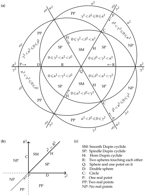
This classification can be proved from the easier classification of torus equations (18) in Figure 3b, and by considering which of the two Möbius transformations (86) and (89) are defined over $\mathbb{R}$. The case $r^2<min(0,R^2)$ of “toruses” with no real points can be seen from this alternative form of (18):

$${(x^2+y^2+z^2-R^2+r^2)}^2-4r^2(x^2+y^2)+4(R^2-r^2)z^2=0.$$

(103)

The cases of toruses lie on the circles ${\gamma }^2=0$ and ${\alpha }^2=0$ of Figure 3a. The Möbius equivalence (86) is defined over $\mathbb{R}$ if ${\gamma }^2>0$ and ${\gamma }^2$ is either larger or smaller than both ${\alpha }^2,{\delta }^2$. It preserves $J_0$ and maps the applicable triangular regions onto the segments of the circle ${\gamma }^2=0$ representing toruses. The adjacency of the corresponding triangular regions and segments cannot hold for the two lower-right regions SM, SP with ${\alpha }^2,{\delta }^2\in [0,{\gamma }^2)$; these are the cases when the scaling by (88) has to be adjusted by $\sqrt{-1}$. Similarly, (89) is defined over $\mathbb{R}$ if ${\alpha }^2>0$ and ${\alpha }^2$ is either larger or smaller than both ${\gamma }^2,{\delta }^2$. This covers all cases except the line ${\alpha }^2={\gamma }^2$ and the two leftmost triangular regions. When ${\alpha }^2={\gamma }^2$, the canonical equation (2) factorizes and defines (generically) two spheres with the centers at $(x,y,z)=(\pm \alpha ,0,0)$ and touching at the point $(\delta ,0,0)$. If, then, ${\alpha }^2<0$, only the touching point is real; the other few deeper degenerations are straightforward. For the leftmost triangular region with ${\gamma }^2<{\alpha }^2⩽0$, the canonical equation can be rearranged to

$${\left(x^2+y^2+z^2-{\alpha }^2+{\gamma }^2-{\delta }^2\right)}^2+4(-{\gamma }^2+{\alpha }^2)z^2+(-4){(\alpha \delta -\gamma x)}^2=0;$$

(104)

see ([19], p. 325). All three terms are positive for that region, and the Dupin surface then consists of two points on the line $z=0$, $x=\alpha \delta /\gamma$. Similarly, two points are obtained for the other leftmost region ${\alpha }^2<{\gamma }^2⩽0$.

The SM-regions for smooth Dupin cyclides separate pairs of SP-regions for spindle cyclides. Accordingly, there are two types of spindle cyclides in ${\mathbb{R}}^3$; see Figure 4(a,b) or ([18], Fig. 3), ([21], Fig. 2.23). Spindle cyclides have two real singular points that either (a) delimit a lemon-shaped volume inside an apple-shaped body [26] confined by the self-intersecting surface, or (b) delimit two horn-shaped volumes. These two types of spindle cyclides are related by a spherical inversion centered inside the apple or horn parts. There are two types of horn cyclides as well; see Figure 4(c,d). They are the limiting cases of the two types of spindles cyclides, with one real singular point.

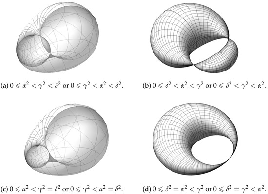
Figure 4. (a,b) Spindle Dupin cyclides. (c,d) Horn Dupin cyclides.

The conditions on ${\alpha }^2,{\gamma }^2,{\delta }^2$ can be directly translated to the conditions on the coefficients $A_1,A_2,A_3$ in (23) using (27). The quadratic covering (24) of the $(A_1,A_2,A_3)$-plane confirms the topology of four admissible regions connected at six corners. The translated classification is as follows:

• Smooth Dupin cyclides, when $A_1⩽min(A_2,A_3)<A_1-A_2-A_3<max(A_2,A_3)$. Then $J_0\in (0,{\displaystyle \frac{1}{4}}]$ and $A_2\ne A_3$, $A_2+A_3<0$.
• Spindle cyclides, when either (a) $A_1⩽min(A_2,A_3)<max(A_2,A_3)<A_1-A_2-A_3$. or (b) $A_1-min(A_2,A_3)<A_2+A_3⩽0$, $A_2\ne A_3$, with reference to Figure 4. In either case, $J_0<0$, $A_2\ne A_3$.
• Horn cyclides, when either (c) $A_1-A_2-A_3=max(A_2,A_3)<0$, $A_2\ne A_3$, or (d) $A_1-min(A_2,A_3)=A_2+A_3<0$, $A_2\ne A_3$. In either case, $J_0=0$.
• The reducible surface of two touching spheres, when $3A_2<A_1<A_2=A_3$ (then $A_2=A_3<0$) or $A_1<A_2=A_3⩽0$. In either case, $J_0=-\infty$.
• Reducible surface of a sphere and a point on it, when $A_2=A_3={\displaystyle \frac{1}{3}}{A}_1<0$. Then, $J_0$ is undefined.
• Double sphere, when $A_1=A_2=A_3<0$. Then $J_0=-\infty$.
• A circle, when $A_2+A_3=0$, $A_1=min(A_2,A_3)<0$. Then $J_0=0$, $A_1<0$.
• Two real points, when either $min(A_2,A_3)<A_1-A_2-A_3⩽A_1⩽max(A_2,A_3)$ (then $J_0>0$, $A_2\ne A_3$, $A_2+A_3⩾0$) or $max(A_2,A_3)⩽A_1⩽A_1-A_2-A_3$, $A_2\ne A_3$ (then $J_0<0$, $A_2+A_3⩽0$).
• One real point, when either $A_1-A_2-A_3=min(A_2,A_3)⩽0$, $A_2+A_3>0$ (then $J_0=0$), or $0⩽A_2=A_3<A_1$ (then $J_0=-\infty$), or $A_1=A_2=A_3=0$.
• No real points, when $A_1-A_2-A_3<min(A_2,A_3)⩽A_1⩽max(A_2,A_3)$. Then $J_0<0$, $A_2+A_3>0$.

Further translation in terms of the coefficients in (15) is cumbersome. Some basic distinctions are determined by the $J_0$-invariant, represented by the directions from the central point Q in Figure 3a. The circular boundaries ${\alpha }^2=0$, ${\gamma }^2=0$, ${\delta }^2=0$ do not represent semi-algebraic conditions (except at the vertices C, D), as they separate the cases of whether the surface equations (2) and eventually (15), (1) are defined over $\mathbb{R}$ or not. To distinguish the six regions around Q and the six outer regions, it is tempting to invent a polynomial that vanishes at the vertices C and D and has different signs for the inner and outer regions. But the polynomials in ${\alpha }^2,{\gamma }^2,{\delta }^2$ (or the other coefficients) that vanish at C and D also vanish at the opposite meeting corners or the PP and NP regions. The practical suggestion to distinguish the cases is to compute $A_1$ using one of the equations (linear in $A_1$) of Lemma 3, and then compute $A_2,A_3$ as the roots of the quadratic polynomial $X^2-(A_2+A_3)X+A_2{A}_3$. After eliminating $A_2,A_3$, we obtain the equation

$$X^2+(A_1-C_0)X+W_1-C_0{A}_1+A_1^2=0$$

(105)

with the roots $X=A_2$, $X=A_3$. If preferable, one can reduce the degree in $A_1$ in the last equation using (43).

7. Conclusions

Dupin cyclides are algebraic surfaces in the 3-dimensional Euclidean space, of degree four or three, that have applications in geometric design and architecture. The larger class of Darboux cyclides is promising for these applications as well, yet recognising Dupin cyclides from the implicit equation (1) will remain an important practical problem. Considering the free coefficients in (1) as projective coordinates, we identify the space of Darboux cyclides as the projective space ${\mathbb{P}}^{13}$. The points in ${\mathbb{P}}^{13}$ that correspond to Dupin cyclides form an algebraic variety ${\mathcal{D}}_0$ of codimension 4. It can be computed as the orbit of canonical equations (2) and (3) under Euclidean transformations in ${\mathbb{R}}^3$. This article aims at establishing practical sets of algebraic equations for ${\mathcal{D}}_0$ or its representative subvarieties. Additionally, Section 6.3 classifies the real types of Dupin cyclides and their degenerations.

The affine chart ${\mathbb{R}}^{13}\subset {\mathbb{P}}^{13}$ represents quartic Darboux cyclides. The affine variety ${\mathcal{D}}_4$ of quartic Dupin cyclides can be simplified by affine translations (14) to the representative variety ${\mathcal{D}}_4^{*}$ of Section 3; see Figure 2. The equations for ${\mathcal{D}}_4^{*}$ are formulated in Proposition 1 and Theorem 1. The latter theorem is more practical as it specifies the minimal number (the codimension 4) of equations to check, depending on a convenient stratification of ${\mathbb{P}}^{13}$. This stratifies ${\mathcal{D}}_4^{*}$ locally into complete intersections. The cubic cyclides are located at infinity of ${\mathbb{P}}^{13}$, and the equations defining the cubic (also known as parabolic) Dupin cyclides are formulated in Theorem 2. The variety ${\mathcal{D}}_3$ of cubic Dupin cyclides is a complete intersection already. It contains the Zariski closure of ${\mathcal{D}}_4$ in ${\mathbb{P}}^{13}$, as pointed out in Section 5. The requisite extensive computations with Gröbner bases were carried out using the computer algebra systems Maple 2018 and Singular 4.2.1.

An algorithm for recognizing Dupin cyclides based on the results of this article is implemented in Maple. It is available at https://github.com/menjanahary/DupinRecognitionAlgorithm (accessed on 29 July 2024). We checked the efficiency of this implementation on a five-parameter family of cyclide equations constructed following the classical definition [12,17,27] of Dupin cyclides as the envelope of a one-parameter family of spheres touching three fixed spheres. Let us specify a sphere $S(c,r)$ by its center c and the radius r. The tangential distance between two spheres $S_1(c_1,r_1)$ and $S_2(c_2,r_2)$ equals $|S_1-S_2|=\sqrt{|c_1-c_2{|}^2-{(r_1-r_2)}^2}$. Up to Euclidean transformations and scaling, we can assume that the three fixed spheres generating a Dupin cyclide are given by $S_0((0,0,0),1)$, $S_1((a_1,0,0),r_1)$, $S_2((a_2,a_3,0),r_2)$. Following Darboux [28], a point X on the Dupin cyclide is treated as a sphere with a radius of zero. The Dupin cylide defined by $S_0,S_1,S_2$ satisfies the equation

$${(t_1^2{d}_{02}^2+t_2^2{d}_{01}^2-t_0^2{d}_{12}^2)}^2-4{\left(t_1{t}_2{d}_{01}{d}_{02}\right)}^2=0,$$

(106)

where $d_{ij}=|S_i-S_j|$ and $t_i=|X-S_i|$. Using the localized formulation in Theorem 1, the Maple implementation took about 136 s CPU time (on AMD Ryzen 5 4500U processor running at 2.38 GHz) to decide that this equation indeed defines a Dupin cyclide generally. The large defining equations of Proposition 1 could not be checked within a reasonable time for this particular example.

The main results of this article were used recently [29] for deriving algebraic conditions for blending Dupin cyclides along a fixed circle. An important problem for future work is to understand the geometric meaning of linear subspaces within the variety of Dupin cyclides. For instance, some lines in this variety represent Dupin cyclides that blend smoothly along a Villarceau circle ([29], § 6.2). Another research direction is to determine the number of non-degenerate Dupin cyclides that a line in ${\mathbb{P}}^{13}$ can contain. This problem is related to the task of fitting nine generic points with Dupin cyclides. This will enhance our understanding of the capacity of Dupin cyclides in geometric fitting problems. The problem of fitting cones, cylinders, and toruses through a set of points is solved already in [30,31].

References

- Darboux, G. Principes de Géométrie Analytique; Gauthier-Villars: Paris, France, 1917. [Google Scholar]
- Pottmann, H.; Shi, L.; Skopenkov, M. Darboux cyclides and webs from circles. Comput. Aided Geom. Des. 2012, 29, 77–97. [Google Scholar] [CrossRef][Green Version]
- Krasauskas, R.; Zube, S. Kinematic interpretation of Darboux cyclides. Comput. Aided Geom. Des. 2020, 83, 101945. [Google Scholar] [CrossRef]
- Zhao, M.; Jia, X.; Tu, C.; Mourrain, B.; Wang, W. Enumerating the morphologies of non-degenerate Darboux cyclides. Comput. Aided Geom. Des. 2019, 75, 101776. [Google Scholar] [CrossRef]
- Martin, R.R. Principal patches—A new class of surface patch based on differential geometry. In Eurographics’83; Ten Hagen, P.J.W., Ed.; North-Holland: Amsterdam, The Netherlands, 1983; pp. 47–55. [Google Scholar]
- Pratt, M.J. Cyclides in computer aided geometric design. Comput. Aided Geom. Des. 1990, 7, 221–242. [Google Scholar] [CrossRef]
- Pratt, M.J. Cyclides in computer aided geometric design II. Comput. Aided Geom. Des. 1995, 12, 131–152. [Google Scholar] [CrossRef]
- Druoton, L.; Langevin, R.; Garnier, L. Blending canal surfaces along given circles using Dupin cyclides. Int. J. Comput. Math. 2014, 91, 641–660. [Google Scholar] [CrossRef]
- Allen, S.; Dutta, D. Cyclides in pure blending I. Comput. Aided Geom. Des. 1997, 14, 51–75. [Google Scholar] [CrossRef]
- Allen, S.; Dutta, D. Cyclides in pure blending II. Comput. Aided Geom. Des. 1997, 14, 77–102. [Google Scholar] [CrossRef]
- Zube, S.; Krasauskas, R. Representation of Dupin cyclides using quaternions. Graph. Models 2015, 82, 110–122. [Google Scholar] [CrossRef]
- Krasauskas, R.; Mäurer, C. Studying cyclides with Laguerre geometry. Comput. Aided Geom. Des. 2000, 17, 101–126. [Google Scholar] [CrossRef]
- Peternell, M.; Pottmann, H. A Laguerre geometric approach to rational offsets. Comput. Aided Geom. Des. 1998, 15, 223–249. [Google Scholar] [CrossRef]
- Blum, R. Circles on surfaces in the Euclidean 3-space. In Geometry and Differential Geometry; Artzy, R., Vaisman, I., Eds.; Lecture Notes in Mathematics; Springer: Berlin/Heidelberg, Germany, 1980; pp. 213–221. [Google Scholar]
- Takeuchi, N. Cyclides. Hokkaido Math. J. 2000, 29, 119–148. [Google Scholar] [CrossRef]
- Bastl, B.; Jüttler, B.; Lávička, M.; Schulz, T.; Šír, Z. On the parameterization of rational ringed surfaces and rational canal surfaces. Math. Comput. Sci. 2014, 8, 299–319. [Google Scholar] [CrossRef]
- Chandru, V.; Dutta, D.; Hoffmann, C.M. On the geometry of Dupin cyclides. Vis. Comput. 1989, 5, 277–290. [Google Scholar] [CrossRef]
- Ottens, L. Dupin Cyclides. Bachelor’s Thesis, Faculty of Science and Engineering, University of Groningen, Groningen, The Netherlands, 2012. [Google Scholar]
- Forsyth, A. Lectures on the Differential Geometry of Curves and Surfaces; Cambridge University Press: Cambridge, UK, 1912. [Google Scholar]
- Cox, D.; Little, J.; O’Shea, D.; Sweedler, M. Ideals, Varieties, and Algorithms; Springer: New York, NY, USA, 1997; Volume 3. [Google Scholar]
- van der Valk, M. On Dupin Cyclides. Bachelor’s Thesis, Faculty of Science and Engineering, University of Groningen, Groningen, The Netherlands, 2009. [Google Scholar]
- Yvon Villarceau, A.J. Extrait d’une note communiquée à M. Babinet par M. Yvon Villarceau. C. R. Hebd. Séances l’Acad. Sci. 1848, 27, 246. [Google Scholar]
- Weisstein, E.W. Villarceau Circles. 2008. Available online: https://mathworld.wolfram.com/VillarceauCircles.html (accessed on 29 July 2024).
- White, J.H. A global invariant of conformal mappings in space. Proc. Am. Math. Soc. 1973, 38, 162–164. [Google Scholar] [CrossRef]
- Willmore, T.J. Riemannian Geometry; Oxford University Press: Oxford, UK, 1993. [Google Scholar]
- Rigaud, G.; Hahn, B. Reconstruction algorithm for 3D Compton scattering imaging with incomplete data. Inverse Probl. Sci. Eng. 2020, 29, 967–989. [Google Scholar] [CrossRef]
- Dupin, C. Applications de Géométrie et de Méchanique; Bachelier: Paris, France, 1822. [Google Scholar]
- Darboux, G. Sur les sections du tore. Nouvelles Ann. Math. 1864, 3, 156–165. [Google Scholar]
- Menjanahary, J.M.; Vidunas, R. Dupin cyclides passing through a fixed circle. Mathematics 2024, 12, 1505. [Google Scholar] [CrossRef]
- Buse, L.; Galligo, A.; Zhang, J. Extraction of cylinders and cones from minimal point sets. Graph. Models 2016, 86, 1–12. [Google Scholar] [CrossRef]
- Buse, L.; Galligo, A. Extraction of tori from minimal point sets. Comput. Aided Geom. Des. 2017, 58, 1–7. [Google Scholar] [CrossRef]
Disclaimer/Publisher’s Note: The statements, opinions and data contained in all publications are solely those of the individual author(s) and contributor(s) and not of MDPI and/or the editor(s). MDPI and/or the editor(s) disclaim responsibility for any injury to people or property resulting from any ideas, methods, instructions or products referred to in the content. |
© 2024 by the authors. Licensee MDPI, Basel, Switzerland. This article is an open access article distributed under the terms and conditions of the Creative Commons Attribution (CC BY) license (https://creativecommons.org/licenses/by/4.0/).