Dynamics of a Predator–Prey System with Impulsive Stocking Prey and Nonlinear Harvesting Predator at Different Moments

Abstract

In this article, we study a predator–prey system, which includes impulsive stocking prey and a nonlinear harvesting predator at different moments. Firstly, we derive a sufficient condition of the global asymptotical stability of the predator–extinction periodic solution utilizing the comparison theorem of the impulsive differential equations and the Floquet theory. Secondly, the condition, which is to maintain the permanence of the system, is derived. Finally, some numerical simulations are displayed to examine our theoretical results and research the effect of several important parameters for the investigated system, which shows that the period of the impulse control and impulsive perturbations of the stocking prey and nonlinear harvesting predator have a significant impact on the behavioral dynamics of the system. The results of this paper give a reliable tactical basis for actual biological resource management.

1. Introduction

The protection of biological diversity is a historic commitment by the world’s nations to employ biological resources sustainably [1]. Increasing human population and environmental pollution problems require humankind to devote more and more attention to the conservation of biological resources. There are many authors and papers studying biological resource management [1,2,3,4,5,6]. However, the protection of biological resources is not over for humans although it has been sustained for a long time.

In the real world, there are many relationships between species, for instance, competition, mutualism and predator–prey, which as an important role among them has been studied by many papers [7,8,9,10,11,12,13,14,15,16,17,18,19,20]. The authors of those papers considered all kinds of conditions on the prey, predator or entire model. For example, Xiao and Chen [7], and Chattopadhyay and Arino [8] studied a predator–prey model with disease in the prey; Georgescu and Hsieh [9] researched the dynamics of a predator–prey system with a stage structure; the above-mentioned authors do not study the impulsive differential equations in corresponding papers. However, it is preferable to introduce impulse into systems when we consider systems subjected to sudden changes such as fires, floods and so on [11]. In reference [11], Liu and Chen discussed the following predator–prey model with impulsive perturbation in the predator.

$$\left\{\begin{array}{c}\left.\begin{array}{c}{\displaystyle \frac{d{x}_1\left(t\right)}{dt}}=a{x}_1\left(t\right)-b{x}_1^2\left(t\right)-{\displaystyle \frac{\alpha x_1\left(t\right)x_2\left(t\right)}{1+\omega x_1\left(t\right)}},\hfill \\ {\displaystyle \frac{d{x}_2\left(t\right)}{dt}}={\displaystyle \frac{k\alpha x_1\left(t\right)x_2\left(t\right)}{1+\omega x_1\left(t\right)}}-c{x}_2\left(t\right),\hfill \end{array}\right\}t\ne n\gamma ,\hfill \\ \left.\begin{array}{c}{x}_1\left(n{\gamma }^{+}\right)=x_1\left(n\gamma \right),\hfill \\ x_2\left(n{\gamma }^{+}\right)=x_2\left(n\gamma \right)+p,\hfill \end{array}\right\}t=n\gamma ,\hfill \end{array}\right.$$

The biological meaning of the parameters of the model refer to [11]. With the application of impulsive perturbation in predator–prey systems, research on predator–prey systems is becoming more and more diverse. Reference [12] studied a prey–predator system with a stage structure about both prey and predator, and impulsive constant inputting predator and diseased prey. Reference [14] studied a state-dependent feedback control prey–predator system with anti-predator behavior. At the same time, predator–prey models and impulsive differential equations are also applied to control pests [15,20,21,22,23,24,25,26,27,28], which provides a reliable tactical basis for controlling pests in agriculture production, where prey and predator represent pests and natural enemies, respectively. We have listed only a few of the papers on the predator and prey models; in fact, it is not difficult to discover that the predator–prey relationship is a popular topic in population dynamics based on a review of previous papers [18].

Predator and prey models have been applied not only to pest management but also to the exploitation of ecological resources [16,17,18,19,29]; among them, reference [16] did not research impulsive harvesting and impulsive stocking, reference [18] contained the impulsive diffusing of prey and harvesting of both predator and prey, reference [19] considered the impulsive birth of the prey and harvesting of the predator, and reference [29] included the birth impulse of the prey and the impulsive harvesting of both prey and predator. In particular, Jiao [17] mentioned the following delayed differential equations with impulsive constant stocking prey.

$$\left\{\begin{array}{c}\left.\begin{array}{c}{x}^{\prime }\left(\gamma \right)=x\left(\gamma \right)(a_1-b_{1}x\left(\gamma \right))-{\displaystyle \frac{\beta x\left(\gamma \right)}{1+cx\left(\gamma \right)}}{x}_2\left(\gamma \right),\hfill \\ x_1^{\prime }\left(\gamma \right)=r_1{x}_1\left(\gamma \right)-r_1{e}^{-\omega {\tau }_1}{x}_2(\gamma -{\tau }_1)-\omega x_1\left(\gamma \right),\hfill \\ x_2^{\prime }\left(\gamma \right)=r_1{e}^{-\omega {\tau }_1}{x}_2(\gamma -{\tau }_1)+{\displaystyle \frac{k\beta x\left(\gamma \right)}{1+cx\left(\gamma \right)}}{x}_2\left(\gamma \right)-d_3{x}_2\left(\gamma \right)-E{x}_2\left(\gamma \right)-d_4{x}_2^2\left(\gamma \right),\hfill \end{array}\right\}\gamma \ne n\tau ,\hfill \\ \left.\begin{array}{c}\Delta x\left(\gamma \right)=m,\hfill \\ \Delta x_1\left(\gamma \right)=0,\hfill \\ \Delta x_2\left(\gamma \right)=0,\hfill \end{array}\right\}\gamma =n\tau ,n=1,2\dots ,\hfill \\ (\varphi \left(\eta \right),{\varphi }_1\left(\eta \right),{\varphi }_2\left(\eta \right))\in C_{+}=C([-{\tau }_1,0],R_{+}^3),\varphi \left(0\right)>0,{\varphi }_1\left(0\right)>0,{\varphi }_2\left(0\right)>0.\hfill \end{array}\right.$$

(1)

The specific biological significance of the parameters, which are concluded by system (1), are as follows. $x\left(\gamma \right),$ $x_1\left(\gamma \right)$ and $x_2\left(\gamma \right)$ are prey density, immature predator density and mature predator density, respectively. The intrinsic growth rate and the coefficient of intraspecific competition of the predator are $a_1>0$ and $b_1>0,$ respectively. $r_1>0$ is the birth rate of the immature predator. $\omega >d_3$ and $k>0$ are the ratio of converting prey into predator. $c>0$ is the shape parameter of the prey. $d_3>0$ and $d_4>0$ are death rate of the mature predator, which follows a logistic nature. Further, Jiao et al. [30] studied the next prey–predator model with impulsive harvesting in both prey and predator.

$$\left\{\begin{array}{c}\left.\begin{array}{c}{\displaystyle \frac{dx\left(v\right)}{dv}}=x\left(v\right)(a_1-b_{1}x\left(v\right))-{\beta }_{1}x\left(v\right)y\left(v\right),\hfill \\ {\displaystyle \frac{dy\left(v\right)}{dv}}=k_1{\beta }_{1}x\left(v\right)y\left(v\right)-d_{1}y\left(v\right),\hfill \end{array}\right\}v\in (n\gamma ,(n+\tau )\gamma ],\hfill \\ \left.\begin{array}{c}\Delta x\left(v\right)=-h_{0}x\left(v\right),\hfill \\ \Delta y\left(v\right)=0,\hfill \end{array}\right\}v=(n+\tau )\gamma ,n\in Z_{+},\hfill \\ \left.\begin{array}{c}{\displaystyle \frac{dx\left(v\right)}{dv}}=-d_{2}x\left(v\right)-{\beta }_{2}x\left(v\right)y\left(v\right),\hfill \\ {\displaystyle \frac{dy\left(v\right)}{dv}}=k_2{\beta }_{2}x\left(v\right)y\left(v\right)-d_{3}y\left(v\right),\hfill \end{array}\right\}v\in ((n+\tau )\gamma ,(n+1)\gamma ],\hfill \\ \left.\begin{array}{c}\Delta x\left(v\right)=0,\hfill \\ \Delta y\left(v\right)=-h_{1}y\left(v\right),\hfill \end{array}\right\}v=(n+1)\gamma ,n\in Z_{+},\hfill \end{array}\right.$$

$h_0,$ a positive constant expressing the harvesting ratio of the prey at time $v=(n+\tau )\gamma ,$ is less than 1. Similarly, $h_1,$ the harvesting ratio of the predator at $v=(n+1)\gamma ,$ is also less than 1 and more than 0. For the specific biological meaning of other parameters of the above model, refer to [30].

There are relatively few predator–prey models on impulsive releasing prey and impulsive nonlinear harvesting predators although there have been many studies on predator–prey systems [21,31,32]. We examine the next predator and prey model, which includes impulsive releasing prey and a nonlinear harvesting predator, for biological resource management in this article, for example, periodical stocking prey and harvesting predator, which has significant economic value, when people feed fish, soft-shelled turtle, crocodiles and so on. It is worth noting that here two impulses happen at different moments.

$$\left\{\begin{array}{c}\left.\begin{array}{c}{\displaystyle \frac{d{x}_0\left(v\right)}{dv}}=a_0{x}_0\left(v\right)(1-{\displaystyle \frac{x_0\left(v\right)}{K_1}})-{\displaystyle \frac{{\beta }_0{x}_0\left(v\right)y_0\left(v\right)}{1+{\alpha }_0{x}_0\left(v\right)}},\hfill \\ {\displaystyle \frac{d{y}_0\left(v\right)}{dv}}=-d_0{y}_0\left(v\right)+{\displaystyle \frac{k{\beta }_0{x}_0\left(v\right)y_0\left(v\right)}{1+{\alpha }_0{x}_0\left(v\right)}},\hfill \end{array}\right\}v\ne (n+\sigma )F,v\ne (n+1)F,\hfill \\ \left.\begin{array}{c}\Delta x_0\left(v\right)={\mu }_0,\hfill \\ \Delta y_0\left(v\right)=0,\hfill \end{array}\right\}v=(n+\sigma )F,\hfill \\ \left.\begin{array}{c}\Delta x_0\left(v\right)=0,\hfill \\ \Delta y_0\left(v\right)=-{\displaystyle \frac{h_{max}{y}_0\left(v\right)}{{\alpha }_1+y_0\left(v\right)}}{y}_0\left(v\right),\hfill \end{array}\right\}v=(n+1)F.\hfill \end{array}\right.$$

(2)

where $x_0\left(v\right)$ and $y_0\left(v\right)$ represent the population densities of prey and predator at time v, respectively. Parameter $F>0$ denotes the period of the impulse, $(n+\sigma )F(0<\sigma <1)$ is the first impulsive time and $n\ge 0$ denotes the impulse amounts. $K_1,$ a positive constant, is the maximum environmental capacity. $a_0>0$ denotes the intrinsic growth rate of the prey population; $d_0>0,$ which is less than 1, expresses the natural death rate of the predator. ${\displaystyle \frac{{\beta }_0{x}_0\left(v\right)}{1+{\alpha }_0{x}_0\left(v\right)}},$ a Holling-II functional response, denotes the predation ability of predator to prey; $0<k<1$ is the conversion capacity of the predator population from the prey’s biomass. The stocking quantity of the prey is shown as ${\mu }_0>0$ at $v=(n+\sigma )F$. $0<{\displaystyle \frac{h_{max}{y}_0\left(v\right)}{{\alpha }_1+y_0\left(v\right)}}<1$ is the nonlinear harvesting effect of the predator at moment $v=(n+1)F,$ where ${\alpha }_1>0$ denotes the half-saturation constant of the predator; obviously, ${\displaystyle \frac{h_{max}{y}_0\left(v\right)}{{\alpha }_1+y_0\left(v\right)}}\to 0$ with $y_0\left(v\right)\to 0$ and ${\displaystyle \frac{h_{max}{y}_0\left(v\right)}{{\alpha }_1+y_0\left(v\right)}}\to h_{max}$ with $y_0\left(v\right)\to +\infty ,$ where $0<h_{max}<1$ is the maximal harvesting ability of the predator. This harvesting effect implies that we do not harvest the predator when the number of predators tends to zero, and harvesting numbers of the predator are $h_{max}{y}_0\left(v\right)$ when the quantity of the predator tends to the infinite; that is, the quantity of the predator harvested is proportional to the existing predator population when the predator tends to the infinite. It is not difficult to see that this harvesting pattern is more efficient than linear harvesting.

2. The Lemmas

Let $R_{+}=[0,+\infty )$ and $R_{+}^2=\{P_0\in R^2:P_0>0\}.$ Supposing $Z_0\left(v\right)=(x_0\left(v\right),y_0\left(v\right))$ is a solution of system (2), then $Z_0\left(v\right)$ is a piecewise continuous function on interval $(nF,(n+\sigma \left)F\right]$ and $\left(\right(n+\sigma )F,(n+1\left)F\right],n\in N.$ Moreover, $Z_0\left((n+\sigma )F^{+}\right)=\underset{v\to (n+\sigma )F^{+}}{lim}{Z}_0\left(v\right)$ and $Z_0\left((n+1)F^{+}\right)=\underset{v\to (n+1)F^{+}}{lim}{Z}_0\left(v\right)$ exist. The map expressed by the right hand of system (2) is $f={(f_0,f_1)}^T,$ which guarantees the global existence and uniqueness of the solutions of system (2) because of the smoothness properties of f. Then, we have the following results.

Lemma 1. 

If $Z_0\left(v\right)$ satisfies $Z_0\left(0^{+}\right)\ge 0,$ then $Z_0\left(v\right)\ge 0$ for any $v\ge 0.$ Farther, $Z_0\left(v\right)>0$ for all $v\ge 0$ when $Z_0\left(0^{+}\right)>0.$ Here, $Z_0\left(v\right)$ is a solution of system (2).

Lemma 2. 

There exists a constant $H_1>0$ such that $x_0\left(v\right)\le H_1$ and $y_0\left(v\right)\le H_1$ for any v large enough, where $(x_0\left(v\right),y_0\left(v\right))$ expresses a solution of system (2).

Proof. 

Supposing $M\left(v\right)=k{x}_0\left(v\right)+y_0\left(v\right),$ when $v\ne (n+\sigma )F$ and $v\ne (n+1)F,$ in accordance with the definition of the upper right derivative [25], we will obtain

$$D^{+}M\left(v\right)+v_{0}M\left(v\right)=-{\displaystyle \frac{k{a}_0}{K_1}}{x}_0^2\left(v\right)+k(a_0+v_0)x_0\left(v\right)+(v_0-d_0)y_0\left(v\right).$$

(3)

When $v=(n+\sigma )F,$

$$\begin{array}{cc}\hfill M\left((n+\sigma )F^{+}\right)& =k{x}_0\left((n+\sigma )F^{+}\right)+y_0\left((n+\sigma )F^{+}\right)\hfill \\ & =k(x_0\left((n+\sigma )F\right)+{\mu }_0)+y_0\left((n+\sigma )F\right)\hfill \\ & \le M\left((n+\sigma )F\right)+{\mu }_0.\hfill \end{array}$$

When $v=(n+1)F,$

$$\begin{array}{cc}\hfill M\left((n+1)F^{+}\right)& =k{x}_0\left((n+1)F^{+}\right)+y_0\left((n+1)F^{+}\right)\hfill \\ & =k{x}_0\left((n+1)F\right)+y_0\left((n+1)F\right)-{\displaystyle \frac{h_{max}{y}_0^2\left((n+1)F\right)}{{\alpha }_1+y_0\left((n+1)F\right)}}\hfill \\ & \le M\left(\right(n+1\left)F\right).\hfill \end{array}$$

Selecting a suitable $v_1(0<v_1<d_0)$ makes $H_0$ the boundary of Equation (3). We derive

$$\left\{\begin{array}{c}{D}^{+}M\left(v\right)\le -v_{1}M\left(v\right)+H_0,v\ne (n+\sigma )F,v\ne (n+1)F,\hfill \\ M\left((n+\sigma )F^{+}\right)\le M\left((n+\sigma )F\right)+{\mu }_0,v=(n+\sigma )F\hfill \\ M\left((n+1)F^{+}\right)\le M\left((n+1)F\right),v=(n+1)F.\hfill \end{array}\right.$$

According to the comparison theorem of the impulsive differential equations, we obtain

$$\begin{array}{cc}\hfill M\left(v\right)& \le M\left(0^{+}\right)e^{-v_{1}v}+{\displaystyle \frac{H_0}{v_1}}(1-e^{-v_{1}v})+{\displaystyle \frac{{\mu }_0{e}^{-v_1(1-\sigma )F}(e^{-v_1(v-nF)}-e^{-v_{1}v})}{1-e^{-v_{1}F}}}\hfill \\ & \to {\displaystyle \frac{H_0}{v_1}}+{\displaystyle \frac{{\mu }_0{e}^{-v_1(1-\sigma )F}}{1-e^{-v_{1}F}}}asv\to +\infty .\hfill \end{array}$$

That is, $M\left(v\right)$ is uniformly ultimately bounded. Further, $x_0\left(v\right)$ and $y_0\left(v\right)$ have a boundary $H_1$ such that $x_0\left(v\right)\le H_1$ and $y_0\left(v\right)\le H_1$ according to the definition of the $M\left(v\right).$ □

From system (2), we derive a subsystem

$$\left\{\begin{array}{c}{\displaystyle \frac{d{x}_0\left(v\right)}{dv}}=a_0{x}_0\left(v\right)(1-{\displaystyle \frac{x_0\left(v\right)}{K_1}}),v\ne (n+\sigma )F,\hfill \\ \Delta x_0\left(v\right)={\mu }_0,v=(n+\sigma )F.\hfill \end{array}\right.$$

(4)

The analytic solution of model (4) is

$$x_0\left(v\right)={\displaystyle \frac{K_1{e}^{a_0(v-(n+\sigma )F)}{x}_0\left((n+\sigma )F^{+}\right)}{K_1+(e^{a_0(v-(n+\sigma )F)}-1)x_0\left((n+\sigma )F^{+}\right)}}.$$

The stroboscopic map of model (4) is denoted as

$$x_0((n+1+\sigma )F^{+})={\displaystyle \frac{K_1{e}^{a_{0}F}{x}_0((n+\sigma )F^{+})}{K_1+(e^{a_{0}F}-1)x_0((n+\sigma )F^{+})}}+{\mu }_0,$$

(5)

which has a positive fixed point $x_1^{*}={\displaystyle \frac{-B+\sqrt{B^2-4AC}}{2A}},$ where $A=e^{a_{0}F}-1>0,$ $B=({\mu }_0+K_1)(1-e^{a_{0}F})<0$ and $C=-{\mu }_0{K}_1<0.$ Then, the periodic solution of system (4) is

$$\overline{x_0(v)}={\displaystyle \frac{K_1{e}^{a_0(v-(n+\sigma )F)}{x}_1^{*}}{K_1+(e^{a_0(v-(n+\sigma )F)}-1)x_1^{*}}}.$$

Lemma 3. 

$x_1^{*}$ is globally asymptotically stable.

Proof. 

Let $x_n=x_0((n+\sigma )F^{+}),$

$$\begin{array}{cc}\hfill x_{n+1}=f(x_n)& ={\displaystyle \frac{K_1{e}^{a_{0}F}{x}_n}{K_1+(e^{a_{0}F}-1)x_n}}+{\mu }_0,\hfill \end{array}$$

then,

$$\begin{array}{cc}\hfill \left|{\displaystyle \frac{df(x)}{dx}}{|}_{x=x_1^{*}}\right|& ={\displaystyle \frac{K_1^2{e}^{a_{0}F}}{{(K_1+(e^{a_{0}F}-1)x_1^{*})}^2}}\hfill \\ \le {\displaystyle \frac{1}{e^{a_{0}F}}}<1.\hfill \end{array}$$

Therefore, the fixed point $x_1^{*}$ of Equation (5) is locally asymptotically stable. Next, we prove that $x_1^{*}$ is globally attractive.

$$\begin{array}{cc}\hfill \left|x_{n+1}-x_1^{*}\right|& =\left|{\displaystyle \frac{K_1{e}^{a_{0}F}{x}_n}{K_1+(e^{a_{0}F}-1)x_n}}-{\displaystyle \frac{K_1{e}^{a_{0}F}{x}_1^{*}}{K_1+(e^{a_{0}F}-1)x_1^{*}}}\right|\hfill \\ & ={\displaystyle \frac{K_1^2{e}^{a_{0}F}\left|x_n-x_1^{*}\right|}{(K_1+(e^{a_{0}F}-1)x_n)(K_1+(e^{a_{0}F}-1)x_1^{*})}}\hfill \\ & \le {\displaystyle \frac{K_1{e}^{a_{0}F}}{K_1+(e^{a_{0}F}-1)x_1^{*}}}\left|x_n-x_1^{*}\right|\to 0asn\to +\infty .\hfill \end{array}$$

Therefore, $x_1^{*}$ is globally asymptotically stable. □

In view of the relationship between the fixed point $x_1^{*}$ of stroboscopic map (5) and the periodic solution $\overline{x_0(v)}$ of system (4), we can conclude the next lemma.

Lemma 4. 

The positive periodic solution $\overline{x_0(v)}$ of system (4) is globally asymptotically stable.

Discussing the next auxiliary system with $z_0(0^{+})=y_0(0^{+}),$

$$\left\{\begin{array}{c}{\displaystyle \frac{d{z}_0(v)}{dv}}=(-d_0+{\displaystyle \frac{k{\beta }_0}{{\alpha }_0}})z_0(v),v\ne (n+1)F,\hfill \\ \Delta z_0(v)=-{\displaystyle \frac{h_{max}{z}_0(v)}{{\alpha }_1+z(v)}}z(v),v=(n+1)F,\hfill \end{array}\right.$$

(6)

When $0<({\displaystyle \frac{k{\beta }_0}{{\alpha }_0}}-d_0)F<ln{\displaystyle \frac{1}{1-h_{max}}},$ system (6) has a positive periodic solution $\overline{z_0(v)},$ which is denoted by

$$\overline{z_0(v)}=z_0^{*}{e}^{(-d_0+{\displaystyle \frac{k{\beta }_0}{{\alpha }_0}})(v-nF)},z_0^{*}={\displaystyle \frac{{\alpha }_1(e^{(\frac{k{\beta }_0}{{\alpha }_0}-d_0)F}-1)}{e^{(-d_0+\frac{k{\beta }_0}{{\alpha }_0})F}(1-(1-h_{max})e^{(-d_0+\frac{k{\beta }_0}{{\alpha }_0})F})}}.$$

Lemma 5. 

The positive fixed point $z_0^{*}$ is globally asymptotically stable.

Proof. 

The stroboscopic map of system (6) is

$$\begin{array}{cc}\hfill z_0((n+1)F^{+})& =e^{(-d_0+{\displaystyle \frac{k{\beta }_0}{{\alpha }_0}})F}{z}_0(n{F}^{+})-{\displaystyle \frac{h_{max}{e}^{(-d_0+\frac{k{\beta }_0}{{\alpha }_0})F}{z}_0(n{F}^{+})}{{\alpha }_1+e^{(-d_0+\frac{k{\beta }_0}{{\alpha }_0})F}{z}_0(n{F}^{+})}}{e}^{(-d_0+{\displaystyle \frac{k{\beta }_0}{{\alpha }_0}})F}{z}_0(n{F}^{+})\hfill \\ & ={\displaystyle \frac{(1-h_{max})e^{2(-d_0+\frac{k{\beta }_0}{{\alpha }_0})F}{z}_0^2(n{F}^{+})+{\alpha }_1{e}^{(-d_0+\frac{k{\beta }_0}{{\alpha }_0})F}{z}_0(n{F}^{+})}{e^{(-d_0+\frac{k{\beta }_0}{{\alpha }_0})F}{z}_0(n{F}^{+})+{\alpha }_1}},\hfill \end{array}$$

The equation has a unique positive fixed point $z_0^{*}.$ Let $z_n=z_0(n{F}^{+});$ then,

$$\begin{array}{cc}\hfill z_{n+1}=g(z_n)& =e^{(-d_0+{\displaystyle \frac{k{\beta }_0}{{\alpha }_0}})F}{z}_n-{\displaystyle \frac{h_{max}{e}^{2(-d_0+\frac{k{\beta }_0}{{\alpha }_0})F}{z}_n^2}{{\alpha }_1+e^{(-d_0+\frac{k{\beta }_0}{{\alpha }_0})F}{z}_n}}\hfill \\ & ={\displaystyle \frac{(1-h_{max})e^{2(-d_0+\frac{k{\beta }_0}{{\alpha }_0})F}{z}_n^2+{\alpha }_1{e}^{(-d_0+\frac{k{\beta }_0}{{\alpha }_0})F}{z}_n}{{\alpha }_1+e^{(-d_0+\frac{k{\beta }_0}{{\alpha }_0})F}{z}_n}}.\hfill \end{array}$$

Subsequently, when $z>0,$ we have

$${\displaystyle \frac{dg(z)}{dz}}={\displaystyle \frac{(1-h_{max})e^{3(-d_0+\frac{k{\beta }_0}{{\alpha }_0})F}{z}^2+2{\alpha }_1(1-h_{max})e^{2(-d_0+\frac{k{\beta }_0}{{\alpha }_0})F}z+{\alpha }_1^2{e}^{(-d_0+\frac{k{\beta }_0}{{\alpha }_0})F}}{(e^{(-d_0+\frac{k{\beta }_0}{{\alpha }_0})F}z+{\alpha }_1{)}^2}}>0.$$

Further, we will derive that ${\displaystyle \frac{dg(z)}{dz}}{|}_{z=z_0^{*}}<1$; otherwise, we will have

$${\displaystyle \frac{dg(z)}{dz}}{|}_{z=z_0^{*}}={\displaystyle \frac{(1-h_{max})e^{3(-d_0+\frac{k{\beta }_0}{{\alpha }_0})F}{z_0^{*}}^2+2{\alpha }_1(1-h_{max})e^{2(-d_0+\frac{k{\beta }_0}{{\alpha }_0})F}{z}_0^{*}+{\alpha }_1^2{e}^{(-d_0+\frac{k{\beta }_0}{{\alpha }_0})F}}{{(e^{(-d_0+\frac{k{\beta }_0}{{\alpha }_0})F}{z}_0^{*}+{\alpha }_1)}^2}}\ge 1,$$

then,

$$\begin{array}{c}{e}^{2(-d_0+{\displaystyle \frac{k{\beta }_0}{{\alpha }_0}})F}((1-h_{max})e^{(-d_0+{\displaystyle \frac{k{\beta }_0}{{\alpha }_0}})F}-1){z_0^{*}}^2\hfill \\ +2{\alpha }_1{e}^{(-d_0+{\displaystyle \frac{k{\beta }_0}{{\alpha }_0}})F}((1-h_{max})e^{(-d_0+{\displaystyle \frac{k{\beta }_0}{{\alpha }_0}})F}-1)z_0^{*}+{\alpha }_1^2(e^{(-d_0+{\displaystyle \frac{k{\beta }_0}{{\alpha }_0}})F}-1)\hfill \\ \ge 0\hfill \end{array}$$

Because $z_0^{*}={\displaystyle \frac{{\alpha }_1(e^{(\frac{k{\beta }_0}{{\alpha }_0}-d_0)F}-1)}{e^{(-d_0+\frac{k{\beta }_0}{{\alpha }_0})F}(1-(1-h_{max})e^{(-d_0+\frac{k{\beta }_0}{{\alpha }_0})F})}}>0,$ we can obtain

$$-{\displaystyle \frac{{\alpha }_1(e^{(-d_0+\frac{k{\beta }_0}{{\alpha }_0}-1)F})}{1-(1-h_{max})e^{(-d_0+\frac{k{\beta }_0}{{\alpha }_0})F}}}-{\alpha }_1^2(e^{(-d_0+{\displaystyle \frac{k{\beta }_0}{{\alpha }_0}})F}-1)\ge 0,$$

which is a contradiction; thus,

$${\displaystyle \frac{dg(z)}{dz}}{|}_{z=z_0^{*}}<1.$$

Based on the above analysis, we have

$$\left|{\displaystyle \frac{dg(z)}{dz}}{|}_{z=z_0^{*}}\right|<1,$$

so the positive fixed point $z_0^{*}$ of system (6) is locally asymptotically stable. The next proof is to prove the global attractivity of fixed point $z_0^{*}$.

Let $G(z)={\displaystyle \frac{g(z)}{z}}$; then, $G(z_0^{*})={\displaystyle \frac{g(z_0^{*})}{z_0^{*}}}=1,$ and we have

$$G^{\prime }(z)={\displaystyle \frac{g^{\prime }(z)z-g(z)}{z^2}},$$

where $G^{\prime }(z)={\displaystyle \frac{dG(z)}{dz}}$ and $g^{\prime }(z)={\displaystyle \frac{dg(z)}{dz}}.$ By calculating, we obtain

$$G^{\prime }(z)=-{\displaystyle \frac{{\alpha }_1{h}_{max}{e}^{2(-d_0+\frac{k{\beta }_0}{{\alpha }_0})F}}{{({\alpha }_1+e^{(-d_0+\frac{k{\beta }_0}{{\alpha }_0})F}z)}^2}}<0,$$

Therefore, $G(z)$ is monotonically decreasing. Farther, if $z\in (0,z_0^{*}),$ $\underset{n\to +\infty }{lim}{g}^n(z)=z_0^{*}$ because of $z_0^{*}>g(z)>z$ and, if $z\in [z_0^{*},+\infty ),$ $\underset{n\to +\infty }{lim}{g}^n(z)=z_0^{*}$ due to $z_0^{*}<g(z)<z$; that is, $z_0^{*}$ is globally attractive. □

According to the relationship of the fixed point $z_0^{*}$ and periodic solution $\overline{z_0(v)}$, we derive

Lemma 6. 

$\overline{z_0(v)}$ is globally asymptotically stable.

3. The Dynamics

Denote

$$H_{11}=-dF+{\displaystyle \frac{k{\beta }_0{K}_1}{a_0({\alpha }_0{K}_1+1)}}ln{\displaystyle \frac{K_1-x_1^{*}+({\alpha }_0{K}_1+1)x_1^{*}{e}^{a_{0}F}}{K_1-x_1^{*}+({\alpha }_0{K}_1+1)x_1^{*}}}.$$

Theorem 1. 

If $H_{11}<0,$ periodic solution $(\overline{x_0\left(v\right)},0),$ which implies that predator eradicate, is locally asymptotically stable in system (2).

Proof. 

Setting $u_1\left(v\right)=x_0-\overline{x_0\left(v\right)}$ and $u_2\left(v\right)=y_0\left(v\right)$, we derive the linear approximation system of system (2) as follows:

$$\left(\begin{array}{c}{\displaystyle \frac{d{u}_1\left(v\right)}{dv}}\\ {\displaystyle \frac{d{u}_2\left(v\right)}{dv}}\end{array}\right)=\left(\begin{array}{cc}{a}_0-{\displaystyle \frac{2a_0}{K_1}}\overline{x_0\left(v\right)}& -{\displaystyle \frac{{\beta }_0\overline{x_0\left(v\right)}}{1+{\alpha }_0\overline{x_0\left(v\right)}}}\\ 0& -d_0+{\displaystyle \frac{k{\beta }_0\overline{x_0\left(v\right)}}{1+{\alpha }_0\overline{x_0\left(v\right)}}}\end{array}\right)\left(\begin{array}{c}{u}_1\left(v\right)\\ u_2\left(v\right)\end{array}\right),v\ne (n+\sigma )F,v\ne (n+1)F.$$

The fundamental solution matrix is expressed by

$${\varphi }_1\left(v\right)=\left(\begin{array}{cc}{e}^{a_0(v-(n+\sigma )F)-{\displaystyle \frac{2a_0}{K_1}}{\int }_{(n+\sigma )F}^v\overline{x_0\left(v\right)}dv}& \ast \\ 0& e^{{\int }_{(n+\sigma )F}^v(-d_0+{\displaystyle \frac{k{\beta }_0\overline{x_0\left(v\right)}}{1+{\alpha }_0\overline{x_0\left(v\right)}}})dv}\end{array}\right),v\in ((n+\sigma )F,(n+1+\sigma )F].$$

The exact form of ∗ does not need to be calculated because ∗ is not necessary for the following analysis process.

When $v=(n+\sigma )F,$

$$\left(\begin{array}{c}{u}_1\left((n+\sigma )F^{+}\right)\\ u_2\left((n+\sigma )F^{+}\right)\end{array}\right)=\left(\begin{array}{cc}1& 0\\ 0& 1\end{array}\right)\left(\begin{array}{c}{u}_1\left((n+\sigma )F\right)\\ u_2\left((n+\sigma )F\right)\end{array}\right).$$

When $v=(n+1)F,$

$$\left(\begin{array}{c}{u}_1\left((n+1)F^{+}\right)\\ u_2\left((n+1)F^{+}\right)\end{array}\right)=\left(\begin{array}{cc}1& 0\\ 0& 1\end{array}\right)\left(\begin{array}{c}{u}_1\left((n+1)F\right)\\ u_2\left((n+1)F\right)\end{array}\right).$$

Let

$$M_0={\varphi }_1\left((1+\sigma )F\right),$$

The eigenvalues of the matrix $M_0,$ which are ${\lambda }_1$ and ${\lambda }_2,$ can determine the local stability of $(\overline{x_0\left(v\right)},0)$ and

$${\lambda }_1=exp\{a_{0}F-2ln{\displaystyle \frac{K_1+(e^{a_{0}F}-1)x_1^{*}}{K_1}}\},$$

$${\lambda }_2=exp\{-d_{0}F+{\displaystyle \frac{k{\beta }_0{K}_1}{a_0({\alpha }_0{K}_1+1)}}ln{\displaystyle \frac{K_1-x_1^{*}+({\alpha }_0{K}_1+1)x_1^{*}{e}^{a_{0}F}}{K_1-x_1^{*}+({\alpha }_0{K}_1+1)x_1^{*}}}\}.$$

If $|{\lambda }_1|<1$ and $|{\lambda }_2|<1,$ $(\overline{x_0\left(v\right)},0)$ is locally asymptotically stable according to the $Floquet$ theorem [33]. Because

$$x_1^{*}={\displaystyle \frac{K_1{e}^{a_{0}F}{x}_1^{*}}{K_1+(e^{a_{0}F}-1)x_1^{*}}}+{\mu }_0\Rightarrow {\displaystyle \frac{K_1+(e^{a_{0}F}-1)x_1^{*}}{K_1}}={\displaystyle \frac{e^{a_{0}F}{x}_1^{*}}{x_1^{*}-{\mu }_0}},$$

we have

$$\begin{array}{cc}\hfill \left|{\lambda }_1\right|& =exp\{a_{0}F-2ln{\displaystyle \frac{K_1+(e^{a_{0}F}-1)x_1^{*}}{K_1}}\}\hfill \\ & <exp\{a_{0}F-ln{\displaystyle \frac{K_1+(e^{a_{0}F}-1)x_1^{*}}{K_1}}\}\hfill \\ & ={\displaystyle \frac{e^{a_{0}F}}{\frac{K_1+(e^{a_{0}F}-1)x_1^{*}}{K_1}}}={\displaystyle \frac{x_1^{*}-{\mu }_0}{x_1^{*}}}<1.\hfill \end{array}$$

Additionally, $\left|{\lambda }_2\right|<1$ when $H_{11}<0$; thus, $(\overline{x_0\left(v\right)},0)$ is locally asymptotically stable for $H_{11}<0.$ □

Theorem 2. 

If $H_{11}<0,$ $(\overline{x_0\left(v\right)},0)$ is globally asymptotically stable.

Proof. 

From system (2), we obtain system

$$\left\{\begin{array}{c}{\displaystyle \frac{d{x}_0\left(v\right)}{dv}}\le a_0{x}_0\left(v\right)(1-{\displaystyle \frac{x_0\left(v\right)}{K_1}}),v\ne (n+\sigma )F,\hfill \\ \Delta x_0\left(v\right)={\mu }_0,v=(n+\sigma )F.\hfill \end{array}\right.$$

According to Lemma 4 and the comparison theorem of the impulsive differential equations [33], it can be concluded that there must be an $n_{1}F>0$ for any ${\delta }_0>0$ holding

$$x_0\left(v\right)\le \overline{x_0\left(v\right)}+{\delta }_0,forv\ge n_{1}F.$$

Further, from system (2), we have

$$\left\{\begin{array}{c}{\displaystyle \frac{d{y}_0\left(v\right)}{dv}}\le (-d_0+{\displaystyle \frac{k{\beta }_0(\overline{x_0\left(v\right)}+{\delta }_0)}{1+{\alpha }_0(\overline{x_0\left(v\right)}+{\delta }_0)}})y_0\left(v\right),v\ne (n+1)F,\hfill \\ \Delta y_0\left(v\right)=-{\displaystyle \frac{h_{max}{y}_0\left(v\right)}{{\alpha }_1+y_0\left(v\right)}}{y}_0\left(v\right),v=(n+1)F.\hfill \end{array}\right.$$

(7)

It follows from (7), we derive the next inequality

$$y_0\left((n+1+\sigma )F\right)\le (1-{\displaystyle \frac{h_{max}{y}_0\left((n+\sigma )F^{+}\right)}{{\alpha }_1+y_0\left((n+\sigma )F^{+}\right)}})e^{\delta }{y}_0\left((n+\sigma )F^{+}\right)\le e^{\delta }{y}_0\left((n+\sigma )F^{+}\right)$$

for all $v\ge n_{1}F,$ where $\delta =-d_{0}F+{\displaystyle \frac{k{\beta }_0{K}_1}{a_0({\alpha }_0{K}_1+1)}}ln{\displaystyle \frac{K_1-x_1^{*}+({\alpha }_0{K}_1+1)x_1^{*}{e}^{a_{0}F}}{K_1-x_1^{*}+({\alpha }_0{K}_1+1)x_1^{*}}},$ so, $y_0\left((n_1+k_0+\sigma )F\right)\le e^{k_0\delta }{y}_0\left((n_1+\sigma )F^{+}\right)\to 0$ as $k_0\to +\infty$ when $H_{11}<0,$ which implies $y_0\left(v\right)\to 0$ as $v\to +\infty .$ We select a small enough ${\delta }_1$ satisfying $0<{\delta }_1<{\displaystyle \frac{a_0}{{\beta }_0}}$; there must be an $n_2\in N$ holding $0<y_0\left(v\right)<{\delta }_1$ for any $v\ge n_{2}F.$ In accordance with system (2), we obtain

$$\left\{\begin{array}{c}{\displaystyle \frac{d{x}_0\left(v\right)}{dv}}\ge x_0\left(v\right)(a_0-{\beta }_0{\delta }_1-{\displaystyle \frac{a_0{x}_0\left(v\right)}{K_1}}),v\ne (n+\sigma )F,\hfill \\ \Delta x_0\left(v\right)={\mu }_0,v=(n+\sigma )F.\hfill \end{array}\right.$$

Considering the following system with $w\left((n_2+\sigma )F^{+}\right)=x_0\left((n_2+\sigma )F^{+}\right)$

$$\left\{\begin{array}{c}{\displaystyle \frac{dw\left(v\right)}{dv}}=w\left(v\right)(a_0-{\beta }_0{\delta }_1-{\displaystyle \frac{a_{0}w\left(v\right)}{K_1}}),v\ne (n+\sigma )F,\hfill \\ \Delta w\left(v\right)={\mu }_0,v=(n+\sigma )F.\hfill \end{array}\right.$$

(8)

In view of Lemma 4, the positive periodic solution $\overline{w\left(v\right)}$ of model (8) is globally asymptotically stable, here

$$\overline{w\left(v\right)}={\displaystyle \frac{(K_1{a}_0-K_1{\beta }_0{\delta }_1)e^{(a_0-{\beta }_0{\delta }_1)(v-(n+\sigma )F)}{w}_1^{*}}{K_1{a}_0-K_1{\beta }_0{\delta }_1+a_0(e^{(a_0-{\beta }_0{\delta }_1)(v-(n+\sigma )F)}-1)w_1^{*}}},$$

$w_1^{*}={\displaystyle \frac{-B_1+\sqrt{B_1^2-4A_{1}C1}}{2A_1}}.$ $A_1={\displaystyle \frac{a_0}{K_1}}(e^{(a_0-{\beta }_0{\delta }_1)F}-1)>0,$ $B_1=-(a_0-{\beta }_0{\delta }_1){\displaystyle \frac{{\mu }_0{a}_0}{K_1}}{(e^{(a_0-{\beta }_0{\delta }_1)F}-1)}^2<0$ and $C_1=-{\mu }_0(a_0-{\beta }_0{\delta }_1)<0.$ Further, according to the comparison theorem, there must be an $n_{3}F\ge 0$ for any ${\delta }_0>0$ satisfying

$$\overline{w\left(v\right)}-{\delta }_0\le x_0\left(v\right)\le \overline{x_0\left(v\right)}+{\delta }_0,forv\ge n_{3}F.$$

Let ${\delta }_1\to 0,$ then,

$$\overline{x_0\left(v\right)}-{\delta }_0\le x_0\left(v\right)\le \overline{x_0\left(v\right)}+{\delta }_0,$$

(9)

for v large enough, that is $|x_0\left(v\right)-\overline{x_0\left(v\right)}|\to 0$ as $v\to +\infty .$ □

Theorem 3. 

If $H_{11}>0$ holds, system (2) is permanent.

Proof. 

According to Lemma 2, we conclude that there exists an $H_1>0$ holding $x_0\left(v\right)\le H_1$ and $y_0\left(v\right)\le H_1$ for all v large enough. Farther, due to the definition of permanence [19], we need to find two constants $h_1>0$ and $h_2>0$ such that $x_0\left(v\right)\ge h_1$ and $y_0\left(v\right)\ge h_2$ for all v large enough.

From Lemma 6 and the comparison theorem, for any ${\delta }_2>0$ and v large enough, we conclude $y_0\left(v\right)\le z_0\left(v\right)\le \overline{z_0\left(v\right)}+{\delta }_2.$ We suppose $y_0\left(v\right)\le z_0\left(v\right)\le \overline{z_0\left(v\right)}+{\delta }_2$ for $v\ge 0$ to facilitate computation. Then, from model (2), we gain

$$\left\{\begin{array}{c}{\displaystyle \frac{d{x}_0\left(v\right)}{dv}}\ge a_0{x}_0\left(v\right)(1-{\displaystyle \frac{x_0\left(v\right)}{K_1}})-{\beta }_0(\overline{z_0\left(v\right)}+{\delta }_2)x_0\left(v\right),v\ne (n+\sigma )F,\hfill \\ \Delta x_0\left(v\right)={\mu }_0,v=(n+\sigma )F.\hfill \end{array}\right.$$

Considering system (10) with $w_1\left(0^{+}\right)=x_0\left(0^{+}\right),$ then,

$$\left\{\begin{array}{c}{\displaystyle \frac{d{w}_1\left(v\right)}{dv}}=a_0{w}_1\left(v\right)(1-{\displaystyle \frac{w_1\left(v\right)}{K_1}})-{\beta }_0(\overline{z_0\left(v\right)}+{\delta }_2)w_1\left(v\right),v\ne (n+\sigma )F,\hfill \\ \Delta w_1\left(v\right)={\mu }_0,v=(n+\sigma )F,\hfill \end{array}\right.$$

(10)

then,

$$\begin{array}{cc}\hfill w_1\left((n+1)F\right)& ={\displaystyle \frac{e^{{\int }_0^F(a_0-{\beta }_0(z_0\left(v\right)+{\delta }_2))dv}{w}_1\left(n{F}^{+}\right)}{1+{\int }_0^F\frac{a_0}{K_1}{e}^{{\int }_0^v(a_0-{\beta }_0(\overline{z_0\left(t\right)}+{\delta }_2))dt}dv{w}_1\left(n{F}^{+}\right)}}\hfill \\ & ={\displaystyle \frac{I_1{w}_1\left(n{F}^{+}\right)}{1+I_2{w}_1\left(n{F}^{+}\right)}},\hfill \end{array}$$

where

$$I_1=exp\{{\int }_0^F(a_0-{\beta }_0(\overline{z_0\left(v\right)}+{\delta }_2))dv\}>0$$

and

$$I_2={\int }_0^F{\displaystyle \frac{a_0}{K_1}}{e}^{{\int }_0^v(a_0-{\beta }_0(\overline{z_0\left(t\right)}+{\delta }_2))dt}dv={\displaystyle \frac{a_0(-d_0+\frac{k{\beta }_0}{{\alpha }_0})}{K_1{\beta }_0{z}_0^{*}}}{\int }_0^F{\displaystyle \frac{e^{(a_0-{\beta }_0{\delta }_2)v}}{e^{(-d_0+\frac{k{\beta }_0}{{\alpha }_0})v}-1}}dv>0.$$

Further, we derive

$$w_1\left((n+1)F^{+}\right)={\displaystyle \frac{I_1{w}_1\left(n{F}^{+}\right)}{1+I_2{w}_1\left(n{F}^{+}\right)}}+{\mu }_0,$$

Obviously, the above stroboscopic map has only one positive fixed point. Let $w_1^{*}$ be the fixed point of the above stroboscopic map, supposing $w_1\left(n{F}^{+}\right)=w_n$; then, we can derive

$$H\left(w_n\right)=w_1\left((n+1)F^{+}\right)={\displaystyle \frac{I_1{w}_n}{1+I_2{w}_n}}+{\mu }_0,$$

and

$$\left|{\displaystyle \frac{dH\left(w\right)}{dw}}{|}_{w=w_1^{*}}\right|={\displaystyle \frac{I_1}{{(1+I_2{w}_1^{*})}^2}}.$$

We have

$$w_1^{*}={\displaystyle \frac{I_1{w}_1^{*}}{1+I_2{w}_1^{*}}}+{\mu }_0\Rightarrow 1+I_2{w}_1^{*}={\displaystyle \frac{I_1{w}_1^{*}}{w_1^{*}-{\mu }_0}}>I_1,$$

so,

$$\left|{\displaystyle \frac{dH\left(w\right)}{dw}}{|}_{w=w_1^{*}}\right|<{\displaystyle \frac{1}{1+I_2{w}_1^{*}}}<1,$$

That is, the fixed point $w_1^{*}$ is locally asymptotically stable. Further,

$$\begin{array}{cc}\hfill \left|w_{n+1}-w_1^{*}\right|& =\left|{\displaystyle \frac{I_1{w}_n}{1+I_2{w}_n}}+{\mu }_0-{\displaystyle \frac{I_1{w}_1^{*}}{1+I_2{w}_1^{*}}}-{\mu }_0\right|\hfill \\ & =\left|{\displaystyle \frac{I_1}{(1+I_2{w}_n)(1+I_2{w}_1^{*})}}\right|\left|w_n-w_1^{*}\right|\hfill \\ & <{\displaystyle \frac{I_1}{1+I_2{w}_1^{*}}}\left|w_n-w_1^{*}\right|.\hfill \end{array}$$

We can obtain $|w_n-w_1^{*}|\to 0$ when $n\to +\infty .$ Therefore, $x_0\left(v\right)\ge w_1\left(v\right)\ge \overline{w_1\left(v\right)}-{\delta }_3=h_1$ for v large enough. Next, we find, for v large enough, an $h_2>0$ so that $y_0\left(v\right)\ge h_2$ holds.

(i) We can select a small enough ${\delta }_4>0$ and $0<h_2^{\prime }<{\displaystyle \frac{a_0}{{\beta }_0}}$ making

$${\sigma }_1={\int }_{(n+\sigma )F}^{(n+1)F}(-d_0+{\displaystyle \frac{k{\beta }_0(\overline{w_2\left(v\right)}-{\delta }_4)}{1+{\alpha }_0(\overline{w_2\left(v\right)}-{\delta }_4)}})dv+ln(1-h_{max})>0.$$

We can prove that there must be a $t_2>0$ such that $y_0\left(t_2\right)\ge h_2^{\prime }>0$; otherwise, $y_0\left(v\right)<h_2^{\prime }$ for any $v\ge 0$; then,

$$\left\{\begin{array}{c}{\displaystyle \frac{d{x}_0\left(v\right)}{dv}}\ge x_0\left(v\right)(a_0-{\beta }_0{h}_2^{\prime }-{\displaystyle \frac{a_0}{K_1}}{x}_0\left(v\right)),v\ne (n+\sigma )F,\hfill \\ \Delta x_0(v)={\mu }_0,v=(n+\sigma )F.\hfill \end{array}\right.$$

Discussing the following system with $w_2(\sigma F^{+})=x(\sigma F^{+})$

$$\left\{\begin{array}{c}{\displaystyle \frac{d{w}_2(v)}{dv}}=w_2(v)(a_0-{\beta }_0{h}_2^{\prime }-{\displaystyle \frac{a_0}{K_1}}{w}_2(v)),v\ne (n+\sigma )F,\hfill \\ \Delta w_2(v)={\mu }_0,v=(n+\sigma )F,\hfill \end{array}\right.$$

(11)

about the above system, we gain its periodic solution $\overline{w_2(v)},$ which is described by

$$\overline{w_2(v)}={\displaystyle \frac{(K_1{a}_0-K_1{\beta }_0{h}_2^{\prime })e^{(a_0-{\beta }_0{h}_2^{\prime })(v-(n+\sigma )F)}{w}_{22}^{*}}{K_1{a}_0-K_1{\beta }_0{h}_2^{\prime }+a_0(e^{(a_0-{\beta }_0{h}_2^{\prime })(v-(n+\sigma )F)}-1)w_{22}^{*}}},$$

$w_{22}^{*}={\displaystyle \frac{-B_2+\sqrt{B_2^2-4A_2{C}_2}}{2A_2}},$ $A_2={\displaystyle \frac{a_0}{K_1}}(e^{(a_0-{\beta }_0{h}_2^{\prime })F}-1)>0,$ $B_2=-(a_0-{\beta }_0{h}_2^{\prime }){\displaystyle \frac{{\mu }_0{a}_0}{K_1}}{(e^{(a_0-{\beta }_0{h}_2^{\prime })F}-1)}^2<0$ and $C_2=-{\mu }_0(a_0-{\beta }_0{h}_2^{\prime })<0.$ According to Lemma 4, we gain $w_2(v)\to \overline{w_2(v)}$ when $v\to +\infty$; moreover, $x_0(v)\ge w_2(v)\ge \overline{w_2(v)}-{\delta }_4,$

$$\left\{\begin{array}{c}{\displaystyle \frac{d{y}_0(v)}{dv}}\ge y_0(v)(-d_0+{\displaystyle \frac{k{\beta }_0(\overline{w_2(v)}-{\delta }_4)}{1+{\alpha }_0(\overline{w_2(v)}-{\delta }_4)}}),v\ne (n+1)F,\hfill \\ \Delta y_0(v)=-{\displaystyle \frac{h_{max}{y}_0(v)}{{\alpha }_1+y_0(v)}}{y}_0(v),v=(n+1)F.\hfill \end{array}\right.$$

(12)

for $v\ge T_1.$ Integrate system (12) on $((n+\sigma )F,(n+1+\sigma )F],$ $n\ge N_1,$ $N_1\in N$ and $N_{1}F\ge T_1.$ Then,

$$\begin{array}{cc}\hfill y_0((n+1+\sigma )F)& \ge (1-{\displaystyle \frac{h_{max}{y}_0((n+\sigma )F^{+})}{{\alpha }_1+y_0((n+\sigma )F^{+})}})\hfill \\ & \times exp\left\{{\int }_{(n+\sigma )F}^{(n+1+\sigma )F}(-d_0+{\displaystyle \frac{k{\beta }_0(\overline{w_2(v)}-{\delta }_4)}{1+{\alpha }_0(\overline{w_2(v)}-{\delta }_4)}})dv\right\}{y}_0((n+\sigma )F^{+})\hfill \\ & \ge e^{{\sigma }_1}{y}_0((n+\sigma )F^{+}),\hfill \end{array}$$

$y_0((N_1+m+\sigma )F)\ge e^{m{\sigma }_1}{y}_0((N_1+\sigma )F^{+})\to +\infty$ if $m\to +\infty$; this is contradictory to the boundary $H_1$ of $y_0(v).$ Therefore, there must be a $t_2>0,$ which makes $y_0(t_2)\ge h_2^{\prime }$ hold.

(ii) Next, we prove, for each v large enough, $y_0(v)\ge h_2^{\prime }$ holds. Let ${\tau }_0=\underset{v\ge t_2}{inf}\{y_0(v)<h_2^{\prime }\}$; then, $y_0(v)\ge h_2^{\prime }forv\in [t_2,{\tau }_0)$; meanwhile, $y_0({\tau }_0)=h_2^{\prime }$ because $y_0(v)$ is continuous. For the condition of ${\tau }_0$, the next cases can be concluded.

Case A. ${\tau }_0=m_{1}F,m_1\in N$; then, $y_0(v)\ge h_2^{\prime }$ when $v\in [t_2,{\tau }_0].$ We choose $m_2,$ $m_3\in N$ with

$${(1-h_{max})}^{m_2}{e}^{-d_0{m}_{2}F}{e}^{m_3{\sigma }_1}>{(1-h_{max})}^{m_2}{e}^{-d_0(m_2+1)F}{e}^{m_3{\sigma }_1}>1.$$

By making $T=m_{2}F+m_{3}F,$ we can ensure there is a $t_3\in [{\tau }_0,{\tau }_0+T]$ such that $y_0(t_3)\ge h_2^{\prime }$; if not, $y_0(v)<h_2^{\prime }$ for any $v\in [{\tau }_0,{\tau }_0+T].$ Considering system (11) with $w_2((m_1+\sigma )F^{+})=x_0(\sigma F^{+}),$ then $x_0(v)\ge w_2(v)\ge \overline{w_2(v)}-{\delta }_4,(m_1+m_2)F\le v\le {\tau }_0+T,$ which suggests system (12) holds about ${\tau }_0+m_{2}F\le v\le {\tau }_0+T$. Similar to step (i), the next inequation will be derived

$$y_0({\tau }_0+T)\ge y_0({\tau }_0+m_{2}F)e^{m_3{\sigma }_1}.$$

Based on system (2), we obtain

$$\left\{\begin{array}{c}{\displaystyle \frac{d{y}_0(v)}{dv}}\ge -d{y}_0(v),v\ne (n+1)F,\hfill \\ \Delta y_0(v)=-{\displaystyle \frac{h_{max}{y}_0(v)}{{\alpha }_1+y_0(v)}}{y}_0(v),v=(n+1)F,\hfill \end{array}\right.$$

(13)

Integrating system (13) on $[{\tau }_0,{\tau }_0+m_{2}F]$, we obtain

$$y_0({\tau }_0+m_{2}F)\ge h_2^{\prime }{(1-h_{max})}^{m_2}{e}^{-d_0{m}_{2}F}.$$

Therefore,

$$y_0({\tau }_0+T)\ge h_2^{\prime }{(1-h_{max})}^{m_2}{e}^{-d_0{m}_{2}F}{e}^{m_3{\sigma }_1}>h_2^{\prime },$$

This is a contradiction. We assume ${\tau }_1=\underset{v\ge {\tau }_0}{inf}\{y_0(v)\ge h_2^{\prime }\}$; then, $y_0({\tau }_1)=h_2^{\prime }.$ And

$$y_0(v)\ge y_0({{\tau }_0}^{+})e^{-d_0(v-{\tau }_0)}\ge h_2^{\prime }{(1-h_{max})}^{m_2+m_3}{e}^{-d_0(m_2+m_3)F}\triangleq h_2$$

for $v\ge {\tau }_1$ because (13) holds. Similar discussions can be maintained since $y_0(v)\ge h_2.$ So, $y_0(v)\ge h_2$ for any $v\ge {\tau }_1$.

Case B. ${\tau }_0\ne m_{1}F,m_1\in N$; then, $y_0(v)\ge h_2^{\prime }$ for $v\in [t_2,{\tau }_0)$; at the same time, $y_0({\tau }_0)=h_2^{\prime }.$ Supposing ${\tau }_0\in (m_{1}F,(m_1+1)F),$ then, for $v\in ({\tau }_0,(m_1+1)F),$ the possible cases listed below can be obtained.

Case B(a). For each $v\in ({\tau }_0,(m_1+1)F),$ $y_0(v)<h_2^{\prime }$ holds. Similar to Case A, we can certify that there is a $t_{31}\in [(m_1+1)F,(m_1+1)F+T]$ satisfying $y_0(t_{31})\ge h_2^{\prime },$ which will be omitted by us.

Let ${\tau }_2=\underset{v>{\tau }_0}{inf}\{y_0(v)\ge h_2^{\prime }\},$ for all $v\in ({\tau }_0,{\tau }_2),$ $y_0(v)<h_2^{\prime }$ and $y_0({\tau }_2)=h_2^{\prime }.$ When $v\in ({\tau }_0,{\tau }_2),$ we obtain

$$y_0(v)\ge h_2^{\prime }{(1-h_{max})}^{m_2+m_3}{e}^{-d_0(m_2+m_3+1)F}\triangleq h_2<h_2^{\prime },$$

According to these, $y_0(v)\ge h_2$ for $v\in ({\tau }_0,{\tau }_2).$ When $v>{\tau }_2,$ the same arguments can be derived due to $y_0({\tau }_2)\ge h_2$.

Case B(b). An existing $v\in ({\tau }_0,(m_1+1)F)$ makes $y_0(v)\ge h_2^{\prime }.$ Presuming ${\tau }_3=\underset{v>{\tau }_0}{inf}\{y_0(v)\ge h_2^{\prime }\},$ then $y_0(v)<h_2^{\prime }$ and $y_0({\tau }_3)=h_2^{\prime }$ about $v\in [{\tau }_0,{\tau }_3).$ (13) holds when $v\in ({\tau }_0,{\tau }_3),$ and we integrate (13) on $({\tau }_0,{\tau }_3)$ obtaining

$$y_0(v)\ge y_0({\tau }_0)e^{-d_0(v-{\tau }_0)}\ge h_2^{\prime }{e}^{-d_{0}F}>h_2.$$

Since $y_0({\tau }_3)\ge h_2^{\prime },$ the same discussions will be kept when $v>{\tau }_3$. Thus, $y_0(v)\ge h_2$ about $v\ge t_2.$ □

4. Numerical Simulation and Discussion

Next, we are aimed at verifying the accuracy of our results in the above sections by some numerical simulations. In the following numerical simulations from MATLAB, we use function ode45, and assume that the timestep is impulsive period $F.$ And let $x_0(v)=x(v)$ and $y_0(v)=y(v)$ in all the next figures. Set the investigated model parameters as $a_0=3,K_1=5,{\beta }_0=0.6,{\alpha }_0=0.3,k=0.461,d_0=0.68,{\mu }_0=1$, $h_{max}=0.7,F=5,\sigma =0.3,$ ${\alpha }_1=0.3,$ $x_0(0)=2$ and $y_0(0)=2$ referring to [18]. Set the final time as $v=80.$ Then, $H_{11}=-d_{0}F+{\displaystyle \frac{k{\beta }_0{K}_1}{a_0({\alpha }_0{K}_1+1)}}ln{\displaystyle \frac{K_1-x_1^{*}+({\alpha }_0{K}_1+1)x_1^{*}{e}^{a_{0}F}}{K_1-x_1^{*}+({\alpha }_0{K}_1+1)x_1^{*}}}=-0.5398<0,$ which implies that Theorem 2 is satisfied; in other words, the predator-free periodic solution of system (2) is globally asymptotically stable (see Figure 1).

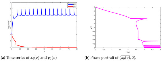
Figure 1. Globally asymptotically stable periodic solution $(\overline{x_0\left(v\right)},0)$ of system (2) setting parameters as $x_0\left(0\right)=2,$ $y_0\left(0\right)=2,$ $a_0=3,$ $K_1=5,$ ${\beta }_0=0.6,$ ${\alpha }_0=0.3,$ $k=0.461,$ $d_0=0.68,$ ${\mu }_0=1,$ $h_{max}=0.7,$ $F=5,$ $\sigma =0.3$ and ${\alpha }_1=0.3$.

Setting the model parameters as $a_0=3,K_1=5,{\beta }_0=0.5,{\alpha }_0=0.35,k=0.65$, $d_0=0.3,{\mu }_0=1,h_{max}=0.51,F=1,\sigma =0.3,$ ${\alpha }_1=0.3$ with $x_0(0)=2,$ $y_0(0)=2$ and final time $v=80,$ then $H_{11}=-d_{0}F+{\displaystyle \frac{k{\beta }_0{K}_1}{a_0({\alpha }_0{K}_1+1)}}ln{\displaystyle \frac{K_1-x_1^{*}+({\alpha }_0{K}_1+1)x_1^{*}{e}^{a_{0}F}}{K_1-x_1^{*}+({\alpha }_0{K}_1+1)x_1^{*}}}=0.3761>0,$ which implies Theorem 3 holds, so system (2) is permanent (see Figure 2).

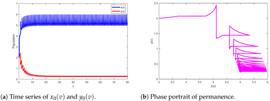
Figure 2. The permanence of the model (2) at $x_0\left(0\right)=2,$ $y_0\left(0\right)=2,$ $a_0=3,$ $K_1=5,$ ${\beta }_0=0.5,$ ${\alpha }_0=0.35,$ $k=0.65,$ $d_0=0.3,$ ${\mu }_0=1,$ $h_{max}=0.51,$ $F=1,$ $\sigma =0.3$ and ${\alpha }_1=0.3$.

In view of Theorem 3, system (2) is permanent when $H_{11}>0$ holds; however, there may be more complex dynamics. The following discussion will include several significant parameters to research more intricate behavioral dynamics of system (2). Next, we investigate the influence of the maximum harvesting ability $h_{max}$ of the predator for system (2). Set the parameters of model (2) as $a_0=1,$ $K_1=10,$ ${\beta }_0=0.8,$ ${\alpha }_0=0.15,$ $d_0=0.3,$ $k=0.41,$ ${\alpha }_1=0.15,$ ${\mu }_0=1,$ $F=3,$ $\sigma =0.53,$ $x_0(0)=0.4$ and $y_0(0)=0.2.$ Figure 3 shows the bifurcation pictures of model (2) on bifurcation parameter $h_{max}$ altering from 0.01 to 1. From Figure 3, we can see that the prey and predator will coexist periodically when $h_{max}\le 0.3667$ and $h_{max}\ge 0.7533,$ and system (2) will generate a period-doubling bifurcation when $0.3667<h_{max}<0.7533,$ that is, a route from an F-periodic solution into a $2F$-periodic stable at $h_{max}\approx 0.3667$, and a route from the $2F$-periodic solution back to an F-periodic solution for $h_{max}\approx 0.7533.$For example, a period-doubling cascade results in system from an $F-$periodic solution to a $2F-$periodic solution (see Figure 4).

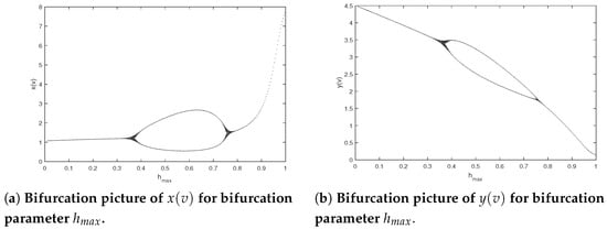
Figure 3. Bifurcation pictures of model (2) at $x_0\left(0\right)=0.4,$ $y_0\left(0\right)=0.2,$ $a_0=3,$ $K_1=10,$ ${\beta }_0=0.8,$ ${\alpha }_0=0.15,$ $k=0.41,$ $d_0=0.3,$ ${\mu }_0=1,$ ${\alpha }_1=0.15,$ $F=3$ and $\sigma =0.53,$ $0.01\le h_{max}\le 1$.

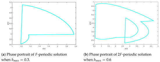
Figure 4. Period-doubling cascade results in system from an F-periodic solution to a $2F$-periodic solution setting final time $v=300$.

The next step is to research the influence of the quantity ${\mu }_0$ of impulsive stocking prey for model (2). Let the parameters of system (2) be $a_0=2,$ $K_1=25,$ ${\beta }_0=0.8,$ ${\alpha }_0=0.15,$ $d_0=0.3,$ $k=0.41,$ ${\alpha }_1=0.2,$ $h_{max}=0.45,$ $F=3,$ $\sigma =0.53,$ $x_0(0)=2$ and $y_0(0)=2.$ Figure 5 shows bifurcation pictures of $x_0(v)$ and $y_0(v)$ with bifurcation parameter ${\mu }_0$ changing from 0.01 to 12. The dynamics displayed of system (2) are complex, containing chaos, period-halving cascade, cycle, period-doubling cascade, period-halving cascade and cycles. According to Figure 5, we can obtain that system (2) will generate chaos when $0.01<{\mu }_0\le 2.88$; further increasing ${\mu }_0,$ there occurs a period-doubling bifurcation, in Figure 6, a period-halving bifurcation reduces system into a $2F-$periodic solution; moreover, periodic-halving cascade will lead the model from a $2F$-periodic solution into an F-periodic solution at ${\mu }_0\approx 5.845$; that is, the prey and predator will coexist periodically when ${\mu }_0\ge 5.845.$ And typical chaos is exhibited in Figure 7. A period-halving bifurcation results in system from a $2F-$periodic solution into an $F-$periodic solution in Figure 8.

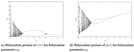
Figure 5. Bifurcation pictures of system (2) on parameters $x_0\left(0\right)=2,$ $y_0\left(0\right)=2,$ $a_0=2,$ $K_1=25,$ ${\beta }_0=0.8,$ ${\alpha }_0=0.15,$ $k=0.41,$ $d_0=0.3,$ $h_{max}=0.45,$ ${\alpha }_1=0.2,$ $F=3$ and $\sigma =0.53,$ $0.01\le {\mu }_0\le 9$.

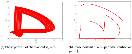
Figure 6. Period-halving bifurcation reduces system into a $2F$-periodic solution with $v=300$.

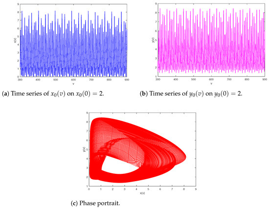
Figure 7. Chaos of prey–predator system (2) with ${\mu }_0=1$ and $v=300$.

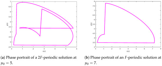
Figure 8. Period-halving bifurcation results in system from a $2F$-periodic solution into an F-periodic solution with final time $v=300$.

Lastly, we research the influence resulting from impulse period F about the dynamics of the model (2). Setting the parameters as $a_0=6,$ $K_1=25,$ ${\beta }_0=0.4,$ ${\alpha }_0=0.15,$ $d_0=0.4,$ $k=0.41,$ ${\alpha }_1=0.2,$ $h_{max}=0.6,$ ${\mu }_0=1$ and $\sigma =0.53,$ $x_0(0)=0.6$ and $y_0(0)=0.4,$ we can derive the bifurcation pictures of predator–prey model (2) with bifurcation parameter F varying from $0.01$ to 27 (see Figure 9). As shown in Figure 9, system (2) has rich behavioral dynamics, containing cycles, periodic-doubling cascade, chaos, periodic-halving cascade, periodic-doubling cascade, chaos, periodic-halving cascade, cycles, chaos, periodic-halving cascade, cycles, periodic-doubling cascade, chaos, periodic-halving cascade, periodic-doubling cascade and chaos. A typical chaos is shown in Figure 10. In Figure 11, a period-doubling cascade leads system from an $F-$periodic solution to a $2F-$periodic solution. In Figure 12, a period-halving cascade leads system from chaos to cycle. Meanwhile, the behavioral dynamics of system (2) may be altered suddenly, which is a dangerous phenomenon, such as an F-periodic solution suddenly altering into chaos when $F\approx 11.6$ if we continue to increase the impulsive period F (see Figure 13). In addition, different behavioral dynamics of system (2) will coexist for the same $F,$ which may be because of different initial values (see Figure 14). Figure 9 shows that prey and predator will periodically coexist when $F<2.98,$ further increasing F; there will be a cascade of period-doubling bifurcation leading the system from period-doubling bifurcation into chaos when $2.98\le F<5.14,$ if we maintain augmenting $F,$ a system from chaos to another period-doubling bifurcation following a cascade of periodic-halving bifurcation when $5.14\le F<6.49$, with an increase in the $F,$ and a system again from a periodic-doubling bifurcation to chaos in view of a period-doubling cascade when $6.49\le F<7.48$; if we keep adding $F,$ a period-halving cascade results in a system into cycle at $7.48\le F<9.73$; when $9.73\le F<13.33,$ the system will experience a sequence of chaos, cycle, chaos, which follows a cascade of period-halving bifurcation into cycle when $13.33\le F<20.8$; additionally, when $20.8\le F\le 27,$ system (2) will experience a sequence of periodic-doubling bifurcation, chaos, periodic-doubling bifurcation, chaos.

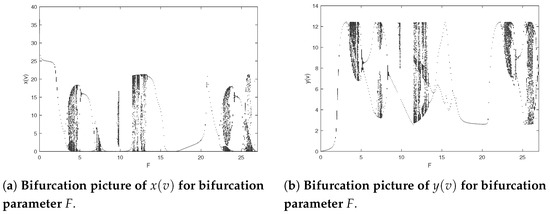
Figure 9. Bifurcation pictures of model (2) at $x_0\left(0\right)=0.6,$ $y_0\left(0\right)=0.4,$ $a_0=6,$ $K_1=25,$ ${\beta }_0=0.4,$ ${\alpha }_0=0.15,$ $k=0.41,$ $d_0=0.4,$ $h_{max}=0.6,$ ${\alpha }_1=0.2,$ $\sigma =0.53,$ ${\mu }_0=1$ and $0.01\le F\le 27$.

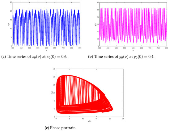
Figure 10. Chaos of prey–predator system (2) with $F=4$ and $v=2800$.

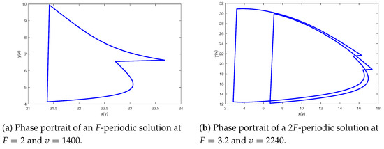
Figure 11. A period-doubling cascade leads system from an F-periodic to a $2F$-periodic solution.

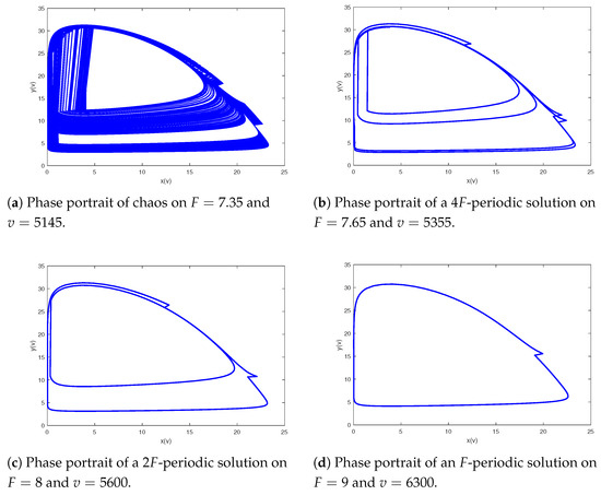
Figure 12. A period-halving cascade leads system from chaos to cycle.

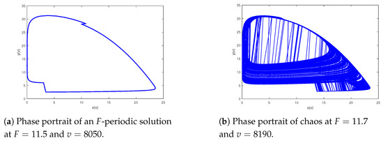
Figure 13. An F-periodic solution suddenly alters into chaos.

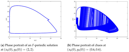
Figure 14. An F-periodic solution coexists with a strange attractor for $F=9.8$ and $v=6860$.

Reviewing Figure 3, Figure 5 and Figure 9, it is obvious that the amount of impulsive stocking prey, the maximal proportion of impulsive harvesting predators and the period of the impulse are crucial because they will determine the state of the entire system. This is because prey and predator have a mutual effect by living in the same system. That is, prey as food of the predator will significantly change the number of predators; meanwhile, the predator will hunt prey; further, the quantity of prey will be influenced by the predator. Therefore, the stocking amount of prey and the maximal harvesting rate of predator will induce dramatic transformation of the system behavioral dynamics. On the other hand, a different impulsive control period will generate a different effect for the prey–predator system; consequently, the system has different dynamics behaviors, too.

5. Conclusions

In this article, we investigated a prey–predator model, which contains impulsive stocking prey and a nonlinear harvesting predator, and the two impulses happen at different moments. We prove that the solution of model (2) is uniformly ultimately bounded. Further, we analyze that $(\overline{x_0(v)},0)$, which indicates that the predator is absent or extinct, is globally asymptotically stable; that is, the predator is extinct when the corresponding condition is satisfied by adjusting the parameters of model (2); moreover, we derive the condition on keeping system (2) permanence; based on the above results, we can conclude that the amount ${\mu }_0$ of stocking prey selected should be maintained over the threshold of the predator extinction to obtain a long-term yield. In the end, we examine our theoretical results by some numerical simulations and research the effect of the maximal harvesting ability $h_{max}$ of the predator, the quantity ${\mu }_0$ of the stocking prey and the period F of the impulse for the investigated system; then, we find that model (2) contains very complex behavioral dynamics. Further, we conclude that the selection of the quantity ${\mu }_0$ of the impulsive stocking prey, the maximal proportion $h_{max}$ of the impulsive harvesting predator and the period F of the impulse play a significant role in model (2).

Of course, there are still many questions we need to explore here. For example, what are the conditions for predator extinction and system persistence in a prey–predator system if we think about the stage structure of predators? How do we control the impulses so that we can reach an optimal harvesting? These are questions for the future to explore.

References

- Glowka, L.; Burhanne-Guilmin, F.; Synge, H.; McNeeley, J.A.; Gundling, L. A Guide to the Convention on Biological Diversity; IUCN—The World Conservation Union: Gland, Switzerland, 1994. [Google Scholar]
- Clark, C.W. Mathematical bioeconomics. In Mathematical Problems in Biology: Victoria Conference; Springer: Berlin/Heidelberg, Germany, 1974. [Google Scholar]
- Karr, J.R. Biological integrity: A long-neglected aspect of water resource management. Ecol. Appl. 1991, 1, 66–84. [Google Scholar] [CrossRef]
- Holling, C.S.; Meffe, G.K. Command and control and the pathology of natural resource management. Conserv. Biol. 1996, 10, 328–337. [Google Scholar] [CrossRef]
- Singh, J.S.; Kumar, A.; Rai, A.N.; Singh, D.P. Cyanobacteria: A precious bio-resource in agriculture, ecosystem, and environmental sustainability. Front. Microbiol. 2016, 7, 529. [Google Scholar] [CrossRef] [PubMed]
- Shannon, G.; McKenna, M.F.; Angeloni, L.M.; Crooks, K.R.; Fristrup, K.M.; Brown, E.; Warner, K.A.; Nelson, M.D.; White, C.; Briggs, J.; et al. A synthesis of two decades of research documenting the effects of noise on wildlife. Biol. Rev. 2016, 91, 982–1005. [Google Scholar] [CrossRef] [PubMed]
- Xiao, Y.; Chen, L. Modeling and analysis of a predator-prey model with disease in the prey. Math. Biosci. 2001, 171, 59–82. [Google Scholar] [CrossRef] [PubMed]
- Chattopadhyay, J.; Arino, O. A predator-prey model with disease in the prey. Nonlinear Anal. 1999, 36, 747–766. [Google Scholar] [CrossRef]
- Georgescu, P.; Hsieh, Y.H. Global dynamics of a predator-prey model with stage structure for the predator. SIAM J. Appl. Math. 2007, 67, 1379–1395. [Google Scholar] [CrossRef]
- Kazarinoff, N.D.; Van Den Driessche, P. A model predator-prey system with functional response. Math. Biosci. 1978, 39, 125–134. [Google Scholar] [CrossRef]
- Liu, X.; Chen, L. Complex dynamics of Holling type II Lotka–Volterra predator–prey system with impulsive perturbations on the predator. Chaos Solitons Fractal 2003, 16, 311–320. [Google Scholar] [CrossRef]
- Zhang, T.; Meng, X.; Song, Y.; Zhang, T. A stage-structured predator-prey SI model with disease in the prey and impulsive effects. Math. Model. Anal. 2013, 18, 505–528. [Google Scholar] [CrossRef][Green Version]
- Tsybulin, V.; Zelenchuk, P. Predator–Prey Dynamics and Ideal Free Distribution in a Heterogeneous Environment. Mathematics 2024, 12, 275. [Google Scholar] [CrossRef]
- Qin, W.; Dong, Z.; Huang, L. Impulsive Effects and Complexity Dynamics in the Anti-Predator Model with IPM Strategies. Mathematics 2024, 12, 1043. [Google Scholar] [CrossRef]
- Dai, X.; Jiao, J.; Quan, Q.; Zhou, A. Dynamics of a predator–prey system with sublethal effects of pesticides on pests and natural enemies. Int. J. Biomath. 2024, 17, 2350007. [Google Scholar] [CrossRef]
- Lv, Y.; Yuan, R.; Pei, Y. A prey-predator model with harvesting for fishery resource with reserve area. Appl. Math. Model 2013, 37, 3048–3062. [Google Scholar] [CrossRef]
- Jiao, J.; Pang, G.; Chen, L. A delayed stage-structured predator–prey model with impulsive stocking on prey and continuous harvesting on predator. Appl. Math. Comput. 2008, 195, 316–325. [Google Scholar] [CrossRef]
- Quan, Q.; Dai, X.; Jiao, J. Dynamics of a Predator–Prey Model with Impulsive Diffusion and Transient/Nontransient Impulsive Harvesting. Mathematics 2023, 11, 3254. [Google Scholar] [CrossRef]
- Jiao, J.; Cai, S.; Chen, L. Analysis of a stage-structured predator–prey system with birth pulse and impulsive harvesting at different moments. Nonlinear Anal. Real World Appl. 2011, 12, 2232–2244. [Google Scholar] [CrossRef]
- Liu, J.; Hu, J.; Yuen, P. Extinction and permanence of the predator-prey system with general functional response and impulsive control. Appl. Math. Model 2020, 88, 55–67. [Google Scholar] [CrossRef]
- Li, C.; Tang, S. Analyzing a generalized pest-natural enemy model with nonlinear impulsive control. Open Math. 2018, 16, 1390–1411. [Google Scholar] [CrossRef]
- Pang, G.; Liang, Z.; Xu, W.; Li, L.; Fu, G. A pest management model with stage structure and impulsive state feedback control. Discret. Dyn. Nat. Soc. 2015, 1, 617379. [Google Scholar] [CrossRef]
- Tan, X.; Tang, S.; Chen, X.; Xiong, L.; Liu, X. A stochastic differential equation model for pest management. Adv. Differ. Equ. 2017, 2017, 197. [Google Scholar] [CrossRef][Green Version]
- Tang, S.; Cheke, R.A. Models for integrated pest control and their biological implications. Math. Biosci. 2008, 215, 115–125. [Google Scholar] [CrossRef]
- Dai, X.; Quan, Q.; Jiao, J. Modelling and analysis of periodic impulsive releases of the Nilaparvata lugens infected with wStri-Wolbachia. J. Biol. Dynam. 2023, 17, 2287077. [Google Scholar] [CrossRef]
- Pang, G.; Chen, L.; Xu, W.; Fu, G. A stage structure pest management model with impulsive state feedback control. Commun. Nonlinear Sci. 2015, 23, 78–88. [Google Scholar] [CrossRef]
- Liu, B.; Hu, G.; Kang, B.; Huang, X. Analysis of a hybrid pest management model incorporating pest resistance and different control strategies. Math. Biosci. Eng. 2020, 17, 4364–4383. [Google Scholar] [CrossRef] [PubMed]
- Sun, K.; Zhang, T.; Tian, Y. Dynamics analysis and control optimization of a pest management predator–prey model with an integrated control strategy. Appl. Math. Comput. 2017, 292, 253–271. [Google Scholar] [CrossRef]
- Quan, Q.; Wang, M.; Jiao, J.; Dai, X. Dynamics of a predator–prey fishery model with birth pulse, impulsive releasing and harvesting on prey. J. Appl. Math. Comput. 2024, 70, 3011–3031. [Google Scholar] [CrossRef]
- Jiao, J.; Cai, S.; Li, L. Dynamics of a periodic switched predator–prey system with impulsive harvesting and hibernation of prey population. J. Franklin. Inst. 2016, 353, 3818–3834. [Google Scholar] [CrossRef]
- Liu, B.; Zhang, Y.; Chen, L. The dynamical behaviors of a Lotka–Volterra predator–prey model concerning integrated pest management. Nonlinear Anal. Real World Appl. 2005, 6, 227–243. [Google Scholar] [CrossRef]
- Guo, H.; Han, J.; Zhang, G. Hopf bifurcation and control for the bioeconomic predator-prey model with square root functional response and nonlinear prey harvesting. Mathematics 2023, 11, 4958. [Google Scholar] [CrossRef]
- Lakshmikantham, V. Theory of Impulsive Differential Equations; World Scientific: Singapore, 1989. [Google Scholar]
Disclaimer/Publisher’s Note: The statements, opinions and data contained in all publications are solely those of the individual author(s) and contributor(s) and not of MDPI and/or the editor(s). MDPI and/or the editor(s) disclaim responsibility for any injury to people or property resulting from any ideas, methods, instructions or products referred to in the content. |
© 2024 by the authors. Licensee MDPI, Basel, Switzerland. This article is an open access article distributed under the terms and conditions of the Creative Commons Attribution (CC BY) license (https://creativecommons.org/licenses/by/4.0/).