MMCMOO: A Novel Multispectral Pansharpening Method

Abstract

From the perspective of optimization, most of the current mainstream remote sensing data fusion methods are based on traditional mathematical optimization or single objective optimization. The former requires manual parameter tuning and easily falls into local optimum. Although the latter can overcome the shortcomings of traditional methods, the single optimization objective makes it unable to combine the advantages of multiple models, which may lead to distortion of the fused image. To address the problems of missing multi-model combination and parameters needing to be set manually in the existing methods, a pansharpening method based on multi-model collaboration and multi-objective optimization is proposed, called MMCMOO. In the proposed new method, the multi-spectral image fusion problem is transformed into a multi-objective optimization problem. Different evolutionary strategies are used to design a variety of population generation mechanisms, and a non-dominated sorting genetic algorithm (NSGA-II) is used to optimize the two proposed target models, so as to obtain the best pansharpening quality. The experimental results show that the proposed method is superior to the traditional methods and single objective methods in terms of visual comparison and quantitative analysis on our datasets.

1. Introduction

In the process of satellite remote sensing imaging, limited by the sensing ability of sensors, it is difficult to directly obtain images with both high spatial resolution and high spectral resolution. Typically, panchromatic images have very high spatial resolution but lack spectral information, while hyperspectral images have high spectral resolution but relatively low spatial resolution. Pansharpening technology is an effective way to compensate for the lack of imaging hardware. Using pansharpening, we can fuse the spatial information of panchromatic images with the spectral information of hyperspectral images, so as to obtain high-quality remote sensing images with more comprehensive information.

Generally speaking, pansharpening methods can be divided into two categories: spatial domain methods and transformation domain methods. Spatial domain methods mainly include the high-pass filtering fusion method [1], Brovey [2], BDSD [3], etc. The main methods in the transformation domain include Intensity-Hue-Saturation (IHS) [4], Principal Component Analysis (PCA) [5,6], Laplacian pyramid method [7], Wavelet [8], etc. If classified according to the research results, pansharpening methods can be divided into four categories: ① Methods based on color space, such as IHS [4], Adapt IHS (AIHS) [9], and so on; ② Methods based on mathematical statistics, such as ratio operation [10], FANG [11], SIRF [12], VWP/AVWP [13,14], etc.; ③ Methods based on the multi-resolution analysis method (MRA) [15,16], such as the pyramid method [7], Wavelet [8], etc. ④ Methods based on intelligent computing, such as evolutionary computing [17], neural networks [18,19,20], and deep learning [21,22,23,24].

Most of the above methods are based on traditional mathematical optimization or single objective optimization, so they have the following two shortcomings:

(1)

In traditional mathematical optimization methods, model parameters need to be adjusted manually, which is time-consuming and laborious, and it is easy to fall into local optimal solutions, which will lead to contrast distortion and aliasing of the fused image [25].

(2)

Although the single-objective intelligent optimization algorithm avoids manual parameter adjustment, due to the limitations of a single optimization objective, this kind of method cannot consider multiple factors and optimize multiple objectives at the same time, which will lead to imbalance between spectral information and spatial information, resulting in blurring, ghosting, flare and other phenomena in pansharpened images [26].

In recent years, multi-objective evolutionary algorithms have been initially applied in the field of remote sensing image processing and have shown unique advantages. In [27], Li et al. proposed a method based on the combination of non-downsampled contourlet transform (NSCT) and multi-objective optimization. In this method, two quality evaluation indexes are used as objective functions by using the regional consistency fusion rules, and then the multi-objective evolutionary algorithm (MOEA) is adopted to optimize them. Although this method achieves relatively good fusion quality, there is still slight distortion [28].

In [29], based on the theory of DT-CWT, Xie et al. took the absolute value of high-frequency transform coefficient as the fusion rule, the fusion weight in low-frequency sub-band as particles, the spatial frequency and average gradient as two objective functions, and then used MOPSO to optimize these two objectives. Experimental results show that this method is superior to the average fusion method and the fusion method based on local variance and local energy in brightness and clarity, but the fusion quality of this method still has much room for improvement [30].

In [31], Zhang et al. combined two conflicting clustering validity indexes with a multi-objective search algorithm (DMMOGSA), and proposed an RSI classification method based on multi-objective optimization. Because this method is not for image fusion, it uses a multi-objective optimization method in remote sensing technology, which brings us inspiration to a certain extent. Wu et al. [32] proposed a novel multi-objective guided divide-and-conquer network (MO-DCN). It consists of a deconvolution long-term and short-term memories (LSTMs) network (DLSTM) and a divide-and-conquer network (DCN). In this method, the common improvement of spatial and spectral information is expressed as an Epsilon-constraint-based multi-objective optimization. In addition, the Epsilon constraint method transforms a goal into a constraint and regards it as a penalty bound to make a good trade-off between different goals. Although this method has achieved good fusion effect, its time complexity is high [33].

Most of the above methods choose a variety of different fusion rules, multiple different evaluation indicators, or multiple different weight parameters, but rarely choose multiple fusion models. This is mainly because it is very complicated to establish several suitable fusion models and optimize them at the same time. In addition, the values of multiple parameters of multiple models are often mutually exclusive. If the values of these parameters continue to be set manually, there will be local optimization problems. As a result, the fused image will exhibit spectral distortion. To this end, this paper proposes a multispectral pansharpening method, called MMCMOO, which combines the more advanced multi-objective optimization strategies NSGA-II [34,35] and AIHS transformation [9], to overcome the problems of multi-model missing and manual parameter setting, and further improves the fusion accuracy. In this method, the pansharpening problem of multispectral images and panchromatic images is transformed into a multi-objective optimization problem. Three different evolutionary strategies are adopted to design a variety of population generation mechanisms. The crossover operator and mutation operator in the NSGA-II algorithm are improved, and then the two models are optimized in parallel by using the improved NSGA-II algorithm. In addition, a one-step local search operator is proposed to improve the convergence speed of the algorithm.

2. Multi-Objective Fusion Model

The technical route of MMCMOO is shown in Figure 1, and the details of this method will be introduced next.

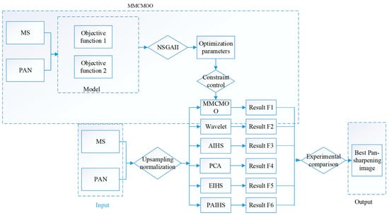
Figure 1. The technical route of MMCMOO.

2.1. Multi-Objective Fusion Problem and Definition

In order to realize the fusion of multispectral and panchromatic images, the modeling of the pansharpening problem usually requires meeting the two premise assumptions of spatial information consistency and spectral information consistency [17], which are briefly introduced as follows.

(1) The strategy of keeping spatial information. Assuming that the spatial resolution data of the panchromatic image P is equal to the linear combination of the spatial data of each band component in the pansharpened image F (with N bands), its mathematical expression is as follows

$$\mathrm{P}\approx {{\displaystyle \sum }}_n{\theta }_n{F}_n,$$

(1)

where${\theta }_n$ is an unknown coefficient, and 0 $\le {\theta }_n\le 1$, $n=\left(1,2,\dots ,N\right)$. $F_n$ denotes the $nth$ band image of F.

(2) The strategy of maintaining spectral information. Assuming that the MS M is a synthesis of up-sampled or down-sampled images obtained by spatial convolution of all components of pansharpening F, its expression is as follows

$$M_n\left(x,y\right)\approx {{\displaystyle \sum }}_{i,j}K\left(i,j\right)F_n\left(x-i,y-j\right),$$

(2)

where $K\left(i,j\right)$ is a 3 × 3 convolution model, $i,j=1, 2, 3$. $M_n$ denotes the $nth$ band image of M.

These two hypotheses are based on the basic principle of remote sensing image pan sharpening. The purpose is to establish association constraints between pansharpened image F and panchromatic image PAN, as well as pansharpened image F and multispectral image MS. Its rationality has been verified by experiments in the literature [17]. In order to keep the spectral resolution of MS and the spatial resolution of PAN at the same time, the following objective function H can be designed according to the above two assumptions:

$$\begin{gathered} minH\left(\alpha ,\theta ,K\right)={{\displaystyle \sum }}_{x,y}\{{|P\left(x,y\right)-{{\displaystyle \sum }}_n{\theta }_n{F}_n\left(x,y\right)|}^p+ \\ {\displaystyle \frac{1}{N}}{{\displaystyle \sum }}_n{|M_n\left(x,y\right)-{{\displaystyle \sum }}_{i,j}K\left(i,j\right)F_n\left(x-i,y-j\right)|}^p\}, \\ s.t. 0\le {\alpha }_n\le 1,n=1, 2, \dots , N \\ {\theta }_n\le 1,n=1, 2, \dots , N \\ {{\displaystyle \sum }}_{i,j}K\left(i,j\right)=1, 0\le K\left(i,j\right)\le 1, i,j=1,2,3. \end{gathered}$$

(3)

where${\alpha }_n$ and ${\theta }_n$ are nonnegative unknown coefficients, N represents the number of bands. In this paper, H is taken as the first objective function $Z_1$, and then

$$\begin{gathered} Z_1={{\displaystyle \sum }}_{x,y}\{{|P\left(x,y\right)-{{\displaystyle \sum }}_n{\theta }_n{F}_n\left(x,y\right)|}^p+{\displaystyle \frac{1}{N}}{{\displaystyle \sum }}_n{|M_n\left(x,y\right)-{{\displaystyle \sum }}_{i,j}K\left(i,j\right)F_n\left(x-i,y-j\right)|}^p\} \\ s.t. 0\le {\alpha }_n\le 1, n=1, 2, \dots , N \\ 0\le {\theta }_n\le 1, n=1, 2, \dots , N \\ {{\displaystyle \sum }}_{i,j}K\left(i,j\right)=1, 0\le K\left(i,j\right)\le 1, i,j=1,2,3. \end{gathered}$$

(4)

In fact, even when Formula (3) obtains the optimal value, it does not necessarily mean that the optimal fusion quality can be obtained. Therefore, it is necessary for us to further constrain the components of Equation (3), so the second objective $Z_2$is defined as

$$Z_2={{\displaystyle \sum }}_{x,y}\{{\left|P\left(x,y\right)-{{\displaystyle \sum }}_n{\theta }_n{F}_n\left(x,y\right)\right|}^p.$$

(5)

In these two models, $Z_1$ is optimised for a minimum value with the aim of ensuring that the best spatial and spectral quality is retained in pansharpened images. $Z_2$ is to ensure that the spatial information division can get the minimum value, that is, to ensure that the best spatial resolution is retained in the pansharpened image.

2.2. NSGA-II Optimization

Because of the high time complexity and unreasonable sharing radius of the non-dominated sorting genetic algorithm (NSGA), an NSGA-II algorithm is proposed by introducing the elite reservation strategy [36].

2.2.1. Coding Mode

According to the previous section, the objective functions to be optimized are $Z_1$ and $Z_2$. Parameters to be optimized in $Z_1$ include α, θ and K, where α is a group of vectors (${\alpha }_1, \dots ,{\alpha }_N)$ of length N, θ is a group of vectors $({\theta }_1, \dots , {\theta }_N)$ of length N, and K is a $3\times 3$ filter $(K_{11},K_{12},K_{13},K_{21},K_{22},K_{23},K_{31},K_{32},K_{33}).$ For the objective function $Z_1$, there are $2\ast N+9$ parameters to be optimized. Parameters to be optimized in $Z_2$ include α and θ, where α is a group of vectors $({\alpha }_1, \dots , {\alpha }_N)$ of length N, and θ is a group of vectors $({\theta }_1, \dots ,{\theta }_N)$ of length N. For the objective function $Z_2$, there are 2*N parameters to be optimized. These parameters to be optimized are expressed by chromosome coding in the NSGA-II algorithm, which is shown in Figure 2.

Figure 2. The chromosome representation.

In this paper, r is used to represent a chromosome, and, $r_i\left(i=1, \dots , 2N+9\right)\in \left[0,1\right]$ represents the genes in this chromosome. $\left\{r_1, \dots ,{\mathrm{r}}_N\right\}$ corresponds to $\left({\alpha }_1, \dots ,{\mathsf{\alpha }}_N\right)$, $\left\{r_{N+1}, \dots ,{ \mathrm{r}}_{2N}\right\}$ corresponds to $\left({\theta }_1, \dots ,{\theta }_N\right)$, and $\left\{r_{2N+1}, \dots , r_{2N+9}\right\}$ corresponds to $\left({\mathrm{K}}_{12},{\mathrm{K}}_{13},{\mathrm{K}}_{21},{\mathrm{K}}_{22},{\mathrm{K}}_{23},{\mathrm{K}}_{31},{\mathrm{K}}_{32},{\mathrm{K}}_{33}\right)$. Because the three parameters α, θ and K need to be normalized, the first step of decoding is to map chromosomes into feasible solutions of the three parameters. The decoding method is as follows

$${\alpha }_n={\displaystyle \frac{r_n}{{{\displaystyle \sum }}_{i=1}^N{r}_i}},$$

(6)

$${\theta }_n={\displaystyle \frac{r_{N+n}}{{{\displaystyle \sum }}_{i=N+1}^{2N}{r}_i}},$$

(7)

$$K_{ml}={\displaystyle \frac{r_{3\left(m-1\right)+l+2N}}{{{\displaystyle \sum }}_{i=2N+1}^{2N+9}{r}_i}}.$$

(8)

2.2.2. The Population Initialization

The population size is set to $Po{p}_{-}Size$, and the maximum algebra is set to $ma{x}_{-}t$. Use $Pop\left(t\right)={\left[r^h\left(t\right)\right]}_{Po{p}_{-}Size}$ to represent the population of generation $t$, where $r^h\left(t\right)$ represents the $h$ chromosome of generation $t$. $r^h\left(t\right)$ can be described as $r^h\left(t\right)=\left\{r_1^h\left(t\right), \dots ,r_{2N+9}^h\left(t\right)\right\}$, $r_i^h\left(t\right)$ represents the ith gene on the chromosome, and $h\in \left\{1,\dots ,Pop\_size\right\}$ represents an integer.

In order to shorten the calculation time and make the candidate solution approach the optimal solution with a higher probability, three strategies are used to generate the initial population $Pop\left(0\right)={\left[r^h\left(0\right)\right]}_{po{p}_{size}}$.

Strategy 1 (CoDE+Z1): Use the combined differential evolution algorithm (CoDE) to optimize the $Z_1$ model. Because the purpose of this strategy is to generate the initial population, only the running algebra of CoDE algorithm is set to 10, and the population size is set to $Po{p}_{-}Size$. At the 10th generation, the best first $\lfloor {\beta }_2\times Pop\_size\rfloor$ chromosomes are selected as the initial population of the NSGA-II algorithm, where ${\beta }_2\in \left(0,1\right)$ represents the coefficient of the population generated by strategy 1.

Strategy 2 (CoDE+Z2): Use CoDE algorithm to optimize Z2 model. Similarly, set the running algebra of the CoDE algorithm to 10 and the population size to $Po{p}_{-}Size$. At the 10th generation, the best first $\lfloor {\beta }_4\times Pop\_size\rfloor$ chromosomes are selected as the initial population of the NSGA-II algorithm, where ${\beta }_4\in \left(0,1\right)$ represents the coefficient of the population generated by strategy 2.

Strategy 3 (Random): Randomly generate$Po{p}_{-}Size-\lfloor {\beta }_2\times Po{p}_{size}\rfloor -\lfloor {\beta }_4\times Pop\_size\rfloor$ initial populations.

Three strategies are used to generate the initial population, and the parameters ${\beta }_2$ and ${\beta }_4$ are used to adjust the proportion of each strategy to generate the initial population. In order to make the initial population have better diversity, the randomly generated population in strategy 3 can be given a larger weight. The purpose of strategy 1 and strategy 3 is to improve the convergence of obtaining the optimal solution. Strategies 1 and 2 can not only ensure the diversity of the initial solution, but also ensure the convergence of the optimal solution. The initial population generation strategy is shown in Figure 3.

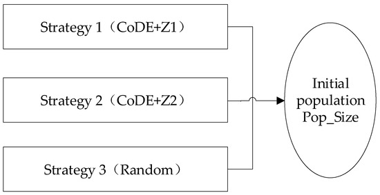
Figure 3. Population generation strategy.

2.2.3. Evolutionary Operator Design

Evolutionary operators in the NSGA-II algorithm mainly include the simulated binary crossover operator, polynomial mutation operator, and fast non-dominated sorting selection operator. In addition, crowding distance and elite retention mechanism are also added. Among them, the main function of the evolution operator is to generate the next generation feasible solution. In this paper, for the $t$generation population $Pop\left(t\right)={\left[r^h\left(t\right)\right]}_{Po{p}_{-}Size}$, the $t+1$ generation population $Pop\left(t\right)={\left[r^h\left(t+1\right)\right]}_{Po{p}_{-}Size}$ is generated by using an improved evolutionary operator. Next, these evolutionary operators will be briefly introduced.

(1)

Binary crossover operator

The binary crossover operator is a common operator in the NSGA-II algorithm. For the $t$ generation population $Pop\left(t\right)={\left[r^h\left(t+1\right)\right]}_{Po{p}_{-}Size}$, an intermediate population $PC\left(t\right)={\left[r{c}^h\left(t\right)\right]}_{Po{p}_{-}Size}$ can be obtained by using the simulated binary crossover operator, where $r{c}^h$ represents the H chromosome. For two chromosomes $r^A\left(t\right)={\left[r_i^A\left(t\right)\right]}_{2N+9}$ and $r^B\left(t\right)={\left[r_i^B\left(t\right)\right]}_{2N+9}$ in generation t, the simulated binary crossover operator can be used to generate two intermediate chromosomes [$r{c}^A\left(t\right)={\left[r{c}_i^A\left(t\right)\right]}_{2N+9}$and $r{c}^B\left(t\right)={\left[r{c}_i^B\left(t\right)\right]}_{2N+9}, i\in \left\{1,\dots ,2N+9\right\}$, where $r_i^A\left(t\right)$ and $r_i^B\left(t\right)$ represents the ith gene on chromosomes A and B. The formula can be described as

$$r{c}_i^A\left(t\right)=0.5\ast \left[\left(1+{\gamma }_i\right)r_i^A\left(t\right)+\left(1-{\gamma }_i\right)r_i^B\left(t\right)\right],$$

(9)

$$r{c}_i^B\left(t\right)=0.5\ast \left[\left(1-{\gamma }_i\right)r_i^A\left(t\right)+\left(1+{\gamma }_i\right)r_i^B\left(t\right)\right],$$

(10)

where ${\gamma }_i$ satisfies

$${\gamma }_i=\left\{\begin{array}{c}{(2u_i)}^{{\displaystyle \frac{1}{\tau +1}}}{u}_i<0.5\\ {\displaystyle \frac{1}{{(2\left(1-u_i\right))}^{\frac{1}{\tau +1}}}}else\end{array}\right.$$

(11)

where $u_i\in U\left(0,1\right)$, $\tau >0$ represents the distribution index.

(2)

Polynomial mutation operator

The operator is designed based on the binary crossover operator mentioned above, which is a common operator in real number mutation, and it can generate a new group of mutation populations according to the probability. For the population $PC\left(t\right)={\left[r{c}^h\left(t\right)\right]}_{Po{p}_{-}Size}$ obtained after the crossover operation, a new group of mutant populations $PM\left(t\right)={\left[r{m}^h\left(t\right)\right]}_{Po{p}_{-}Size}$ can be generated by using the polynomial mutation operator.

For a crossed chromosome $r{c}^A\left(t\right)={\left[r{c}_i^A\left(t\right)\right]}_{2N+9}$, its polynomial variation can be described as

$$r{m}_i^A\left(t\right)=r{c}_i^A\left(t\right)+{\Delta }_i,$$

(12)

where ${\Delta }_i=\left\{\begin{array}{c}{(2u_i)}^{{\displaystyle \frac{1}{\tau +1}}}-1 u_i<0.5\\ 1-{\displaystyle \frac{1}{{(2\left(1-u_i\right))}^{\frac{1}{\tau +1}}}} else\end{array}\right.$.

(3)

Combinatorial differential evolution operator

In order to increase the diversity of each generation population and make the population fall into the optimal solution quickly, an improved combined differential evolution operator is used to generate new populations. By using this operator, the T-generation population $P\left(t\right)={\left[r^h\left(t\right)\right]}_{Po{p}_{-}Size}$ can generate the differential population $PD\left(t\right)={\left[r{d}^h\left(t\right)\right]}_{Po{p}_{-}Size}$. Here, two factors need to be considered: population diversity and rapid convergence. For more details, please refer to [37].

First, population diversity needs to be considered. For chromosome A: $r{d}^A\left(t\right)={\left[r{d}_i^A\left(t\right)\right]}_{2N+9}$, the generation rule is

$$r{d}_i^A\left(t\right)=\left\{\begin{array}{c}{r}_i^{r1}\left(t\right)+{\lambda }_1\left(r_i^{r2}\left(t\right)-r_i^{r3}\left(t\right)\right)IF ran{d}_i<C{r}_1 or i=i_{rand}\\ r_i^A\left(t\right)otherwise\hfill \end{array}\right.,$$

(13)

where $r_1$, $r_2$ and $r_3$ are three different integers, which should be randomly selected from $\left\{1,\dots ,Po{p}_{-}Size\right\}$. ${\lambda }_1$ is a regulating factor, which mainly controls the weight of the two parts. $ran{d}_i$ is a real number randomly generated in the range of [0,1], and its value is different for each gene. $C{r}_1=\left[0,1\right]$ indicates the crossover factor, which needs to be set in advance. $i_{rand}$ represents an integer randomly selected in $\left\{1,\dots ,2N+9\right\}$.

Secondly, the population convergence needs to be considered in the algorithm improvement. For chromosome A: $r{d}^A\left(t\right)={\left[r{d}_i^A\left(t\right)\right]}_{2N+9}$, the generation rule is

$$r{d}_i^A\left(t\right)=\left\{\begin{array}{c}{r}_i^{bes{t}_A}\left(t\right)+{\lambda }_2\left(r_i^{r1}\left(t\right)-r_i^A\left(t\right)\right)IF ran{d}_i<C{r}_2 or i=i_{rand}\\ r_i^A\left(t\right)otherwise\hfill \end{array}\right.$$

(14)

In the above formula,${\lambda }_2$ and ${\lambda }_1$ have the same function, and $r^{bes{t}_A}\left(t\right)$ represents the best solution set relative to $r^A\left(t\right)$.

Usually, the best solution in each generation of a population is located at the front of the Pareto set. However, since the Pareto front contains multiple solution sets, how to select the best solution set is also a problem to be solved. In this paper, a method which can quickly find the optimal solution set of the current population is designed. The idea is as follows.

For chromosome $r^A\left(t\right)$, the optimal solution set should be on the line from the target function of the chromosome to the target function of the reference point. Therefore, first draw the connection, and then select the solution closest to the connection in the Pareto solution set. The chromosome corresponding to these solutions is the optimal solution set of the individual. The method is shown in Figure 4.

Figure 4. Pareto optimal solution selection strategy.

In Figure 4, Z* is the reference point, and PF1, PF2, PF3 and PF4 are four Pareto solution sets. Next, select the optimal solution set as $r^{bes{t}_A}\left(t\right)$ in these four Pareto solution sets. In Figure 4, draw four vertical lines from the Pareto points to$r^A\left(t\right)Z^{*}$. It is obvious that PF2 is the closest to the line, so PF2 can be considered as the optimal solution set $r^{bes{t}_A}\left(t\right)$. The specific steps are shown in Algorithm 1.

In the above, we used two operators to obtain the differential population $PD\left(t\right)={\left[r{d}^h\left(t\right)\right]}_{Po{p}_{-}Size}$. Because the first operator aims to expand the diversity of the population, the second operator aims to improve the convergence of the population. Therefore, we need to use a parameter $mut{a}_{-}\alpha$ to adjust the ratio of the two operators. The number of populations generated by the first operator is $\lfloor mut{a}_{-}\alpha \ast Po{p}_{-}Size\rfloor$, and the number of populations generated by the second operator is $Po{p}_{-}Size-\lfloor mut{a}_{-}\alpha \ast Po{p}_{-}Size\rfloor$. In the early stage of the algorithm implementation, we hope that the diversity of the population will be wider, while in the later stage, we hope that the population will tend to converge. Based on this, the calculation method of $mut{a}_{-}\alpha$ can be described as follows

$$muta\_\alpha =\mathit{exp}(1-{\displaystyle \frac{\mathit{max}\_t}{\left(\mathit{max}\_t+1-t\right)}})$$

(15)

In order to make the value of each chromosome fall within the range of $\left[0,1\right]$, we should revise the chromosome after the genetic operation. $Pop\left(i,j\right)$ represents the $j$ element in the $i$ chromosome of population Pop, and its repair mode during operation is expressed by the following formula:

$$Pop\left(i,j\right)=\left\{\begin{array}{c}rand\left(0.5, 1.0\right) if Pop\left(i,j\right)>1\\ rand\left(0.0, 0.5\right) if Pop\left(i,j\right)<0 \\ Pop\left(i,j\right) otherwise \end{array}\right.$$

(16)

where rand( ) is expressed as a random value between [0,1].

Algorithm 1: Solving the Optimal Pareto Solution

Input: $\mathrm{Initial} \mathrm{chromosome} r^A\left(t\right)$, Pareto solution set Output: $\mathrm{Optimal} \mathrm{solution} \mathrm{set} r^{bes{t}_A}\left(t\right)$ Step 1: $\mathrm{Calculate} \mathrm{the} \mathrm{reference} \mathrm{point}. \mathrm{The} \mathrm{reference} \mathrm{point} Z^{*}=\left(\min Z_1,\min Z_2\right)$ is calculated and obtained by minimizing Z1 and Z2. Step 2: $\mathrm{Calculate} {\mathrm{Z}}_1 \mathrm{and} {\mathrm{Z}}_2 \mathrm{function} \mathrm{values} \mathrm{of} r^A\left(t\right)$$\mathrm{respectively}, \mathrm{and} \mathrm{calculate} \mathrm{its} \mathrm{coordinates} \left(Z_1\left(r^A\left(t\right),Z_2\left(r^A\left(t\right)\right)\right)\right)$. Step 3: $\mathrm{Calculate} \mathrm{the} \mathrm{connecting} \mathrm{line} \mathrm{between} \mathrm{the} \mathrm{coordinates} \left(Z_1\left(r^A\left(t\right),Z_2\left(r^A\left(t\right)\right)\right)\right)$$\mathrm{in} \mathrm{solution} \mathrm{space} r^A\left(t\right)$$\mathrm{and} \mathrm{the} \mathrm{reference} \mathrm{point} Z^{*}=\left(\min Z_1,\min Z_2\right)$. Step 4: Calculate the perpendicular lines from all Pareto front solutions to connecting lines respectively, and record their distances. Step 5: $\mathrm{Find} \mathrm{the} \mathrm{minimum} \mathrm{vertical} \mathrm{distance} \mathrm{and} \mathrm{take} \mathrm{the} \mathrm{Pareto} \mathrm{solution} \mathrm{as} r^{bes{t}_A}\left(t\right)$.

(4)

Local search operator

In order to improve the convergence of the algorithm, a new local search operator is added to the algorithm. For each chromosome $r^h\left(t\right)$, the CoDE algorithm can also be used to perform two single-step local searches on the Z1 and Z2 functions, so as to obtain new chromosomes $Z_1{r}^h\left(t\right)={\left[Z_1{r}_i^h\left(t\right)\right]}_{2N+9}$ and $Z_2{r}^h\left(t\right)={\left[Z_2{r}_i^h\left(t\right)\right]}_{2N+9}$ after two local searches. The calculation method of this operation is shown in Figure 5.

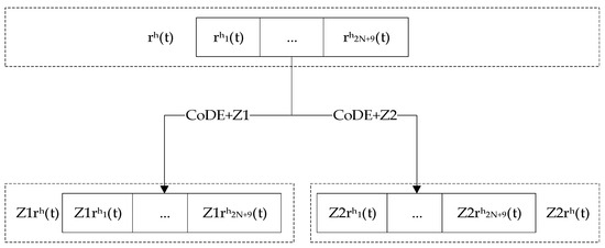
Figure 5. One-step local search operator.

By performing this operation on each t-generation chromosome, two single-step search populations, $Z_{1}Pop\left(t\right)={\left[Z_1{r}^h\left(t\right)\right]}_{Po{p}_{-}Size}$ and $Z_{2}Pop\left(t\right)={\left[Z_2{r}^h\left(t\right)\right]}_{Po{p}_{-}Size}$, can be obtained.

(5)

Non-dominated sorting and selection operators

After the above four evolutionary operator operations, five groups of populations can be obtained, which are the t-generation population $Pop\left(t\right)={\left[r^h\left(t\right)\right]}_{Po{p}_{-}Size}$, mutant population $PM\left(t\right)={\left[r{m}^h\left(t\right)\right]}_{Po{p}_{-}Size}$, differential population $PD\left(t\right)={\left[r{d}^h\left(t\right)\right]}_{Po{p}_{-}Size}$, and two one-step searches for populations $Z_{1}Pop\left(t\right)={\left[Z_1{r}^h\left(t\right)\right]}_{Po{p}_{-}Size}$ and $Z_{2}Pop\left(t\right)={\left[Z_2{r}^h\left(t\right)\right]}_{Po{p}_{-}Size}$. Next, $Po{p}_{-}Size$ high-quality solutions are selected from the five groups of populations as the next generation population $Pop\left(t+1\right)={\left[r^h\left(t+1\right)\right]}_{Po{p}_{-}Size}$.

1)

Fast non-dominated sorting algorithm

The algorithm needs to calculate two parameters $n_p$ and $S_p$ of each individual $r^h\left(t\right)$ in the population $Po{p}_{-}Size$, where $n_p$ is the number of dominant individuals $r^h\left(t\right)$ in all individuals in the population and $S_p$ is the set of individuals dominated by individuals $r^h\left(t\right)$ in the population. The main steps of this algorithm are shown in Algorithm 2.

Algorithm 2: Fast Nondominated Sorting Algorithm

Step 1: Find the individuals with non-dominant solutions in the population, that is, all individuals with$r^h\left(\mathrm{t}\right)=0$$, \mathrm{and} \mathrm{save} \mathrm{them} \mathrm{in} \mathrm{the} \mathrm{current} \mathrm{set} F_1$(s);

Step 2:$\mathrm{Set} F_1\left(s\right)$ is defined as the first-level non-dominated set, and each individual in $F_1\left(s\right)$ is marked with the same non-dominated sequence $P_{rank}$. At the same time, for each individual i in $F_1\left(s\right)$$, \mathrm{the} \mathrm{dominant} \mathrm{individual} \mathrm{is} S_{\mathrm{i}}$$, \mathrm{each} \mathrm{individual} r^h\left(s\right)$$\mathrm{in} S_{\mathrm{i}}$$\mathrm{is} \mathrm{traversed}, \mathrm{and} \mathrm{the} \mathrm{minus} 1 \mathrm{operation} \mathrm{is} \mathrm{performed} \mathrm{on} {\mathrm{n}}_l$$, \mathrm{which} \mathrm{is} \mathrm{expressed} \mathrm{as} {\mathrm{n}}_l={\mathrm{n}}_l-1$$. \mathrm{If} {\mathrm{n}}_l=0$$, \mathrm{then} \mathrm{the} \mathrm{individual} r^h\left(s\right)$$\mathrm{is} \mathrm{stored} \mathrm{in} \mathrm{the} \mathrm{set} F_{nl}\left(H\right)$;

Step 3: The individuals obtained in $F_1\left(s\right)$ are taken as the individuals of the first non-dominant layer, and $F_{nl}\left(H\right)$ is taken as the current set;

Step 4:$\mathrm{Repeat} \mathrm{steps} 1, 2 \mathrm{and} 3 \mathrm{for} \mathrm{all} \mathrm{individuals} \mathrm{in} \mathrm{the} \mathrm{set} F_{nl}\left(H\right)$ until all individuals in the population are layered.

2)

Calculation of crowding degree and crowding distance

Crowding refers to the density of individuals in a population, as shown in Figure 6.

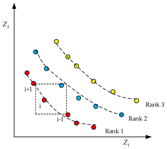
Figure 6. Pareto Frontier and Crowding Distance.

The formula for calculating the congestion distance is as follows

$$D_i=\left(Z_{i+1,1}-Z_{i-1,1}\right)+\left(Z_{i-1,2}-Z_{i+1,2}\right),$$

(17)

where $D_i$ represents the sum of the length and width of the dotted quadrilateral in Figure 6. The algorithm steps of crowding degree are shown in Algorithm 3.

Algorithm 3: Crowding degree and crowding distance

Step 1: $\mathrm{Set} {\mathrm{n}}_d=0$$, \mathrm{m}\in 1\dots \mathrm{Pop}\_\mathrm{Size}$;

Step 2: $\mathrm{For} \mathrm{each} \mathrm{objective} \mathrm{function} Z_{\mathrm{m}}$: ①$\mathrm{According} \mathrm{to} \mathrm{the} \mathrm{objective} \mathrm{function}, \mathrm{rank} \mathrm{the} \mathrm{individuals} \mathrm{of} \mathrm{this} \mathrm{grade}, \mathrm{and} {\mathrm{Z}}_m^{m\mathrm{in}}<Z_m<{\mathrm{Z}}_m^{max}$; ②$\mathrm{The} \mathrm{crowding} \mathrm{degree} \mathrm{of} \mathrm{the} \mathrm{sorted} \mathrm{two} \mathrm{edges} {\mathrm{l}}_d$$\mathrm{and} N_{\mathrm{d}} \mathrm{is} \mathrm{set} \mathrm{to} \infty$; ③ $\mathrm{Calculate} {\mathrm{n}}_d={\mathrm{n}}_d+\left(Z_m\left(\mathrm{i}+1\right)-Z_m\left(\mathrm{i}-1\right)\right)/\left({\mathrm{Z}}_m^{max}-{\mathrm{Z}}_m^{m\mathrm{in}}\right)$$, \mathrm{where} Z_m\left(\mathrm{i}+1\right)$ is the last objective function value of the individual ranking.

3)

Elite retention strategy

The purpose of elite retention is to retain the better individuals in $Pop\left(t\right)={\left[r^h\left(t\right)\right]}_{Po{p}_{-}Size}$ to directly enter the offspring population $PD\left(t\right)={\left[r{d}^h\left(t\right)\right]}_{Po{p}_{-}Size}$. The operation steps are shown in Algorithm 4:

Algorithm 4: Elite Retention Strategy Algorithm

Step 1: $\mathrm{Parent} \mathrm{population} Pop\left(t\right)={\left[r^h\left(t\right)\right]}_{Po{p}_{-}Size}$$\mathrm{and} \mathrm{offspring} \mathrm{population} PD\left(t\right)={\left[r{d}^h\left(t\right)\right]}_{Po{p}_{-}Size}$$\mathrm{Synthetic} \mathrm{population} R_{\mathrm{i}}\left(\mathrm{t}+1\right)$;

Step 2$: \mathrm{Generate} \mathrm{a} \mathrm{new} \mathrm{parent} \mathrm{population} R_{\mathrm{i}}\left(\mathrm{t}+2\right)$$\mathrm{from} \mathrm{population} R_{\mathrm{i}}\left(\mathrm{t}+1\right)$ according to the following rules: ① $\mathrm{According} \mathrm{to} \mathrm{the} \mathrm{order} \mathrm{of} \mathrm{Pareto} \mathrm{grade} \mathrm{from} \mathrm{low} \mathrm{to} \mathrm{high}, \mathrm{the} \mathrm{whole} \mathrm{layer} \mathrm{population} \mathrm{is} \mathrm{put} \mathrm{into} \mathrm{the} \mathrm{parent} \mathrm{population} R_{\mathrm{i}+1}$$\mathrm{until} \mathrm{all} \mathrm{the} \mathrm{individuals} \mathrm{in} \mathrm{a} \mathrm{certain} \mathrm{layer} \mathrm{can} \mathrm{not} \mathrm{be} \mathrm{put} \mathrm{into} \mathrm{the} \mathrm{parent} \mathrm{population} R_{\mathrm{i}+1}\left(\mathrm{t}+1\right)$; ② $\mathrm{The} \mathrm{individuals} \mathrm{in} \mathrm{this} \mathrm{layer} \mathrm{are} \mathrm{placed} \mathrm{in} \mathrm{the} \mathrm{parent} \mathrm{population} R_{\mathrm{i}+1}\left(\mathrm{t}+1\right)$$\mathrm{in} \mathrm{order} \mathrm{according} \mathrm{to} \mathrm{the} \mathrm{degree} \mathrm{of} \mathrm{crowding}, \mathrm{until} \mathrm{the} \mathrm{parent} \mathrm{population} R_{\mathrm{i}+1}\left(\mathrm{t}+1\right)$ is full.

2.3. MMCMOO Algorithm Framework

In this part, we give the complete process and steps of the proposed MMCMOO. Algorithm 5 describes the steps of the MMCMOO algorithm, and Figure 7 shows the optimization process of MMCMOO.

Algorithm 5: Steps of the MMCMOO algorithm

Input: PAN image P, MS image M Step 1 (Upsampling): Upsampling M; Step 2 (Transform): IHS transform; Step 3 (Optimization): $\mathrm{Step} 3.1 (\mathrm{Population} \mathrm{initialization}): \mathrm{Generating} \mathrm{population} Pop$(0) = [rh(0)]Pop_Size; Step 3.2 (Regenerate): Through the improved crossover mutation operator and combined evolution operator, a new population PM(t) = [rmh(t)]Pop_Size is generated; $\mathrm{Step} 3.3 \left(\mathrm{Choose}\right): \mathrm{Select} \mathrm{the} \mathrm{high}\text{-}\mathrm{quality} \mathrm{solution} \mathrm{of} Pop\_\mathrm{size}$$\mathrm{and} \mathrm{add} \mathrm{it} \mathrm{to} \mathrm{the} \mathrm{next} \mathrm{generation} \mathrm{population} Pop\left(\mathrm{t}+1\right)=\left[\mathrm{rh}\left(\mathrm{t}+1\right)\right]$Pop_Size; Step 3.4: Repeat steps 3.2–3.3; Step 4 (Output): Returns Pareto frontier solution set; Step 5 (Pansharpening): Pansharpening operation using IHS transform; Step 6 (Calculation of evaluation index): Calculate 6 evaluation index values and fuse images; Output: Fused image F, Evaluation index R.

Figure 7. Flow chart of MMCMOO optimization.

3. Experiment

3.1. Experimental Environment

The evaluation indexes used in this experiment are ERGAS [38], QAVE [39,40], RASE [39], RMSE [39], SAM [39,40] and SID [39,40]. In order to calculate the metrics uniformly, the normalization process is carried out first, and all the image pixel values to be processed are scaled to the range of [0,1], and then the corresponding metrics are calculated. In order to make a more comprehensive comparison and verify the superiority of the proposed method, in addition to the traditional multi-source data experiments, we further conduct sufficient experiments on simulated data and real data.

3.2. Verification Process and Analysis

3.2.1. Comparison and Analysis of Multi-Source Data Experiments

(1)

Google Earth data

In this part, Google Earth data are used to verify the effectiveness of the MMCMOO method, and simulated MS images and PAN images are still used for experiments. The experimental results are shown in Figure 8, and the quantitative calculation results of evaluation indexes are shown in Table 1.

Figure 8. Pansharpening results (source: Google Earth). (a) Original MS; (b) PAN; (c) the AIHS method; (d) the wavelet method; (e) the PCA method; (f) the EIHS method; (g) the PAIHS method; (h) the MMCMOO method. PAN image resolution is 256 × 256.

Table 1. Results of pansharpening quantitative indicators in Figure 8.

		ERGAS	QAVE	RASE	RMSE	SAM	SID
Reference Value		0	1	0	0	0	0
Figure 8	AIHS	4.1293	0.9410	16.4973	25.4539	2.3498	0.1313
	Wavelet	4.1358	0.8050	16.5123	25.4772	3.9679	0.1441
	PCA	5.8106	0.8514	23.3085	35.9630	3.0627	0.1418
	EIHS1 (1000)	4.0197	0.9426	16.0363	24.7427	2.2802	0.1287
	EIHS2 (5000)	3.8880	0.9465	15.5056	23.9238	2.1764	0.1214
	EIHS3 (10,000)	2.1211	0.9634	8.4647	13.0603	1.6253	0.1125
	PAIHS	1.4040	0.9468	5.6097	8.6552	2.8472	0.1041
	MMCMOO	0.8983	0.9794	3.5899	5.0544	0.8721	0.1469

As can be seen from Figure 8, the spectral resolution of the PCA method and wavelet methods is poorly preserved, resulting in obvious distortion of color and contrast, which is obviously inconsistent with the original MS image. The AIHS method shows that it has relatively good spectral preservation ability, but it is found that the pansharpened image obtained by this method has lost details. For example, the roads in Figure 8 look blurred. EIHS, PAIHS and the proposed MMCMOO method all perform well in increasing spatial details and retaining spectral information, but through careful comparison, it will be found that MMCMOO method has better spatial details than EIHS and PAIHS. The green lawn in Figure 8 is clearer in the image obtained by the MMCMOO method. In addition, the pansharpened images produced by EIHS and PAIHS look rather vague, and there is no obvious edge boundary of objects, while the pansharpened images obtained by MMCMOO are relatively clear and the objects are well-defined.

From the results in Table 1, the index values of PCA and Wavelet are the worst, followed by AIHS, and the EIHS and PAIHS methods are highly competitive, which fully proves that they have good spectral and spatial preservation capabilities, but their values are still inferior to those of the MMCMOO method.

(2)

Pléiades data

In order to quickly calculate and maintain the unity of the experiment, the same sampling method as before is still used here, that is, an image with pixel size of 512 × 512 × 4 is cut out from the original image as the ground truth image. Then, according to Wald’s protocol [38], using MTF filtering and extraction, the LRMS image whose spatial resolution is twice lower than the ground truth image is obtained, that is, the size of the image is 256 × 256 × 4. Finally, the LMS image and PAN image are subjected to the pansharpening experiment.

The fusion results are shown in Figure 9, and the corresponding quantitative index results are shown in Table 2. In Figure 9, the spatial and spectral quality of the fused images obtained by the PCA and wavelet methods are very general. Although the spectral quality obtained by the AIHS method is good, the spatial quality is poor, such as chimney and smoke ghosting. Compared with the EIHS and PAIHS methods, the MMCMOO method obtained similar and competitive spatial quality, but in terms of spectral quality, the fusion result obtained by the MMCMOO method is superior, which can be seen from the index data in Table 2.

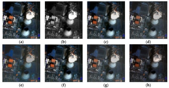
Figure 9. Pansharpening results (source: Pléiades data). (a) Original MS; (b) PAN; (c) the AIHS method; (d) the wavelet method; (e) the PCA method; (f) the EIHS method; (g) the PAIHS method; (h) the MMCMOO method. PAN image resolution is 256 × 256.

Table 2. Results of pansharpening quantitative indicators in Figure 9.

		ERGAS	QAVE	RASE	RMSE	SAM	SID
Reference Value		0	1	0	0	0	0
Figure 9	AIHS	8.3631	0.9246	33.3907	22.9081	2.6158	0.0697
	Wavelet	7.9938	0.9163	31.8892	21.8780	3.7401	0.0696
	PCA	12.0097	0.8552	47.8852	32.852	3.8125	0.0643
	EIHS1 (1000)	4.9393	0.9466	19.7056	13.5193	2.2462	0.0480
	EIHS2 (5000)	4.9020	0.9488	19.5648	13.4227	2.0716	0.056
	EIHS3 (10,000)	3.2076	0.9470	12.7992	8.7810	2.3369	0.0388
	PAIHS1 (100)	2.8285	0.9515	11.2728	7.7339	2.1948	0.0452
	PAIHS5 (300)	2.9351	0.9497	11.6978	8.0254	2.3005	0.0491
	PAIHS6 (500)	2.9351	0.9497	11.6978	8.0254	2.3005	0.0491
	MMCMOO	1.7718	0.9635	7.0693	4.8500	1.5149	0.0319

3.2.2. Comparison and Analysis of Results Obtained from Simulated Data and Real Data

Like other types of data fusion problems, the lack of convincing reference data is a limitation for evaluating fused images. Therefore, in order to solve this problem, this part then applies two evaluation methods in order to make them complement each other. The two methods are as follows.

(1)

The spatial and spectral resolution of the test image is lower than that of the original image MS, and the original image MS is used as a reference;

(2)

No reference image is needed. Compare the difference between the test image and the pansharpened image directly. This method is easy to understand and can be implemented on small-scale data sets.

1)

Simulation data verification

In this section, Google Earth and QuickBird satellite simulation data are used for experimental comparison and analysis. These simulation data mainly cover buildings, roads, trees, vegetation, cars, rivers and other objects collapsed in seismic geological disasters. In this part of the experiment, comparison and analysis will be carried out from multiple angles in order to verify the MMCMOO method in more detail and comprehensively. Figure 10 shows the fused images of Wavelet, PCA, AIHS, EIHS, PAIHS and MMCMOO. The specific analysis is as follows.

Figure 10. Pansharpening results (source: Google Earth). (a) Original MS; (b) PAN; (c) the AIHS method; (d) the wavelet method; (e) the PCA method; (f) the EIHS method; (g) the PAIHS method; (h) the MMCMOO method. PAN image resolution is 256 × 256.

a)

The fused image obtained by the AIHS method can have good spatial quality, but there are some spectral distortions, such as the overall darkening of the image brightness in Figure 10c.

b)

Although the PCA method has good spatial details, it has serious spectral distortion, such as the dim images in Figure 10e, which is the most serious distortion among these methods.

c)

Although the wavelet method reduces the spectral distortion, it produces some aliasing artifacts, such as roads in Figure 10d.

d)

Compared with the AIHS method, the spectral resolution of the fused image obtained by EIHS is better, but the spatial quality still needs to be improved.

e)

The PAIHS method can well preserve the spectral information and spatial structure, but it also produces some ladder effects in smooth areas, such as the blue building area in Figure 10g and the yellow collapsed building area.

MMCMOO, PAIHS and EIHS not only keep the edge of the image clear, but also better reduce blur and blocky artifacts, so as to achieve good results in maintaining spectral information and spatial structure. In contrast, the fusion quality obtained by the proposed MMCMOO method is better than that obtained by the PAIHS and EIHS methods. The car in Figure 10e can reflect these subtle differences.

In addition, Table 3 gives the quantitative results of pansharpening in Figure 10.

Table 3. Results of pansharpening quantitative indicators in Figure 10.

		ERGAS	QAVE	RASE	RMSE	SAM	SID
Reference Value		0	1	0	0	0	0
Figure 10	AIHS	3.9224	0.95191	15.6166	23.9507	2.7416	0.08410
	Wavelet	3.7478	0.85830	14.9068	22.8621	4.2613	0.0993
	PCA	4.6546	0.91414	18.6862	28.6585	2.5035	0.0873
	EIHS	2.4843	0.96839	9.8839	15.1586	1.9190	0.0670
	PAIHS	2.1789	0.96988	8.6727	13.3010	1.8901	0.0695
	MMCMOO	1.7400	0.97513	6.9235	10.6184	1.6184	0.0611

The best values and reference values of the evaluation indexes in the table are shown in bold. In Table 3, the index values obtained by the MMCMOO method are the best among all methods.

2)

Verification of real data

In this section, experiments will be conducted with real data to further prove the effectiveness of the proposed MMCMOO method. Figure 11 and Figure 12 show the fused results of various methods. Table 4 and Table 5 are the quantitative index results corresponding to Figure 11 and Figure 12, respectively. Specific comparison and analysis are as follows.

Figure 11. Comparison of pansharpening results (source: Google Earth). (a) Original MS; (b) PAN; (c) AIHS; (d) Wavelet; (e) PCA; (f) EIHS; (g) PAIHS; (h) MMCMOO. PAN image resolution is 256 × 256.

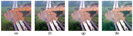
Figure 12. Comparison of pansharpening results (source: QuickBird). (a) Original MS; (b) PAN; (c) the AIHS method; (d) the wavelet method; (e) the PCA method; (f) the EIHS method; (g) the PAIHS method; (h) the MMCMOO method. PAN image resolution is 256 × 256.

Table 4. Results of pansharpening quantitative indicators in Figure 11.

		ERGAS	QAVE	RASE	RMSE	SAM	SID
Reference Value		0	1	0	0	0	0
Figure 11	AIHS	4.1293	0.94097	16.4973	25.4539	2.3498	0.13125
	Wavelet	4.1358	0.80501	16.5123	25.4772	3.9679	0.14411
	PCA	5.8106	0.85143	23.3085	35.9630	3.0627	0.14183
	EIHS	3.8880	0.94651	15.5056	23.9238	2.1764	0.12140
	PAIHS	1.4040	0.94678	5.6097	8.6552	2.8472	0.10405
	MMCMOO	0.9320	0.97462	3.7205	5.7404	1.0968	0.09875

Table 5. Results of pansharpening quantitative indicators in Figure 12.

		ERGAS	QAVE	RASE	RMSE	SAM	SID
Reference Value		0	1	0	0	0	0
Figure 12	AIHS	3.2720	0.93385	13.0914	16.3520	3.1089	0.089752
	Wavelet	3.2293	0.86038	12.8932	16.1044	5.0228	0.084185
	PCA	6.5749	0.83364	26.3658	32.9326	3.7781	0.086307
	EIHS	2.7306	0.94131	10.9116	13.6293	2.6999	0.083147
	PAIHS	2.1474	0.94707	8.5740	10.7095	2.5835	0.081710
	MMCMOO	1.9968	0.95330	7.9779	9.9649	2.1563	0.075920

a)

In Figure 11, it can be found that the wavelet and AIHS methods have some spectral distortion, such as the color of buildings has changed.

b)

The fused images obtained by PCA method have serious contrast distortion, as shown in Figure 11 and Figure 12, where both images are dark.

c)

There is no obvious spectral distortion and spatial distortion in EIHS and PAIHS methods. Overall, the fusion result is relatively good.

d)

Through careful comparison, it is not difficult to find that the fusion images obtained by MMCMOO are clearer and more colorful than those obtained by EIHS and PAIHS, and the fusion effect is better than that obtained by other methods in this paper.

In addition, by analyzing Table 4 and Table 5, it can be found that the comprehensive index values obtained by MMCMOO are the best among all methods. This shows that it has obtained the best spectral quality and spatial quality. Therefore, this part of the experiment once again verified the effectiveness of the MMCMOO method.

3.3. Algorithm Efficiency Analysis

Figure 13 shows the relationship between the quantitative index results of the MMCMOO method and iteration times on the data set of Figure 10. In Figure 13, it can be clearly seen that the MMCMOO method tends to converge when the number of iterations is about 5000. Therefore, in the experiment, setting the value of FES to 5000 is enough to ensure the convergence of the proposed MMCMOO method. In addition, the MMCMOO method is evaluated and analyzed from the point of view of computational efficiency, and the average running time of MMCMOO and other methods on the data sets shown in Figure 10, Figure 11 and Figure 12 is given. See Table 6 for specific data. As we all know, the PCA and Wavelet methods are famous for their computational efficiency, and their running time is much shorter than that of intelligent optimization methods, which is consistent with the data in Table 6. It is also observed that the running time from non-intelligent optimization methods (PCA, Wavelet, AIHS) to intelligent optimization methods (EIHS, PAIHS, MMCMOO) is getting longer. Among them, the execution time of the MMCMOO method is the longest, because its optimization process is the most complicated, and it needs to optimize two objective functions (models) simultaneously. On the whole, although MMCMOO has the longest running time, it has obtained the best fusion quality, so it is still the most competitive fusion method in this paper.

Figure 13. Convergence analysis on different quantitative evaluation metrics.

Table 6. Running time of the various methods (S).

Method	Time
AIHS	0.0528
Wavelet	0.0172
PCA	0.0071
EIHS	88.4305
PAIHS	2024.9153
MMCMOO	8983.5701

3.4. More Discussion

In this section, we will analyze the MMCMOO method from a variety of perspectives and at different levels of analysis. In order to reduce the length of the paper, the following experiments are completed on the representative QuickBird data set.

3.4.1. Model Influence

The primary contribution of the model Z1 is the incorporation of two fidelity terms, one pertaining to spectral information and the other to spatial information. The model Z2 further constrains the fidelity of the spatial resolution of the fused image. Figure 14 shows the difference map of pansharpened images obtained by different models. As illustrated in Figure 14, the difference map generated obtained by model Z1 has the most light spots, bright spots and textures, which means that the model has the most obvious spectral distortion and the most lost spatial information. Although model Z2 can retain the spectral information well, some spatial details are still missing, which is basically consistent with the conclusions of the EIHS and PAIHS methods based on single-objective optimization. The full model in Figure 14, that is, the model proposed in this paper, has the least bright spots and textures in the disparity map, which indicates that the pansharpened image obtained by it has smoother and finer spatial details and more reliable spectral information.

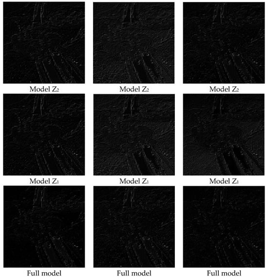
Figure 14. Each row from top to bottom corresponds to optimization Model Z2, Model Z1, and the full model, respectively. From left to right, each column corresponds to the red, green and blue bands, respectively.

3.4.2. Ablation Experiment

Model Z1 is constituted of two distinct energy components. For the sake of simplicity, we may assume that the first half of model Z1 is En(1) and the second half is En(2). In parallel, model Z2 may be designated as En(3). In this section, the influence of each energy division in model Z1 and model Z2 on the fusion results is tested. The experimental results are shown in Figure 15.

Figure 15. Relationship diagram between evaluation index and model selection.

As illustrated in Figure 15, the first term En(1) in model Z1 describes the relationship between panchromatic image P and fused image F, which plays a vital role in the final fusion result. In addition, the second term in model Z1 also has an important influence on the fusion result. If it is abandoned, the final spectral performance will be significantly reduced. Therefore, when selecting the objective function, it is necessary to give consideration to these two energy divisions. It is also noteworthy that although model Z2 has a minimal impact on the MMCMOO indicators (see Figure 15), it is also an indispensable part of the joint model. As can be seen from Figure 15, all the indicators corresponding to the MMCMOO model (Z1+Z2) are the best, which is why Z1 and Z2 are selected as joint models for simultaneous optimization.

4. Conclusions

In this paper, we design and combine two objective functions to propose a new fusion model called MMCMOO, then use the multi-objective optimization algorithm NSGA-II to avoid manual parameter adjustment and to obtain the optimal solution of the two objectives at the same time.

Furthermore, in order to fully verify the superiority of the proposed MMCMOO method, we first verify the feasibility of our method based on experiments with multi-source remote sensing images. Then, simulated data (reduced resolution) and real data (full-scale resolution) are used to quantitatively and qualitatively verify the reliability of the MMCMOO method, respectively. Both from the perspective of modeling and optimization, the evaluation indexes and visual effect comparison show that the proposed MMCMOO is a more reliable and advanced pansharpening method on our datasets.

References

- You, Y.; Wang, R.; Zhou, W. An Optimized Filtering Method of Massive Interferometric SAR Data for Urban Areas by Online Tensor Decomposition. Remote Sens. 2022, 12, 2582. [Google Scholar] [CrossRef]
- Chen, C.; Wang, L.; Zhang, Z.; Lu, C.; Chen, H.; Chen, J. Construction and application of quality evaluation index system for remote-sensing image fusion. J. Appl. Remote Sens. 2022, 16, 012006. [Google Scholar] [CrossRef]
- Zhong, S.; Zhang, Y.; Chen, Y.; Wu, D. Combining Component Substitution and Multiresolution Analysis: A Novel Generalized BDSD Pansharpening Algorithm. IEEE J. Sel. Top. Appl. Earth Obs. Remote Sens. 2017, 10, 2867–2875. [Google Scholar] [CrossRef]
- Liu, P. Pansharpening with transform-based gradient transferring model. IET Image Process. 2019, 13, 2614–2622. [Google Scholar] [CrossRef]
- Yunsong, L.; Jiahui, Q.; Wenqian, D. Hyperspectral Pansharpening via Improved PCA Approach and Optimal Weighted Fusion Strategy. Neurocomputing 2018, 315, 371–380. [Google Scholar]
- Abdolahpoor, A.; Kabiri, P. New texture-based pansharpening method using wavelet packet transform and PCA. Int. J. Wavelets Multiresolution Inf. Process. 2020, 18, 2050025. [Google Scholar] [CrossRef]
- Jin, C.; Deng, L.-J.; Huang, T.-Z.; Vivone, G. Laplacian pyramid networks: A new approach for multispectral pansharpening. Inf. Fusion 2022, 78, 158–170. [Google Scholar] [CrossRef]
- Wady, S.; Bentoutou, Y.; Bengermikh, A.; Bounoua, A.; Taleb, N. A new IHS and wavelet based pansharpening algorithm for high spatial resolution satellite imagery. Adv. Space Res. 2020, 66, 1507–1521. [Google Scholar] [CrossRef]
- Rahmani, S.; Strait, M.; Merkurjev, D. An adaptive IHS pan-sharpening method. IEEE Geosci. Remote Sens. Lett. 2010, 7, 746–750. [Google Scholar] [CrossRef]
- Yilmaz, S. Genetic algorithm-based synthetic variable ratio image fusion. Geocarto Int. 2021, 36, 9–12. [Google Scholar] [CrossRef]
- Wang, T.; Fang, F.; Li, F. High Quality Bayesian Pansharpening. IEEE Trans. Image Process. 2019, 28, 227–239. [Google Scholar] [CrossRef]
- Chen, Y.; Wang, T.; Fang, F.; Zhang, G. A pan-sharpening method based on the ADMM algorithm. Front. Earth Sci. 2019, 13, 656–667. [Google Scholar] [CrossRef]
- Yang, Y.; Lu, H.; Huang, S.; Fang, Y.; Tu, W. An efficient and high-quality pansharpening model based on conditional random fields. Inf. Sci. 2021, 553, 1–18. [Google Scholar] [CrossRef]
- Khateri, M.; Shabanzade, F.; Mirzapour, F. Regularised IHS-based pan-sharpening approach using spectral consistency constraint and total variation. IET Image Process. 2020, 14, 94–104. [Google Scholar] [CrossRef]
- Li, H.; Jing, L. Image fusion framework considering mixed pixels and its application to pansharpening methods based on multiresolution analysis. J. Appl. Remote Sens. 2020, 14, 038501. [Google Scholar] [CrossRef]
- Choi, J.; Park, H.; Seo, D. Pansharpening Using Guided Filtering to Improve the Spatial Clarity of VHR Satellite Imagery. Remote Sens. 2019, 11, 633. [Google Scholar] [CrossRef]
- Chen, Y.; Zhang, G. A Pan-Sharpening Method Based on Evolutionary Optimization and IHS Transformation. Math. Probl. Eng. 2017, 2017, 8269078. [Google Scholar] [CrossRef]
- Huang, W.; Zhang, Y.; Zhang, J.; Zheng, Y. Convolutional Neural Network for Pansharpening with Spatial Structure Enhancement Operator. Remote Sens. 2021, 13, 4062. [Google Scholar] [CrossRef]
- He, L.; Ye, H.; Xi, D.; Zhang, M. Tree-Structured Neural Network for Hyperspectral Pansharpening. IEEE J. Sel. Top. Appl. Earth Obs. Remote Sens. 2024, 17, 2516–2530. [Google Scholar] [CrossRef]
- Guarino, G.; Ciotola, M.; Vivone, G.; Scarpa, G. Band-Wise Hyperspectral Image Pansharpening Using CNN Model Propagation. IEEE Trans. Geosci. Remote Sens. 2024, 62, 1–18. [Google Scholar] [CrossRef]
- Azarang, A.; Kehtarnavaz, N. Application of deep learning models in nonlinear detail map prediction in pansharpening. J. Comput. Sci. 2021, 54, 101431. [Google Scholar] [CrossRef]
- Xie, G.; Nie, R.; Cao, J.; Li, H.; Li, J. A Deep Multiresolution Representation Framework for Pansharpening. IEEE Trans. Geosci. Remote Sens. 2024, 62, 1–16. [Google Scholar] [CrossRef]
- Zhang, J.; Ye, Y.; Fang, F.; Wang, T.; Zhang, G. DMCSC: Deep Multisource Convolutional Sparse Coding Model for Pansharpening. IEEE Trans. Geosci. Remote Sens. 2023, 61, 1–13. [Google Scholar] [CrossRef]
- Li, X.; Li, Y.; Shi, G.; Zhang, L.; Li, W.; Lei, D. Pansharpening Method Based on Deep Nonlocal Unfolding. IEEE Trans. Geosci. Remote Sens. 2023, 61, 1–11. [Google Scholar] [CrossRef]
- Addesso, P.; Conte, R.; Longo, M.; Restaino, R.; Vivone, G. A pansharpening algorithm based on genetic optimization of Morphological Filters. In Proceedings of the IEEE International Geoscience and Remote Sensing Symposium, Munich, Germany, 22–27 July 2012; pp. 5438–5441. [Google Scholar]
- Khademi, G.; Ghassemian, H. A multi-objective component-substitution-based pansharpening. In Proceedings of the 3rd International Conference on Pattern Recognition and Image Analysis (IPRIA), Shahrekord, Iran, 19–20 April 2017; pp. 248–252. [Google Scholar]
- Li, T.; Wang, Y. Biological image fusion using a NSCT based variable-weight method. Inf. Fusion 2011, 12, 85–92. [Google Scholar] [CrossRef]
- Bhatnagar, G.; Wu, Q.M.J.; Liu, Z. Directive Contrast Based Multimodal Medical Image Fusion in NSCT Domain. IEEE Trans. Multimedia 2014, 9, 1014–1024. [Google Scholar] [CrossRef]
- Xie, X.; Xu, Y. Multi-sensor image fusion algorithm based on multi-objective particle swarm optimization algorithm. In Proceedings of the LIDAR Imaging Detection and Target Recognition 2017 Society of Photo-Optical Instrumentation Engineers, Changchun, China, 23–25 July 2017. [Google Scholar]
- Meng, X.; Shen, H.; Li, H.; Zhang, L.; Fu, R. Review of the pansharpening methods for remote sensing images based on the idea of meta-analysis: Practical discussion and challenges. Inf. Fusion 2019, 46, 102–113. [Google Scholar] [CrossRef]
- Zhang, A.; Sun, G.; Wang, Z. Remote sensing imagery classification using multi-objective gravitational search algorithm. In Proceedings of the Image and Signal Processing for Remote Sensing XXII, Edinburgh, UK, 26–29 September 2016; p. 10004. [Google Scholar]
- Wu, X.; Feng, J.; Shang, R.; Zhang, X.; Jiao, L. Multiobjective Guided Divide-and-Conquer Network for Hyperspectral Pansharpening. IEEE Trans. Geosci. Remote Sens. 2022, 60, 1–17. [Google Scholar] [CrossRef]
- Su, X.; Li, J.; Hua, Z. DADR: Dual Attention Based Dual Regression Network for Remote Sensing Image Pan-Sharpening. IEEE J. Sel. Top. Appl. Earth Obs. Remote Sens. 2022, 15, 4397–4413. [Google Scholar] [CrossRef]
- Li, H.; Zhang, Q. Multiobjective Optimization Problems with Complicated Pareto Sets, MOEA/D and NSGA-II. IEEE Trans. Evol. Comput. 2009, 13, 284–302. [Google Scholar] [CrossRef]
- Lin, C.C.; Liu, W.Y.; Peng, Y.C.; Lee, T.K. Altruistic production and distribution planning in the multilayer dual-channel supply chain: Using an improved NSGA-II with lion pride algorithm. Comput. Ind. Eng. 2023, 176, 108884. [Google Scholar] [CrossRef]
- Xie, Y.; Tang, W.; Zhang, F.; Pan, B.; Yue, Y.; Feng, M. Optimization of Variable Blank Holder Force Based on a Sharing Niching RBF Neural Network and an Improved NSGA-II Algorithm. Int. J. Precis. Eng. Manuf. 2019, 20, 285–299. [Google Scholar] [CrossRef]
- Chen, Y.; Liu, C.; Zhou, A. A Multiobjective Pan-sharpening Method for Remote Sensing Images. In Proceedings of the 2019 IEEE Congress on Evolutionary Computation, Wellington, New Zealand, 10–13 June 2019. [Google Scholar]
- Scarpa, G.; Ciotola, M. Full-Resolution Quality Assessment for Pansharpening. Remote Sens. 2022, 14, 1808. [Google Scholar] [CrossRef]
- Masoudi, R.; Kabiri, P. New intensity-hue-saturation pan-sharpening method based on texture analysis and genetic algorithm-adaption. J. Appl. Remote Sens. 2014, 8, 083640. [Google Scholar] [CrossRef]
- Chen, Y.; Chen, Y.; Liu, C. Joint AIHS and particle swarm optimization for Pan-sharpening. Acta Geod. Cartogr. Sin. 2019, 48, 1296–1304. [Google Scholar]
Disclaimer/Publisher’s Note: The statements, opinions and data contained in all publications are solely those of the individual author(s) and contributor(s) and not of MDPI and/or the editor(s). MDPI and/or the editor(s) disclaim responsibility for any injury to people or property resulting from any ideas, methods, instructions or products referred to in the content. |
© 2024 by the authors. Licensee MDPI, Basel, Switzerland. This article is an open access article distributed under the terms and conditions of the Creative Commons Attribution (CC BY) license (https://creativecommons.org/licenses/by/4.0/).