Approximations in Mean Square Analysis of Stochastically Forced Equilibria for Nonlinear Dynamical Systems

Abstract

Motivated by important applications to the analysis of complex noise-induced phenomena, we consider a problem of the constructive description of randomly forced equilibria for nonlinear systems with multiplicative noise. Using the apparatus of the first approximation systems, we construct an approximation of mean square deviations that explicitly takes into account the presence of multiplicative noises, depending on the current system state. A spectral criterion of existence and exponential stability of the stationary second moments for the solution of the first approximation system is presented. For mean square deviation, we derive an expansion in powers of the small parameter of noise intensity. Based on this theory, we derive a new, more accurate approximation of mean square deviations in a general nonlinear system with multiplicative noises. This approximation is compared with the widely used approximation based on the stochastic sensitivity technique. The general mathematical results are illustrated with examples of the model of climate dynamics and the van der Pol oscillator with hard excitement.

1. Introduction

Currently, nonlinear stochastic phenomena such as noise-induced transitions [1,2,3], stochastic excitement [4,5,6,7], noise-induced crisis [8,9], stochastic bifurcations [10,11,12], noise-induced chaos [13,14,15], and stochastic and coherence resonances [16,17,18,19] are being actively studied in various fields of the natural sciences. One of the key mechanisms of such effects is associated with the transition of random trajectories through separatrices detaching basins of coexisting attractors.

In the analysis of such stochastic phenomena, the Monte Carlo method using direct numerical simulation is frequently used [20]. However, in the detailed parametric analysis, this numerical method is extremely time consuming and labor intensive. It is known that a full mathematical description of probability density functions is given by the Kolmogorov–Fokker–Planck Equation [21]. However, even in a two-dimensional case, a direct solution of this equation faces serious mathematical difficulties. In these circumstances, asymptotics and approximations are very useful. Here, asymptotics based on the quasipotential are of particular interest [22,23]. Nowadays, a new geometrical method of confidence domains is used for the approximation of probabilistic distributions. This approach allows one not only to describe the dispersion of random states near the deterministic attractor but also to estimate the critical values of the intensity of random disturbances that generate noise-induced transitions [24,25].

The main idea of this approach is as follows. As the noise intensity increases, the size of the confidence domain increases. The critical value of the noise intensity is found from the condition of the intersection of the confidence domain and the separatrix. The key parameter that determines the configuration of the confidence domain is the stochastic sensitivity of the attractor [26]. Initially, the stochastic sensitivity technique was introduced in connection with the approximation [27] of a quasipotential [22] in the vicinity of an attractor. Currently, this technique has been developed for regular and chaotic attractors of both continuous and discrete systems (see, e.g., [28,29]). The stochastic sensitivity technique and the associated confidence domains method are effectively used in the analysis of nonlinear stochastic phenomena [30,31] and control problems [32,33].

Using the stochastic sensitivity technique, an approximation of the mean square deviations of random states of a stochastic system from the deterministic attractor is constructed. Although formally this technique is applicable to both the case of additive and parametric noise, in the case of parametric noise, the error in the corresponding approximations may be such that the prediction made on the basis of this approximation may turn out to be incorrect.

This paper is devoted to the problem of the approximation of probabilistic distributions of random states around stable equilibria of stochastic differential Ito’s equations with general multiplicative noise. The main contribution of this paper is that we construct an approximation of mean square deviations that explicitly takes into account the impact of multiplicative noises. This more accurate approximation is compared with the previously used approximation based on the stochastic sensitivity technique. The constructive abilities of these general mathematical results are illustrated with examples. For a linear one-dimensional model, we compare two approximations of mean square deviations and derive an explicit formula for the relative error. For a two-dimensional nonlinear climate model, explicit formulas for matrices of mean square deviations are found and compared with the results of a direct numerical simulation. Using a model of a van der Pol oscillator with hard excitement, we show how a new, more accurate approximation makes it possible to predict the occurrence of large-amplitude stochastic oscillations.

2. Mean Square Analysis of Stochastic Equilibria

Consider a nonlinear autonomous system of ordinary differential equations

$$dx=f\left(x\right)dt,$$

(1)

where x is an n-dimensional vector and $f\left(x\right)$ is a sufficiently smooth n-vector function. It is assumed that the system (1) has an exponentially stable equilibrium $\overline{x}$.

Definition 1.

The equilibrium $\overline{x}$ is called exponentially stable in system (1) if for some neighborhood $\mathrm{U}$ of $\overline{x}$ there exist constants $K>0,$$l>0$ such that for all $t⩾0$ it holds that

$$\parallel x\left(t\right)-\overline{x}\parallel ⩽K{e}^{-lt}\parallel x_0-\overline{x}\parallel ,$$

where $x\left(t\right)$ is a solution of the system (1) with the initial condition $x\left(0\right)=x_0\in \mathrm{U}.$ Here, $\parallel ·\parallel$ is the Euclidean norm.

Along with the deterministic system (1), let us consider the stochastic Ito system

$$dx=f\left(x\right)dt+\sum _{i=1}^k{\sigma }_i\left(x\right)d{w}_i\left(t\right),$$

(2)

where ${\sigma }_i\left(x\right)$ are sufficiently smooth n-vector functions and $w_i\left(t\right)$ are scalar standard independent Wiener processes. The functions ${\sigma }_i\left(x\right)$ model the dependence of multiplicative disturbances on the system state. It is worth noting that multiplicative noises are widely studied in systems of different nature, e.g., climate models, ecological systems, biological systems, robotics, financial systems, etc.

Solutions of the stochastic system (2), leaving the deterministic equilibrium $\overline{x}$ under the influence of random disturbances, form some probability distribution. It is assumed that the probabilistic distribution of the states of the system (2) stabilizes. The corresponding stable stationary distribution density satisfies the Fokker–Planck–Kolmogorov Equation [21,22]. It is known that in general cases, it is very difficult to directly use this equation to describe probability distributions, even for two-dimensional systems. Here, the apparatus of the first approximation systems is useful.

2.1. First Approximation System and Its Mean Square Analysis

Let us consider the deviation $z=x-\overline{x}$ of the random state x of the system (2) from the exponentially stable equilibrium $\overline{x}$ of the system (1). The dynamics of the variable z are governed by the following first approximation linear system:

$$dz=Fzdt+\sum _{i=1}^k(S_{0,i}+S_{1,i}z)d{w}_i,$$

(3)

where

$${\displaystyle F=\frac{\partial f}{\partial x}\left(\overline{x}\right),S_{0,i}={\sigma }_i\left(\overline{x}\right),S_{1,i}=\frac{\partial {\sigma }_i}{\partial x}\left(\overline{x}\right).}$$

In our mean square analysis of the system (3) solutions, we will use first (m) and second (M) moments: $m=\mathrm{E}\left(z\right)$, $M=\mathrm{E}(z{z}^{\top })$. The dynamics of these deterministic characteristics are described by the following equations:

$$\dot{m}=Fm,$$

(4)

$$\dot{M}=FM+M{F}^{\top }+\sum _{i=1}^k\left(S_{0,i}{S}_{0,i}^{\top }+S_{0,i}{m}^{\top }{S}_{1,i}^{\top }+S_{1,i}m{S}_{0,i}^{\top }+S_{1,i}M{S}_{1,i}^{\top }\right).$$

(5)

To find an approximation of the dispersion of stationary distributed random states of the nonlinear stochastic system (2) around the deterministic equilibrium $\overline{x}$, we will use the stationary solutions of the system (4), (5).

Due to the exponential stability of the equilibrium $\overline{x}$, it holds that $\mathrm{Re}{\lambda }_i\left(F\right)<0$, where ${\lambda }_i\left(F\right),i=1,...,n,$ are eigenvalues of the matrix F. In these circumstances, the system (4) has a unique stationary stable solution $\overline{m}=0$. Substituting $\overline{m}=0$ into (5), we obtain

$$\dot{M}=FM+M{F}^{\top }+\sum _{i=1}^k\left(S_{0,i}{S}_{0,i}^{\top }+S_{1,i}M{S}_{1,i}^{\top }\right).$$

(6)

So, the matrix $\overline{M}$ of the stationary solution of Equation (6) satisfies the following algebraic equation:

$$F\overline{M}+\overline{M}{F}^{\top }+\sum _{i=1}^k\left(S_{0,i}{S}_{0,i}^{\top }+S_{1,i}\overline{M}{S}_{1,i}^{\top }\right)=0.$$

(7)

Let us consider a deviation $\Delta \left(t\right)=M\left(t\right)-\overline{M}$ where $M\left(t\right)$ is a solution of Equation (6). For the function $\Delta \left(t\right)$, one obtains the homogeneous equation

$$\dot{\Delta }=F\Delta +\Delta F^{\top }+\sum _{i=1}^k{S}_{1,i}\Delta S_{1,i}^{\top }.$$

(8)

The matrix $\Delta \left(t\right)$ is the matrix of second moments $\Delta \left(t\right)=\mathrm{E}y\left(t\right)y{\left(t\right)}^{\top }$ for solutions $y\left(t\right)$ of linear homogeneous stochastic equation

$$dy=Fydt+\sum _{i=1}^k{S}_{1,i}yd{w}_i.$$

(9)

Thus, the question about stability of the stationary solution $\overline{M}$ of Equation (6) is reduced to the equivalent question about the exponential mean square stability of the trivial solution $y=0$ of the stochastic system (9).

Definition 2.

Solution $y\equiv 0$ of the stochastic system (9) is called exponentially stable in mean square, if there exist constants $K>0,$$l>0$ such that for all $t⩾0$ it holds that

$${\mathrm{E}\parallel y\left(t\right)\parallel }^2⩽K{e}^{-lt}\mathrm{E}{\parallel y_0\parallel }^2,$$

where $y\left(t\right)$ is a solution of the system (9) with the initial condition $y\left(0\right)=y_0$.

Let us consider the matrix $S_0={\sum }_{i=1}^k{S}_{0,i}{S}_{0,i}^{\top }$ and operators

$$\mathcal{A}\left[M\right]=FM+M{F}^{\top },\mathcal{S}\left[M\right]=\sum _{i=1}^k{S}_{1,i}M{S}_{1,i}^{\top },\mathcal{P}=-{\mathcal{A}}^{-1}\mathcal{S}.$$

Rewrite Equations (6)–(8) as follows:

$$\dot{M}=\mathcal{A}\left[M\right]+\mathcal{S}\left(M\right)+S_0,$$

(10)

$$\mathcal{A}[\overline{M}]+\mathcal{S}[\overline{M}]+S_0=0,$$

(11)

$$\dot{\Delta }=\mathcal{A}[\Delta ]+\mathcal{S}[\Delta ].$$

(12)

Note that the existence of the operator ${\mathcal{A}}^{-1}$ follows from the condition $\mathrm{Re}{\lambda }_i\left(F\right)<0$.

Basic theoretical connections are presented in the following theorem.

Theorem 1.

The following statements are equivalent:

(a) 

System (10) has a stationary exponentially stable solution $\overline{M}$ satisfying (11);

(b) 

The solution $\Delta \equiv 0$ of the system (12) is exponentially stable;

(c) 

The solution $y\equiv 0$ of the stochastic system (9) is exponentially stable in mean square;

(d) 

It holds that $\mathrm{Re}{\lambda }_i\left(F\right)<0(i=1,...,n)$ and $\rho \left(\mathcal{P}\right)<1$, where $\rho \left(\mathcal{P}\right)$ is the spectral radius of the operator $\mathcal{P}$.

The statements of this theorem were proven or follow from more general results presented in [34,35,36].

Remark 1.

In the one-dimensional case ($n=1$), we have

$$S_0=\sum _{i=1}^k{\sigma }_i^2\left(\overline{x}\right),\mathcal{A}\left[M\right]=2f^{\prime }\left(\overline{x}\right)M,\mathcal{S}\left[M\right]=\sum _{i=1}^k{\left({\sigma }_i^{\prime }\left(\overline{x}\right)\right)}^{2}M,$$

and the condition $\rho \left(\mathcal{P}\right)<1$ has an explicit parametric representation

$$\rho \left(\mathcal{P}\right)=-\frac{1}{2f^{\prime }\left(\overline{x}\right)}\sum _{i=1}^k{\left({\sigma }_i^{\prime }\left(\overline{x}\right)\right)}^2<1.$$

In this case, for the mean square variance of random states around the equilibrium $\overline{x}$, the following estimation can be written

$$M=-\frac{{\sum }_{i=1}^k{\sigma }_i^2\left(\overline{x}\right)}{2f^{\prime }\left(\overline{x}\right)+{\sum }_{i=1}^k{\left({\sigma }_i^{\prime }\left(\overline{x}\right)\right)}^2}.$$

(13)

2.2. Asymptotics for the Case of Weak Noise: Stochastic Sensitivity of the Equilibrium

Consider the stochastic system with weak noises as follows:

$$dx=f\left(x\right)dt+\epsilon \sum _{i=1}^k{\sigma }_i\left(x\right)d{w}_i\left(t\right).$$

(14)

Here, $\epsilon$ is a scalar small parameter of the intensity of random disturbances. For this system, Equation (11) for the covariance matrix M of the equilibrium $\overline{x}$ has the form

$$\mathcal{A}\left[M\right]+{\epsilon }^2\mathcal{S}\left[M\right]+{\epsilon }^2{S}_0=0.$$

(15)

Let us study the dependence of the solution $M\left(\epsilon \right)$ of this equation on the parameter $\epsilon$. Let $W\left(\epsilon \right)$ be the solution to the equation

$$\mathcal{A}\left[W\right]+{\epsilon }^2\mathcal{S}\left[W\right]+S_0=0.$$

(16)

Then $M\left(\epsilon \right)={\epsilon }^{2}W\left(\epsilon \right).$ For $W\left(\epsilon \right)$, one can write the following decomposition:

$$W\left(\epsilon \right)=-{(\mathcal{A}+{\epsilon }^2\mathcal{S})}^{-1}\left[S_0\right]=-{\left(I+{\epsilon }^2{\mathcal{A}}^{-1}\mathcal{S}\right)}^{-1}{\mathcal{A}}^{-1}\left[S_0\right]=$$

$$={\left(I-{\epsilon }^2\mathcal{P}\right)}^{-1}\left[W\left(0\right)\right].$$

For small $\epsilon$, it holds that

$$W\left(\epsilon \right)=\sum _{m=0}^{\infty }{\epsilon }^{2m}{\mathcal{P}}^m\left[W\left(0\right)\right]=W\left(0\right)+{\epsilon }^2\mathcal{P}\left[W\left(0\right)\right]+{\epsilon }^4{\mathcal{P}}^2\left[W\left(0\right)\right]+...$$

As a result, for the matrix function $M\left(\epsilon \right)$ we obtain the expansion in powers of the small parameter, as follows:

$$M\left(\epsilon \right)=\sum _{m=0}^{\infty }{\epsilon }^{2m+2}{\mathcal{P}}^m\left[W\left(0\right)\right]={\epsilon }^{2}W\left(0\right)+{\epsilon }^4\mathcal{P}\left[W\left(0\right)\right]+{\epsilon }^6{\mathcal{P}}^2\left[W\left(0\right)\right]...$$

(17)

In this series, the matrix $W\left(0\right)$ plays an important role in the asymptotic analysis of the dispersion of random states around the equilibrium. Because of $W\left(0\right)={lim}_{\epsilon \to 0}\frac{1}{{\epsilon }^2}M\left(\epsilon \right)$, this matrix characterizes the stochastic sensitivity of the equilibrium [26] to the impact of weak noise. Thus, in the first approximation, we have

$$M\left(\epsilon \right)\approx M^{\left(1\right)}\left(\epsilon \right)={\epsilon }^{2}W,$$

(18)

where W is a solution of the following equation

$$FW+W{F}^{\top }+S_0=0.$$

(19)

If the noise in the system (14) does not depend on the state, then $\mathcal{P}=0$ and the first approximation coincides with the exact value $M\left(\epsilon \right)={\epsilon }^{2}W.$ In general, using W as an approximation for $M\left(\epsilon \right)$, one obtains an underestimation of the covariance of random states. Indeed, since the operator $\mathcal{P}$ is positive [37], the inequality $M\left(\epsilon \right)⪰{\epsilon }^{2}W$ is valid.

In a one-dimensional case, the stochastic sensitivity of the equilibrium $\overline{x}$ for the system (14) is given by the formula

$$W=-\frac{{\sum }_{i=1}^k{\sigma }_i^2\left(\overline{x}\right)}{2f^{\prime }\left(\overline{x}\right)}.$$

(20)

3. Examples

Let us consider how these theoretical results can be applied to the approximation of mean square deviation of random states from the equilibrium in some stochastic systems.

Example 1.

Consider a simple one-dimensional stochastic system

$$dx=-axdt+\epsilon ({\sigma }_{1}d{w}_1\left(t\right)+{\sigma }_{2}xd{w}_2\left(t\right)),$$

where $a,{\sigma }_1,$ and ${\sigma }_2$ are non-negative parameters, ε is the intensity of random disturbances, $w_i\left(t\right)$ are uncorrelated scalar Wiener processes. The parameters ${\sigma }_1$ and ${\sigma }_2$ specify the weights of additive and multiplicative disturbances, accordingly.

For $a>0$, the corresponding deterministic system (with $\epsilon =0$) has an exponentially stable equilibrium $\overline{x}=0.$ Second moments $M\left(t\right)=\mathrm{E}{(x\left(t\right)-\overline{x})}^2$ of deviations of solutions $x\left(t\right)$ from the equilibrium satisfy the equation

$$\dot{M}=-2aM+{\epsilon }^2({\sigma }_1^2+{\sigma }_2^{2}M).$$

This equation has a stationary solution

$$M\left(\epsilon \right)=\frac{{\epsilon }^2{\sigma }_1^2}{2a-{\epsilon }^2{\sigma }_2^2}.$$

Following the decomposition (17), for weak noise, $M\left(\epsilon \right)$ has the following asymptotics:

$$M\left(\epsilon \right)={\epsilon }^{2}W+O\left({\epsilon }^4\right),$$

where W characterizes the stochastic sensitivity of the equilibrium $\overline{x}$. Here, W satisfies (see (19)) the equation:

$$-2aW+{\sigma }_1^2=0.$$

Using W, one can write the first approximation for the function $M\left(\epsilon \right)$:

$$M^{\left(1\right)}\left(\epsilon \right)={\epsilon }^{2}W=\frac{{\epsilon }^2{\sigma }_1^2}{2a}.$$

Formally, the approximation $M^{\left(1\right)}\left(\epsilon \right)$ is defined for any $a>0$ while the approximated function $M\left(\epsilon \right)$ is defined only for $a>\frac{{\epsilon }^2{\sigma }_2^2}{2}.$ In absence of multiplicative noise $({\sigma }_2=0$), the values $M^{\left(1\right)}$ and M are identical. At ${\sigma }_2\ne 0$, they can essentially differ.

This difference is clearly seen in Figure 1 where plots of the functions M (solid line) and $M^{\left(1\right)}$ (dashed line) are shown versus parameter a. Note that the approximation $M^{\left(1\right)}$ is always less than M (this fact was shown above for the general case). Moreover, in the interval $0<a<\frac{{\epsilon }^2{\sigma }_2^2}{2},$ where the approximation gives finite values, the original function is not defined at all: the second moments $M\left(t\right)$ tend to infinity. In the interval $a>\frac{{\epsilon }^2{\sigma }_2^2}{2}$, the approximation error monotonically increases and tends to infinity as it approaches the bifurcation value $a_{*}=\frac{{\epsilon }^2{\sigma }_2^2}{2}$. For the relative error, an explicit representation can be written as follows:

$$\left|\frac{M-M^{\left(1\right)}}{M}\right|=\frac{{\epsilon }^2{\sigma }_2^2}{2a}.$$

Let us continue the comparison of these two methods for estimating the dispersion of random states around the equilibrium using the two-dimensional systems as examples.

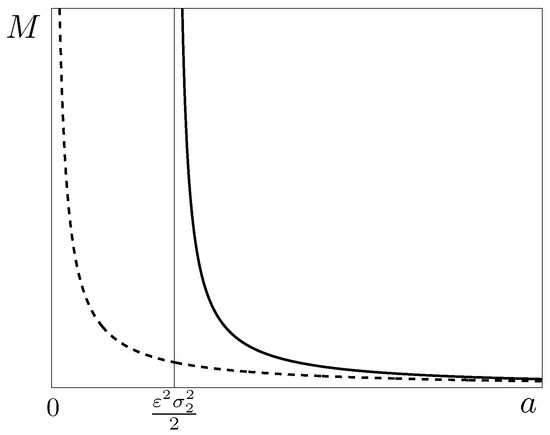
Figure 1. Stationary second moments M (solid line) and approximation $M^{\left(1\right)}$ (dashed) versus parameter a.

Example 2.

Consider a stochastic version of the two-dimensional model [38] of climate dynamics:

$$\begin{array}{c}dx=(y-x)dt\hfill \\ dy=(-ax+by-x^{2}y)dt+\epsilon ({\sigma }_{1}d{w}_1+{\sigma }_{2}yd{w}_2).\hfill \end{array}$$

(21)

Here, the variable x describes the marine ice latitude, y stands for the ocean temperature. In model (21), ${\sigma }_1$ and ${\sigma }_2$ characterize intensities of the additive and multiplicative noises, respectively, $w_1\left(t\right),w_2\left(t\right)$ are scalar standard independent Wiener processes, and ε is the small parameter. The deterministic system (21) (with $\epsilon =0$ therein) has the equilibrium $E(0,0)$. For this equilibrium, the Jacobi matrix is

$$F=\left[\begin{array}{cc}-1& 1\\ -a& b\end{array}\right].$$

The equilibrium $E(0,0)$ is exponentially stable if $b<1$ and $b<a.$

As it follows from the theory presented above, the covariance matrix $M=\left[\begin{array}{cc}{m}_{11}& m_{12}\\ m_{21}& m_{22}\end{array}\right]$ of random states of the stochastic climate model (21) near the equilibrium $E(0,0)$ satisfies Equation (15), where

$$\mathcal{S}\left[M\right]=\left[\begin{array}{cc}0& 0\\ 0& {\sigma }_2^2{m}_{22}\end{array}\right],S_0=\left[\begin{array}{cc}0& 0\\ 0& {\sigma }_1^2\end{array}\right].$$

For elements of the symmetric matrix M, the following system can be written as follows:

$$\left\{\begin{array}{c}-2m_{11}+2m_{12}=0,\hfill \\ -a{m}_{11}+(b-1)m_{12}+m_{22}=0,\hfill \\ -2a{m}_{12}+2b{m}_{22}+{\epsilon }^2{\sigma }_2^2{m}_{22}+{\epsilon }^2{\sigma }_1^2=0.\hfill \end{array}\right.$$

This system has an explicit solution, as follows:

$$m_{11}=m_{12}=\frac{{\epsilon }^2{\sigma }_1^2}{2a+(2b+{\epsilon }^2{\sigma }_2^2)(b-a-1)},m_{22}=\frac{{\epsilon }^2{\sigma }_1^2(a+1-b)}{2a+(2b+{\epsilon }^2{\sigma }_2^2)(b-a-1)}.$$

(22)

The first approximation matrix $M^{\left(1\right)}$ from (18) for the model (21) has elements

$$m_{11}^{\left(1\right)}=m_{12}^{\left(1\right)}=\frac{{\epsilon }^2{\sigma }_1^2}{2a+2b(b-a-1)},m_{22}^{\left(1\right)}=\frac{{\epsilon }^2{\sigma }_1^2(a+1-b)}{2a+2b(b-a-1)}.$$

(23)

The accuracy of the approximation M and $M^{\left(1\right)}$ can be seen in Figure 2. Here, for the fixed values $a=1,b=0.9,{\sigma }_1=0.1,{\sigma }_2=10$, mean square deviations $\mathrm{E}(x^2)$ and $\mathrm{E}(y^2)$ (asterisks) were calculated via direct numerical simulation of solutions of the nonlinear stochastic model (21). Approximations $m_{11}\left(\epsilon \right)$ and $m_{22}\left(\epsilon \right)$ found from (22) are plotted here by solid lines, and approximations $m_{11}^{\left(1\right)}\left(\epsilon \right)$ and $m_{22}^{\left(1\right)}\left(\epsilon \right)$ found from (23) are plotted by dashed lines. As can be seen, $m_{11}\left(\epsilon \right)$ and $m_{22}\left(\epsilon \right)$ agree well with results of direct numerical simulations while $m_{11}^{\left(1\right)}\left(\epsilon \right)$ and $m_{22}^{\left(1\right)}\left(\epsilon \right)$ significantly underestimate $\mathrm{E}(x^2)$ and $\mathrm{E}(y^2)$.

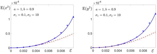
Figure 2. Stochastic system (21) with $a=1,b=0.9,{\sigma }_1=0.1,{\sigma }_2=10$. Here, mean square deviations $\mathrm{E}\left(x^2\right)$ (left) and $\mathrm{E}\left(y^2\right)$ (right) calculated via the direct numerical simulation of system (21) solutions for different $\epsilon$ are shown by asterisks. Approximations $m_{11}\left(\epsilon \right)$ (left) and $m_{22}\left(\epsilon \right)$ (right) are plotted by solid curves. Approximations $m_{11}^{\left(1\right)}\left(\epsilon \right)$ (left) and $m_{22}^{\left(1\right)}\left(\epsilon \right)$ (right) are plotted by dashed curves.

Example 3.

Consider the van der Pol model with hard excitation of self-oscillations, as follows:

$$\begin{array}{c}dx=ydt\hfill \\ dy=(-x+(a+b{x}^2-x^4)y)dt+{\sigma }_{1}d{w}_1+{\sigma }_{2}yd{w}_2.\hfill \end{array}$$

(24)

Here, ${\sigma }_1$ is the intensity of the additive noise, ${\sigma }_2$ is the intensity of the multiplicative noise, and $w_1\left(t\right),w_2\left(t\right)$ are scalar standard independent Wiener processes.

Let us fix $a=-0.1,b=2$. For this set of parameters, the deterministic system (24) with ${\sigma }_1={\sigma }_2=0$ is bistable and exhibits the coexisting attractors: the stable equilibrium $\overline{x}=0,$$\overline{y}=0$ and stable limit cycle. Basins of these attractors are separated by the orbit of the unstable limit cycle. In Figure 3a and Figure 4a, the equilibrium is shown by a black filled circle, the stable cycle is plotted by a blue curve, and the unstable cycle (the separatrix) is shown by a red curve.

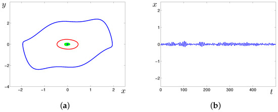
Figure 3. Stochastic system (24) with ${\sigma }_1=0.02,{\sigma }_2=0.2$: (a) random trajectory (green) of the solution starting at the equilibrium $(0,0)$; (b) time series.

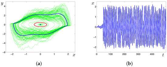
Figure 4. Stochastic system (24) with ${\sigma }_1=0.05,{\sigma }_2=0.4$: (a) random trajectory (green) of the solution starting at the equilibrium $(0,0)$; (b) time series.

Let us consider the behavior of trajectories of the stochastic system (24) solutions starting at the equilibrium $(0,0)$. Under the influence of weak random disturbances, trajectories leave the stable equilibrium and form a stationary probability distribution concentrated in a small neighborhood of the origin. These types of dynamics correspond to the unexcited mode of the oscillator (see Figure 3 for ${\sigma }_1=0.02,{\sigma }_2=0.2$).

As the noise intensity increases, random trajectories cross the separatrix (unstable limit cycle) and continue to oscillate near the stable cycle. This means a transition to the excitation mode (see Figure 3 for ${\sigma }_1=0.05,{\sigma }_2=0.4$).

For the analytical approximation of the dispersion of random states, we will use the theory presented above.

For system (24), the parameters of Equation (7) are as follow:

$$F=\left[\begin{array}{cc}0& 1\\ -1& a\end{array}\right],M=\left[\begin{array}{cc}{m}_{11}& m_{12}\\ m_{21}& m_{22}\end{array}\right],$$

$$S_{0,1}={\sigma }_1\left[\begin{array}{c}0\\ 1\end{array}\right],S_{0,2}=\left[\begin{array}{c}0\\ 0\end{array}\right],S_{1,1}=\left[\begin{array}{cc}0& 0\\ 0& 0\end{array}\right],S_{1,2}={\sigma }_2\left[\begin{array}{cc}0& 0\\ 0& 1\end{array}\right].$$

Now, we can write the matrix Equation (7) as the following system for the elements $m_{ij}$ of the symmetric matrix M:

$$-m_{11}+a{m}_{12}+m_{22}=0,m_{12}=m_{21}=0,-2m_{12}+2a{m}_{22}+{\sigma }_1^2+{\sigma }_2^2{m}_{22}=0.$$

From this system, we have solution

$$m_{11}=m_{22}=-\frac{{\sigma }_1^2}{2a+{\sigma }_2^2},m_{12}=m_{21}=0.$$

Thus, the matrix M that defines mean square deviation of random states from the equilibrium $(0,0)$ is

$$M=-\frac{{\sigma }_1^2}{2a+{\sigma }_2^2}\left[\begin{array}{cc}1& 0\\ 0& 1\end{array}\right].$$

Note that the asymptotic method of stochastic sensitivity gives for mean square deviation another approximation, as follows:

$$M^{\left(1\right)}=-\frac{{\sigma }_1^2}{2a}\left[\begin{array}{cc}1& 0\\ 0& 1\end{array}\right].$$

The difference in these approximations can lead to qualitative differences in the prediction of the results of the noise influence. Let us consider how these two estimations work in the context of the confidence domains method. For diagonal $2\times 2$ matrices, the equation of the confidence ellipse is written as

$$\frac{x^2}{m_{11}}+\frac{y^2}{m_{22}}=-2ln(1-P).$$

Here, P is fiducial probability.

Confidence ellipses are effectively used in predicting noise-induced transitions through the separatrix. Figure 5 shows two confidence ellipses constructed using the matrices M (larger ellipse) and $M^{\left(1\right)}$ (smaller ellipse) for the stochastic system (24) with $a=-1,{\sigma }_1=0.05,{\sigma }_2=0.4.$ The larger ellipse captures the basin of attraction of the limit cycle, which allows us to make a prediction about the generation of large-amplitude oscillations (excitation mode). The smaller ellipse is entirely contained in the basin of attraction of the stable equilibrium and therefore predicts the unexcited mode of the oscillator. As we see, an error in estimating the second moments can lead to qualitative errors in solving important prediction problems. Note that this prediction agrees well with the results of direct numerical simulations (compare Figure 3, Figure 4 and Figure 5).

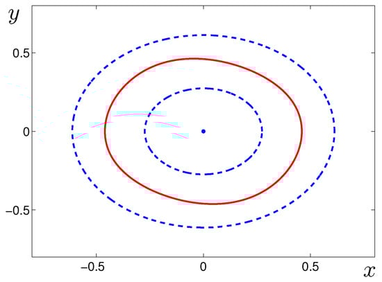
Figure 5. Confidence ellipses (dashed) and unstable cycle (red solid) for the system (24) with $a=-1,{\sigma }_1=0.05,{\sigma }_2=0.4$. The internal ellipse is constructed using the matrix $M^{\left(1\right)}$, and the external ellipse is constructed using the matrix M. Here, fiducial probability $P=0.99$.

4. Conclusions

This paper is devoted to the problem of approximating probability distributions of random states near the equilibrium of the stochastic system with multiplicative noise. The system of nonlinear stochastic differential Ito’s equations is used as a basic mathematical model. For a solution of the linear first approximation system, we present an algebraic criterion of existence and exponential stability of the stationary second moments. For mean square deviation, an expansion in powers of the small parameter of noise intensity is derived. Using this mathematical theory, we derive a new, more accurate approximation of mean square deviations in a general nonlinear system with multiplicative noises. This approximation is compared with the widely used approximation based on the stochastic sensitivity technique. The general mathematical results are applied to examples. For the climate model, explicit formulas for matrices of mean square deviations are derived and compared with the results of direct numerical simulation. For the van der Pol oscillator with hard excitement, it is shown that using the elaborated more accurate approximation, one can predict the onset of noise-induced generation of large-amplitude stochastic oscillations. This prediction agrees well with the results of direct numerical simulations. It is worth noting that extending the more accurate approximation obtained here for equilibrium to the more complex cases of limit cycles and chaotic attractors is an attractive challenge.

References

- Horsthemke, W.; Lefever, R. Noise-Induced Transitions; Springer: Berlin, Germany, 1984; p. 338. [Google Scholar]
- Anishchenko, V.S.; Astakhov, V.V.; Neiman, A.B.; Vadivasova, T.E.; Schimansky-Geier, L. Nonlinear Dynamics of Chaotic and Stochastic Systems. Tutorial and Modern Development; Springer: Berlin/Heidelberg, Germany, 2007; p. 535. [Google Scholar]
- Ducimetiére, Y.M.; Boujo, E.; Gallaire, F. Noise-induced transitions past the onset of a steady symmetry-breaking bifurcation: The case of the sudden expansion. Phys. Rev. Fluids 2024, 9, 053905. [Google Scholar] [CrossRef]
- Lindner, B.; Garcia-Ojalvo, J.; Neiman, A.; Schimansky-Geier, L. Effects of noise in excitable systems. Phys. Rep. 2004, 392, 321–424. [Google Scholar] [CrossRef]
- Chen, Z.; Zhu, J. Non-differentiability of quasi-potential and non-smooth dynamics of optimal paths in the stochastic Morris-Lecar model: Type I and II excitability. Nonlinear Dyn. 2019, 96, 2293–2305. [Google Scholar] [CrossRef]
- Lima Dias Pinto, I.; Copelli, M. Oscillations and collective excitability in a model of stochastic neurons under excitatory and inhibitory coupling. Phys. Rev. E 2019, 100, 062416. [Google Scholar] [CrossRef] [PubMed]
- Ryashko, L. Analysis of excitement caused by colored noise in a thermokinetic model. Mathematics 2023, 11, 4676. [Google Scholar] [CrossRef]
- Anishchenko, V.S.; Khairulin, M.E. Effect of noise-induced crisis of attractor on characteristics of Poincaré recurrence. Tech. Phys. Lett. 2011, 37, 561–564. [Google Scholar] [CrossRef]
- Cisternas, J.; Descalzi, O. Intermittent explosions of dissipative solitons and noise-induced crisis. Phys. Rev. E 2013, 88, 022903. [Google Scholar] [CrossRef] [PubMed]
- Arnold, L. Random Dynamical Systems; Springer: Berlin, Germany, 1998; p. 600. [Google Scholar]
- Zakharova, A.; Kurths, J.; Vadivasova, T.; Koseska, A. Analysing dynamical behavior of cellular networks via stochastic bifurcations. PLoS ONE 2011, 6, e19696. [Google Scholar] [CrossRef] [PubMed][Green Version]
- Jin, C.; Sun, Z.; Xu, W. A novel stochastic bifurcation and its discrimination. Commun. Nonlinear Sci. Numer. Simul. 2022, 110, 106364. [Google Scholar] [CrossRef]
- Gao, J.B.; Hwang, S.K.; Liu, J.M. When can noise induce chaos? Phys. Rev. Lett. 1999, 82, 1132–1135. [Google Scholar] [CrossRef]
- Lai, Y.C.; Tel, T. Transient Chaos. Complex Dynamics on Finite Time Scales; Springer: New York, NY, USA, 2011; p. 502. [Google Scholar]
- Agarwal, V.; Yorke, J.; Balachandran, B. Noise-induced chaotic-attractor escape route. Nonlinear Dyn. 2020, 102, 863–876. [Google Scholar] [CrossRef]
- Pikovsky, A.S.; Kurths, J. Coherence resonance in a noise-driven excitable system. Phys. Rev. Lett. 1997, 78, 775–778. [Google Scholar] [CrossRef]
- Schmid, G.; Hänggi, P. Intrinsic coherence resonance in excitable membrane patches. Math. Biosci. 2007, 207, 235–245. [Google Scholar] [CrossRef] [PubMed][Green Version]
- McDonnell, M.D.; Stocks, N.G.; Pearce, C.E.M.; Abbott, D. Stochastic Resonance: From Suprathreshold Stochastic Resonance to Stochastic Signal Quantization; Cambridge University Press: Cambridge, UK, 2008; p. 446. [Google Scholar]
- Palabas, T.; Torres, J.J.; Perc, M.; Uzuntarla, M. Double stochastic resonance in neuronal dynamics due to astrocytes. Chaos Solitons Fractals 2023, 168, 113140. [Google Scholar] [CrossRef]
- Kloeden, P.E.; Platen, E. Numerical Solution of Stochastic Differential Equations; Springer: Berlin, Germany, 1992; p. 636. [Google Scholar]
- Risken, H. The Fokker–Planck Equation: Methods of Solution and Applications; Springer: Berlin, Germany, 1984. [Google Scholar]
- Freidlin, M.I.; Wentzell, A.D. Random Perturbations of Dynamical Systems; Springer: New York, NY, USA, 1984. [Google Scholar]
- Li, Y.; Xu, S.; Duan, J.; Liu, X.; Chu, Y. A machine learning method for computing quasi-potential of stochastic dynamical systems. Nonlinear Dyn. 2022, 109, 1877–1886. [Google Scholar] [CrossRef]
- Xu, C.; Yuan, S.; Zhang, T. Confidence domain in the stochastic competition chemostat model with feedback control. Appl. Math. J. Chin. Univ. 2018, 33, 379–389. [Google Scholar] [CrossRef]
- Ryashko, L. Sensitivity analysis of the noise-induced oscillatory multistability in Higgins model of glycolysis. Chaos 2018, 28, 033602. [Google Scholar] [CrossRef] [PubMed]
- Bashkirtseva, I. Stochastic sensitivity analysis: Theory and numerical algorithms. IOP Conf. Ser. Mater. Sci. Eng. 2017, 192, 012024. [Google Scholar] [CrossRef]
- Mil’shtein, G.; Ryashko, L. A first approximation of the quasipotential in problems of the stability of systems with random non-degenerate perturbations. J. Appl. Math. Mech. 1995, 59, 47–56. [Google Scholar] [CrossRef]
- Sun, Y.; Hong, L.; Jiang, J. Stochastic sensitivity analysis of nonautonomous nonlinear systems subjected to Poisson white noise. Chaos Solitons Fractals 2017, 104, 508–515. [Google Scholar] [CrossRef]
- Bashkirtseva, I.; Ryashko, L. Stochastic sensitivity analysis of chaotic attractors in 2D non-invertible maps. Chaos Solitons Fractals 2019, 126, 78–84. [Google Scholar] [CrossRef]
- Alexandrov, D.V.; Bashkirtseva, I.A.; Crucifix, M.; Ryashko, L.B. Nonlinear climate dynamics: From deterministic behaviour to stochastic excitability and chaos. Phys. Rep. 2021, 902, 1–60. [Google Scholar] [CrossRef]
- Garain, K.; Sarathi Mandal, P. Stochastic sensitivity analysis and early warning signals of critical transitions in a tri-stable prey-predator system with noise. Chaos 2022, 32, 033115. [Google Scholar] [CrossRef] [PubMed]
- Bashkirtseva, I.; Ryashko, L.; Chen, G. Stochastic sensitivity synthesis in nonlinear systems with incomplete information. J. Frankl. Inst. 2020, 357, 5187–5198. [Google Scholar] [CrossRef]
- Huang, M.; Yang, A.; Yuan, S.; Zhang, T. Stochastic sensitivity analysis and feedback control of noise-induced transitions in a predator-prey model with anti-predator behavior. Math. Biosci. Eng. 2023, 20, 4219–4242. [Google Scholar] [CrossRef] [PubMed]
- Ryashko, L. Stabilization of linear stochastic systems with state and control dependent perturbations. J. Appl. Math. Mech. 1981, 43, 655–663. [Google Scholar] [CrossRef]
- Mao, X. Exponential Stability of Stochastic Differential Equations; Marcel Dekker: New York, NY, USA, 1994; p. 307. [Google Scholar]
- Khasminskii, R. Stochastic Stability of Differential Equations; Springer: Berlin, Germany, 2012. [Google Scholar]
- Krasnosel’skij, M.A.; Lifshits, J.A.; Sobolev, A.V. Positive Linear Systems, the Method of Positive Operators; Heldermann Verlag: Berlin, Germany, 1989; p. 354. [Google Scholar]
- Saltzman, B.; Sutera, A.; Evenson, A. Structural stochastic stability of a simple auto-oscillatory climatic feedback system. J. Athmospheric Sci. 1981, 38, 494–503. [Google Scholar] [CrossRef]
Disclaimer/Publisher’s Note: The statements, opinions and data contained in all publications are solely those of the individual author(s) and contributor(s) and not of MDPI and/or the editor(s). MDPI and/or the editor(s) disclaim responsibility for any injury to people or property resulting from any ideas, methods, instructions or products referred to in the content. |
© 2024 by the author. Licensee MDPI, Basel, Switzerland. This article is an open access article distributed under the terms and conditions of the Creative Commons Attribution (CC BY) license (https://creativecommons.org/licenses/by/4.0/).