
A Modified Sand Cat Swarm Optimization Algorithm Based on Multi-Strategy Fusion and Its Application in Engineering Problems

Abstract
1. Introduction
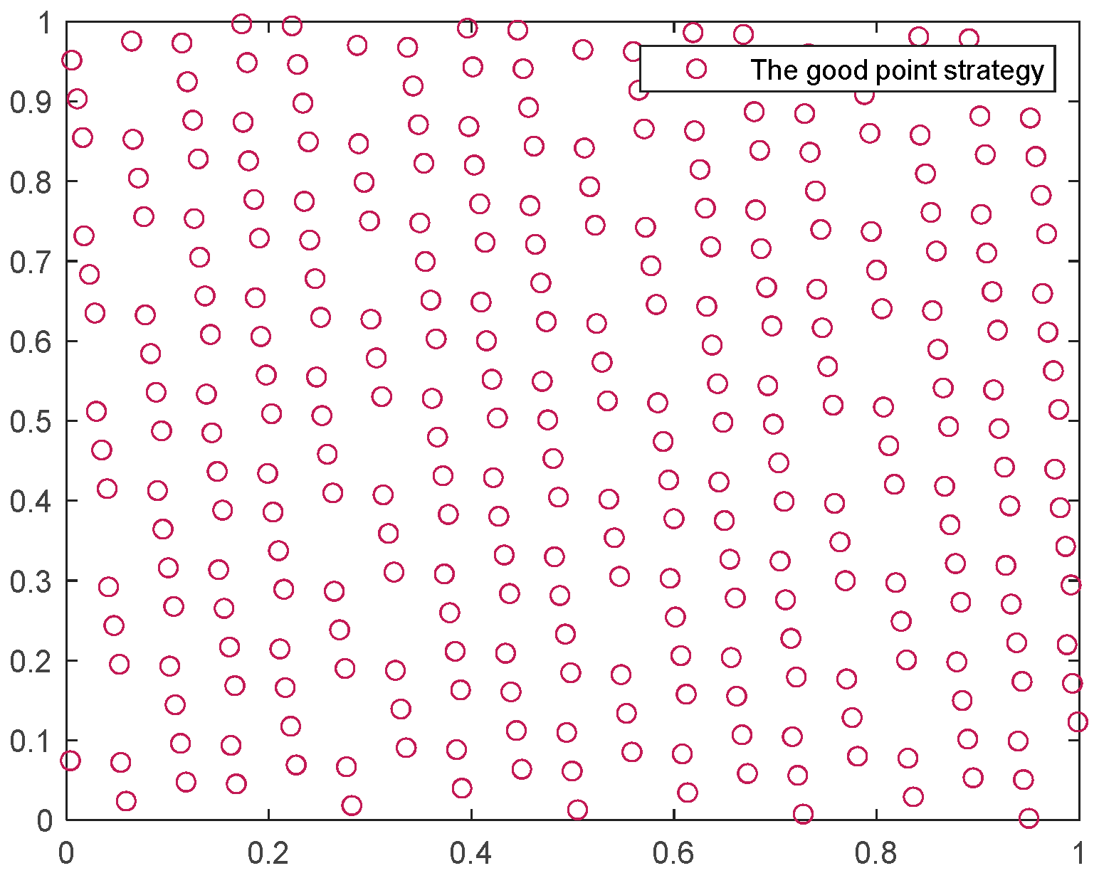
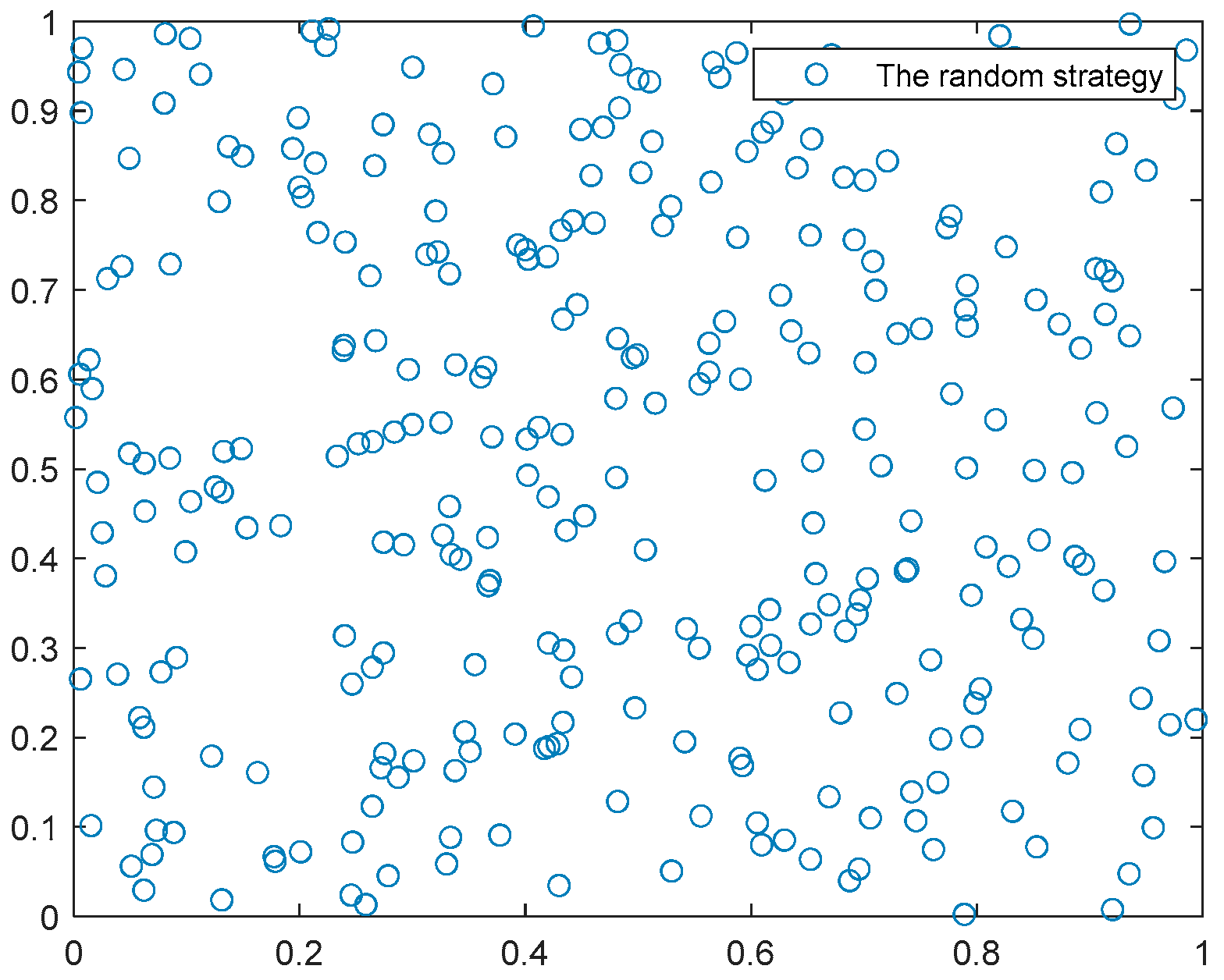
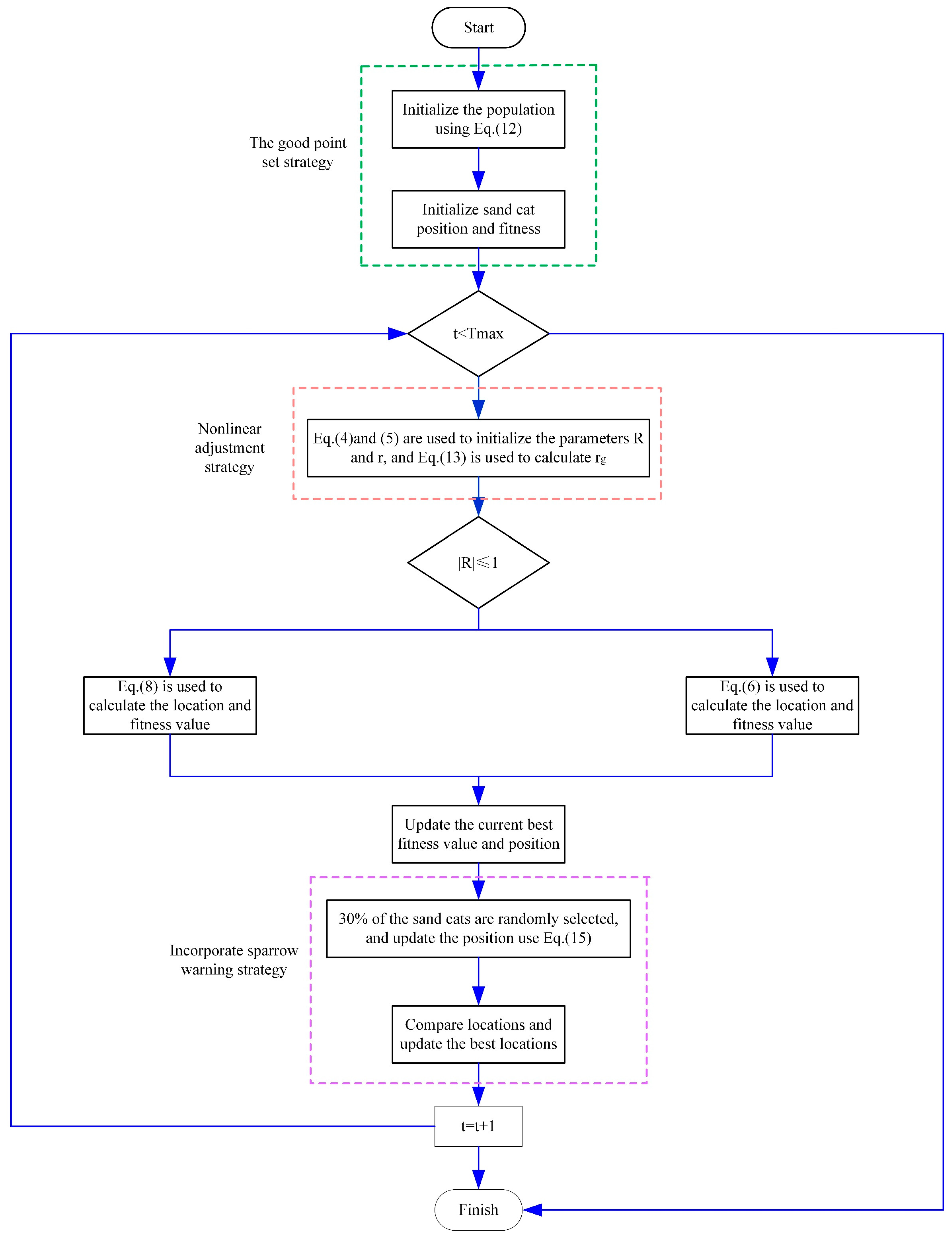
- During the initial population phase, the good point set strategy is adopted to ensure the population is evenly distributed within the search space, enhancing population diversity.
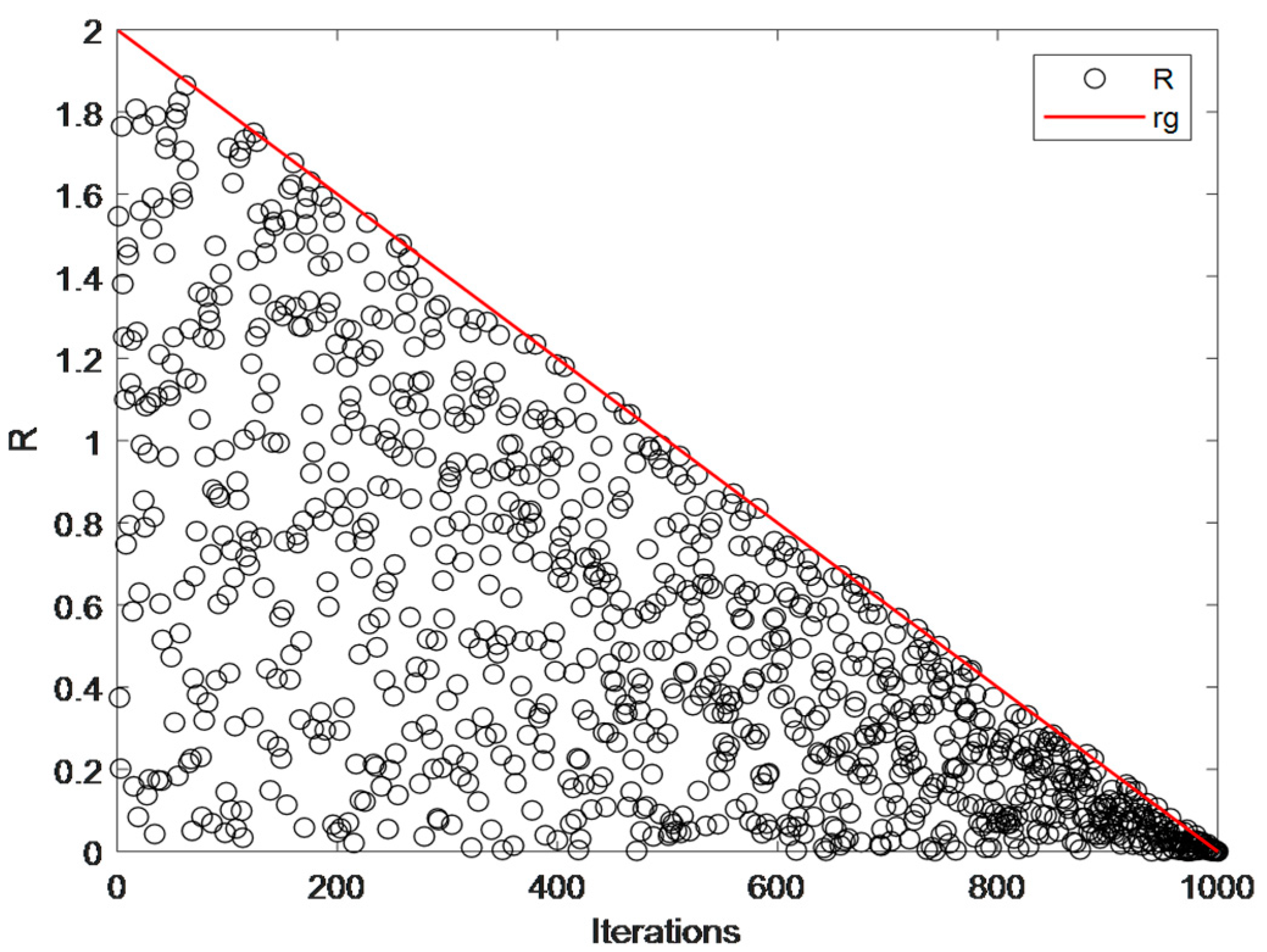
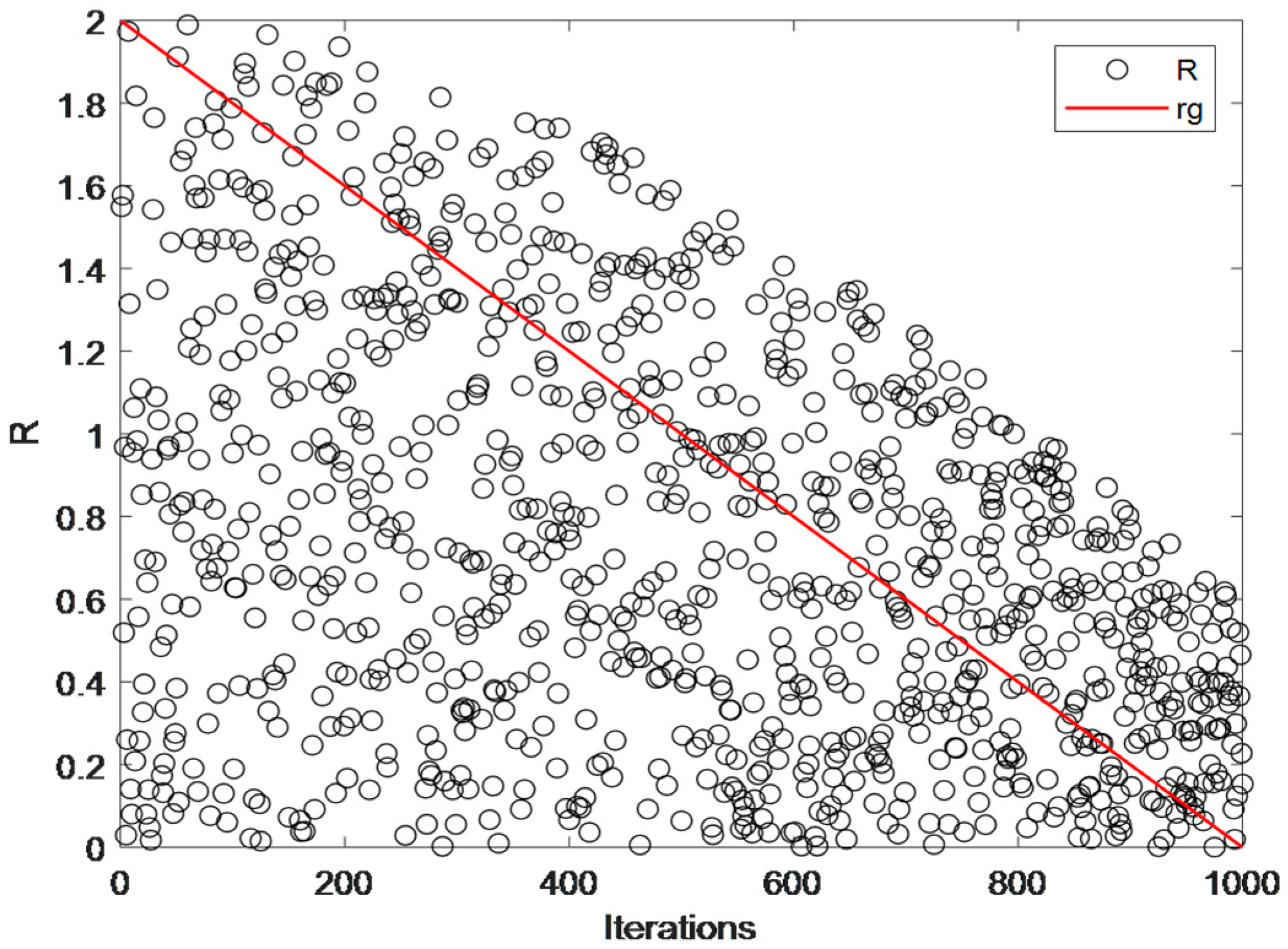
- A nonlinear adjustment strategy is introduced in the exploration phase to improve the sand cat’s sensitivity range, dynamically adjusting the balance conversion parameters between the exploration and exploitation stages.it expands the search range of the sand cats, enhances the algorithm’s global search ability, and reduces the risk of falling into local optima.
- In the exploitation phase, the sparrow search algorithm’s warning mechanism is fused to update the sand cats’ positions, enabling them to respond quickly when approaching optimality, avoid falling into local optima, and accelerate the algorithm’s convergence speed.
2. SCSO: Sand Cat Swarm Optimization Algorithm
2.1. Population Initialization
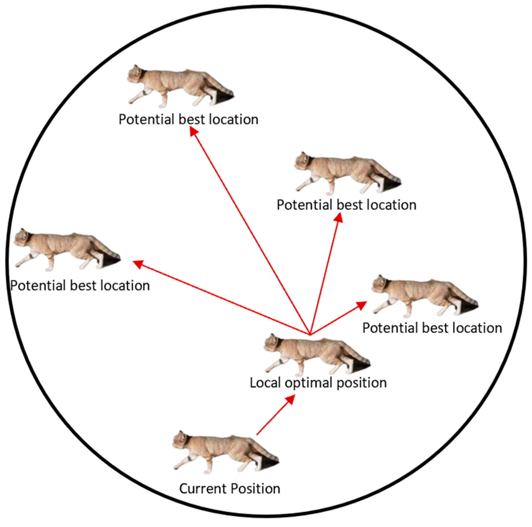
2.2. Search for Prey (Exploration Phase)
2.3. Attacking Prey (Development Phase)
| Algorithm 1 SCSO |
| 1: Initialize the population |
| 2: Calculate the fitness function based on the objective function |
| 3: Use Equations (3)–(5) to initialize the parameters , R, and r |
| 4: while (t < T) do |
| 5: for Every individual do |
| 6: Take a random angle θ between 0 and 360° |
| 7: if |R| ≤ 1 |
| 8: Use Equation (8) to update the position |
| 9: else |
| 10: Use Equation (6) to update the location |
| 11: end |
| 12: end |
| 13: end |
3. MSCSO: Fusion of Multi-Strategy Sand Cat Swarm Optimization Algorithm
3.1. The Good Point Set Strategy
3.2. Nonlinear Adjustment Strategy
3.3. Integrate the Warning Mechanism of the Sparrow Algorithm
3.4. MSCSO Algorithm Flowchart and Pseudocode
| Algorithm 2 MSCSO |
| Parameters: the current fitness value , the current global optimal fitness value |
| 1: Initialize the population using Equation (12) |
| 2: Calculate the location and fitness values for each individual |
| 3: Use Equations (4) and (5) are used to initialize the parameters R and r and Equation (13) is used to calculate R |
| 4: while (t < T) do |
| 5: for Every individual do |
| 6: Take a random angle θ between 0 and 360° |
| 7: if |R| ≤ 1 |
| 8: Use Equation (8) to update the position and fitness values of the sand cat |
| 9: else |
| 10: Use Equation (6) to update the location and fitness values of the sand cat |
| 11: Update the current best fitness value and posion |
| 12: end |
| 13: Randomly select 30% of the population size |
| 14: for i = 1 to number of warning sand cats do |
| 15: if > |
| 16: Use to update the position |
| 17: else |
| 18: Use to update the position |
| 19: end |
| 20: end |
| 21: Compare the updated position using the integrated early warning mechanism with the position in Step 11, and if the position is superior to the original one, proceed with the update. |
| 22: end for |
| 23: t = t + 1 |
| 24: end while |
4. Experimental Results and Discussion
4.1. Experimental Design
4.2. Results and Analysis
4.2.1. Analysis and Comparison of Experimental Results
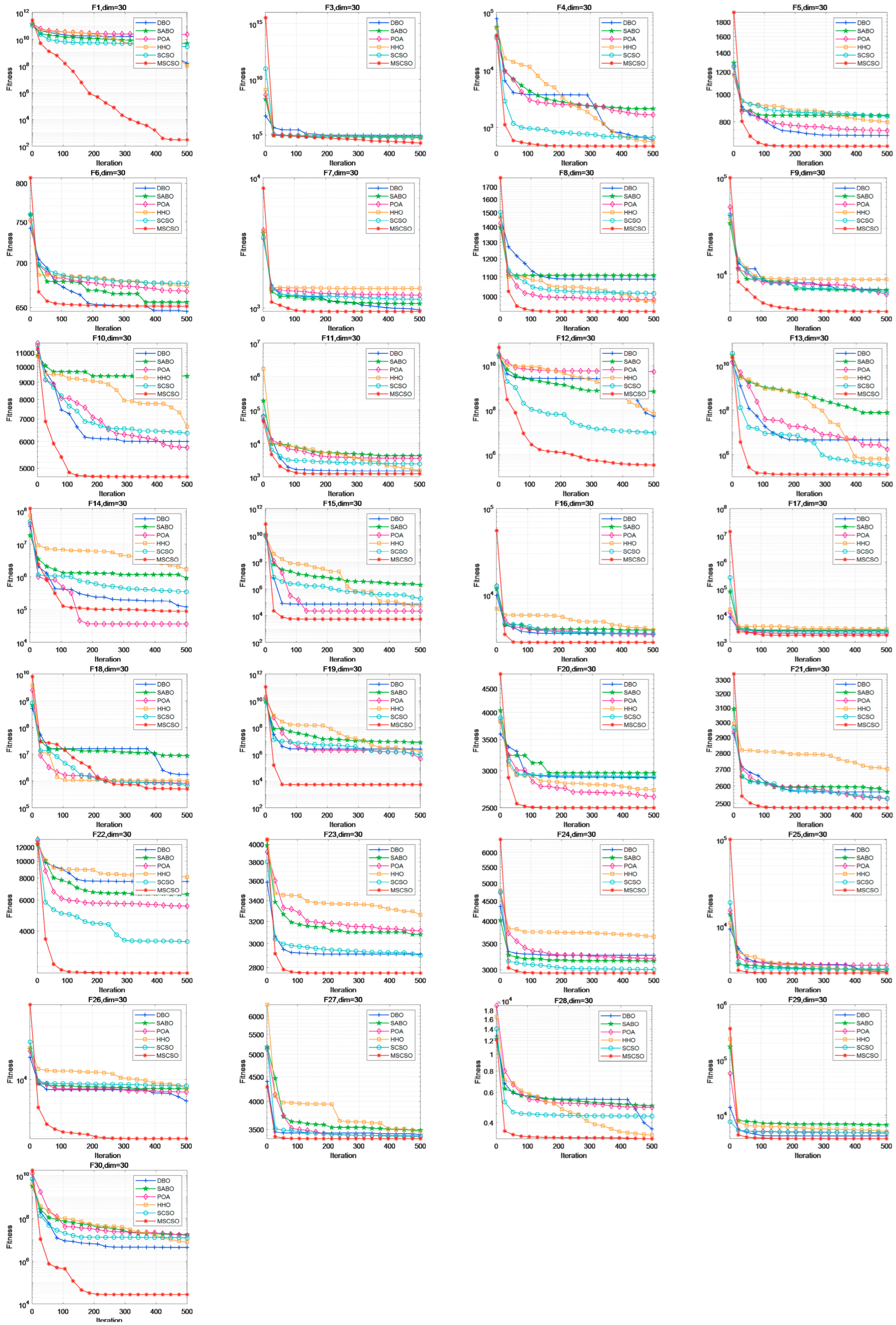
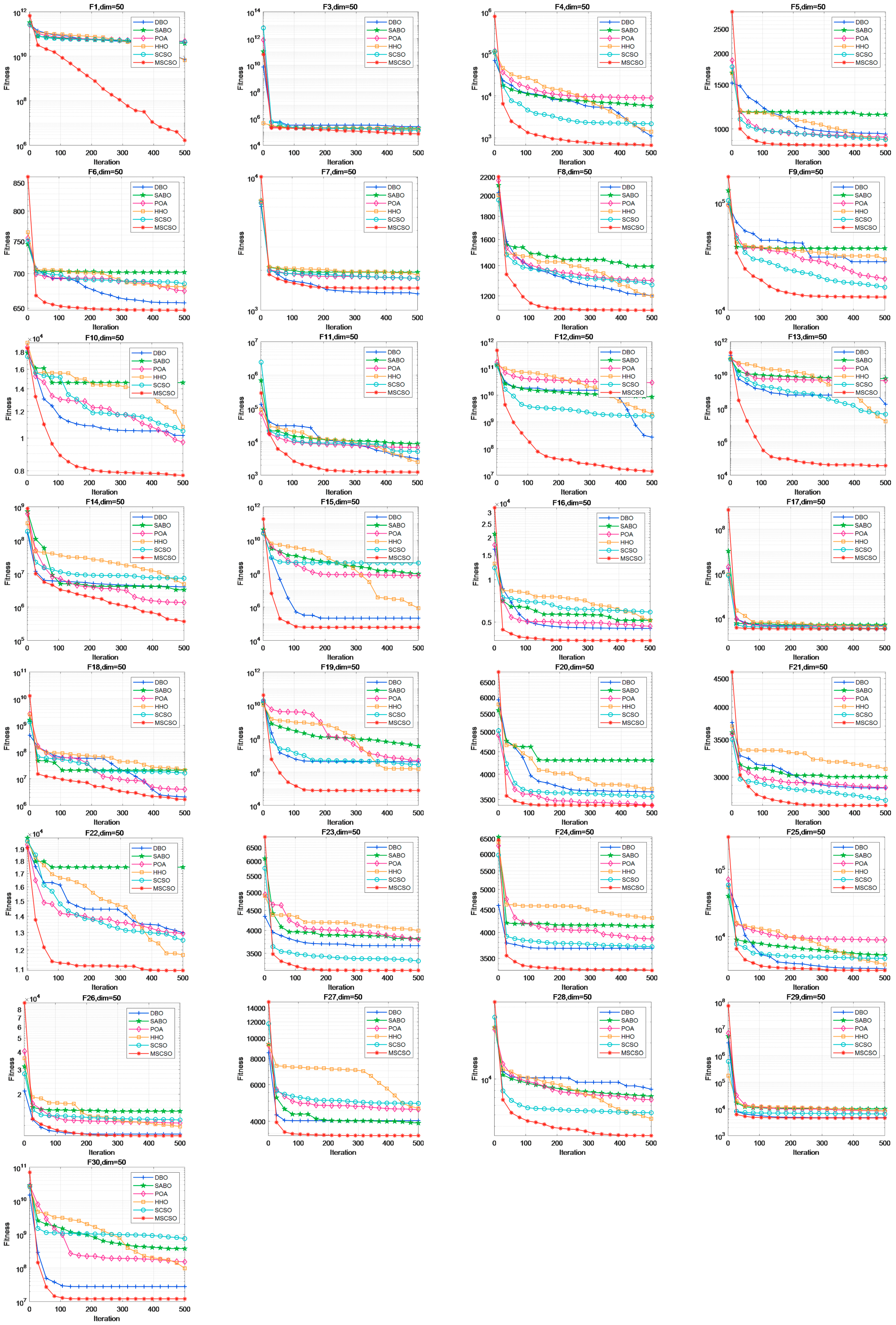
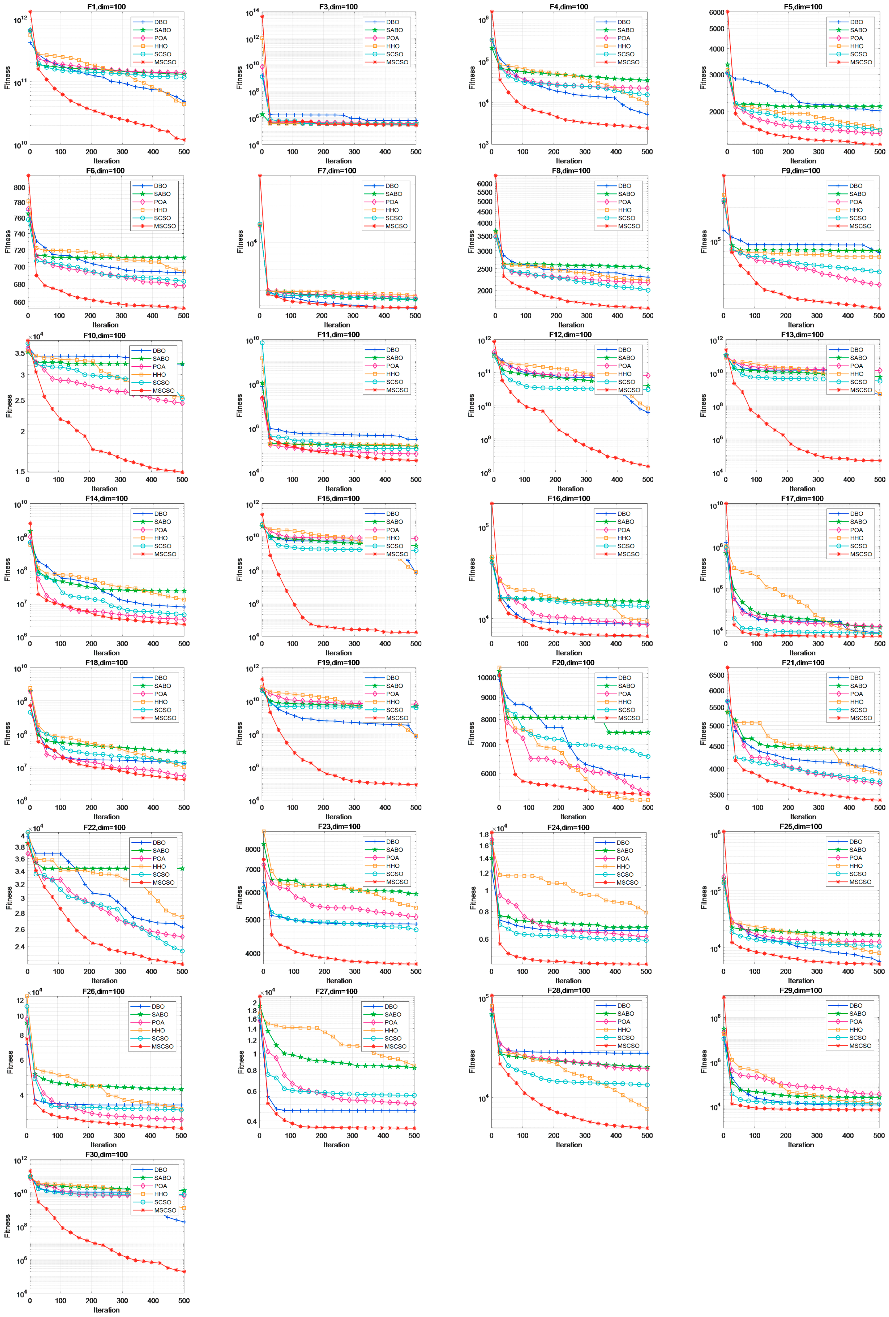
4.2.2. Convergence Plot Analysis Discussion
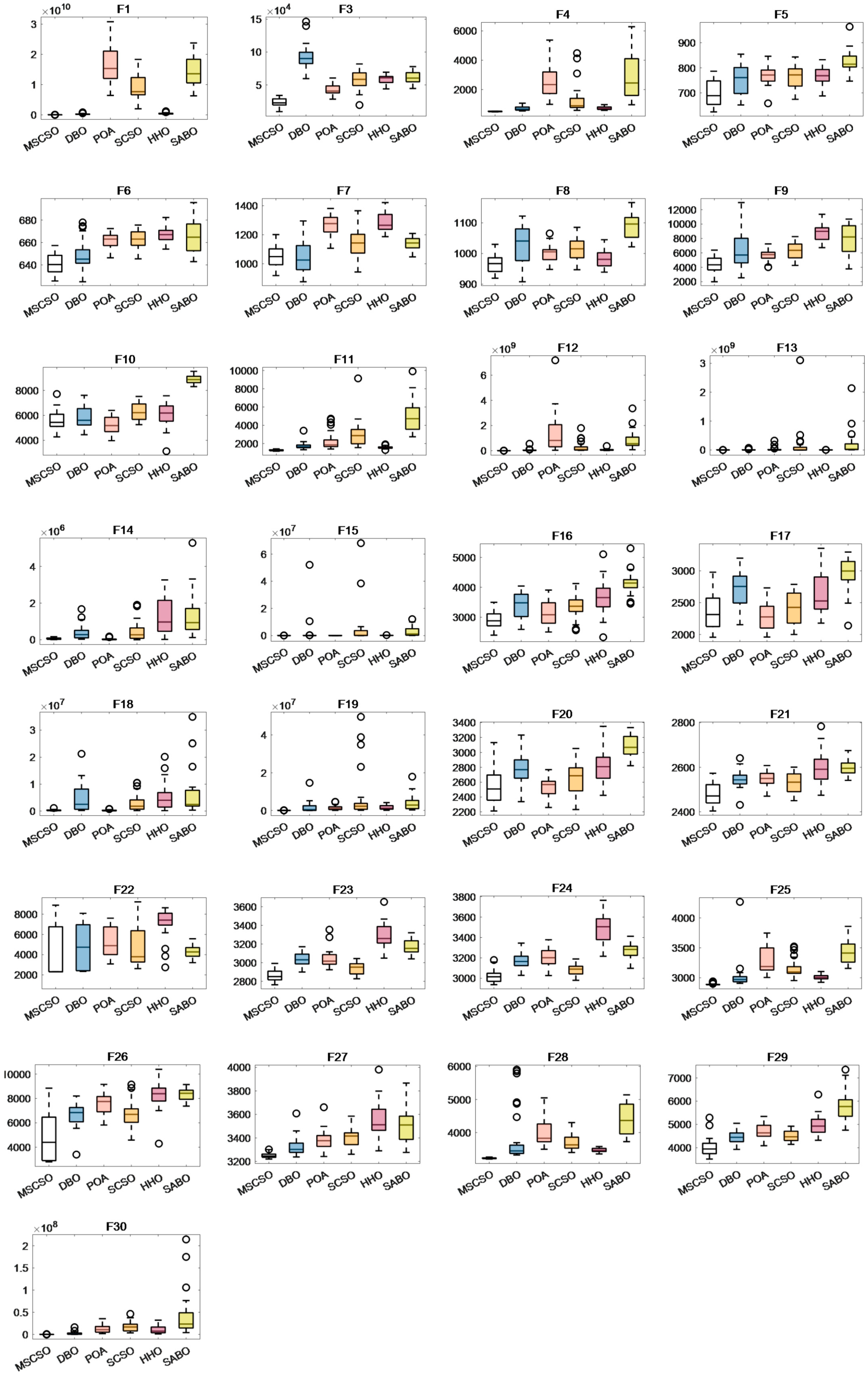
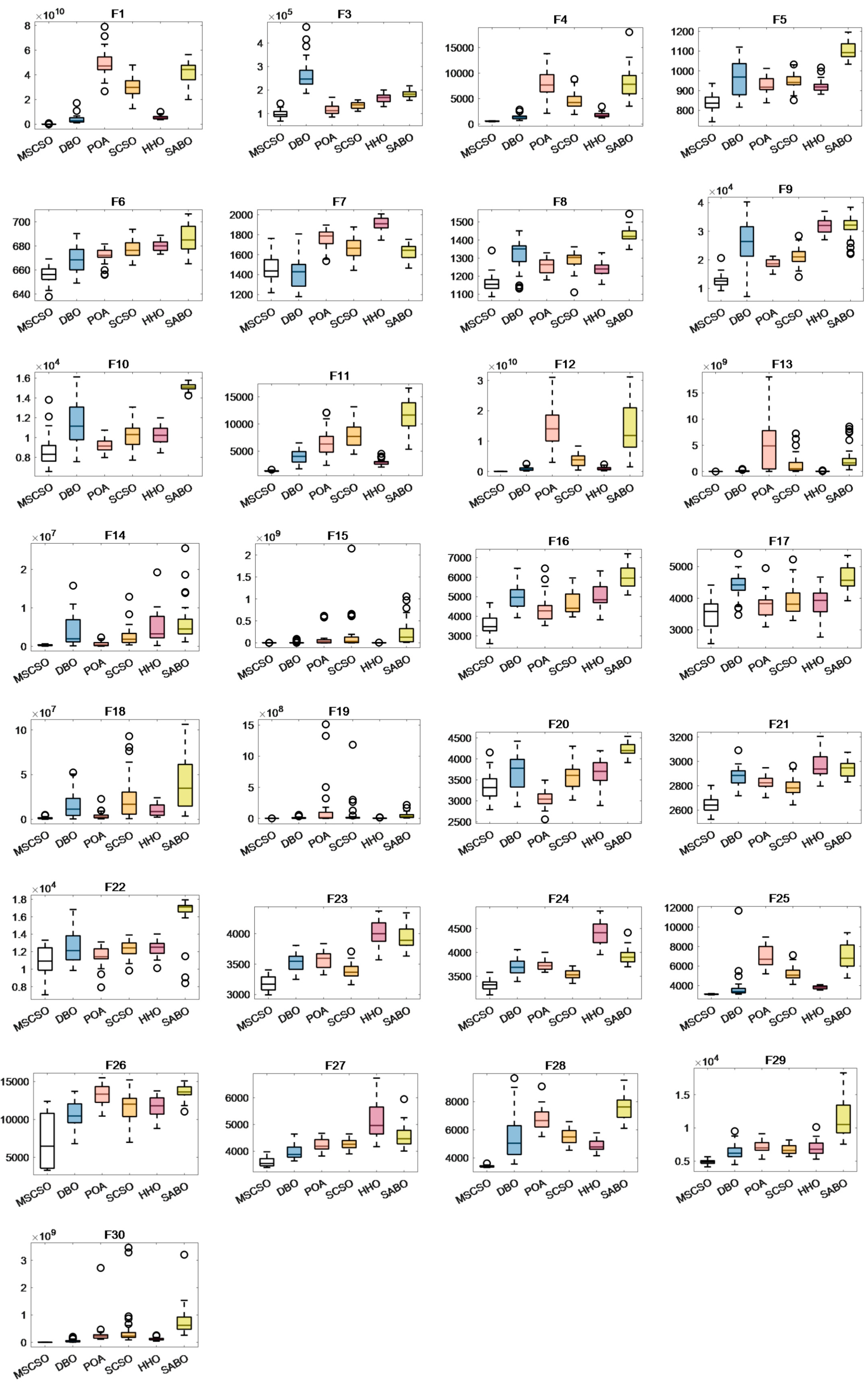
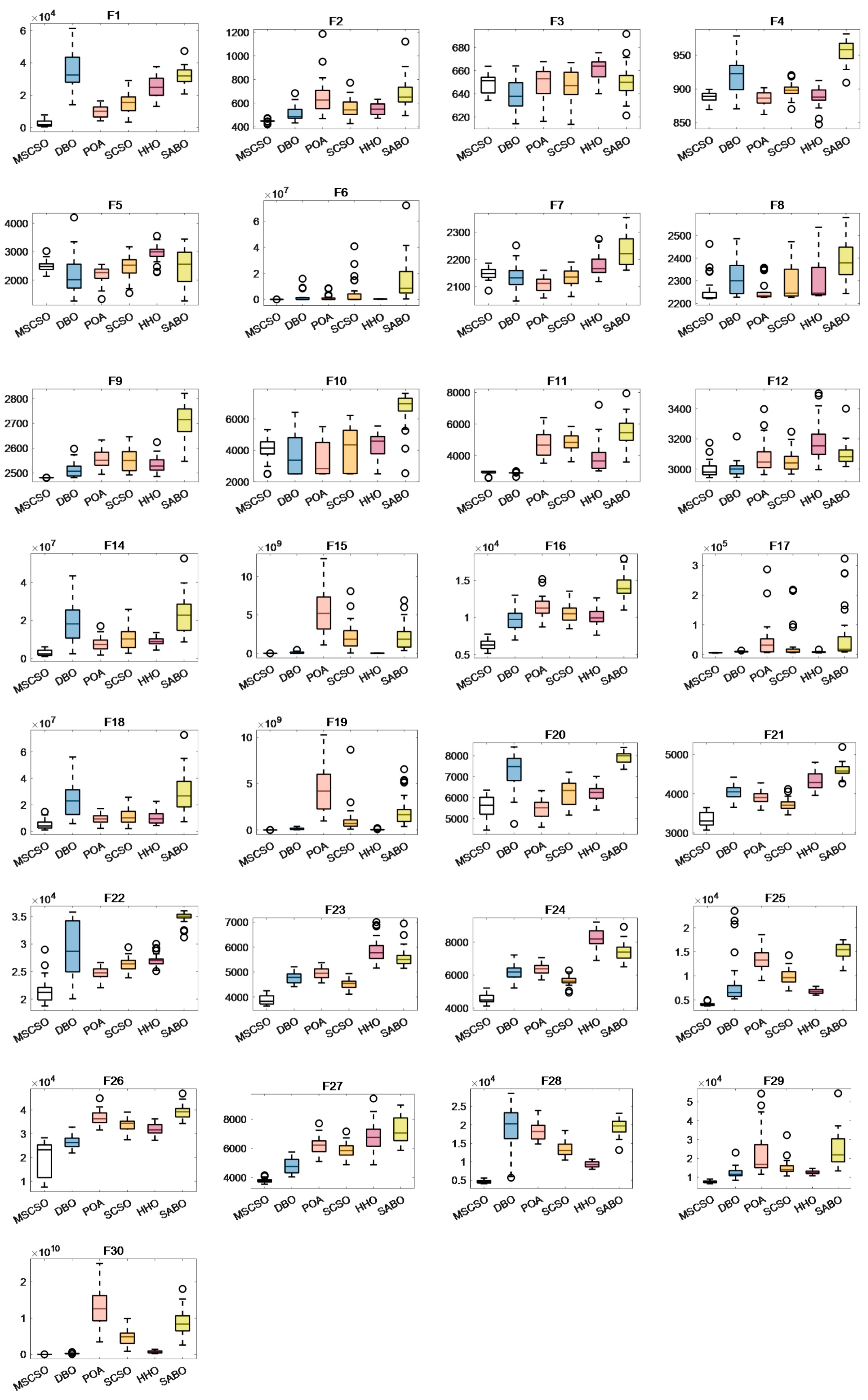
4.2.3. Boxplots Analysis
4.3. Non-Parametric Test
4.3.1. Wilcoxon Rank-Sum Test
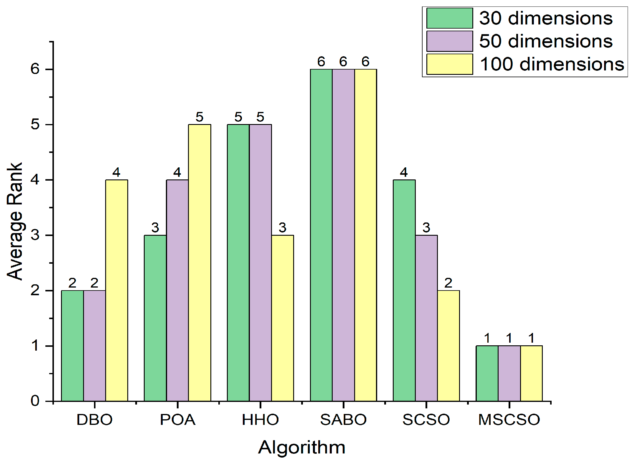
4.3.2. Friedman Test
5. Engineering Applications
5.1. Reducer Design Problems
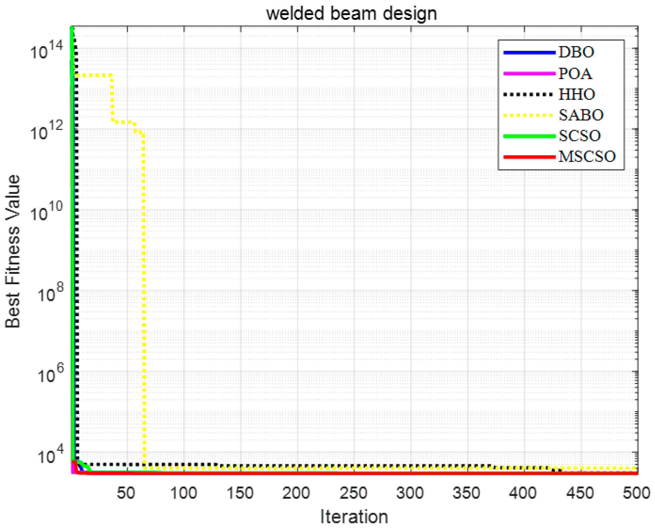
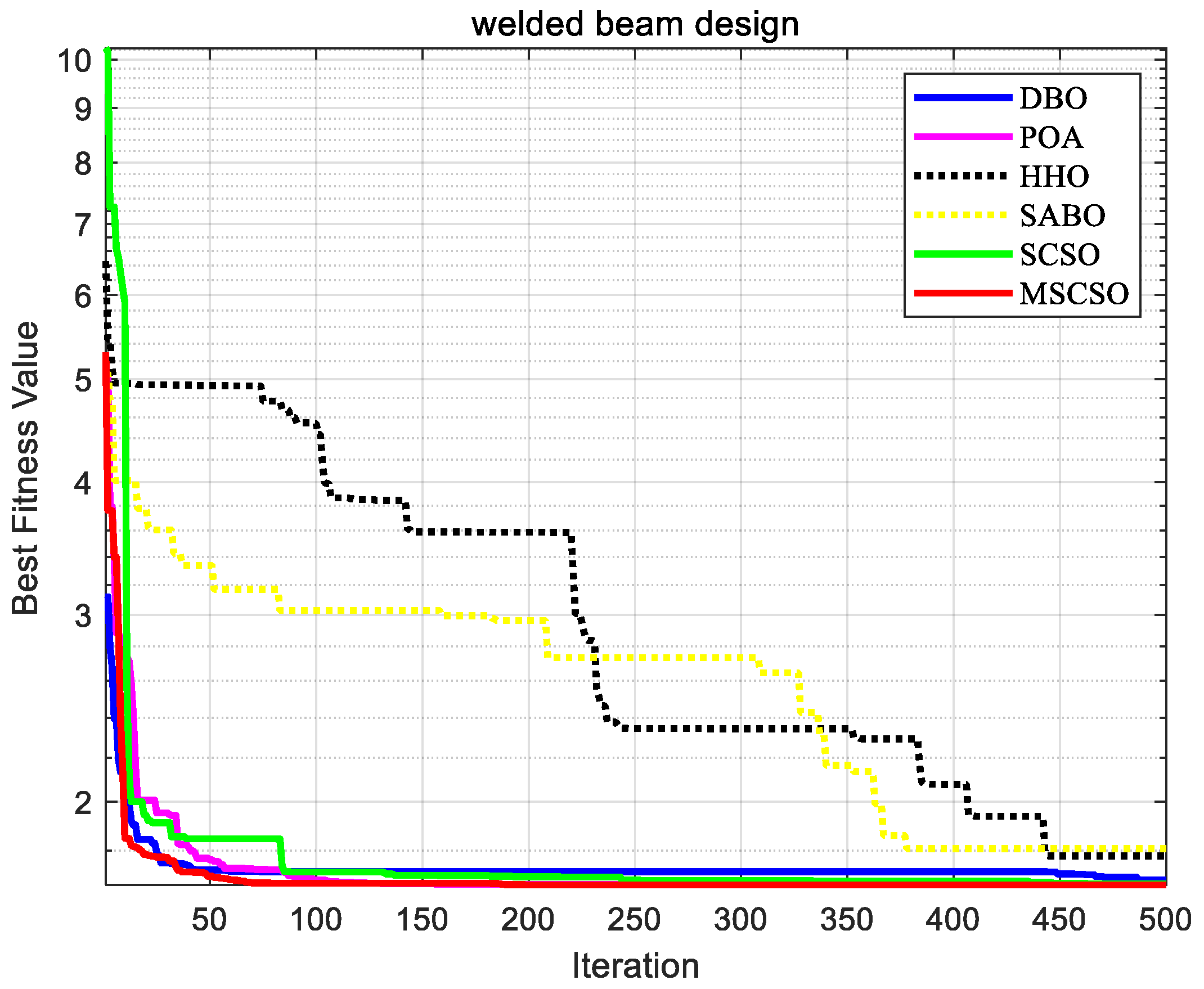
5.2. Welded Beam Design Problems
6. Conclusions
- Precision and convergence speed in unimodal functions: MSCSO demonstrated significantly higher precision and faster convergence speed in unimodal functions than other algorithms; it indicated MSCSO’s superiority in efficiently navigating and exploiting simple search landscapes.
- Robust optimization performance in hybrid and composition functions: MSCSO exhibited formidable optimization capabilities in hybrid and composition functions. It maintained a leading position in precision and convergence in most functions, underscoring its adaptability to diverse and complex optimization challenges. As the problem dimensionality increases, MSCSO’s performance became even more pronounced, demonstrating its prowess in tackling intricate and high-dimensional problems.
- Superiority confirmed by Wilcoxon rank-sum test: The Wilcoxon rank-sum test statistically validated that MSCSO outperforms other algorithms, providing robust evidence of its enhanced performance.
- Applicability in engineering problems: In practical engineering applications such as gearbox reducer and welded beam design problems, MSCSO produced solutions closer to the optimal solutions than five other algorithms. It highlighted MSCSO’s effectiveness in real-world scenarios and underscored its broad applicability in solving engineering optimization tasks.
Author Contributions
Funding
Data Availability Statement
Acknowledgments
Conflicts of Interest
Appendix A

| DBO | POA | HHO | SABO | SCSO | MSCSO | ||
|---|---|---|---|---|---|---|---|
| F1 | Mean | 3302398088 | 10390489898 | 1484653454 | 8799881201 | 8778375893 | 196284819 |
| Std | 3899252845 | 49823118066 | 5512734336 | 42119582938 | 30042244589 | 61728185.7 | |
| F3 | Mean | 66786.35118 | 22023.41482 | 18437.34617 | 16561.57008 | 13980.77039 | 17413.1313 |
| Std | 268106.3887 | 117684.1181 | 167032.023 | 182813.6126 | 133707.5058 | 99157.0174 | |
| F4 | Mean | 524.8249642 | 2726.350905 | 480.1093044 | 3027.911409 | 1656.421951 | 53.2610363 |
| Std | 1409.957618 | 7812.684022 | 1805.635567 | 8077.440603 | 4571.652584 | 567.295001 | |
| F5 | Mean | 84.95671361 | 40.22758238 | 31.12382383 | 43.52121811 | 36.853378 | 43.369063 |
| Std | 960.315895 | 926.2623231 | 922.5744492 | 1103.391257 | 948.8158352 | 838.558676 | |
| F6 | Mean | 11.32040522 | 6.237167532 | 4.065757496 | 12.3553266 | 7.190901281 | 7.57760074 |
| Std | 668.8507287 | 672.129517 | 679.9782754 | 686.2532994 | 677.4816775 | 656.270736 | |
| F7 | Mean | 135.3215707 | 90.41802472 | 69.8349611 | 79.64051781 | 110.3563116 | 131.381464 |
| Std | 1412.10116 | 1764.55676 | 1899.381916 | 1632.291613 | 1665.295017 | 1464.57607 | |
| F8 | Mean | 83.01299842 | 39.82495196 | 38.7444479 | 43.10136231 | 51.18661919 | 50.2141428 |
| Std | 1321.315603 | 1255.066828 | 1244.088564 | 1426.266704 | 1290.516019 | 1161.60697 | |
| F9 | Mean | 7710.747487 | 1529.036855 | 2603.718659 | 3922.344162 | 3210.250677 | 2219.92498 |
| Std | 25806.01922 | 18620.38525 | 32122.69238 | 31402.25016 | 21158.10829 | 12664.2894 | |
| F10 | Mean | 2272.307432 | 630.9933193 | 950.8373144 | 368.7032054 | 1119.804333 | 1573.49553 |
| Std | 11510.69442 | 9181.627844 | 10355.83564 | 15130.59108 | 10190.86836 | 8705.85798 | |
| F11 | Mean | 1322.890937 | 2470.236447 | 526.0597284 | 2745.167283 | 2255.918509 | 82.9280624 |
| Std | 4033.575553 | 6728.049967 | 2988.033843 | 11606.62784 | 7861.105679 | 1379.4339 | |
| F12 | Mean | 538853153.4 | 7237740245 | 567912624.7 | 7960953201 | 2208829317 | 6744695.91 |
| Std | 830186029.6 | 14648371591 | 954810132.7 | 13876884946 | 3833950125 | 10351644.2 | |
| F13 | Mean | 114150217.4 | 4494947129 | 41254837.95 | 2425906523 | 1903746602 | 35670.1713 |
| Std | 92502949.45 | 4707351617 | 33200051.09 | 2580833263 | 1474877114 | 56441.5596 | |
| F14 | Mean | 3974759.282 | 607675.3837 | 3910591.193 | 5374681.808 | 2703986.653 | 146418.047 |
| Std | 3918959.364 | 649914.5906 | 4748048.359 | 6304012.675 | 2681790.879 | 310747.588 | |
| F15 | Mean | 23480267.91 | 175874736.5 | 955411.5079 | 296542849.3 | 424171520.7 | 14866.0908 |
| Std | 9825049.542 | 88883732.08 | 1495111.31 | 238992978.7 | 189176839.5 | 28855.0623 | |
| F16 | Mean | 628.3633522 | 692.8244518 | 665.4755948 | 562.5161157 | 569.3277895 | 532.561722 |
| Std | 4989.421503 | 4372.086747 | 4990.462575 | 6001.400479 | 4672.412437 | 3592.24632 | |
| F17 | Mean | 429.73778 | 408.269056 | 485.9001181 | 365.0381958 | 479.430001 | 426.899651 |
| Std | 4413.380306 | 3774.015327 | 3828.298961 | 4618.758234 | 3919.009562 | 3492.97037 | |
| F18 | Mean | 14964943.25 | 4418438.238 | 6842181.004 | 28288404.34 | 24711295.34 | 1272072.92 |
| Std | 15796585.34 | 4262892.242 | 10795307.23 | 40890071.68 | 23837109.2 | 1564630.47 | |
| F19 | Mean | 13933122.64 | 362744484.7 | 3677685.849 | 50424696.53 | 222217039.8 | 14766.5931 |
| Std | 9116184.623 | 149962044.9 | 3069100.459 | 50048950.38 | 70718954.71 | 37005.8523 | |
| F20 | Mean | 410.2578286 | 213.5439526 | 308.4450941 | 168.3324002 | 294.2973357 | 345.601964 |
| Std | 3710.28514 | 3063.836687 | 3668.520885 | 4212.271348 | 3565.674877 | 3335.5459 | |
| F21 | Mean | 83.14094219 | 61.95986229 | 101.6349972 | 63.59623969 | 73.23544841 | 66.0088371 |
| Std | 2876.18541 | 2827.935196 | 2958.650285 | 2934.355452 | 2794.594213 | 2648.16974 | |
| F22 | Mean | 2015.922742 | 1074.838903 | 823.2283951 | 2343.895269 | 985.7160627 | 1602.4466 |
| Std | 12502.87764 | 11437.60931 | 12417.40035 | 16309.13028 | 12327.33491 | 10992.8653 | |
| F23 | Mean | 132.4932719 | 147.379751 | 206.4727144 | 180.1562827 | 123.2249366 | 114.317005 |
| Std | 3523.633457 | 3590.806985 | 3990.493109 | 3943.872193 | 3384.520633 | 3182.09634 | |
| F24 | Mean | 158.7447433 | 109.0159033 | 255.7003902 | 158.4743871 | 104.2052828 | 106.811743 |
| Std | 3695.170402 | 3733.672181 | 4419.94957 | 3913.251521 | 3537.007824 | 3320.05097 | |
| F25 | Mean | 1569.240404 | 1094.525409 | 162.705011 | 1287.475791 | 663.4378573 | 27.3972524 |
| Std | 3861.611951 | 6999.033404 | 3816.319194 | 7075.942069 | 5232.677992 | 3114.66829 | |
| F26 | Mean | 1118.232735 | 1865.600314 | 1342.11311 | 842.5372236 | 1614.13788 | 3234.80923 |
| Std | 11100.88082 | 12768.05974 | 11536.63164 | 13553.13631 | 11748.54079 | 5729.92126 | |
| F27 | Mean | 308.0431984 | 291.1735528 | 683.8444814 | 492.0369643 | 207.7881354 | 169.730378 |
| Std | 4010.032961 | 4339.722563 | 5155.284814 | 4642.827783 | 4274.549997 | 3611.67258 | |
| F28 | Mean | 2254.867558 | 755.4207857 | 441.8933227 | 825.6899025 | 570.2134973 | 87.1245666 |
| Std | 6131.061848 | 6815.875429 | 4758.024815 | 7617.282993 | 5661.331436 | 3377.80703 | |
| F29 | Mean | 1002.694976 | 621.4094541 | 1096.522217 | 1507.201481 | 822.3748579 | 485.91776 |
| Std | 6231.20715 | 7022.556572 | 7345.788008 | 9940.701573 | 6901.555629 | 4970.4202 | |
| F30 | Mean | 47489390.7 | 242380028.8 | 51564123.09 | 603825274.3 | 112349961.3 | 1336896.06 |
| Std | 60009001.81 | 346537086.2 | 128720404.5 | 734334649 | 220873074 | 2431763.66 |
| DBO | POA | HHO | SABO | SCSO | MSCSO | ||
|---|---|---|---|---|---|---|---|
| F1 | Mean | 64439785350 | 14679470611 | 7123064242 | 12786225157 | 13574141598 | 6191835519 |
| Std | 88946907692 | 1.44787 × 10¹¹ | 48058863472 | 1.56287 × 10¹¹ | 1.06645 × 10¹¹ | 1.8053 × 10¹⁰ | |
| F3 | Mean | 327312.9072 | 31671.50162 | 122549.3883 | 14531.95724 | 17342.92473 | 30730.8664 |
| Std | 730924.6607 | 305881.7838 | 372984.6991 | 348932.4274 | 320105.4844 | 298781.525 | |
| F4 | Mean | 15071.01887 | 6198.775365 | 1998.389853 | 6240.446945 | 4582.407811 | 1073.78027 |
| Std | 16471.56686 | 25602.81592 | 9838.835433 | 31928.30398 | 15787.59256 | 1733.29016 | |
| F5 | Mean | 255.9942286 | 64.41293008 | 46.42333274 | 113.6177764 | 60.19254203 | 50.4321657 |
| Std | 1737.151357 | 1606.074738 | 1673.752052 | 1930.352906 | 1632.976958 | 1371.77767 | |
| F6 | Mean | 13.17570887 | 3.748854711 | 3.847419004 | 5.791203439 | 4.652130833 | 3.18444647 |
| Std | 682.8830424 | 681.3642251 | 690.6116046 | 705.539359 | 686.9988035 | 664.088596 | |
| F7 | Mean | 230.5354516 | 80.11767378 | 131.0653554 | 183.3490029 | 204.1486638 | 207.995493 |
| Std | 2978.277946 | 3470.650798 | 3776.686954 | 3405.051846 | 3424.583953 | 2882.10396 | |
| F8 | Mean | 203.1690199 | 69.75688334 | 67.34965118 | 97.75941497 | 76.22128493 | 120.07328 |
| Std | 2215.08076 | 2086.033586 | 2132.86936 | 2360.188236 | 2085.977332 | 1762.19817 | |
| F9 | Mean | 6031.929811 | 3543.233864 | 4754.054793 | 4463.180529 | 5964.901628 | 1649.51376 |
| Std | 78882.20914 | 41704.00481 | 68787.89439 | 78575.29059 | 44974.51707 | 26104.6671 | |
| F10 | Mean | 5235.205338 | 1140.992805 | 1997.673166 | 731.0527176 | 1614.762398 | 2533.84918 |
| Std | 27335.04082 | 21101.19419 | 24224.20078 | 32359.4073 | 22747.04663 | 17293.8057 | |
| F11 | Mean | 68644.9515 | 18627.26318 | 38471.07732 | 42124.32695 | 23270.27405 | 6659.60843 |
| Std | 223448.5264 | 88617.44402 | 144597.4059 | 205655.4621 | 94315.73489 | 28493.7276 | |
| F12 | Mean | 2268580864 | 16365928649 | 2676065431 | 18164454902 | 13817550434 | 441613219 |
| Std | 7277633037 | 68930637601 | 11619528549 | 54872552598 | 36736964033 | 255071073 | |
| F13 | Mean | 192201584.9 | 5459325140 | 196797367.5 | 4378193430 | 3222776818 | 30025.803 |
| Std | 264566938.2 | 15150913501 | 340976541.6 | 8883083561 | 5668646842 | 65185.9529 | |
| F14 | Mean | 11153472.54 | 3516377.125 | 2237802.183 | 9886433.727 | 5827627.548 | 1513169.62 |
| Std | 18865348.02 | 7659394.616 | 9054348.956 | 23213173.86 | 10840847.18 | 2950801.58 | |
| F15 | Mean | 109477038 | 2800000225 | 10706452.68 | 1617740396 | 1859453612 | 24423.7711 |
| Std | 91000114.11 | 5414412363 | 18070615.52 | 2194201582 | 2129450783 | 44422.7137 | |
| F16 | Mean | 1437.527393 | 1401.778021 | 1127.143 | 1675.072261 | 1129.010461 | 687.019308 |
| Std | 9830.457777 | 11418.37002 | 10048.44809 | 14272.76565 | 10546.5916 | 6353.67028 | |
| F17 | Mean | 1446.023266 | 60266.75664 | 2015.379609 | 87948.15107 | 55169.84024 | 647.352039 |
| Std | 9522.423148 | 44338.51265 | 8111.732752 | 58510.76338 | 30618.69714 | 5891.41214 | |
| F18 | Mean | 13836695.43 | 3976344.651 | 4860168.729 | 14620039.89 | 5884800.631 | 3282615.36 |
| Std | 24279018.43 | 9314116.26 | 10333720.11 | 29683396.12 | 11376427.43 | 4933958.16 | |
| F19 | Mean | 104306523.7 | 2451264977 | 36239372.08 | 1655661585 | 1570265191 | 91064.6918 |
| Std | 139026655.4 | 4336804118 | 40238023.7 | 2111376240 | 1058246800 | 36491.2231 | |
| F20 | Mean | 873.1403828 | 485.1281919 | 391.7970499 | 288.1319208 | 574.8553324 | 492.113677 |
| Std | 7283.694865 | 5452.846214 | 6232.521204 | 7911.433915 | 6246.751869 | 5591.37673 | |
| F21 | Mean | 194.6733628 | 151.272736 | 240.8060467 | 174.772987 | 158.0561619 | 150.778371 |
| Std | 4034.475166 | 3900.882946 | 4336.474513 | 4609.40168 | 3732.258314 | 3344.92746 | |
| F22 | Mean | 4982.55286 | 1240.221994 | 1250.068268 | 1073.874386 | 1304.752149 | 2262.16708 |
| Std | 29603.2738 | 24731.09808 | 27107.14681 | 34789.05817 | 26263.40432 | 21557.4056 | |
| F23 | Mean | 228.9527889 | 228.6376536 | 463.797077 | 382.3292313 | 187.8860342 | 170.356698 |
| Std | 4774.38515 | 4964.923155 | 5861.948017 | 5563.140243 | 4534.221736 | 3861.13035 | |
| F24 | Mean | 434.7971439 | 293.7675921 | 601.9109496 | 544.0433336 | 292.4855238 | 254.89335 |
| Std | 6174.067484 | 6366.875405 | 8242.826952 | 7426.1978 | 5655.794757 | 4576.10926 | |
| F25 | Mean | 4971.625162 | 2146.970151 | 469.6290082 | 1718.771909 | 1580.137642 | 280.365032 |
| Std | 8528.152533 | 13375.00475 | 6799.205617 | 15072.28933 | 9867.156162 | 4069.11079 | |
| F26 | Mean | 2716.297116 | 2893.558169 | 2197.696998 | 2627.738246 | 2775.087158 | 7306.39958 |
| Std | 26555.3795 | 36793.64805 | 31943.81382 | 39199.66094 | 33818.41939 | 19838.3825 | |
| F27 | Mean | 517.8607132 | 624.4369159 | 1066.926374 | 907.8012227 | 519.8501265 | 142.25572 |
| Std | 4796.677845 | 6170.744599 | 6821.516679 | 7226.379513 | 5855.303843 | 3782.70941 | |
| F28 | Mean | 6867.524167 | 2361.314563 | 803.4499535 | 2055.769571 | 1887.503296 | 420.03276 |
| Std | 18557.442 | 18477.30251 | 9319.445458 | 19527.98794 | 13378.17802 | 4602.70205 | |
| F29 | Mean | 2818.558281 | 10708.19759 | 1042.989965 | 8864.106404 | 3914.703263 | 617.239425 |
| Std | 12278.1268 | 22161.34028 | 12642.23408 | 24025.07565 | 15093.16939 | 7535.46986 | |
| F30 | Mean | 109769797.4 | 4948234972 | 294385332.6 | 3570975523 | 2380766605 | 930694.966 |
| Std | 241833483.5 | 13085971393 | 669153209.3 | 8978885602 | 4603212747 | 981372.554 |
| DBO | POA | HHO | SABO | SCSO | |
|---|---|---|---|---|---|
| F1 | 3.6 × 10⁻¹¹ < 0.05 | 3.0 × 10⁻¹¹ < 0.05 | 3.0 × 10⁻¹¹ < 0.05 | 3.0 × 10⁻¹¹ < 0.05 | 3.0 × 10⁻¹¹ < 0.05 |
| F3 | 8.9 × 10⁻¹¹ < 0.05 | 3.2 × 10−01 > 0.05 | 1.1 × 10−05 < 0.05 | 2.8 × 10−06 < 0.05 | 3.2 × 10−02 < 0.05 |
| F4 | 3.0 × 10⁻¹¹ < 0.05 | 3.0 × 10⁻¹¹ < 0.05 | 3.0 × 10⁻¹¹ < 0.05 | 3.0 × 10⁻¹¹ < 0.05 | 3.0 × 10⁻¹¹ < 0.05 |
| F5 | 2.2 × 10−09 < 0.05 | 3.0 × 10⁻¹¹ < 0.05 | 3.0 × 10⁻¹¹ < 0.05 | 3.0 × 10⁻¹¹ < 0.05 | 3.0 × 10⁻¹¹ < 0.05 |
| F6 | 7.5 × 10−07 < 0.05 | 3.0 × 10⁻¹¹ < 0.05 | 3.0 × 10⁻¹¹ < 0.05 | 3.0 × 10⁻¹¹ < 0.05 | 3.0 × 10⁻¹¹ < 0.05 |
| F7 | 6.5 × 10−01 > 0.05 | 3.0 × 10⁻¹¹ < 0.05 | 3.0 × 10⁻¹¹ < 0.05 | 4.6 × 10⁻¹⁰ < 0.05 | 1.4 × 10−08 < 0.05 |
| F8 | 9.7 × 10⁻¹⁰ < 0.05 | 3.0 × 10⁻¹¹ < 0.05 | 3.0 × 10⁻¹¹ < 0.05 | 3.0 × 10⁻¹¹ < 0.05 | 3.0 × 10⁻¹¹ < 0.05 |
| F9 | 3.0 × 10⁻¹¹ < 0.05 | 3.0 × 10⁻¹¹ < 0.05 | 3.0 × 10⁻¹¹ < 0.05 | 3.0 × 10⁻¹¹ < 0.05 | 3.0 × 10⁻¹¹ < 0.05 |
| F10 | 7.3 × 10⁻¹⁰ < 0.05 | 5.1 × 10−07 < 0.05 | 4.0 × 10⁻¹¹ < 0.05 | 3.0 × 10⁻¹¹ < 0.05 | 1.5 × 10−09 < 0.05 |
| F11 | 3.0 × 10⁻¹¹ < 0.05 | 3.0 × 10⁻¹¹ < 0.05 | 3.0 × 10⁻¹¹ < 0.05 | 3.0 × 10⁻¹¹ < 0.05 | 3.0 × 10⁻¹¹ < 0.05 |
| F12 | 2.3 × 10⁻¹⁰ < 0.05 | 3.0 × 10⁻¹¹ < 0.05 | 6.0 × 10⁻¹¹ < 0.05 | 3.0 × 10⁻¹¹ < 0.05 | 3.0 × 10⁻¹¹ < 0.05 |
| F13 | 3.0 × 10⁻¹¹ < 0.05 | 3.0 × 10⁻¹¹ < 0.05 | 3.0 × 10⁻¹¹ < 0.05 | 3.0 × 10⁻¹¹ < 0.05 | 3.0 × 10⁻¹¹ < 0.05 |
| F14 | 4.6 × 10−08 < 0.05 | 1.6 × 10−05 < 0.05 | 1.1 × 10−09 < 0.05 | 3.0 × 10⁻¹¹ < 0.05 | 7.3 × 10⁻¹⁰ < 0.05 |
| F15 | 3.0 × 10⁻¹¹ < 0.05 | 3.0 × 10⁻¹¹ < 0.05 | 3.0 × 10⁻¹¹ < 0.05 | 3.0 × 10⁻¹¹ < 0.05 | 3.0 × 10⁻¹¹ < 0.05 |
| F16 | 8.9 × 10⁻¹¹ < 0.05 | 3.3 × 10⁻¹¹ < 0.05 | 3.0 × 10⁻¹¹ < 0.05 | 3.0 × 10⁻¹¹ < 0.05 | 3.0 × 10⁻¹¹ < 0.05 |
| F17 | 3.0 × 10⁻¹¹ < 0.05 | 3.0 × 10⁻¹¹ < 0.05 | 3.3 × 10⁻¹¹ < 0.05 | 3.0 × 10⁻¹¹ < 0.05 | 1.2 × 10⁻¹⁰ < 0.05 |
| F18 | 1.8 × 10−09 < 0.05 | 1.8 × 10−06 < 0.05 | 7.5 × 10−07 < 0.05 | 3.0 × 10⁻¹¹ < 0.05 | 1.4 × 10−07 < 0.05 |
| F19 | 3.0 × 10⁻¹¹ < 0.05 | 3.0 × 10⁻¹¹ < 0.05 | 3.0 × 10⁻¹¹ < 0.05 | 3.0 × 10⁻¹¹ < 0.05 | 3.0 × 10⁻¹¹ < 0.05 |
| F20 | 7.7 × 10−09 < 0.05 | 3.4 × 10−01 > 0.05 | 5.3 × 10−03 < 0.05 | 3.0 × 10⁻¹¹ < 0.05 | 5.5 × 10−03 < 0.05 |
| F21 | 4.5 × 10⁻¹¹ < 0.05 | 3.0 × 10⁻¹¹ < 0.05 | 3.0 × 10⁻¹¹ < 0.05 | 3.0 × 10⁻¹¹ < 0.05 | 1.6 × 10⁻¹⁰ < 0.05 |
| F22 | 2.0 × 10−08 < 0.05 | 5.1 × 10−07 < 0.05 | 1.7 × 10⁻¹⁰ < 0.05 | 3.0 × 10⁻¹¹ < 0.05 | 4.6 × 10−08 < 0.05 |
| F23 | 3.0 × 10⁻¹¹ < 0.05 | 3.0 × 10⁻¹¹ < 0.05 | 3.0 × 10⁻¹¹ < 0.05 | 3.0 × 10⁻¹¹ < 0.05 | 1.2 × 10⁻¹⁰ < 0.05 |
| F24 | 3.0 × 10⁻¹¹ < 0.05 | 3.0 × 10⁻¹¹ < 0.05 | 3.0 × 10⁻¹¹ < 0.05 | 3.0 × 10⁻¹¹ < 0.05 | 4.5 × 10⁻¹¹ < 0.05 |
| F25 | 3.0 × 10⁻¹¹ < 0.05 | 3.0 × 10⁻¹¹ < 0.05 | 3.0 × 10⁻¹¹ < 0.05 | 3.0 × 10⁻¹¹ < 0.05 | 3.0 × 10⁻¹¹ < 0.05 |
| F26 | 6.9 × 10−03 < 0.05 | 3.0 × 10⁻¹¹ < 0.05 | 3.6 × 10⁻¹¹ < 0.05 | 3.0 × 10⁻¹¹ < 0.05 | 1.4 × 10⁻¹⁰ < 0.05 |
| F27 | 1.9 × 10⁻¹⁰ < 0.05 | 3.0 × 10⁻¹¹ < 0.05 | 3.0 × 10⁻¹¹ < 0.05 | 3.0 × 10⁻¹¹ < 0.05 | 3.0 × 10⁻¹¹ < 0.05 |
| F28 | 3.0 × 10⁻¹¹ < 0.05 | 3.0 × 10⁻¹¹ < 0.05 | 3.0 × 10⁻¹¹ < 0.05 | 3.0 × 10⁻¹¹ < 0.05 | 3.0 × 10⁻¹¹ < 0.05 |
| F29 | 3.6 × 10⁻¹¹ < 0.05 | 3.0 × 10⁻¹¹ < 0.05 | 3.0 × 10⁻¹¹ < 0.05 | 3.0 × 10⁻¹¹ < 0.05 | 3.0 × 10⁻¹¹ < 0.05 |
| F30 | 3.0 × 10⁻¹¹ < 0.05 | 3.0 × 10⁻¹¹ < 0.05 | 3.0 × 10⁻¹¹ < 0.05 | 3.0 × 10⁻¹¹ < 0.05 | 3.0 × 10⁻¹¹ < 0.05 |
| DBO | POA | HHO | SABO | SCSO | |
|---|---|---|---|---|---|
| F1 | 1.8 × 10−09 < 0.05 | 1.8 × 10−06 < 0.05 | 7.5 × 10−07 < 0.05 | 3.0 × 10⁻¹¹ < 0.05 | 1.4 × 10−07 < 0.05 |
| F3 | 8.9 × 10⁻¹¹ < 0.05 | 4.9 × 10−01 > 0.05 | 1.1 × 10−05 < 0.05 | 2.8 × 10−06 < 0.05 | 3.2 × 10−02 < 0.05 |
| F4 | 3.0 × 10⁻¹¹ < 0.05 | 3.0 × 10⁻¹¹ < 0.05 | 3.0 × 10⁻¹¹ < 0.05 | 3.0 × 10⁻¹¹ < 0.05 | 3.0 × 10⁻¹¹ < 0.05 |
| F5 | 2.2 × 10−09 < 0.05 | 3.0 × 10⁻¹¹ < 0.05 | 3.0 × 10⁻¹¹ < 0.05 | 3.0 × 10⁻¹¹ < 0.05 | 3.0 × 10⁻¹¹ < 0.05 |
| F6 | 7.5 × 10−07 < 0.05 | 3.0 × 10⁻¹¹ < 0.05 | 3.0 × 10⁻¹¹ < 0.05 | 3.0 × 10⁻¹¹ < 0.05 | 3.0 × 10⁻¹¹ < 0.05 |
| F7 | 7.5 × 10−07 < 0.05 | 3.0 × 10⁻¹¹ < 0.05 | 3.0 × 10⁻¹¹ < 0.05 | 4.6 × 10⁻¹⁰ < 0.05 | 1.4 × 10−08 < 0.05 |
| F8 | 9.7 × 10⁻¹⁰ < 0.05 | 3.0 × 10⁻¹¹ < 0.05 | 3.0 × 10⁻¹¹ < 0.05 | 3.0 × 10⁻¹¹ < 0.05 | 3.0 × 10⁻¹¹ < 0.05 |
| F9 | 3.0 × 10⁻¹¹ < 0.05 | 3.0 × 10⁻¹¹ < 0.05 | 3.0 × 10⁻¹¹ < 0.05 | 3.0 × 10⁻¹¹ < 0.05 | 3.0 × 10⁻¹¹ < 0.05 |
| F10 | 7.3 × 10⁻¹⁰ < 0.05 | 5.1 × 10−07 < 0.05 | 3.0 × 10⁻¹¹ < 0.05 | 3.0 × 10⁻¹¹ < 0.05 | 1.5 × 10−09 < 0.05 |
| F11 | 3.0 × 10⁻¹¹ < 0.05 | 3.0 × 10⁻¹¹ < 0.05 | 3.0 × 10⁻¹¹ < 0.05 | 3.0 × 10⁻¹¹ < 0.05 | 3.0 × 10⁻¹¹ < 0.05 |
| F12 | 3.0 × 10⁻¹¹ < 0.05 | 3.0 × 10⁻¹¹ < 0.05 | 3.0 × 10⁻¹¹ < 0.05 | 3.0 × 10⁻¹¹ < 0.05 | 3.0 × 10⁻¹¹ < 0.05 |
| F13 | 2.3 × 10⁻¹⁰ < 0.05 | 3.0 × 10⁻¹¹ < 0.05 | 3.0 × 10⁻¹¹ < 0.05 | 3.0 × 10⁻¹¹ < 0.05 | 3.0 × 10⁻¹¹ < 0.05 |
| F14 | 3.0 × 10⁻¹¹ < 0.05 | 3.0 × 10⁻¹¹ < 0.05 | 3.0 × 10⁻¹¹ < 0.05 | 3.0 × 10⁻¹¹ < 0.05 | 3.0 × 10⁻¹¹ < 0.05 |
| F15 | 3.0 × 10⁻¹¹ < 0.05 | 3.0 × 10⁻¹¹ < 0.05 | 3.0 × 10⁻¹¹ < 0.05 | 3.0 × 10⁻¹¹ < 0.05 | 3.0 × 10⁻¹¹ < 0.05 |
| F16 | 8.9 × 10⁻¹¹ < 0.05 | 3.3 × 10⁻¹¹ < 0.05 | 3.0 × 10⁻¹¹ < 0.05 | 3.0 × 10⁻¹¹ < 0.05 | 3.0 × 10⁻¹¹ < 0.05 |
| F17 | 3.0 × 10⁻¹¹ < 0.05 | 3.0 × 10⁻¹¹ < 0.05 | 3.0 × 10⁻¹¹ < 0.05 | 3.0 × 10⁻¹¹ < 0.05 | 1.2 × 10⁻¹⁰ < 0.05 |
| F18 | 1.8 × 10−09 < 0.05 | 1.8 × 10−06 < 0.05 | 7.5 × 10−07 < 0.05 | 3.0 × 10⁻¹¹ < 0.05 | 1.4 × 10−07 < 0.05 |
| F19 | 3.0 × 10⁻¹¹ < 0.05 | 3.0 × 10⁻¹¹ < 0.05 | 3.0 × 10⁻¹¹ < 0.05 | 3.0 × 10⁻¹¹ < 0.05 | 3.0 × 10⁻¹¹ < 0.05 |
| F20 | 7.7 × 10−09 < 0.05 | 2.3 × 10−01 > 0.05 | 5.3 × 10−03 < 0.05 | 3.0 × 10⁻¹¹ < 0.05 | 5.5 × 10−03 < 0.05 |
| F21 | 4.5 × 10⁻¹¹ < 0.05 | 3.0 × 10⁻¹¹ < 0.05 | 3.0 × 10⁻¹¹ < 0.05 | 3.0 × 10⁻¹¹ < 0.05 | 1.6 × 10⁻¹⁰ < 0.05 |
| F22 | 2.0 × 10−08 < 0.05 | 5.1 × 10−07 < 0.05 | 3.0 × 10⁻¹¹ < 0.05 | 3.0 × 10⁻¹¹ < 0.05 | 4.6 × 10−08 < 0.05 |
| F23 | 3.0 × 10⁻¹¹ < 0.05 | 3.0 × 10⁻¹¹ < 0.05 | 3.0 × 10⁻¹¹ < 0.05 | 3.0 × 10⁻¹¹ < 0.05 | 1.2 × 10⁻¹⁰ < 0.05 |
| F24 | 3.0 × 10⁻¹¹ < 0.05 | 3.0 × 10⁻¹¹ < 0.05 | 3.0 × 10⁻¹¹ < 0.05 | 3.0 × 10⁻¹¹ < 0.05 | 3.0 × 10⁻¹¹ < 0.05 |
| F25 | 3.0 × 10⁻¹¹ < 0.05 | 3.0 × 10⁻¹¹ < 0.05 | 3.0 × 10⁻¹¹ < 0.05 | 3.0 × 10⁻¹¹ < 0.05 | 3.0 × 10⁻¹¹ < 0.05 |
| F26 | 6.9 × 10−03 < 0.05 | 3.0 × 10⁻¹¹ < 0.05 | 3.0 × 10⁻¹¹ < 0.05 | 3.0 × 10⁻¹¹ < 0.05 | 1.4 × 10⁻¹⁰ < 0.05 |
| F27 | 1.9 × 10⁻¹⁰ < 0.05 | 3.0 × 10⁻¹¹ < 0.05 | 3.0 × 10⁻¹¹ < 0.05 | 3.0 × 10⁻¹¹ < 0.05 | 3.0 × 10⁻¹¹ < 0.05 |
| F28 | 3.0 × 10⁻¹¹ < 0.05 | 3.0 × 10⁻¹¹ < 0.05 | 3.0 × 10⁻¹¹ < 0.05 | 3.0 × 10⁻¹¹ < 0.05 | 3.0 × 10⁻¹¹ < 0.05 |
| F29 | 7.6 × 10−05 < 0.05 | 1.3 × 10−07 < 0.05 | 5.4 × 10−09 < 0.05 | 3.0 × 10⁻¹¹ < 0.05 | 1.7 × 10−07 < 0.05 |
| F30 | 3.0 × 10⁻¹¹ < 0.05 | 3.0 × 10⁻¹¹ < 0.05 | 3.0 × 10⁻¹¹ < 0.05 | 3.0 × 10⁻¹¹ < 0.05 | 3.0 × 10⁻¹¹ < 0.05 |
References
- Rezk, H.; Olabi, A.G.; Wilberforce, T.; Sayed, E.T. Metaheuristic optimization algorithms for real-world electrical and civil engineering application: A Review. Results Eng. 2024, 23, 102437. [Google Scholar] [CrossRef]
- Jia, H. Design of fruit fly optimization algorithm based on Gaussian distribution and its application to image processing. Syst. Soft Comput. 2024, 6, 200090. [Google Scholar] [CrossRef]
- Aishwaryaprajna; Kirubarajan, T.; Tharmarasa, R.; Rowe, J.E. UAV path planning in presence of occlusions as noisy combinatorial multi-objective optimisation. Int. J. Bio-Inspired Comput. 2023, 21, 209–217. [Google Scholar] [CrossRef]
- Wang, K.; Guo, M.; Dai, C.; Li, Z.; Wu, C.; Li, J. An effective metaheuristic technology of people duality psychological tendency and feedback mechanism-based Inherited Optimization Algorithm for solving engineering applications. Expert Syst. Appl. 2024, 244, 122732. [Google Scholar] [CrossRef]
- Lan, F.; Castellani, M.; Zheng, S.; Wang, Y. The SVD-enhanced bee algorithm, a novel procedure for point cloud registration. Swarm Evol. Comput. 2024, 88, 101590. [Google Scholar] [CrossRef]
- Zhou, S.; Shi, Y.; Wang, D.; Xu, X.; Xu, M.; Deng, Y. Election Optimizer Algorithm: A New Meta-Heuristic Optimization Algorithm for Solving Industrial Engineering Design Problems. Mathematics 2024, 12, 1513. [Google Scholar] [CrossRef]
- Kennedy, J.; Eberhart, R. Particle swarm optimization. In Proceedings of the International Conference on Neural Networks 1995, Perth, WA, Australia, 27 November–1 December 1995; pp. 1942–1948. [Google Scholar]
- Dorigo, M. Positive Feedback as a Search Strategy; Technical Report; Dipartimento di Elettronica, Politecnico di Milano: Milan, Italy, 1991; pp. 16–91. [Google Scholar]
- Holland, J. Genetic algorithms. Sci. Am. 1992, 267, 66–72. [Google Scholar] [CrossRef]
- Xue, J.; Shen, B. A novel swarm intelligence optimization approach: Sparrow search algorithm. Syst. Sci. Control. Eng. 2020, 8, 22–34. [Google Scholar] [CrossRef]
- Xue, J.; Shen, B. Dung beetle optimizer: A new meta-heuristic algorithm for global optimization. J. Supercomput. 2023, 79, 7305–7336. [Google Scholar] [CrossRef]
- Trojovský, P.; Dehghani, M. Pelican optimization algorithm: A novel nature-inspired algorithm for engineering applications. Sensors 2022, 22, 855. [Google Scholar] [CrossRef]
- Heidari, A.A.; Mirjalili, S.; Faris, H.; Aljarah, I.; Mafarja, M.; Chen, H. Harris Hawks optimization: Algorithm and applications. Future Gener. Comput. Syst. 2019, 97, 849–872. [Google Scholar] [CrossRef]
- Trojovský, P.; Dehghani, M. Subtraction-average-based optimizer: A new swarm-inspired metaheuristic algorithm for solving optimization problems. Biomimetics 2023, 8, 149. [Google Scholar] [CrossRef] [PubMed]
- Seyyedabbasi, A.; Kiani, F. Sand Cat swarm optimization: A nature-inspired algorithm to solve global optimization problems Figure 3. Eng. Comput. 2023, 39, 2627–2651. [Google Scholar] [CrossRef]
- Qiu, Y.; Zhou, J. Short-term rockburst damage assessment in burst-prone mines: An explainable XGBOOST hybrid model with SCSO algorithm. Rock Mech. Rock Eng. 2023, 56, 8745–8770. [Google Scholar] [CrossRef]
- Aghaei, V.T.; SeyyedAbbasi, A.; Rasheed, J.; Abu-Mahfouz, A.M. Sand cat swarm optimization-based feedback controller design for nonlinear systems. Heliyon 2023, 9, e13885. [Google Scholar] [CrossRef] [PubMed]
- Adegboye, O.R.; Feda, A.K.; Ojekemi, O.R.; Agyekum, E.B.; Khan, B.; Kamel, S. DGS-SCSO: Enhancing Sand Cat Swarm Optimization with Dynamic Pinhole Imaging and Golden Sine Algorithm for improved numerical optimization performance. Sci. Rep. 2024, 14, 1491. [Google Scholar] [CrossRef] [PubMed]
- Niu, Y.; Yan, X.; Wang, Y.; Niu, Y. An improved sand cat swarm optimization for moving target search by UAV. Expert Syst. Appl. 2024, 238, 122189. [Google Scholar] [CrossRef]
- Seyyedabbasi, A. A reinforcement learning-based metaheuristic algorithm for solving global optimization problems. Adv. Eng. Softw. 2023, 178, 103411. [Google Scholar] [CrossRef]
- Kiani, F.; Nematzadeh, S.; Anka, F.A.; Findikli, M.A. Chaotic sand cat swarm optimization. Mathematics 2023, 11, 2340. [Google Scholar] [CrossRef]
- Kiani, F.; Anka, F.A.; Erenel, F. PSCSO: Enhanced sand cat swarm optimization inspired by the political system to solve complex problems. Adv. Eng. Softw. 2023, 178, 103423. [Google Scholar] [CrossRef]
- Wolpert, D.H.; Macready, W.G. No free lunch theorems for optimization. IEEE Trans. Evol. Comput. 1997, 1, 67–82. [Google Scholar] [CrossRef]
- Luogeng, H. Applications of Number Theory to Modern Analysis; Science Press: Beijing, China, 1978. [Google Scholar]
- Zhu, F.; Li, G.; Tang, H.; Li, Y.; Lv, X.; Wang, X. Dung beetle optimization algorithm based on quantum computing and multi-strategy fusion for solving engineering problems. Expert Syst. Appl. 2024, 236, 121219. [Google Scholar] [CrossRef]
- Qiu, Y.; Yang, X.; Chen, S. An improved gray wolf optimization algorithm solving to functional optimization and engineering design problems. Sci. Rep. 2024, 14, 14190. [Google Scholar] [CrossRef] [PubMed]
- Gao, P.; Ding, H.; Xu, R. Whale optimization algorithm based on skew tent chaotic map and nonlinear strategy. Acad. J. Comput. Inf. Sci. 2021, 4, 91–97. [Google Scholar] [CrossRef]
- Li, Q.; Shi, H.; Zhao, W.; Ma, C. Enhanced Dung Beetle Optimization Algorithm for Practical Engineering Optimization. Mathematics 2024, 12, 1084. [Google Scholar] [CrossRef]
- Derrac, J.; García, S.; Molina, D.; Herrera, F. A practical tutorial on the use of nonparametric statistical tests as a methodology for comparing evolutionary and swarm intelligence algorithms. Swarm Evol. Comput. 2021, 1, 3–18. [Google Scholar] [CrossRef]
- Bayzidi, H.; Talatahari, S.; Saraee, M.; Lamarche, C.P. Social network search for solving engineering optimization prob lems. Comput. Intell. Neurosci. 2021, 2021, 8548639. [Google Scholar] [CrossRef]


| Improved SCSO | Research Gap |
|---|---|
| DGS-SCSO [18] | Time consumption is long |
| ISCSO [19] | Unable to apply multi-objective coordinated search |
| RLSCSO [20] | There exists premature convergence on specific problems |
| CSCSO [21] | Not suitable for multi-objective and multi-dimensional problems |
| Algorithm | Basic Parameters |
|---|---|
| DBO | P-Percent = 0.2 |
| POA | I = round (1 + rand (1, 1)) |
| HHO | E0 ∈ [−1, 1], E1 ∈ [0, 2] |
| SABO | I = round (1 + rand + rand) |
| SCSO | SM = 2, P = [1, 360] |
| MSCSO | SM = 2, P = [1, 360] |
| DBO | POA | HHO | SABO | SCSO | MSCSO | ||
|---|---|---|---|---|---|---|---|
| F1 | Mean | 181061557.9 | 5660538295 | 255329045.4 | 4614031681 | 4187157339 | 6480.351978 |
| Std | 226987212.7 | 16150983243 | 421644778.7 | 14425674652 | 9140251764 | 5760.1867 | |
| F3 | Mean | 17515.68987 | 8641.937849 | 7230.229332 | 9120.615487 | 13161.3602 | 5891.522648 |
| Std | 92767.21213 | 42864.87112 | 58714.43472 | 61490.62122 | 57139.9279 | 23032.27802 | |
| F4 | Mean | 139.3806064 | 1180.492654 | 100.0683708 | 1538.350635 | 971.762774 | 17.53120497 |
| Std | 702.7152913 | 2508.661121 | 730.5732048 | 2822.391812 | 1302.43027 | 499.858241 | |
| F5 | Mean | 55.88722149 | 36.71033452 | 34.90282077 | 42.86099805 | 46.5756173 | 49.52457744 |
| Std | 754.5220169 | 771.7684659 | 769.3682924 | 821.7540847 | 765.931483 | 696.6663608 | |
| F6 | Mean | 14.22965423 | 6.420005693 | 6.813163342 | 14.04655116 | 8.55495747 | 9.141826164 |
| Std | 649.3417836 | 661.4178179 | 667.1667533 | 665.3981712 | 662.780493 | 641.1724601 | |
| F7 | Mean | 102.4918613 | 79.59279925 | 67.41982703 | 46.32864246 | 102.703899 | 68.75953635 |
| Std | 1043.000588 | 1265.842642 | 1289.164691 | 1137.536545 | 1151.54709 | 1049.194281 | |
| F8 | Mean | 65.30345964 | 28.52448851 | 25.83934647 | 39.91665502 | 35.8904039 | 28.88077642 |
| Std | 1028.000156 | 1000.597586 | 982.3129753 | 1089.748856 | 1015.94441 | 964.2559725 | |
| F9 | Mean | 2480.28238 | 751.4759372 | 1110.636505 | 2021.913539 | 1090.50732 | 1064.581016 |
| Std | 6502.388162 | 5694.540617 | 8781.793242 | 7867.602149 | 6263.03794 | 4356.192112 | |
| F10 | Mean | 845.120596 | 674.125884 | 955.1853536 | 310.1298527 | 695.423901 | 707.9633178 |
| Std | 5844.366499 | 5179.793125 | 6074.498407 | 8875.343756 | 6308.35686 | 5578.120938 | |
| F11 | Mean | 383.3717531 | 984.7520981 | 131.0697791 | 1666.239461 | 1444.16239 | 65.31309442 |
| Std | 1747.322418 | 2276.102084 | 1572.286193 | 4958.004962 | 3077.69663 | 1279.354045 | |
| F12 | Mean | 98614979.78 | 1532556837 | 70205784.97 | 701884840 | 391983407 | 716338.4703 |
| Std | 51956094.49 | 1364675261 | 72935842.39 | 862414803 | 278116157 | 799837.9558 | |
| F13 | Mean | 16430067.87 | 67106598.52 | 1020004.509 | 422127043.3 | 568691225 | 32716.10554 |
| Std | 6687687.648 | 24812467.87 | 1341056.187 | 210921857.1 | 166223617 | 36573.76204 | |
| F14 | Mean | 397818.3576 | 51345.75678 | 1006339.533 | 1078547.96 | 573708.149 | 49306.0385 |
| Std | 396369.8551 | 31504.89097 | 1214146.75 | 1266375.926 | 507603.593 | 62704.4259 | |
| F15 | Mean | 9618753.619 | 27415.02495 | 69501.59766 | 3290687.005 | 13835517.6 | 26416.15645 |
| Std | 2151740.612 | 40267.45615 | 126213.0482 | 2787500.82 | 4827029.27 | 16700.49309 | |
| F16 | Mean | 425.8795674 | 411.7597504 | 538.3952084 | 369.0523296 | 394.224764 | 286.8438364 |
| Std | 3385.843813 | 3156.722445 | 3671.930327 | 4133.541783 | 3355.58979 | 2908.555732 | |
| F17 | Mean | 276.5561996 | 206.9603863 | 327.376406 | 272.2066037 | 253.446717 | 282.808772 |
| Std | 2721.086218 | 2274.490088 | 2642.962091 | 2952.61335 | 2411.41041 | 2349.256087 | |
| F18 | Mean | 5019785.4 | 215328.4591 | 4829644.624 | 7611276.17 | 3100455.93 | 217570.0692 |
| Std | 4500202.134 | 230891.6609 | 4833387.029 | 5627992.852 | 2951381.6 | 278289.2344 | |
| F19 | Mean | 2881341.697 | 1213028.798 | 1170113.043 | 3997783.174 | 12579710.7 | 19503.72515 |
| Std | 1687089.263 | 1425064.215 | 1552859.14 | 3910735.162 | 6626031.24 | 12942.19377 | |
| F20 | Mean | 213.6571874 | 131.0908482 | 223.428119 | 150.6634982 | 208.000522 | 249.5415292 |
| Std | 2793.25076 | 2528.405069 | 2820.833438 | 3084.784816 | 2663.15846 | 2561.539277 | |
| F21 | Mean | 37.6641326 | 30.9823029 | 74.42153325 | 30.75027983 | 45.0600895 | 48.3281029 |
| Std | 2547.439668 | 2548.402841 | 2607.481715 | 2600.065147 | 2531.5595 | 2476.341655 | |
| F22 | Mean | 2294.055198 | 1506.850956 | 1337.270747 | 574.8287705 | 2056.71469 | 2509.271215 |
| Std | 4708.058549 | 5269.136491 | 7169.615883 | 4278.399146 | 4749.34069 | 3880.26186 | |
| F23 | Mean | 77.54199525 | 91.00184094 | 133.3306507 | 77.40925511 | 63.5805378 | 59.34920959 |
| Std | 3035.559958 | 3042.558105 | 3285.193148 | 3164.505177 | 2941.82475 | 2861.767827 | |
| F24 | Mean | 78.4541423 | 86.76109528 | 144.8806048 | 70.43495313 | 55.7774386 | 59.05235058 |
| Std | 3177.184287 | 3205.654588 | 3484.85549 | 3274.996469 | 3085.01751 | 3017.376545 | |
| F25 | Mean | 241.7992819 | 204.2553378 | 38.69880114 | 187.0182296 | 145.279167 | 15.66963627 |
| Std | 3023.565177 | 3278.42261 | 3009.436677 | 3424.132939 | 3160.50729 | 2892.210674 | |
| F26 | Mean | 926.4768522 | 932.3701957 | 1027.042403 | 470.4345926 | 1124.23286 | 2061.212617 |
| Std | 6706.126862 | 7536.127707 | 8216.399113 | 8348.541515 | 6674.18073 | 4821.825556 | |
| F27 | Mean | 79.04577458 | 82.70004022 | 144.3232787 | 124.4876467 | 77.0816211 | 22.1711531 |
| Std | 3327.025325 | 3376.418061 | 3556.386194 | 3506.911146 | 3401.59401 | 3251.414278 | |
| F28 | Mean | 805.8031815 | 405.9385201 | 66.17406326 | 465.5476469 | 248.150829 | 17.60517628 |
| Std | 3810.441244 | 4016.377661 | 3461.71224 | 4425.980204 | 3709.25412 | 3222.277593 | |
| F29 | Mean | 279.9945813 | 313.0157891 | 416.3759905 | 632.9971989 | 240.354284 | 371.348704 |
| Std | 4458.823837 | 4701.727384 | 4959.42317 | 5791.308845 | 4507.63297 | 4035.466042 | |
| F30 | Mean | 3286368.504 | 8636188.062 | 8439425.619 | 47899885.51 | 11321242.9 | 121760.9925 |
| Std | 2209335.567 | 11889940.31 | 10203011.34 | 41653700.04 | 16812631.4 | 49818.54126 |
| DBO | POA | HHO | SABO | SCSO | |
|---|---|---|---|---|---|
| F1 | 3.0 × 10⁻¹¹ < 0.05 | 3.0 × 10⁻¹¹ < 0.05 | 3.0 × 10⁻¹¹ < 0.05 | 3.0 × 10⁻¹¹ < 0.05 | 3.0 × 10⁻¹¹ < 0.05 |
| F3 | 3.0 × 10⁻¹¹ < 0.05 | 4.2 × 10⁻¹⁰ < 0.05 | 3.0 × 10⁻¹¹ < 0.05 | 3.0 × 10⁻¹¹ < 0.05 | 3.0 × 10⁻¹¹ < 0.05 |
| F4 | 3.0 × 10⁻¹¹ < 0.05 | 3.0 × 10⁻¹¹ < 0.05 | 3.0 × 10⁻¹¹ < 0.05 | 3.0 × 10⁻¹¹ < 0.05 | 3.0 × 10⁻¹¹ < 0.05 |
| F5 | 1.1 × 10−04 < 0.05 | 5.0 × 10−08 < 0.05 | 5.0 × 10−06 < 0.05 | 8.9 × 10⁻¹¹ < 0.05 | 3.3 × 10−06 < 0.05 |
| F6 | 5.0 × 10−01 > 0.05 | 4.1 × 10−07 < 0.05 | 3.1 × 10⁻¹⁰ < 0.05 | 7.1 × 10−05 < 0.05 | 9.8 × 10−08 < 0.05 |
| F7 | 5.6 × 10−01 > 0.05 | 7.3 × 10⁻¹¹ < 0.05 | 3.0 × 10⁻¹¹ < 0.05 | 1.2 × 10−07 < 0.05 | 2.3 × 10−06 < 0.05 |
| F8 | 4.0 × 10−08 < 0.05 | 1.1 × 10−06 < 0.05 | 3.1 × 10−03 < 0.05 | 4.0 × 10⁻¹¹ < 0.05 | 2.1 × 10−07 < 0.05 |
| F9 | 1.4 × 10−07 < 0.05 | 1.4 × 10−07 < 0.05 | 3.0 × 10⁻¹¹ < 0.05 | 1.4 × 10⁻¹⁰ < 0.05 | 1.1 × 10−08 < 0.05 |
| F10 | 7.9 × 10−03 < 0.05 | 4.8 × 10−03 < 0.05 | 2.0 × 10−01 > 0.05 | 3.0 × 10⁻¹¹< 0.05 | 9.3 × 10−02> 0.05 |
| F11 | 7.3 × 10⁻¹¹ < 0.05 | 4.9 × 10⁻¹¹ < 0.05 | 8.1 × 10⁻¹⁰ < 0.05 | 3.0 × 10⁻¹¹ < 0.05 | 3.0 × 10⁻¹¹ < 0.05 |
| F12 | 3.0 × 10⁻¹¹ < 0.05 | 3.0 × 10⁻¹¹ < 0.05 | 3.0 × 10⁻¹¹ < 0.05 | 3.0 × 10⁻¹¹ < 0.05 | 3.0 × 10⁻¹¹ < 0.05 |
| F13 | 4.1 × 10⁻¹⁰ < 0.05 | 2.1 × 10⁻¹⁰ < 0.05 | 3.0 × 10⁻¹¹ < 0.05 | 3.0 × 10⁻¹¹ < 0.05 | 2.9 × 10−09 < 0.05 |
| F14 | 2.0 × 10−06 < 0.05 | 7.2 × 10−03 < 0.05 | 1.1 × 10−09 < 0.05 | 3.0 × 10⁻¹¹ < 0.05 | 1.4 × 10−07 < 0.05 |
| F15 | 1.5 × 10−08 < 0.05 | 7.0 × 10−08< 0.05 | 8.1 × 10⁻¹¹ < 0.05 | 3.0 × 10⁻¹¹ < 0.05 | 1.2 × 10⁻¹⁰ < 0.05 |
| F16 | 2.1 × 10−05< 0.05 | 3.6 × 10−03 < 0.05 | 4.8 × 10−07 < 0.05 | 3.0 × 10⁻¹¹ < 0.05 | 1.3 × 10−05 < 0.05 |
| F17 | 8.6 × 10−05 < 0.05 | 4.7 × 10−01 > 0.05 | 2.2 × 10−04 < 0.05 | 1.0 × 10⁻¹⁰ < 0.05 | 1.3 × 10−05 < 0.05 |
| F18 | 4.3 × 10−08 < 0.05 | 1.8 × 10−01 > 0.05 | 2.5 × 10−07 < 0.05 | 2.0 × 10−08 < 0.05 | 3.8 × 10−06 < 0.05 |
| F19 | 6.1 × 10⁻¹⁰ < 0.05 | 5.4 × 10⁻¹¹ < 0.05 | 3.0 × 10⁻¹¹ < 0.05 | 3.0 × 10⁻¹¹ < 0.05 | 3.0 × 10⁻¹¹ < 0.05 |
| F20 | 4.2 × 10−02 < 0.05 | 4.8 × 10−03 < 0.05 | 3.5 × 10−03 < 0.05 | 6.7 × 10⁻¹⁰ < 0.05 | 3.0 × 10⁻¹ > 0.05 |
| F21 | 5.9 × 10−05 < 0.05 | 5.9 × 10−05 < 0.05 | 8.3 × 10−08 < 0.05 | 2.2 × 10−09 < 0.05 | 9.5 × 10−04 < 0.05 |
| F22 | 1.2 × 10−03 < 0.05 | 5.7 × 10−02 > 0.05 | 1.4 × 10−05 < 0.05 | 1.4 × 10−01 < 0.05 | 3.1×10−02 < 0.05 |
| F23 | 9.8 × 10−08 < 0.05 | 4.1 × 10−09 < 0.05 | 3.3 × 10⁻¹¹ < 0.05 | 4.5 × 10⁻¹¹ < 0.05 | 4.0 × 10−05 < 0.05 |
| F24 | 9.2 × 10−09 < 0.05 | 2.8 × 10⁻¹⁰ < 0.05 | 3.0 × 10⁻¹¹ < 0.05 | 3.6 × 10⁻¹¹ < 0.05 | 1.1×10−03 < 0.05 |
| F25 | 2.6 × 10−09 < 0.05 | 3.0 × 10⁻¹¹ < 0.05 | 3.0 × 10⁻¹¹ < 0.05 | 3.0 × 10⁻¹¹ < 0.05 | 3.0 × 10⁻¹¹ < 0.05 |
| F26 | 1.2 × 10−09 < 0.05 | 7.7 × 10−09 < 0.05 | 8.9 × 10⁻¹¹< 0.05 | 4.0 × 10⁻¹¹ < 0.05 | 1.7 × 10−07 < 0.05 |
| F27 | 1.6 × 10−08 < 0.05 | 4.5 × 10−09 < 0.05 | 1.2 × 10⁻¹¹< 0.05 | 4.9 × 10⁻¹¹ < 0.05 | 1.4 × 10−09 < 0.05 |
| F28 | 3.0 × 10⁻¹¹ < 0.05 | 3.0 × 10⁻¹¹ < 0.05 | 3.0 × 10⁻¹¹ < 0.05 | 3.0 × 10⁻¹¹ < 0.05 | 3.0 × 10⁻¹¹ < 0.05 |
| F29 | 7.6 × 10−05 < 0.05 | 1.3 × 10−07 < 0.05 | 5.4 × 10−09 < 0.05 | 3.0 × 10⁻¹¹ < 0.05 | 1.7 × 10−07 < 0.05 |
| F30 | 1.6 × 10−09 < 0.05 | 3.0 × 10⁻¹¹ < 0.05 | 3.0 × 10⁻¹¹ < 0.05 | 3.0 × 10⁻¹¹ < 0.05 | 3.0 × 10⁻¹¹ < 0.05 |
| Algorithm | Optimal Values for Variables (w1, w2, w3, w4, w5, w6, w7) | Min f(w) |
|---|---|---|
| DBO | (3.5, 0.7, 17, 8.3, 8.3, 3.35253, 5.5) | 1.7189 |
| POA | (3.5, 0.7, 17, 8.3, 7.71541, 3.38461, 5.28665) | 1.6718 |
| HHO | (3.52428, 0.7, 17, 8.0053, 8.0053, 3.527, 5.28675) | 2.6522 |
| SABO | (3.54507, 0.7, 26.252, 8.26088, 8.1548, 3.9, 5.29138) | 1.9847 |
| SCSO | (3.50177, 0.700005, 17.0048, 7.35336, 8.16168, 3.35139, 5.28758) | 1.6724 |
| MSCSO | (3.5, 0.7, 17, 7.3, 7.71532, 3.35054, 5.28665) | 1.6702 |
| Algorithm | Optimal Values for Variables (w1, w2, w3, w4) | Min f(w) |
|---|---|---|
| DBO | (0.17595, 3.8169, 9.2549, 0.20014) | 3158.6698 |
| POA | (0.19893, 3.3362, 9.1899, 0.19893) | 3012.1955 |
| HHO | (0.20080, 3.5380, 9.0906, 0.20330) | 3064.6047 |
| SABO | (0.59404, 1.5484, 5.0911, 0.70551) | 5208.4211 |
| SCSO | (0.18774, 3.5610, 9.1921, 0.19883) | 3007.0386 |
| MSCSO | (0.19883, 3.3374, 9.1920, 0.19883) | 2994.4245 |
Disclaimer/Publisher’s Note: The statements, opinions and data contained in all publications are solely those of the individual author(s) and contributor(s) and not of MDPI and/or the editor(s). MDPI and/or the editor(s) disclaim responsibility for any injury to people or property resulting from any ideas, methods, instructions or products referred to in the content. |
© 2024 by the authors. Licensee MDPI, Basel, Switzerland. This article is an open access article distributed under the terms and conditions of the Creative Commons Attribution (CC BY) license (https://creativecommons.org/licenses/by/4.0/).
Share and Cite
Peng, H.; Zhang, X.; Li, Y.; Qi, J.; Kan, Z.; Meng, H. A Modified Sand Cat Swarm Optimization Algorithm Based on Multi-Strategy Fusion and Its Application in Engineering Problems. Mathematics 2024, 12, 2153. https://doi.org/10.3390/math12142153
Peng H, Zhang X, Li Y, Qi J, Kan Z, Meng H. A Modified Sand Cat Swarm Optimization Algorithm Based on Multi-Strategy Fusion and Its Application in Engineering Problems. Mathematics. 2024; 12(14):2153. https://doi.org/10.3390/math12142153
Chicago/Turabian StylePeng, Huijie, Xinran Zhang, Yaping Li, Jiangtao Qi, Za Kan, and Hewei Meng. 2024. "A Modified Sand Cat Swarm Optimization Algorithm Based on Multi-Strategy Fusion and Its Application in Engineering Problems" Mathematics 12, no. 14: 2153. https://doi.org/10.3390/math12142153
APA StylePeng, H., Zhang, X., Li, Y., Qi, J., Kan, Z., & Meng, H. (2024). A Modified Sand Cat Swarm Optimization Algorithm Based on Multi-Strategy Fusion and Its Application in Engineering Problems. Mathematics, 12(14), 2153. https://doi.org/10.3390/math12142153