Frames of Group Sets and Their Application in Bundle Theory

Abstract

We study fiber bundles where the fibers are not a group G but a free G-space with disjoint orbits. The fibers are then not torsors but disjoint unions of these; hence, we like to call them semi-torsors. Bundles of semi-torsors naturally generalize principal bundles, and we call these semi-principal bundles. These bundles admit parallel transport in the same way that principal bundles do. The main difference is that lifts may end up in another group orbit, meaning that the change cannot be described by group translations alone. The study of such effects is facilitated by defining the notion of a basis of a G-set, in analogy with a basis of a vector space. The basis elements serve as reference points for the orbits so that parallel transport amounts to reordering the basis elements and scaling them with the appropriate group elements. These two symmetries of the bases are described by a wreath product group. The notion of basis also leads to a frame bundle, which is principal and so allows for a conventional treatment. In fact, the frame bundle functor is found to be a retraction from the semi-principal bundles to the principal bundles. The theory presented provides a mathematical framework for a unified description of geometric phases and exceptional points in adiabatic quantum mechanics.

1. Introduction

Fiber bundles are mathematical objects generalizing the idea of a product space. This versatile definition now has a prominent role in many theories in both mathematics and physics. The basic principle is that the total space locally looks like a product of a small piece of the base and some fixed space, called the fiber. However, imposing a particular structure on the fiber reveals the existence of various specifications of fiber bundles, each with its distinctive properties. A well-known example is the vector bundle, where the fiber is a vector space.

Another famous class of bundles is formed by the principal bundles. However, here, one must be careful when specifying the fiber. Given a topological or Lie group G, a principal G-bundle has a fiber given by the underlying space of G, endowed with some additional structure. The important observation here is that this is not the group structure; hence, the fiber should not be identified with the original group G. Instead, the fiber has the structure of a G-space; a space endowed with a continuous, or even smooth, G-action. The fiber of a principal bundle is thus a G-torsor, i.e., a free and transitive G-space. A significant difference between G as a group and G as a torsor is the existence of a canonical base point. This is of the utmost importance in gauge theory; the freedom in fixing a gauge only exists in the absence of such a canonical choice. For more on the relevance of principal bundles in gauge theory, see [1].

Given that principal bundles are thus fiber bundles based on torsors, and that torsors are specific group spaces, clearly there exist more general classes of bundles with similar properties. That is, principal bundles form a specific subclass of the group-space bundles. This paper explores a controlled extension of this subclass. It turns out that allowing not just torsors but general group spaces as a fiber opens up many possibilities. In fact, the fibers could easily have a bundle structure of their own. We thus extend to the class where the fibers are free group spaces that are a disjoint union of torsors. As such, we call these particular spaces ‘semi-torsors’, and the bundles they form, we call ‘semi-principal bundles’.

These semi-principal bundles support a theory of parallel transport, which is also where we find our original motivation for this study. This relates to the field of adiabatic quantum mechanics. Namely, if one adiabatically varies non-Hermitian quantum Hamiltonians, then the evolution of the eigenstates is described by the parallel transport on a semi-principal bundle; see [2]. A particular phenomenon in this field is that quantum states may be exchanged; the Hamiltonian is restored to its original value, yet the quantum states do not, and they return with different energies. The mathematics is straightforward. For a finite-dimensional Hamiltonian operator H, the set of all eigenstates of H is a ${\mathbb{C}}^{\times }$-space under the standard scaling action. Each eigenray is a ${\mathbb{C}}^{\times }$-torsor; thus, if H has distinct eigenvalues, all its eigenvectors together form a ${\mathbb{C}}^{\times }$-semi-torsor. Varying H then leads to a semi-principal bundle. The parallel transport on this bundle may return one to another state, that is, one ends up in another group orbit. This exemplifies the main difference between holonomy on principal and semi-principal bundles; for principal bundles, lifts always end in the same group orbit, and so any holonomy can be represented by a group element, while for semi-principal bundles, this need not be. The question of how to deal with this leads us to the notion of a basis for a group set.

The set-up of the paper is as follows. As it is important to know the main differences between a bundle of groups and a bundle of group spaces, we study these in more detail in Section 2. This leads us to the notions of semi-torsor and semi-principal bundle, which we define and investigate in Section 3. In particular, we demonstrate how these support the connection 1-forms and parallel transport. As just indicated, our main issue here will be that horizontal paths need not return to their original group orbit. This brings us to an equivalent of vector-space bases for group sets in Section 4. We investigate the symmetry group of these bases, which is a wreath product and can be represented by generalized permutation matrices. This will allow us to explicitly describe the holonomy in a way that is also relevant to the adiabatic quantum mechanics. We finish by considering the frame bundle of a semi-principal bundle in Section 5, where this solution using bases/frames is present in the geometry itself. In Section 6, we will summarize the main results.

2. Group Bundles versus Group-Space Bundles

Let us compare group and group-space bundles, starting with considering fiber bundles in general and then specifying this to groups and group spaces. By definition, the key property of any fiber bundle is its local triviality. It is this property that allows one to endow the fiber with additional structure, which then lifts to a structure on the entire bundle. Let us take the fiber in a category $\mathcal{C}$ whose objects are topological spaces with additional structure and whose morphisms are continuous maps preserving this additional structure. A fiber bundle with fiber in $\mathcal{C}$ consists of the data $(\pi ,B,M,F)$, where F is an object of $\mathcal{C}$ called the model fiber, B and M are topological spaces, and $\pi :B\to M$ is a continuous surjection. This tuple is subject to the defining property that every point $x\in M$ has a neighborhood U and a homeomorphism $\varphi :U\times F\to {\pi }^{-1}\left(U\right)$ such that the following hold:

• $\pi \circ \varphi ={pr}_U$;
• ${\varphi |}_{\left\{u\right\}\times F}$ is an isomorphism in $\mathcal{C}$, for all $u\in U$.

Hence, B, or more precisely each fiber $B_x$, should be equipped with the structure as given by $\mathcal{C}$, in such a way that a continuous structure on B is obtained. In the following, we will take $\mathcal{C}$ to the category of topological groups, and the category of group spaces, as well as subcategories of these. The case of manifolds is then a natural adaptation. Morphisms of fiber bundles follow the same general structure. A morphism from $({\pi }_1,B_1,M_1,F_1)\to ({\pi }_2,B_2,M_2,F_2)$ is a pair $f=(f_1,f_2)$ of continuous maps $f_1:B_1\to B_2$ and $f_2:M_1\to M_2$ such that ${\pi }_2\circ f_1=f_2\circ {\pi }_1$ and, for all $x\in M_1$, $f_1{|}_{{\left(B_1\right)}_x}:{\left(B_1\right)}_x\to {\left(B_2\right)}_{f_2\left(x\right)}$, viewed in local trivializations, is a map in $\mathcal{C}$. In the following, we will only consider the case where $f_2$ is an identity, so we only specify $f_1$ and simply write $f:B_1\to B_2$.

2.1. Group Bundles

We start with taking $\mathcal{C}$ to be the category of topological groups, which will result in the subclass of group bundles. We will first state the definition of a group bundle that we will use in this paper.

Definition 1.

Let G be a topological group. A group bundle with model fiber Gis a fiber bundle $(\pi ,B,M,G)$ such that the following hold:

• Each fiber of B has a group law. More precisely, writing $B{\times }_{M}B$ for the fiberwise product bundle $\left\{(b,b^{\prime })\in B\times B|\pi \left(b\right)=\pi \left(b^{\prime }\right)\right\}$ over M, there is a bundle map

  $$\begin{array}{cc}\hfill \mu :B{\times }_{M}B& \to B\hfill \\ \hfill (b_1,b_2)& \mapsto b_1{b}_2\hfill \end{array}$$

  (1)

  such that $(B_x,\mu {|}_{B_x\times B_x})$ is a group for all $x\in M$. Moreover, the corresponding inverse map $B\to B$ should be continuous.
• Each point $x\in M$ has a neighborhood U and a homeomorphism $\varphi :U\times G\to {\pi }^{-1}\left(U\right)$ such that $\pi \circ \varphi ={pr}_U$, and for each $u\in U$ the map ${\varphi |}_{\left\{u\right\}\times G}:\left\{u\right\}\times G\to B_u$ is an isomorphism of groups.

A map of group bundles is a bundle map $f:B\to B^{\prime }$ such that ${f|}_{B_x}:B_x\to B_x^{\prime }$ is a morphism of groups for all $x\in M$. The group bundles and these maps together form the category of group bundles.

This definition is in line with, for example, [3] (p. 330) and [4] (Definition 2.8). Here, we explicitly require that the group multiplications of the fibers fit together in a continuous bundle map. In addition, we also demand local triviality of the projection. Observe that vector bundles are a special case of group bundles; a vector bundle is a group bundle with a commutative model group and compatible scalar multiplication. It follows that all non-trivial vector bundles provide non-trivial group bundles, proving that not all group bundles are trivial.

We now wish to illustrate general group bundles by going over some basic results and examples. First, observe that transition functions take values in the group $Aut\left(G\right)$. This clearly distinguishes group bundles from principal bundles, as the latter’s transition functions take values in G, which is in general not isomorphic to $Aut\left(G\right)$.

Lemma 1.

The transition functions of a group bundle with model G take values in the automorphism group $Aut\left(G\right)$ of G.

Proof. 

Let us consider local trivializations ${\varphi }_i:U_i\times G\to {B|}_{U_i}$, $i=1,2$ such that the overlap $U:=U_1\cap U_2$ is non-empty. For $u\in U$, the maps ${\varphi }_i{|}_{\left\{u\right\}\times G}:G\to B_u$ are isomorphisms of groups. Hence, the transition map ${\varphi }_{21}={\varphi }_2^{-1}{\varphi }_1:U\times G\to U\times G$ is identity on the U component, hence restricting to any $u\in U$ yields an automorphism of G. □

Another property of group bundles is the existence of a global section. Given the fiberwise group law axiom, each fiber $B_m$, with $m\in M$, is a group; hence, in particular, it has a unit $e_m:=e_{B_m}$. This gives rise to the map $\mathbf{1}$$:M\to B$, $m\mapsto e_m$, which is a section of $\pi$; hence, we call it the unit section of the group bundle. In the case of vector bundles, this section is known as the zero section and provides an embedding of the base space M in B. For general group bundles, there is the following statement.

Proposition 1.

Given a group bundle $(\pi ,B,M,G)$, the unit section $\mathbf{1}:M\to B$ is an embedding. Moreover, if G is discrete, then B can be topologically partitioned into the image of $\mathbf{1}$, which is homeomorphic to M, and the complement of this image.

Proof. 

Clearly, $\mathbf{1}$ is injective. Locally on $U\subset M$, $\mathbf{1}$ looks like the embedding $U\to U\times G$, $u\mapsto (u,e)$, which shows that $\mathbf{1}$ is an embedding. If G is discrete, then $U\times \left\{e\right\}$ is closed and open in $U\times G$. Hence, the image of $\mathbf{1}$ is locally disjoint from other parts of B, and hence, it is globally so, as $\mathbf{1}$ is global. □

Again, we emphasize a significant difference between group bundles and principal bundles. It is well known that a principal bundle admitting a global section must be trivial. Here, we see that group bundles always admit a global section, but this does not imply the triviality of the bundle. Indeed, any non-trivial vector bundle provides a counterexample, but we will now go over some other examples. We will take M to be the circle $S^1$. In this case, we may view a group bundle B with model group G as a quotient of the trivial group bundle $[0,1]\times G$ by gluing $\left\{0\right\}\times G$ and $\left\{1\right\}\times G$ by an automorphism of G.

Example 1

(${\mathbb{Z}}_3$-bundles over the circle). Let us view ${\mathbb{Z}}_3$ as the additive group of remainders modulo 3, whose elements are $\overline{1}$, $\overline{0}$, and $-\overline{1}$. The group $Aut\left({\mathbb{Z}}_3\right)$ consists of two elements, namely, $\mathrm{id}$ and $-\mathrm{id}$. Naturally, gluing via $\mathrm{id}$ will yield the trivial bundle over $S^1$, i.e., the bundle B is isomorphic to the group bundle $S^1\times {\mathbb{Z}}_3$. The unit section traces out the subspace $S^1\times \left\{\overline{0}\right\}$, which is indeed well separated from its complement and homeomorphic to the base $S^1$.

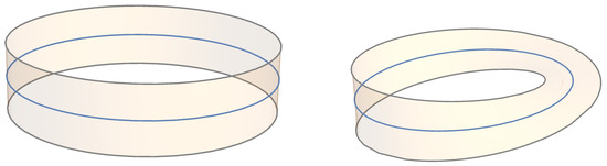
Gluing along $-\mathrm{id}$ means that $\overline{1}$ and $-\overline{1}$ are exchanged upon returning, hence returning to themselves after a second round. We may thus picture them to traverse the boundary of a Möbius band. The element $\overline{0}$, which follows the unit section, will again trace out a circle. Hence, the total space of this bundle consists of a circle and the boundary of a Möbius band, and thus is homeomorphic to two disjoint circles. It thus cannot be homeomorphic to the trivial bundle, as this consists of three disjoint circles. Compare the illustrations of the bundles in Figure 1.

Figure 1. Representatives of the two non-isomorphic classes of ${\mathbb{Z}}_3$-bundles over the circle; see Example 1. The shaded cylinder and Möbius band are visual aids. In both cases, the unit section traces out the middle circle, whereas the other group elements follow the boundary.

Observe that this example treats the most elementary non-trivial group bundle. Indeed, the circle requires at least one automorphism to be specified, and the smallest group possessing non-trivial automorphisms is ${\mathbb{Z}}_3$. Naturally, if G is trivial, then $B\cong M$ is trivial, as the fiber has only one point. In case $G={\mathbb{Z}}_2$, the bundle will also be trivial; one can use Lemma 1 to conclude that all transition functions are trivial, or alternatively use Proposition 1 to remark that B consists of two disjoint copies of M and hence is trivial.

The argument in Example 1 holds for any group G with $Aut\left(G\right)\cong {\mathbb{Z}}_2$. Indeed, the identity map in $Aut\left(G\right)$ yields the trivial bundle $S^1\times G$, while the non-identity map yields a non-trivial bundle. For instance, picking $G=\mathbb{Z}$ yields infinitely many copies of the boundaries in Figure 1. That is, either each $n\in \mathbb{Z}$ is glued to n and one obtains rings on the infinite cylinder, or each n is glued to $-n$ and one obtains rings on the infinite Möbius band.The choice $G=U\left(1\right)$ reproduces the familiar picture of a cylinder whose edge circles are glued to obtain a torus, i.e., a Klein bottle. As ${\mathbb{Z}}_4$ is naturally a subgroup of $U\left(1\right)$, the case $G={\mathbb{Z}}_4$ can again be viewed as lines on a surface, where the surface is now given by a $U\left(1\right)$-bundle. Pictorially, one places four equidistant points on a circle, which become straight lines on a cylinder, and by gluing the edge circles of this cylinder, one finds all lines coming back to themselves on the torus, i.e., two lines coming back and two lines exchanging on the Klein bottle.

A final remark is that the (isomorphism class of) a group bundle over the circle may be the same for different automorphisms of G. For one, if the automorphisms can be connected by a path, then the resulting bundles are isomorphic. As an example, if $G=\mathbb{R}$, then $Aut\left(\mathbb{R}\right)={\mathbb{R}}^{\times }\cong {\mathbb{R}}_{>0}\times {\mathbb{Z}}_2$, and the class of the obtained bundle only depends on the ${\mathbb{Z}}_2$ part. In addition, conjugate automorphisms of G also yield isomorphic bundles. This, we illustrate in Example 2.

Example 2

(${\mathbb{Z}}_2\times {\mathbb{Z}}_2$-bundles over the circle). Let us consider $G={\mathbb{Z}}_2\times {\mathbb{Z}}_2\cong \{1,a,b,c\}$, where $a^2=1$, $ab=ba=c$ and similarly for the cyclic permutations of these equations. The elements a, b and c thus satisfy identical relations, and indeed the automorphisms are given by permuting a, b and c amongst themselves. Hence, $Aut\left(G\right)$ is isomorphic to $S_3$.

Although this group has six elements, there are fewer isomorphism classes. Let us go over all permutations in $Aut\left(G\right)$. Naturally, the identity permutation will yield the trivial group bundle $S^1\times G$. All the transpositions will yield another class, as do the three cycles.

Take $\left(ab\right)$ for instance. This means that we glue the four intervals in $[0,1]\times G$ such that the intervals of a and b form a single circle, whereas the intervals of 1 and c will each form a separate circle. For $\left(bc\right)$ and $\left(ca\right)$, one will obtain essentially the same picture, revealing that the obtained bundles are isomorphic. For $\left(abc\right)$ and $\left(acb\right)$, a similar argument holds; now the intervals of a, b, and c are connected to a single circle, and the only difference between the two gluings is the order in which the pieces of the circle are traversed.

We thus see that the obtained bundle class is the same for automorphisms in the same conjugacy class of $Aut\left(G\right)$. Moreover, each conjugacy class yields another class of group bundles; the obtained spaces are homeomorphic to 4, 3, and 2 circles, respectively.

2.2. Group-Space Bundles

Let us shift our attention to group sets instead of groups. This brings us closer to principal bundles, as these are a special class of group-space bundles. Indeed, the axioms on the fiber of a principal bundle are similar to the axioms of a group set. We will investigate these objects in more detail here and later on in the paper, and so we wish to review some basic statements on group sets.

Definition 2.

Let G be a group with unit e. A G-set is a tuple $(F,A)$ where F is a set and A is a left action of G on F, i.e., a map

$$A:G\times F\to F,(g,f)\mapsto gf$$

(2)

such that $\forall f\in F$ and $\forall g_1,g_2\in G$ one has $g_1\left(g_{2}f\right)=\left(g_1{g}_2\right)f$ and $ef=f$. For convenience, we will simply refer to the G-set as F, which we understand as a set endowed with a left action A by G. In case G is a topological group, F is a topological space, and the action map A is continuous, F is called a G-space. Similarly, if G is a Lie group, F is a manifold, and the action map A is smooth, then F is a G-manifold.

A function $\alpha :F\to F^{\prime }$ between a G-set F and a $G^{\prime }$-set $F^{\prime }$ is called ξ-equivariant, where $\xi :G\to G^{\prime }$ is a homomorphism, if

$$\alpha \left(gf\right)=\xi \left(g\right)\alpha \left(f\right),\forall f\in F,\forall g\in G.$$

(3)

In particular, a G-map is a function between two G-sets that is ${\mathrm{id}}_G$-equivariant, i.e., $\alpha \left(gf\right)=g\alpha \left(f\right)$. In case F and $F^{\prime }$ are G-spaces or G-manifolds, the map α is also required to be continuous, i.e., smooth. Moreover, the category formed by G-sets and G-maps is called the category of G-sets. Similarly, one has the category of G-spaces and G-manifolds.

A G-set is called free/transitive if the action is free/transitive, which is equivalent to the map

$$\begin{array}{cc}\hfill G\times F& \to F\times F\hfill \\ \hfill (g,f)& \mapsto (gf,f)\hfill \end{array}$$

(4)

being respectively injective/surjective. Denoting the action quotient map as $q:F\to F/G$, the image of the above map, i.e., all pairs of elements in the same orbit, can be written as

$$F{\times }_{q}F=\left\{(f^{\prime },f)\in F\times F|q\left(f\right)=q\left(f^{\prime }\right)\right\}.$$

(5)

If F is both free and transitive, then F is called a principal homogeneous space for G, or G-torsor.

The fibers of a principal G-bundle are thus G-torsors. Of course, a particular G-torsor is the underlying space of G where the action is given by left translation. Clearly, any G-torsor F is isomorphic to this G-torsor; any orbit map establishes an isomorphism of G-torsors. A straightforward generalization of principal bundles is thus group-space bundles, which can be defined as follows.

Definition 3.

Let G be a topological group and F a G-space. A G-space bundle with model F is a fiber bundle $(\pi ,B,M,F)$ such that the following hold:

• Each fiber of B is a G-space. That is, there is a bundle map

  $$\begin{array}{cc}\hfill A:G\times B& \to B\hfill \\ \hfill (g,b)& \mapsto gb\hfill \end{array}$$

  (6)

  such that $(B_x,A{|}_{G\times B_x})$ is a G-space for all $x\in M$.
• Each point $x\in M$ has a neighborhood U and a homeomorphism $\varphi :U\times F\to {\pi }^{-1}\left(U\right)$ such that $\pi \circ \varphi ={pr}_U$, and for each $u\in U$, the map ${\varphi |}_{\left\{u\right\}\times F}:\left\{u\right\}\times F\to B_u$ is an isomorphism of G-spaces.

Let B be a G-space bundle and $B^{\prime }$ be a $G^{\prime }$-space bundle. A map of group-space bundles $f:B\to B^{\prime }$ is a bundle map such that ${f|}_{B_x}:B_x\to B_x^{\prime }$ is ξ-equivariant for all $x\in M$, i.e., $f\left(gb\right)=\xi \left(g\right)f\left(b\right)$ for all $g\in G$ and $b\in B$, where $\xi :G\to G^{\prime }$ is a homomorphism.

This defines the category of group-space bundles. From it, one obtains special subcategories by restricting the model group space to a prescribed class. The principal bundles are readily recognized as the restriction of group-space bundles to the case where the model fiber is a torsor. The group-space bundles are more general in the following sense.

Lemma 2.

The principal bundles are a full subcategory of the group-space bundles.

Proof. 

As a G-torsor is a G-space, any principal bundle is a group-space bundle. In addition, any map of principal bundles is a map of group-space bundles. This proves the subcategory claim. It is full, as any group-space bundle map between principal bundles is an equivariant bundle map, hence a map of principal bundles. □

A significant difference between principal bundles and general group-space bundles is the way in which the structure group can describe changes in the fiber. This is relevant already for the transition functions but also when one considers holonomy. The nature of the transition functions can be found in the standard way, as performed for group bundles previously, and results in the following.

Lemma 3.

The transition functions of a group-space bundle with model fiber F take values in the automorphism group $Aut\left(F\right)$, i.e., the group of invertible group space maps $F\to F$.

Let us first relate this back to principal G-bundles, in which case F may be taken as the G-torsor G. The left-equivariant invertible maps are exactly the right translations; hence, $Aut\left(F\right)\cong G$. In other words, the group G faithfully describes all relevant changes in the fiber F. This need not be so for general group spaces F. Intuitively speaking, if F is not free, then G has redundant elements, and if F is not transitive, then G is too small. A more formal description of $Aut\left(F\right)$ is given in Appendix A.

Another significant difference is the internal structure of the fiber F. By this, we mean that F itself can have an interesting topology. Let us consider the quotient map $q:F\to F/G$. Remarkably, if q is locally trivial, the tuple $(q,F,F/G,G)$ is itself a group-space bundle. This bundle need not be trivial; in fact, one can take F to be (the total space of) any non-trivial principal G-bundle. This means that non-trivial topology can appear not only on the global level but also already on the fiber level.

3. Semi-Torsors and Semi-Principal Bundles

3.1. Basic Properties

We are now in the position to introduce our main objects of study. As just seen, allowing general group spaces to be the model fiber of the bundle means that even fibers themselves can have non-trivial topology. We will thus restrict ourselves to a certain class of group spaces, for which the fibers have both a clear automorphism group and the quotient map is trivial. The first condition brings us to free group spaces. The second condition is fulfilled in the standard torsor case with a single orbit, but multiple orbits are still possible as long as these form a partition of the group space in open and closed subsets. That is, we arrive at G-spaces F such that F is free and $F/G$ is discrete. It readily follows that F must be isomorphic to $G\times F/G$ as G-spaces, which reveals the trivial topology. As all such G-spaces are of the form ${\bigsqcup }_{F/G}G$, i.e., a disjoint union of ‘standard’ torsors, we propose to call them semi-torsors. We will start phrasing the results for manifolds, and leave the topological equivalents as implicit.

Definition 4.

Let G be a Lie group and F a G-manifold. Then, F is a semi-torsor if F is free and $F/G$ is discrete.

Clearly, every torsor is a semi-torsor—they form the case where $F/G$ consists of a single point. As principal bundles correspond to torsors, the bundles corresponding to the semi-torsors will form a generalization of the principal bundles. We call these bundles semi-principal bundles, as they locally look like a sum of principal bundles. We define these in the following definition. A schematic overview of how these bundles relate to group spaces and other classes of bundles can be found in Figure 2.

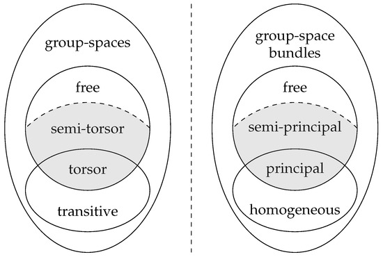
Figure 2. Correspondence between classes of group spaces and the classes of group-space bundles having these as fibers. This paper focuses on the gray parts, i.e., the semi-torsors and semi-principal bundles, which extend the torsors and principal bundles.

Definition 5.

Given a Lie group G, a semi-principal G-bundle is a group-space bundle $\pi :B\to M$, where the model fiber F is a G-semi-torsor. That is, B is endowed with a fiber-preserving G-action, local trivializations of B are G-equivariant, and the model fiber F is a free G-manifold such that $F/G$ is discrete.

Unlike principal bundles, the projection map $\pi :B\to M$ of a semi-principal bundle need not coincide with the action quotient $Q:B\to B/G$, where $B/G$ is endowed with the unique smooth manifold structure such that Q becomes a surjective submersion. Indeed, when taking the action quotient, the fiber F is reduced to $F/G$, which need not consist of a single point. Nevertheless, this new fiber is a discrete space, and as proven below, $B/G$ forms a covering of M. As Q will still define a principal bundle, the following result says that any semi-principal G-bundle is a principal G-bundle on top of a covering space.

Proposition 2.

Let $\pi :B\to M$ be a semi-principal G-bundle with model fiber F, set $X=F/G$. The map $Q:B\to B/G$ defines a principal G-bundle. Moreover, the quotient space $B/G$ is itself an X-bundle over M, i.e., a regular $\left|X\right|$-fold covering. This bundle is defined by the reduced map $\pi /G:B/G\to M$ given by the relation $\pi =\pi /G\circ Q$, i.e.,

(7)

is a commutative diagram of semi-principal bundles.

Proof. 

As $\pi$ is G-invariant, it is constant on the fibers of Q. As Q is a smooth submersion, the map $\pi /G$ is a well-defined smooth map [5] (Thm 4.30). To see the local forms of Q and $\pi /G$, let us use a G-equivariant local trivialization ${\varphi :U\times X\times G\to B|}_U$ of $\pi$. One can reduce $\varphi$ to orbits, and as $\left(B{|}_U\right)/G=(B/G){|}_U$, this results in the commutative diagram

(8)

where all solid arrows are smooth.

Let us consider the induced map $\varphi /G$. It is smooth, as $Q\circ \varphi$ is a smooth map that is constant on the fibers of the smooth submersion ${pr}_{U\times X}$. In fact, $\varphi /G$ is a diffeomorphism. Being the quotient of a bijection, it is bijective. Its inverse is smooth as well; ${pr}_{U\times X}\circ {\varphi }^{-1}$ is a smooth map that is constant on the fibers of the smooth submersion Q. Hence, $\varphi /G$ is a local trivialization of $\pi /G$ provided that $\pi /G\circ \varphi /G={pr}_U$. The latter can be deduced from

$$(\pi /G\circ \varphi /G)(u,x)=(\pi /G\circ Q\circ \varphi )(u,x,g)=(\pi \circ \varphi )(u,x,g)={pr}_U(u,x,g)=u,$$

(9)

where $g\in G$ may be chosen arbitrarily because of G-equivariance. Hence, $\pi /G$ is an X-bundle over M, and as X is discrete, this is a covering.

We then turn our attention to $Q:B\to B/G$. Using the same maps as above, one can find a local trivialization for Q, namely, $\varphi \circ ((\varphi /G^{-1}\times {\mathrm{id}}_G):(B/G){|}_U\times G\to B{|}_U$, $(\left[b\right],g)\mapsto \varphi ({(\varphi /G)}^{-1}\left(\left[b\right]\right),g)$. As $\varphi$ is G-equivariant, so is this diffeomorphism, and as it satisfies

$$\begin{array}{cc}\hfill Q\circ \left[\varphi \circ (\varphi /G^{-1}\times {\mathrm{id}}_G)\right]& =\varphi /G\circ {pr}_{U\times X}\circ (\varphi /G^{-1}\times {\mathrm{id}}_G)\hfill \\ \hfill & =\varphi /G\circ \varphi /G^{-1}\circ {pr}_{{(B/G)|}_U}={pr}_{{(B/G)|}_U}\hfill \end{array}$$

(10)

it is a local trivialization of Q. This implies Q is a principal G-bundle. □

This result clearly reveals two special cases of semi-principal bundles. Naturally, one case is where the bundle is actually principal, which means that $\pi$ and Q coincide. The other special case is that $\pi$ and $\pi /G$ coincide, which happens if and only if G is trivial. Here, the definition of the semi-principal bundle reduces to that of a fiber bundle with discrete fiber, i.e., a regular covering space.

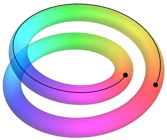
An example of a generic semi-principal bundle can be found in Example 3 below. Here, we consider the trivial principal $U\left(1\right)$-bundle over the circle $S^1$, i.e., the torus, but we wind it around multiple times to obtain a coil-like object. The resulting projection is no longer a principal bundle, but it does remain semi-principal. We will repeatedly build upon this example throughout the paper.

Example 3

(Winding torus). Let us consider the torus $T^2=S^1\times S^1$, endowed with the standard $U\left(1\right)$-action on its second factor. The projection $\pi :T^2\to S^1$ on the first factor then realizes the torus as a trivial principal $U\left(1\right)$-bundle over the circle. However, we can also view $T^2$ as a semi-principal bundle over $S^1$ in the following way.

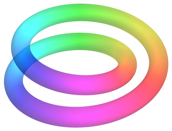
Consider the map $s_k:S^1\to S^1$, with $k\ge 1$ as an integer, given by winding the circle k times around, i.e., $z\mapsto z^k$ for z on the unit circle in $\mathbb{C}$. Then, ${\Pi }_k:=s_k\circ \pi :T^2\to S^1$ winds the torus k times around the circle. The picture to have in mind is illustrated in Figure 3 for the case $k=2$. Clearly, ${\Pi }_k$ defines a semi-principal $U\left(1\right)$-bundle with model fiber ${\bigsqcup }^k{S}^1$, i.e., k disjoint circles. For $k>1$, so that ${\Pi }_k\ne \pi$, the bundle ${\Pi }_k$ is non-trivial as can be deduced using topology. Namely, the trivial semi-principal $U\left(1\right)$-bundle over $S^1$ with model fiber ${\bigsqcup }^k{S}^1$ is given by the projection $S^1\times \left({\bigsqcup }^k{S}^1\right)\to S^1$ on the first factor, so that in particular the total space consists of k disjoint tori. As the total space of ${\Pi }_k$ is always a single torus, it follows that ${\Pi }_k$ is non-trivial for $k>1$.

Figure 3. Illustration of the bundle ${\Pi }_2$ in Example 3. This space is topologically a torus, but the projection ${\Pi }_2$ indicates that it winds twice around its base circle. Points with the same color are projected to the same point in $S^1$.

We now move to the observation that semi-principal bundles admit parallel transport in almost exactly the same way as principal bundles do. We will first prepare ourselves for this theory by studying connections that are compatible with the group action, leading to a generalization of the Maurer–Cartan form on semi-torsors. After this, we will show how such connection forms define parallel transport on semi-principal bundles.

3.2. Group Compatible Connections and a Generalization of the Maurer–Cartan Form

Parallel transport is conveniently described using connection 1-form, so let us start by considering the appropriate 1-forms for semi-torsors and semi-principal bundles. One way of writing the axioms for a 1-form $\omega$ to be a principal connection is by assuming two relations involving the G-action on the manifold. In other words, these axioms do not need to know more than a G-manifold structure. Let us write the action map as $A:G\times F\to F$, where acting with g is denoted as $L_g:=A(g,-):F\to F$. One can also consider a specific point $f\in F$, and restrict A to $A_f:=A(-,f):G\to F$. The differential $a_f={\left(d{A}_f\right)}_e:\mathfrak{g}\to T_{f}F$, where $\mathfrak{g}$ again denotes the Lie algebra of G, is known as the infinitesimal action at f. We now have the notation to state the following definition, using only the two standard axioms of a principal connection.

Definition 6.

Let G be a Lie group with algebra $\mathfrak{g}$ and let F be a (left) G-manifold. A $\mathfrak{g}$-valued 1-form ω on F is called a G-connection 1-form, or just G-connection, if

• ${\omega }_f\circ a_f={\mathrm{id}}_{\mathfrak{g}}$ for all $f\in F$,
• ${\left(L_g\right)}^{\ast }\omega ={Ad}_g\left(\omega \right)$ for all $g\in G$.

As this definition only concerns the G-manifold structure, it readily applies to semi-principal and principal bundles. For these cases, one also evades the following technical issue. Namely, a G-connection need not exist for an arbitrary G-manifold. The left-inverse axiom of ${\omega }_f$ implicitly states that $a_f$ will be a right-inverse; hence, $a_f$ must be injective for all $f\in F$. In other words, the action has to be free on a local level. Again, we will not treat the general theory but consider the case of semi-principal bundles. We remark that we choose the name G-connection to avoid confusion. As Proposition 2 indicates, a G-manifold can be a principal bundle for one bundle projection and a semi-principal bundle for another. The axioms of a G-connection 1-form do not make reference to such differences; hence, we wish to avoid terminology suggesting such reference.

The case of a G-connection on a G-semi-torsor F turns out to be special. In this case, F admits exactly one G-connection. The key observation is that if the infinitesimal action is invertible, then the G-connection is fixed.

Proposition 3.

Any G-semi-torsor F has a natural G-connection ω given by

$${\omega }_f=a_f^{-1}.$$

(11)

Moreover, this is the only G-connection on F.

Proof. 

As the action is free, $a_f$ is injective for all $f\in F$. As $F/G$ is discrete, $dim\left(F\right)=dim\left(G\right)$; hence, $a_f$ is a linear isomorphism. Hence, the condition ${\omega }_f\circ a_f={\mathrm{id}}_{\mathfrak{g}}$ uniquely specifies ${\omega }_f=a_f^{-1}$. To verify that $\omega$ is a G-connection, it remains to check the equivariance. This reads, with Y a tangent vector in $T_{f}F$,

$${\left(L_g^{\ast }\omega \right)}_f\left(Y\right)=a_{gf}^{-1}\left(d{L}_g\left(Y\right)\right)={Ad}_g\left(a_f^{-1}\left(Y\right)\right)={Ad}_g\left({\omega }_f\left(Y\right)\right),$$

(12)

where we use the relation $d{L}_g\circ a_f=a_{gf}\circ {Ad}_g$. □

This 1-form can be considered an extension of (a left-action version of) the usual canonical 1-form on G, also known as the Maurer–Cartan form [6]. A crucial difference is that the above form $\omega$ does not need any identification of (a part of) F with G. Moreover, in case F is G viewed as a (left) G-torsor, one does obtain the usual formula. Indeed, then $A_g=R_g$ and one finds

$${\omega }_g=a_g^{-1}={\left(d{A}_g\right)}_e^{-1}={\left(d{R}_g\right)}_e^{-1}={\left(d{R}_{g^{-1}}\right)}_g$$

(13)

which is indeed the Maurer–Cartan form in the case of a left-action.

Another perspective on this connection involves the map

$$\begin{array}{cc}\hfill G\times F& \to F{\times }_{q}F\hfill \\ \hfill (g,f)& \mapsto (gf,f)\hfill \end{array}$$

(14)

which by choice of image is always surjective. For a free action, this map is also injective, and an inverse function exists. It is even a diffeomorphism; the dimensions of the source and target space coincide, and the differential has full rank. Let us write the smooth inverse as

$$\begin{array}{cc}\hfill F{\times }_{q}F& \to G\times F\hfill \\ \hfill (f^{\prime },f)& \mapsto ([f^{\prime }/f],f)\hfill \end{array}$$

(15)

where $[-/-]:F{\times }_{q}F\to G$ is the smooth map sending $(f^{\prime },f)$ to the unique element $[f^{\prime }/f]\in G$ such that $f^{\prime }=[f^{\prime }/f]f$. That is, the division map allows one to track the group element relating points in F. Its derivative will thus yield an infinitesimal generator, which yields again the unique G-connection on F in the following way.

Proposition 4.

The canonical G-connection on a G-semi-torsor F can alternatively be written as

$${\omega }_{\gamma \left(0\right)}\left(\dot{\gamma }\left(0\right)\right)=\frac{d}{dt}{|}_{t=0}[\gamma \left(t\right)/\gamma \left(0\right)],$$

(16)

where $\gamma :(-ϵ,ϵ)\to F$ is a curve in F.

Proof. 

As $dim\left(F\right)=dim\left(G\right)$, $\gamma \left(t\right)$ and $\gamma \left(0\right)$ always lie in the same orbit; hence, the stated division is well defined. It suffices to check the G-connection axioms; in fact, the left-inverse property alone is already sufficient according to Proposition 3. Taking $f\in F$ and $Y\in \mathfrak{g}$, this verification reads

$${\omega }_f\left(a_f\left(Y\right)\right)=\frac{d}{dt}{|}_{t=0}[exp\left(tY\right)f/f]=\frac{d}{dt}{|}_{t=0}exp\left(tY\right)=Y.$$

(17)

The equivariance can also be verified using the identity $[g{f}^{\prime }/gf]=g[f^{\prime }/f]g^{-1}=C_g\left([f^{\prime }/f]\right)$:

$$\begin{array}{cc}\hfill {\left(L_g^{\ast }\omega \right)}_{\gamma \left(0\right)}\left(\dot{\gamma }\left(0\right)\right)& =\frac{d}{dt}{|}_{t=0}[g\gamma \left(t\right)/g\gamma \left(0\right)]\hfill \\ \hfill & =\frac{d}{dt}{|}_{t=0}{C}_g\left([\gamma \left(t\right)/\gamma \left(0\right)]\right)={Ad}_g\left({\omega }_{\gamma \left(0\right)}\left(\dot{\gamma }\left(0\right)\right)\right).\hfill \end{array}$$

(18)

□

The semi-torsor assumption cannot be omitted; the points $\gamma \left(t\right)$ and $\gamma \left(0\right)$ should be in the same orbit for any path $\gamma$, and hence the dimensions of F and G should be equal. Of course, here we still assume the action to be free; otherwise, the division would be ill defined. Hence, F can only consist of separated copies of the standard G-torsor, meaning F is a G-semi-torsor.

Again, this notation reduces to (the left-action version of) the Maurer–Cartan form in case F is the G-torsor G. This time, the key relation is $[-/g]=R_{g^{-1}}$, so for a curve $\gamma$ such that $(\gamma ,\dot{\gamma })\left(0\right)=(g,Y)$ it holds that

$${\omega }_g\left(Y\right)=\frac{d}{dt}{|}_{t=0}[\gamma \left(t\right)/g]=\frac{d}{dt}{|}_{t=0}{R}_{g^{-1}}\left(\gamma \left(t\right)\right)=d{R}_{g^{-1}}\left(Y\right).$$

(19)

Nevertheless, the division map does not need to employ a right translation, making it more general.

Example 4

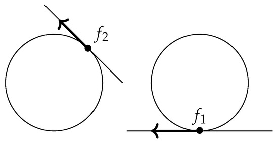
(Connection on disjoint circles). Let us illustrate the connection for the $U\left(1\right)$-set $F=S^1\bigsqcup S^1$. Pick a point $f\in F$. The infinitesimal action $a_f:\mathbb{R}\to T_{f}F$ basically identifies the tangent line at f with $\mathbb{R}$. Hence, there is a canonical way to associate any tangent vector to a number, which gives the 1-form ω. This association is illustrated in Figure 4.

Figure 4. At each point f in F, the infinitesimal action $a_f$ identifies $T_{f}F$ (here, the tangent line) with the Lie algebra (here $\mathfrak{u}\left(1\right)\cong \mathbb{R}$). A tangent vector thus canonically corresponds to a unique algebra element.

3.3. Parallel Transport on Semi-Principal Bundles

The next step is to demonstrate that a G-connection on a semi-principal G-bundle induces a G-equivariant parallel transport. In other words, we wish to show that this property of principal bundles extends to all semi-principal bundles. One can prove this in various ways. One way is to use the observation that a semi-principal bundle locally looks like the projection $U\times G\times X\to U$, which locally looks like the principal projection $U\times G\to U$, hence allowing for a similar argument to principal bundle theory. Alternatively, one can use the result on principal bundles and extend it using the decomposition from Proposition 2. Let us employ the latter method in the following proof.

Proposition 5.

A semi-principal G-bundle with a G-connection admits G-equivariant parallel transport.

That is, let $\pi :B\to M$ be a semi-principal G-bundle and ω a G-connection on B. Given any piecewise smooth curve $\gamma :[0,1]\to M$ and an initial point $b\in B$ above $\gamma \left(0\right)$, there is a unique horizontal lift $\Gamma :[0,1]\to B$ through b, specified by $\pi \circ \Gamma =\gamma$ and $\Gamma \left(0\right)=b$. Moreover, the lift of γ starting from $gb$ is $g\Gamma$. In particular, the parallel transport map $P_{\gamma }:B_{\gamma \left(0\right)}\to B_{\gamma \left(1\right)}$ given by $b\mapsto \Gamma \left(1\right)$ is well defined and G-equivariant.

Proof. 

By Proposition 2, the semi-principal bundle $\pi :B\to M$ decomposes as a principal G-bundle $B\to B/G$ and a covering $B/G\to M$. Lifting the curve $\gamma$ from M to a curve $\overline{\gamma }$ in $B/G$ with initial point $\left[b\right]=Gb$ then follows from covering theory. Now, $\omega$ is a G-connection, hence a principal connection concerning the principal G-bundle $B\to B/G$. As b lies above $Gb$, one can lift $\overline{\gamma }$ to a unique $\Gamma$ in B such that $\Gamma \left(0\right)=b$. Hence, any curve $\gamma$ in M lifts to a unique curve $\Gamma$ in B given an initial condition and the 1-form $\omega$. If the starting point is $gb$, then only the lifting from $B/G$ to B changes. However, as $B\to B/G$ is a principal bundle, the lift becomes $g\Gamma$ as claimed. □

We have thus demonstrated that the parallel transport maps $P_{\gamma }$ are well defined and G-equivariant, but there is a crucial difference with respect to parallel transport on principal bundles. Namely, on semi-principal bundles, $P_{\gamma }$ need not return a point to the same group orbit. Principal bundles guarantee this by having a single group orbit as fiber, but for semi-principal bundles, this is not so. The group action is thus not sufficient to express the map $P_{\gamma }$ with. This brings us to the main difference between the parallel transport on principal and more general semi-principal bundles: although both have well-defined and equivariant parallel transport, the holonomy on semi-principal bundles need not be expressible with a group element. An illustration of this in provided in Example 5. This phenomenon provides the main motivation for the study of bases in the coming sections.

Example 5.

We have already seen the torus $T^2=S^1\times S^1$ as a $U\left(1\right)$-bundle by acting on the second factor. Decomposing the torus like this, a $U\left(1\right)$-connection on $T^2$ is obtained by declaring that a path is horizontal if it has a constant second factor. This $U\left(1\right)$-connection is then compatible with all of the projections ${\Pi }_k:T^2\to S^1$.

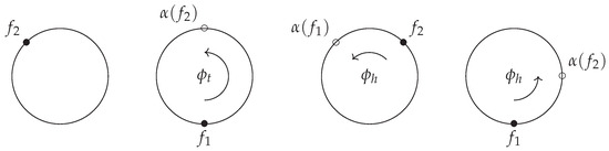
When the bundle is semi-principal, in particular, for $k=2$, the parallel transport will contain the following. Let γ be a path in the base $S^1$ that makes a single turn. As seen in Figure 5, its lift Γ will end up in the original fiber but in a different circle/orbit as before. Consequently, the points $\Gamma \left(0\right)$ and $\Gamma \left(1\right)$ cannot be related by an element of $U\left(1\right)$. This picture is also close to the physical setting of adiabatic quantum mechanics, where states with a $U\left(1\right)$-phase freedom can be exchanged upon traversing a loop, i.e., $S^1$. The parallel transport cannot be described by a phase factor alone.

Figure 5. Example of parallel transport on the double torus. The path is well defined, and translating the initial point yields the translated lift as usual. However, as the final point lies in another orbit within the fiber, this holonomy cannot be expressed with an element of $U\left(1\right)$.

4. Bases of a Group Set

In this section, we will introduce and study the notion of the basis, also called frame, of a group set. This will include the study of the space formed by all the frames of a group set and its symmetry group, which will be a wreath product. We can then demonstrate how maps of semi-torsors can be expressed in matrix form using such a basis. To finish, we inspect how going from a semi-torsor to its torsor of frames defines a functor.

4.1. Basis of a Group Set

Similar to the notion of basis of a vector space, one can define the basis of a G-set F. Intuitively speaking, such a basis should be a tuple ${\left(f_x\right)}_{x\in X}$ of elements of F, where X is the indexing set such that any point in F can be ‘reached’ using these points in a unique way, and that a G-map from F to any other G-set is specified once the images of the $f_x$ are known. We will use that a tuple ${\left(f_x\right)}_{x\in X}$ is equivalent to a function $\tilde{f}:X\to F$ by the relation $\tilde{f}\left(x\right)=f_x$, and we will often use the $\tilde{f}$ formalism throughout this paper for convenience. We will use tilde notation to indicate tuples throughout this paper.

Let us first discuss how this ‘reaching of points’ can be phrased in a formal way, staying in close analogy to vector spaces. In linear algebra, if V is a real vector space, then given a tuple $\tilde{v}:=(v_1,\dots ,v_m)$ of vectors in V, there is the associated map from coefficients to the vector space as

$$\begin{array}{cc}\hfill {\varphi }_{\tilde{v}}:{\mathbb{R}}^m& \to V\hfill \\ \hfill (c_1,\dots ,c_m)& \mapsto \sum _{i=1}^m{c}_i{v}_i.\hfill \end{array}$$

(20)

As this map is already linear, it is an isomorphism of vector spaces if and only if it is bijective. This question is usually subdivided in the properties of linear independence and spanning set. That is, the tuple $\tilde{v}$ is linearly independent if and only if ${\varphi }_{\tilde{v}}$ is injective, and similarly, the tuple is a spanning set if and only if ${\varphi }_{\tilde{v}}$ is surjective. If V admits a finite basis, then all bases of V have the same number of vectors, and the dimension of V is defined to be this finite number. If not, then V is called infinite dimensional.

This argument can be copied almost completely once we agree on a specific G-map induced by a tuple ${\left(f_x\right)}_{x\in X}$ of G-set elements. A G-set will in general not supply us with an addition +, but there is some sort of scaling given by the group action: $(g,f)\mapsto gf$. It is now straightforward to extend this map to tuples; we define this map below and also extend the definition of a basis to G-sets. Here, we agree on the canonical G-set structure on $G\times X$ given by the action $g(h,x)=(gh,x)$.

Definition 7.

Let X be an index set, and consider the set $F^X$ of functions $\tilde{f}:X\to F$, or equivalently the set of ordered tuples ${\left(f_x\right)}_{x\in X}$ with $f_x\in F$ for all $x\in X$. Given such a tuple, we define its associated map to be the G-map

$$\begin{array}{cc}\hfill {\varphi }_{\tilde{f}}:G\times X& \to F\hfill \\ \hfill (g,x)& \mapsto g·f_x=g·\tilde{f}\left(x\right).\hfill \end{array}$$

(21)

A tuple $\tilde{f}$ is called a basis of F if the associated map ${\varphi }_{\tilde{f}}$ is an isomorphism of G-sets. The subset of $F^X$ consisting of all bases of F we denote as $Fr\left(F\right)$.

Let us first illustrate this definition in some simple cases, prior to delving into further properties. To start, in case F is a finite set—canonically a G-set for G the trivial group $\left\{e\right\}$—one finds that the bases of F are just the set $F!$ consisting of all tuples that list all elements of F exactly once. This illustrates a factorial dependence on the number of orbits, which is a general fact. It also motivates our use of the factorial symbol ! in some future constructions. We then provide a simple example with non-trivial G.

Lemma 4.

For F a finite set, viewed as a group set under the trivial group,

$$Fr\left(F\right)=F!:=\left\{\mathit{tuples}\mathit{listing}\mathit{all}\mathit{elements}\mathit{of}\mathit{F}\mathit{exactly}\mathrm{once}\right\}.$$

(22)

Proof. 

For G, the trivial group, the map ${\varphi }_{\tilde{f}}$ reduces to $\tilde{f}$. If F has n elements, pick $X=I_n:=\{1,2,\dots ,n\}$. The map $\tilde{f}$ is an isomorphism if and only if it is bijective, meaning its associated tuple $(f_1,\dots ,f_n)$ should yield any given point of F exactly once. □

Example 6

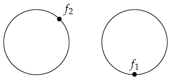
(Frames of two circles). Let us consider a simple case. Let us take $G=U\left(1\right)$, and $F=S^1\bigsqcup S^1$ two disjoint circles. Physically, this can represent two distinct eigenstates, which are determined only up to the usual $U\left(1\right)$ phase factor. We draw the circles in the plane, and use the convention that G rotates positively, i.e., counterclockwise. Given any point $f\in F$, the group action will take us to any point on the same circle, but the other circle is out of reach. We thus need two points $f_1$ and $f_2$, one for each circle, in order to reach any point in F using the group action, e.g., those in Figure 6. This we can write in the above style by having $X=I_2:=\{1,2\}$, where indeed

$$\begin{array}{cc}\hfill {\varphi }_{(f_1,f_2)}:U\left(1\right)\times I_2& \to S^1\bigsqcup S^1\hfill \\ \hfill (g,i)& \mapsto g·f_i\hfill \end{array}$$

(23)

is an isomorphism of $U\left(1\right)$-sets, even of $U\left(1\right)$-manifolds.

Figure 6. In case of the $U\left(1\right)$-set $S^1\bigsqcup S^1$, a frame consists of a pair of points $(f_1,f_2)$, one for each circle/orbit. The circles neither carry preferred points nor any order amongst themselves; these only come after choosing a frame.

In Figure 6, we label the circle on the right as circle 1, and the circle on the left as circle 2—neither circle has an intrinsic label, and any label is an external choice. Notice that the number of possible labels grows factorially in the number of circles.

Before discussing the existence of these bases, let us first consider the following. Namely, the scaling of vector spaces may differ in a crucial way from the group action used here. If one wants to preserve some idea of linear independence, it is important that $g_{1}f=g_{2}f$ implies $g_1=g_2$ for generic f. However, this need not hold for a general group action; it holds only for free actions. Hence, one may expect that the idea of a basis only matches intuition when F is free. This is indeed sufficient; the map ${\varphi }_{\tilde{f}}$ is an isomorphism if and only if it is bijective, so we need both injectivity and surjectivity. The map ${\varphi }_{\tilde{f}}$ is surjective if and only if every orbit contains at least one of the $f_x$, and if F is free, then ${\varphi }_{\tilde{f}}$ is injective if and only if the $f_x$ lie in different orbits. This indeed mimics the properties of linear independence and spanning set. In fact, having a basis and being free is equivalent as stated in the following lemma. We also prove the intuitive statement that all bases of a given G-set have the same cardinality; this ‘dimension’ is now the number of orbits $|F/G|$, which can be infinite.

Lemma 5.

A G-set F has a basis if and only if F is free. Moreover, for a free G-set F, the index set X is unique up to bijection, in particular, $X\cong F/G$.

Proof. 

If F has a basis, then $F\cong G\times X$ as G-sets. As the latter is free, so is F. Conversely, assume F is free. Then, every orbit in F is bijective to G. We only need to specify base points for each orbit; these base points will form the basis. That is, for each orbit $x\in F/G$, pick a point in this orbit and denote it by $s\left(x\right)$. This defines a section s of the quotient map $q:F\to F/G$. To check that s is a basis of F, we consider its induced map ${\varphi }_s:G\times F/G\to F$ given by $(g,x)\mapsto gs\left(x\right)$. This has an explicit inverse

$$f\mapsto \left(\right[f/s\left(q\right(f\left)\right)],q(f\left)\right),$$

(24)

where $[f/s(q\left(f\right)\left)\right]\in G$ is the group element such that $f=[f/s(q\left(f\right)\left)\right]s\left(q\right(f\left)\right)$. This element is well defined; it exists, as f and $s\left(q\right(f\left)\right)$ lie in the same orbit, and it is unique, as F is free. Hence, s is a basis of F with index set $X=F/G$.

Assuming F is free, pick two bases ${\tilde{f}}_1$ and ${\tilde{f}}_2$ with index sets $X_1$ and $X_2$, respectively. Then, ${\varphi }_{{\tilde{f}}_2}^{-1}{\varphi }_{{\tilde{f}}_1}:G\times X_1\to G\times X_2$ is a G-isomorphism. Hence, the orbit sets are bijective, which yields $X_1\cong X_2$. Hence, all index sets of the G-set F are bijective. We just saw that $F/G$ is always an index set; hence, any other index set X must be bijective to $F/G$. □

Given this result, we will restrict ourselves to free F from now on. Also, we take $X=F/G$ but sometimes still write X for clarity. In addition, one may observe that in the previous proof, one does need s to be a section; an orbit may be sent to a point in another orbit as long as all orbits are visited exactly once. We like to emphasize this freedom at certain places by not using the quotient notation.

We remark that ${\varphi }_{\tilde{f}}$ has an interesting interpretation concerning the model of a G-set. Given a finite-dimensional real vector space V, one often identifies it with ${\mathbb{R}}^m$ for some m using a linear isomorphism. In this way, the vector spaces ${\mathbb{R}}^m$, $m\in \mathbb{N}$, provide models for real (finite-dimensional) vector spaces. One may then ask what the model space is in case of G-sets, and the above indicates that this is $G\times X$. This is valid for free G-sets, as any free F is isomorphic to $G\times F/G$, hence being of the correct form. The bases are then the labels of such isomorphisms $F\cong G\times X$.

We finish this inspection of individual bases with the following statements on G-maps in relation to bases. Again, we emphasize the similarity with the theory of vector spaces.

Lemma 6.

Let $F,F^{\prime }$ be G-sets and $\alpha :F\to F^{\prime }$ a G-map. Then, we have the following:

1. 

For any $\tilde{f}\in F^X$, one has ${\varphi }_{\alpha \left(\tilde{f}\right)}=\alpha \circ {\varphi }_{\tilde{f}}$;

2. 

If F is free, the map α is fully determined by its values on a basis;

3. 

If both F and $F^{\prime }$ are free, then α is an isomorphism if and only if α sends a basis to a basis.

Proof. 

For the first, observe ${\varphi }_{\alpha \left(\tilde{f}\right)}(g,x)=g\alpha \left(f_x\right)=\alpha \left(g{f}_x\right)=\alpha \circ {\varphi }_{\tilde{f}}(g,x)$, which indeed yields ${\varphi }_{\alpha \left(\tilde{f}\right)}=\alpha \circ {\varphi }_{\tilde{f}}$. For the second, assume $\beta :F\to F^{\prime }$ is another G-map that coincides with $\alpha$ on a basis $\tilde{f}$ of F. Pick any $f\in F$; it is related to the basis $\tilde{f}$ via $f=h{f}_x$ for some $h\in G$ and $x\in X$. Using this decomposition, one finds

$$\alpha \left(f\right)=\alpha \left(h{f}_x\right)=h\alpha \left(f_x\right)=h\beta \left(f_x\right)=\beta \left(h{f}_x\right)=\beta \left(f\right)$$

(25)

and as f is arbitrary, $\alpha =\beta$. The third then follows as well; given that ${\varphi }_{\tilde{f}}$ is a G-isomorphism, then $\alpha$ is a G-isomorphism if and only if ${\varphi }_{\alpha \left(\tilde{f}\right)}$ is, i.e., if and only if $\alpha \left(\tilde{f}\right)$ is a basis of $F^{\prime }$. □

4.2. The Space of Bases of a Group Set

We will now shift our scope and study the properties of the bases of F as a whole, i.e., we study $Fr\left(F\right)$. This we do using a kind of basis criterion in terms of the quotient map q. Basically, we pose the question when a candidate basis $\tilde{f}$, i.e., any element in $F^X=\{\tilde{f}:X\to F\}$ for a chosen index set X bijective to $F/G$, lies in $Fr\left(F\right)$.

The basic observation is that the invertibility of ${\varphi }_{\tilde{f}}$, as it is equivariant, can be deduced by just knowing how the elements $f_x$ are distributed over the orbits of F, i.e., by knowing the map $q\circ \tilde{f}:X\to F/G$. More explicitly, $q\circ \tilde{f}$ fits in the commutative diagram

(26)

which indicates that $q\circ \tilde{f}$ is ${\varphi }_{\tilde{f}}$ reduced to orbits. This yields the following criterion for a candidate tuple to be a basis.

Lemma 7.

Let F be a free G-set. Then, $\tilde{f}\in F^X$ is a basis if and only if $q\circ \tilde{f}$ is bijective.

Proof. 

First, observe that ${\varphi }_{\tilde{f}}$ is injective if and only if $\tilde{f}$ reaches every orbit at most once. In other words, every fiber of q contains at most one element of the basis $\tilde{f}$. This is equivalent to $q\circ \tilde{f}$ being injective. Dually, the map ${\varphi }_{\tilde{f}}$ is surjective if and only if every orbit is reached at least once. In other words, every fiber of q contains at least one element of the basis $\tilde{f}$. This is equivalent to $q\circ \tilde{f}$ being surjective. □

Hence, the question of whether a particular $\tilde{f}\in F^X$ lies in $Fr\left(F\right)$ can be answered by inspecting whether $q\circ \tilde{f}$ is bijective. We are thus inclined to look at the map $\tilde{f}\mapsto q\circ \tilde{f}$, which we formally write as

$$\begin{array}{cc}\hfill q^X:F^X& \to X^X\hfill \\ \hfill \tilde{f}& \mapsto q\circ \tilde{f}.\hfill \end{array}$$

(27)

In other words, this map is the X-fold product of q. We may thus write Lemma 7 as the following pre-image statement.

Corollary 1.

Let F be a free G-set, set $X=F/G$, and denote by $Sym\left(X\right)$ the group of bijections of X. The set $Fr\left(F\right)$ inside $F^X$ is the pre-image of $Sym\left(X\right)$ under $q^X$.

We remark that the set $Sym\left(X\right)$ is a special subset of $X^X$; the latter has a natural monoid multiplication given by composition, and $Sym\left(X\right)$ is the set of units of this monoid.

We will now start to take topology into account; we assume G is a topological group and F is a G-space. The set $F/G$ thus inherits the quotient topology such that q is continuous. For any set X, $F^X$ inherits the product topology, and the map $q^X$ is continuous. In this setting, Corollary 1 can be used to deduce some topological properties of $Fr\left(F\right)$. This requires us to consider the topology of X, which should be homeomorphic to the topology of $F/G$ given the bijectivity from Lemma 5. We will restrict ourselves to discrete X, i.e., F should be a semi-torsor; this preserves the index set intuition and guarantees that the previous results on G-sets are still valid. Pictorially, this means that the orbits inside F form a partition of F into open and closed subsets. Under this assumption, the following holds.

Corollary 2.

If F is a G-semi-torsor, then $Fr\left(F\right)$ is open and closed in $F^X$.

Proof. 

As X is discrete, so is $X^X$ (with the product topology). Hence, $Sym\left(X\right)$ is an open and closed subset of $X^X$. As $q^X$ is continuous, the claim follows from Corollary 1. □

In case G is a Lie group and F is a G-manifold, this corollary implies that $Fr\left(F\right)$ is an open and closed submanifold of $F^X$. We assume G to be finite-dimensional in this paper, but as we allow for infinite X, the manifold $F^X$ can be infinite dimensional.

We remark that the similar version of Corollary 2 for vector spaces need not hold. For V, a real vector space of finite dimension n, this statement would be that the set $Fr\left(V\right)$ inside $V^n$ is open and closed. However, $Fr\left(V\right)$ is only an open subset of $V^n$. This can be proven by observing that $Fr\left(V\right)$ inside $V^n$ is similar to $GL(n,\mathbb{R})$ inside the space of all real $n\times n$ matrices. Now $GL(n,\mathbb{R})$ is the pre-image ${det}^{-1}(\mathbb{R}\setminus \left\{0\right\})$ and so open. It is not closed; there are sequences of invertible matrices that converge to a non-invertible matrix. This argument does not hold in the case of G-spaces if we assume that the orbits are disjoint. Given a sequence ${\tilde{f}}_k$ of bases, look at the induced sequence $q\circ {\tilde{f}}_k$ of orbit-representatives in X. As X is discrete, a sequence in X converges if and only if it becomes constant. That is, if the original sequence ${\tilde{f}}_k$ converges, then the basis elements settle in particular orbits, which must be different. As the orbits are disjoint, also the limit of the ${\tilde{f}}_k$ has basis elements in different orbits. That is, the limit of the bases ${\tilde{f}}_k$ is itself a basis.

Let us consider the frame of the $U\left(1\right)$-set given by disjoint circles as needed for the winding torus. It is clear that the set of frames is homeomorphic with a product of the group times the permutation group of the orbit space X. This is generally true as we will prove in the following section.

Example 7.

We defined in Example 3 the bundle ${\Pi }_k:T^2\to S^1$ with model fiber ${\bigsqcup }^k{S}^1$. This model fiber can also be viewed as $S^1\times I_k$, i.e., we pick an arbitrary ordering of the circles for our convenience. A frame of $S^1\times I_k$ is then a tuple ${\left((z_j,i_j)\right)}_{j=1}^k$, with $z_j\in S^1$ and $i_j\in I_k$ such that $j\mapsto i_j$ is a permutation of $I_k$. Concerning its topological properties, we see that varying the $z_j$ yields a k-dimensional torus $T^k:={\prod }^k{S}^1$. Furthermore, one obtains such a torus for any permutation of $I_k$, i.e., the tori can be indexed by the permutation group $Sym\left(I_k\right)=S_k$. This means that $Fr(S^1\times I_k)$ is homeomorphic to $T^k\times S_k$, i.e., $k!$ many tori of dimension k.

4.3. Wreath Product Action

In preparing the claim that the frame bundles with model fiber of the form $Fr\left(F\right)$ are principal bundles, it is natural to show that $Fr\left(F\right)$ is a torsor. Intuitively speaking, this will describe how one can construct a new basis from a given one. This reasoning is similar to arguing that $GL(n,\mathbb{R})$ can turn any basis of a real n-dimensional vector space V into another, which is captured by its action on the set of bases $Fr\left(V\right)$. An important property of this action is that the precise vector space V need not be known; the existing basis vectors are just mixed in such a way that a new basis is obtained. This observation is crucial in defining the frame bundle of a vector bundle, and in some sense we will show a G-space equivalent here.

Let us start with the action on tuples of G-set elements, i.e., the action on the set of functions $F^X=Hom(X,F)$. A first symmetry is that any element of the tuple may be scaled independently from the others. This is given explicitly by the action

$$\begin{array}{cc}\hfill G^X\times F^X& \to F^X\hfill \\ \hfill (\tilde{g},\tilde{f})& \mapsto \tilde{g}·\tilde{f},\hfill \end{array}$$

(28)

where $\tilde{g}·\tilde{f}$ is the function defined by pointwise multiplication; $(\tilde{g}·\tilde{f})\left(x\right)=\tilde{g}\left(x\right)·\tilde{f}\left(x\right)$. Of course, this is the natural $G^X$-set structure on $F^X$ inherited from F.

Another symmetry of $F^X$ is to change labels, or in the tuple view, to rearrange positions. More algebraically; as $F^X$ is a function space, it has a natural action by $Sym\left(X\right)$ given by pre-composing with the inverse permutation:

$$\begin{array}{cc}\hfill Sym\left(X\right)\times F^X& \to F^X\hfill \\ \hfill (\sigma ,\tilde{f})& \mapsto \tilde{f}\circ {\sigma }^{-1}.\hfill \end{array}$$

(29)

These actions of $G^X$ and $Sym\left(X\right)$ on $F^X$ can be merged into a single action by a specific group, namely, the wreath product of G and X. There are multiple constructions known under the term wreath product [7], but we shall use it as follows. We only need the information that G is a group and X is a set. The key construction is the canonical (left) action of $Sym\left(X\right)$ on $G^X$ given by $\sigma ·\tilde{g}=\tilde{g}\circ {\sigma }^{-1}$, i.e., again shuffling the tuple $\tilde{g}$ according to $\sigma$. As the map $\tilde{g}\mapsto \tilde{g}\circ {\sigma }^{-1}$ is an automorphism of the group $G^X$, the action defines a map $Sym\left(X\right)\to Aut\left(G^X\right)$. That is, the action specifies a semi-direct product $G^X⋊Sym\left(X\right)$ with multiplication given as

$$(\tilde{g},\sigma )·({\tilde{g}}^{\prime },{\sigma }^{\prime })=(\tilde{g}\left({\tilde{g}}^{\prime }{\sigma }^{-1}\right),\sigma {\sigma }^{\prime }).$$

(30)

This group is known as a wreath product and written as $G{\wr }_{X}Sym\left(X\right)$. This notation allows for groups other than $Sym\left(X\right)$ to act on X, but as we will only use $Sym\left(X\right)$, we simply denote this group by $G\wr X$. Let us at this point give an explicit example before moving to further properties.

Example 8

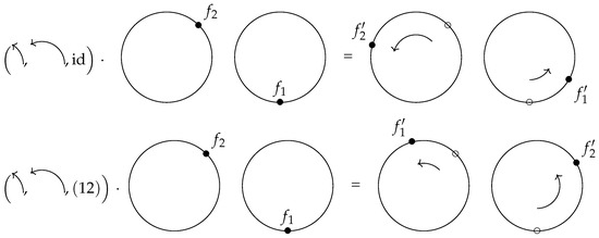
(Wreath product action on frames of two disjoint circles). We again consider $G=U\left(1\right)$ and $F=S^1\bigsqcup S^1$. Again, $S^1$ does not carry any special points, whereas $U\left(1\right)$ does have one in its neutral element. To emphasize this in the picture, we visualize elements of $S^1$ as points on a circle, but elements of $U\left(1\right)$ we visualize as rotation arrows. The action first relabels the basis elements, and then acts with the groups elements; see Figure 7 for an example.

Figure 7. Illustration of how the wreath product acts on a tuple of points; here, in the case of F, the $U\left(1\right)$-set $S^1\bigsqcup S^1$. First, the labels are exchanged according to the permutation, and then the group elements act according to this new labeling.

Let us briefly review some basic properties on this wreath product. For $G={\mathbb{F}}^{\times }$, i.e., the unit group of a field $\mathbb{F}$, and $X=I_n$, the wreath product is faithfully represented by $n\times n$ generalized permutation matrices. These are the matrices in $GL(n,\mathbb{F})$ having only a single non-zero entry in each row and column. An explicit representation is $(\tilde{g},\sigma )\mapsto \mathrm{diag}(g_1,\dots ,g_n)P_{\sigma }$, where $P_{\sigma }$ is a standard permutation matrix. If G is a topological/Lie group, then $G\wr X$ is as well via the semi-direct product realization. The connected subgroup of $G\wr X$ is that of $G^X$. Hence, in case G is a Lie group with algebra $\mathfrak{g}$, the algebra of $G\wr X$ is ${\mathfrak{g}}^X$, which we view as the space of functions $X\to \mathfrak{g}$. It follows that $dim(G\wr X)=dim\left(G\right)\left|X\right|$, so for infinite X and non-discrete G, one formally obtains an infinite-dimensional object. However, because $G\wr X$ locally looks like separate copies of G and we assume G to be finite dimensional, we do not dwell on this.

Having introduced the wreath product, we may now define how it acts on $F^X$. We simply combine the previous actions on $F^X$ by stating that a pair $(\tilde{g},\sigma )\in G^X\times Sym\left(X\right)$ acts by first acting with $\sigma$ and then acting by $\tilde{g}$. When thinking of the wreath product in terms of generalized permutation matrices, this action resembles matrix–vector multiplication by viewing $\tilde{f}$ as a column vector.

Proposition 6.

The map

$$\begin{array}{cc}\hfill G\wr X\times F^X& \to F^X\hfill \\ \hfill ((\tilde{g},\sigma ),\tilde{f})& \mapsto \tilde{g}(\tilde{f}\circ {\sigma }^{-1})\hfill \end{array}$$

(31)

defines a $G\wr X$-action on $F^X$. Moreover, $Fr\left(F\right)$ is an invariant subset, even a $G\wr X$-torsor.

Proof. 

Let us check that the proposed map indeed defines a $G\wr X$-action. Clearly, the identity element of $G\wr X$ fixes any $\tilde{f}$, and for the homomorphism property, one checks

$$(\tilde{g},\sigma )\left[({\tilde{g}}^{\prime },{\sigma }^{\prime })\tilde{f}\right]=(\tilde{g},\sigma )\left[{\tilde{g}}^{\prime }\left(\tilde{f}{\sigma }^{\prime -1}\right)\right]=\tilde{g}\left({\tilde{g}}^{\prime }{\sigma }^{-1}\right)\left(\tilde{f}{\sigma }^{\prime -1}{\sigma }^{-1}\right)=[\tilde{g}\left({\tilde{g}}^{\prime }{\sigma }^{-1}\right),\sigma {\sigma }^{\prime })]\tilde{f}.$$

(32)

So, indeed $(\tilde{g},\sigma )\left[({\tilde{g}}^{\prime },{\sigma }^{\prime })\tilde{f}\right]=\left[(\tilde{g},\sigma )({\tilde{g}}^{\prime },{\sigma }^{\prime })\right]\tilde{f}$; hence, the above map defines a $G\wr X$-action.

To check the restriction to $Fr\left(F\right)$, we check the criterion of Lemma 7. If $\tilde{f}\in Fr\left(F\right)$, then $q\tilde{f}$ is invertible and hence

$$q\left((\tilde{g},\sigma )\tilde{f}\right)=q\left(\tilde{g}\left(\tilde{f}{\sigma }^{-1}\right)\right)=q\tilde{f}{\sigma }^{-1}$$

(33)

is invertible. Hence, $(\tilde{g},\sigma )\tilde{f}\in Fr\left(F\right)$, implying that the action restricts to $Fr\left(F\right)$. Concerning the last claim, pick two frames $\tilde{f}$ and ${\tilde{f}}^{\prime }$. Then, $q\tilde{f}$ and $q{\tilde{f}}^{\prime }$ are invertible; hence, one obtains a permutation $\sigma ={\left(q{\tilde{f}}^{\prime }\right)}^{-1}q\tilde{f}$. It follows that $\sigma ·\tilde{f}$ and ${\tilde{f}}^{\prime }$ have the same underlying permutation, as $q(\sigma ·\tilde{f})=q\tilde{f}{\sigma }^{-1}=q\tilde{f}{\left(q\tilde{f}\right)}^{-1}q{\tilde{f}}^{\prime }=q{\tilde{f}}^{\prime }$. Hence, for each $x\in X$, the elements $(\sigma ·\tilde{f})\left(x\right)$ and ${\tilde{f}}^{\prime }\left(x\right)$ lie in the same G-orbit, and as F is free, they are related by a unique group element $\tilde{g}\left(x\right)$. This means that $\sigma ·\tilde{f}$ and ${\tilde{f}}^{\prime }$ are related by a unique element of $G^X$. Hence, any two frames can be related by a unique element of $G\wr X$, i.e., the action is free and transitive. □

We wish to make a technical remark on the choice of the group. Observe that the symmetry group of the basis $Fr\left(F\right)$ can also be argued to be $Aut\left(F\right)$. Indeed, given any two bases $\tilde{f}$ and ${\tilde{f}}^{\prime }$, the map ${\varphi }_{\tilde{f}}^{\prime }{\varphi }_{\tilde{f}}^{-1}$ is an element of $Aut\left(F\right)$, even the unique element which brings $\tilde{f}$ to ${\tilde{f}}^{\prime }$. It follows that this action on $Fr\left(F\right)$ is also free and transitive. Hence, one could pick either $G\wr X$ or $Aut\left(F\right)$ as the symmetry group of F. However, there is a subtle yet significant difference between the two.

Let us illustrate this difference in the more familiar setting of a real vector space V of dimension n. Clearly, $Fr\left(V\right)$ has a natural action by $GL(n,\mathbb{R})$; a matrix $A=\left(A_{ij}\right)\in GL(n,\mathbb{R})$ acts on a basis as

$$A·(v_1,\dots ,v_n)=(A_{1i}{v}_i,\dots ,A_{ni}{v}_i),$$

(34)

where repeated indices are summed over. However, one may argue that the symmetry group of $Fr\left(V\right)$ is $GL\left(V\right)$, as this is the automorphism group of V. The action of $\varphi \in GL\left(V\right)$ on a basis is

$$\varphi ·(v_1,\dots ,v_n)=(\varphi \left(v_1\right),\dots ,\varphi \left(v_n\right)).$$

(35)

This is again free and transitive, similar to the $GL(n,\mathbb{R})$-action. Of course, $GL\left(V\right)$ is isomorphic to $GL(n,\mathbb{R})$. However, let us try to use these actions to define new actions but now on $Fr\left(V^{\prime }\right)$, where $V^{\prime }$ is another real vector space of dimension n. We see that the $GL(n,\mathbb{R})$-action can be copied verbatim; A acting on a basis $(v_1^{\prime },\dots ,v_n^{\prime })$ of $V^{\prime }$ is simply $(A_{1i}{v}_i^{\prime },\dots ,A_{ni}{v}_i^{\prime })$. This is not so for the $GL\left(V\right)$-action; $\varphi \in GL\left(V\right)$ takes elements of V and not of $V^{\prime }$. Even in the case $V={\mathbb{R}}^n$, this subtle issue arises. In this notation, under the $GL(n,\mathbb{R})$-action, every vector in the new basis depends on all the old ones, whereas under the $GL\left({\mathbb{R}}^n\right)$-action, every new vector depends only on the previous one. In particular, if one perturbs only one of the basis vectors, then this may change all vectors under the $GL(n,\mathbb{R})$-action but only one under the $GL\left({\mathbb{R}}^n\right)$-action. As a final remark, note that vector bundles describe a smooth family of vector spaces. When defining the frame bundle of a vector bundle, it is this crucial that a global $GL(n,\mathbb{R})$-action can be defined, despite the fact that every fiber involves another vector space.

For G-sets, we find a similar argument; instead of using $Aut\left(F\right)$, we will use $G\wr X$. This will be important when we discuss bundles involving G-spaces later on. A more detailed exploration of $Aut\left(F\right)$ and how it is isomorphic to the wreath product $G\wr X$ is given in Appendix A.

4.4. Representing Equivariant Maps Using Matrices

Having seen the relevant group for G-bases, namely, the wreath product, we can continue with how to use G-bases for representing equivariant maps. The analogy with vector spaces is again a good lead. There, if $(v_1,v_2)$ is a basis of the given vector space, one can express the linear map A using a matrix by calculating $A{v}_1$ and $A{v}_2$ and relating these back to $v_1$ and $v_2$. The matrix is then the array of all the coefficients, which are unique but depend on the choice of basis. To list the procedure explicitly,

$$\left(\begin{array}{c}A{v}_1\\ A{v}_2\end{array}\right)=\left(\begin{array}{c}{A}_{11}{v}_1+A_{12}{v}_2\\ A_{21}{v}_1+A_{22}{v}_2\end{array}\right)=\left(\begin{array}{cc}{A}_{11}& A_{12}\\ A_{21}& A_{22}\end{array}\right)\left(\begin{array}{c}{v}_1\\ v_2\end{array}\right).$$

(36)

For semi-torsors, we have essentially the same equation. If $(f_1,f_2)$ is a basis of the given semi-torsor, one can express the G-equivariant map $\alpha$ using a matrix by calculating $\alpha \left(f_1\right)$ and $\alpha \left(f_2\right)$ and listing how these relate to $f_1$ and $f_2$. Let us first give an example, and then state the general argument.

Example 9.

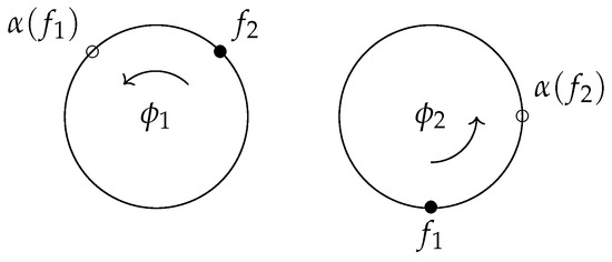
Let us take a situation like the parallel transport map on the double torus. That is, we consider the $U\left(1\right)$-semi-torsor $S^1\bigsqcup S^1$, and there is an equivariant map α. We pick a basis $(f_1,f_2)$ of $S^1\bigsqcup S^1$, and calculate $\alpha \left(f_1\right)$ and $\alpha \left(f_2\right)$, leading to a situation as in Figure 8. In this case, we find

$$\left(\begin{array}{c}\alpha \left(f_1\right)\\ \alpha \left(f_2\right)\end{array}\right)=\left(\begin{array}{c}{e}^{i{\varphi }_1}{f}_2\\ e^{i{\varphi }_2}{f}_1\end{array}\right)=\left(\begin{array}{cc}0& e^{i{\varphi }_1}\\ e^{i{\varphi }_2}& 0\end{array}\right)\left(\begin{array}{c}{f}_1\\ f_2\end{array}\right).$$

(37)

Figure 8. Using a frame to describe an equivariant map, such as parallel transport. One expresses $\alpha \left(f_1\right)$ and $\alpha \left(f_2\right)$ using the basis $(f_1,f_2)$ and so finds the (matrix) coefficients.

The zeros here just mean that those entries are not needed. This matrix representing α is a generalized permutation matrix; it can be decomposed as

$$\left(\begin{array}{cc}0& e^{i{\varphi }_1}\\ e^{i{\varphi }_2}& 0\end{array}\right)=\left(\begin{array}{cc}{e}^{i{\varphi }_1}& 0\\ 0& e^{i{\varphi }_2}\end{array}\right)\left(\begin{array}{cc}0& 1\\ 1& 0\end{array}\right)$$

(38)

that is, as the product of a diagonal and a permutation matrix. The diagonal matrix lists all the needed group translations, while the permutation matrix describes how the orbits are exchanged. The exact elements again depend on the chosen frame $(f_1,f_2)$.

This extraction of the matrix works for arbitrary bases of a semi-torsor, even in the case when $\alpha :F\to F^{\prime }$ relates semi-torsors with a different amount of orbits. To describe this, let $(f_1,\dots ,f_n)$ be a basis of F, and $(f_1^{\prime },\dots ,f_m^{\prime })$ a basis of $F^{\prime }$. The main point is that $\alpha \left(f_i\right)$ will always be in the orbit of a unique $f_j^{\prime }$, and these elements will then differ by a unique element $g_i$, i.e., $\alpha \left(f_i\right)=g_i{f}_j^{\prime }$. Defining the matrix A, with elements in G, by

$$A_{ji}=\left\{\begin{array}{cc}{g}_i\hfill & \mathrm{if}\alpha \left(f_i\right)=g_i{f}_j^{\prime }\hfill \\ 0\hfill & \mathrm{else}\hfill \end{array}\right.$$

(39)

then generalizes the previous recipe. At this point, A is just an array of elements in G. In a special case, namely, when G is commutative, one recovers the property that matrix multiplication corresponds to the composition of maps.

Lemma 8.

Let $\alpha :F\to F^{\prime }$ and $\beta :F^{\prime }\to F^{″}$ be G-equivariant maps of G-semi-torsors, and let $\tilde{f}$ be a frame of F and ${\tilde{f}}^{″}$ a frame of $F^{″}$. Pick a basis ${\tilde{f}}^{\prime }$ of $F^{\prime }$ so that α and β are represented by matrices A and B with respect to the appropriate bases. If G is commutative, then the matrix representing $\beta \circ \alpha$ equals the matrix product $BA$.

Proof. 

Say $\beta \left({\tilde{f}}_i^{\prime }\right)=g_i^{\prime }{\tilde{f}}_{{\sigma }^{\prime }\left(i\right)}^{″}$. The matrix $\widehat{\beta \alpha }$ has at position $({\sigma }^{\prime }\sigma \left(i\right),i)$ the element $g_i{g}_{\sigma \left(i\right)}^{\prime }$ as

$$\beta \left(\alpha \left(f_i\right)\right)=\beta \left(g_i{f}_{\sigma \left(i\right)}^{\prime }\right)=g_i\beta \left(f_{\sigma \left(i\right)}^{\prime }\right)=g_i{g}_{\sigma \left(i\right)}^{\prime }{f}_{{\sigma }^{\prime }\sigma \left(i\right)}^{″}.$$

(40)

If G is commutative, this equals $g_{\sigma \left(i\right)}^{\prime }{g}_i$. Going over all i, we find the n non-trivial coefficients for $\beta \circ \alpha$, and these coincide with those obtained from the multiplication $BA$. □

For a self-map $\alpha :F\to F$, changing the basis causes the matrix A to change by conjugation. That is, if $\tilde{f}$ is changed to $(\tilde{g},\sigma )·\tilde{f}$, then A is conjugated by the generalized permutation matrix representing $(\tilde{g},\sigma )$. A logical question is then what properties of A are invariant under the choice of basis. Similar to linear algebra, this can be performed by investigating the invariant subspaces of $\alpha$—please remember that $\alpha$ contains the actual information, of which A gives some non-unique representation. This leads to equivalents of the Jordan normal form and eigenvalues for these matrices as we describe in the following.

Proposition 7.

Let F be a G-semi-torsor and $\alpha :F\to F$ an automorphism. Then, we have the following:

• $F={\bigsqcup }_{i\in I}{F}_i$, for some index set I, decomposes F into minimal α-invariant subspaces, i.e., $\alpha \left(F_i\right)=F_i$ for all i.
• If G is commutative and a particular $F_i$ consists of $k<\infty$ orbits, then ${\left(\alpha {|}_{F_i}\right)}^k$ equals translation by an element ${\Lambda }_i$ of G.
• By picking the appropriate basis of F, the matrix A can be written in block diagonal form. A block represents a restriction ${\alpha |}_{F_i}$, with size given by the number of orbits k, and one may choose one of the following normal forms for it. The first of these is, with $e\in G$ the identity,

  $$\left(\begin{array}{ccccc}& & & & {\Lambda }_i\\ e& 0& \dots & 0& \\ 0& e& \dots & 0& \\ & & \ddots & & & \\ 0& 0& \dots & e& \end{array}\right)$$

  (41)

  and a second form is, given any ${\lambda }_i\in G$ such that ${\lambda }_i^k={\Lambda }_i$,

  $$\left(\begin{array}{ccccc}& & & & {\lambda }_i\\ {\lambda }_i& 0& \dots & 0& \\ 0& {\lambda }_i& \dots & 0& \\ & & \ddots & & & \\ 0& 0& \dots & {\lambda }_i& \end{array}\right).$$

  (42)

Proof. 

Clearly, the index set I is obtained by taking the original orbit space X and identifying orbits that are mapped into one another by $\alpha$. We focus on a particular minimal subspace $F_i$. If $F_i$ consists of k orbits, then by minimality, ${\left(\alpha {|}_{F_i}\right)}^k$ preserves the orbits in $F_i$. Picking $f\in F_i$, we find ${\alpha }^k\left(f\right)=g\left(f\right)f$ for some $g\left(f\right)\in G$. To inspect how this depends on f, let us write another element in the orbit as $hf$ with $h\in G$. If G is commutative, one finds both

$${\alpha }^k\left(hf\right)=h{\alpha }^k\left(f\right)=hg\left(f\right)f\mathrm{and}{\alpha }^k\left(hf\right)=g\left(hf\right)hf=hg\left(hf\right)f$$

(43)

and as F is free, this yields $hg\left(f\right)=hg\left(hf\right)$, and applying $h^{-1}$ yields $g\left(hf\right)=g\left(f\right)$. That is, $g\left(f\right)$ is constant on the orbit through f. It is even constant on the invariant subspace $F_i$; as equivariance yields ${\alpha }^k\left(\alpha \left(f\right)\right)=g\left(f\right)\alpha \left(f\right)$, we see that $\alpha \left(f\right)$ in the next orbit is scaled by the same group element. It follows that $g\left(f\right)$ is constant on the subspace $F_i$, and we write this group element as ${\Lambda }_i$. The first normal form is obtained by picking a basis as follows. One picks any $f_1\in F_i$, and then inductively sets $f_{j+1}=\alpha \left(f_j\right)$. It then follows that all group elements are the identity, except when dealing with $\alpha \left(f_k\right)$, which gives $\alpha \left(f_k\right)={\alpha }^k\left(f_1\right)={\Lambda }_i{f}_1$ and so proves the first normal form. The second normal form is obtained by the rule $f_{j+1}={\lambda }_i^{-1}\alpha \left(f_j\right)$. We only need to check that this yields $\alpha \left(f_k\right)={\lambda }_i{f}_1$, which follows from

$$\alpha \left(f_k\right)={\lambda }_i^{-1}{\alpha }^2\left(f_{k-1}\right)=\cdots ={\lambda }_i^{-(k-1)}{\alpha }^k\left(f_1\right)={\lambda }_i^{-(k-1)}{\Lambda }_i{f}_1={\lambda }_i{f}_1.$$

(44)

□

Example 10.

In the situation of the previous example, $F=S^1\bigsqcup S^1$ is already a minimal invariant subspace, as both orbits are mapped to one another. For the characteristic group element, we consider ${\alpha }^2$, as there are two orbits, and we see that ${\alpha }^2\left(f\right)=e^{i({\varphi }_1+{\varphi }_2)}f$. The invariant group element is thus $\Lambda =e^{i({\varphi }_1+{\varphi }_2)}f$, and is thus given by the sum ${\varphi }_1+{\varphi }_2$ of the angles, which is the ‘return angle’.

The normal forms offer us two standard ways to distribute this total angle over the steps. The first is to perform the entire angle in one step, and the second is to distribute it evenly over the steps. This is illustrated in Figure 9 below. In the picture, α lays the right circle over the left one with a rotation of $+225$ degrees, and the left circle over the right one with $-45$ degrees. The return angle is thus 180 degrees. The first option picks a frame where the entire angle occurs when evaluating $f_2$. The second option picks a frame where this angle is distributed evenly over $f_1$ and $f_2$. We can choose any of the roots of the 180 degree rotation, so either $+90$ or $-90$ degrees each time. The matrices are thus

$$\left(\begin{array}{cc}0& -1\\ 1& 0\end{array}\right)\mathrm{and}\left(\begin{array}{cc}0& \pm i\\ \pm i& 0\end{array}\right).$$

(45)

Figure 9. Bases for the two normal forms. Left: first normal form with the entire angle ${\varphi }_t={\varphi }_1+{\varphi }_2$ in the last step. As $f_2:=\alpha \left(f_1\right)$, the rotation there vanishes. Right: second normal form, with the angle evenly distributed over the steps.

In Figure 9, we chose the + option in the second normal form.

4.5. Functorial Property

The previous material indicates that a G-semi-torsor F can be mapped to the $G\wr (F/G)$-torsor $Fr\left(F\right)$. Such a statement hints at a functorial property, which brings us to the question which equivariant maps $\alpha :F_1\to F_2$ will induce a map on frames $Fr\left(F_1\right)\to Fr\left(F_2\right)$ in the canonical way $\tilde{f}\mapsto \alpha \circ \tilde{f}$. As we assume that $F_1$ and $F_2$ are free, this can be answered by looking at orbits only. We first show that $\alpha$ induces a unique map on the quotients, and that the invertibility of this map is equivalent to the posed question.

Lemma 9.

Let $F_i$ be $G_i$-semi-torsors with orbits spaces $X_i=F_i/G_i$ for $i=1,2$. Let $\alpha :F_1\to F_2$ be a ξ-equivariant map. Then, α descends to a unique map on orbits $\alpha /:F_1/G_1\to F_2/G_2$. That is, there is a unique arrow such that the following diagram commutes:

(46)

Moreover, an equivariant map $\alpha :F_1\to F_2$ lifts to a map $\alpha !:Fr\left(F_1\right)\to Fr\left(F_2\right)$ if and only if $\alpha /:X_1\to X_2$ is a bijection, i.e., if α is a bijection on orbit level. In this case, and after identifying $X_1$ and $X_2$ with X for simplicity, $\alpha !$ is equivariant with respect to the group map $\xi !=({\xi }^X,{\mathrm{id}}_{Sym\left(X\right)}):G_1\wr X\to G_2\wr X$.

Proof. 

By equivariance, $\alpha$ maps a $G_1$-orbit in $F_1$ inside a single $G_2$-orbit in $F_2$. That is, the map $q_2\circ \alpha$ is $G_1$-invariant. Hence, $\alpha /$ exists as a function. More generally, as the $X_i$ are discrete, this map is also continuous. Let us thus consider the induced maps on the bases. The statement is trivial in case $X_1$ and $X_2$ are not bijective; then, bases of $F_1$ and $F_2$ have unequal cardinality, but also $\alpha /$ cannot be a bijection. Hence, we treat the case $X_1\cong X_2\cong X$. In this case, there is a well-defined function ${\alpha }^X:F_1^X\to F_2^X$ given by $\tilde{f}\mapsto \alpha \circ \tilde{f}$. To check that $\alpha \circ \tilde{f}$ is a basis of $F_2$ whenever $\tilde{f}$ is a basis of $F_1$, we use the criterion in Lemma 7. This concerns the invertibility of

$$q_2\circ \alpha \circ \tilde{f}=\alpha /\circ q_1\circ \tilde{f}.$$

(47)

From this equation, it follows that for $q_2\circ \alpha \circ \tilde{f}$ to be invertible whenever $q_1\circ \tilde{f}$ is, it is both necessary and sufficient that $\alpha /$ is a bijection. Concerning equivariance, note that ${\alpha }^X$ is ${\xi }^X$-equivariant. Moreover, ${\alpha }^X$ is also $Sym\left(X\right)$-equivariant as

$$\sigma \left({\alpha }^X\left(\tilde{f}\right)\right)=\sigma \left(\alpha \tilde{f}\right)=\alpha \tilde{f}{\sigma }^{-1}={\alpha }^X\left(\tilde{f}{\sigma }^{-1}\right)={\alpha }^X\left(\sigma \tilde{f}\right).$$

(48)

That is, ${\alpha }^X$ is equivariant with respect to both ${\xi }^X$ and ${\mathrm{id}}_{Sym\left(X\right)}$, which implies that ${\alpha }^X$ is equivariant with respect to the map $\xi !:G_1\wr X\to G_2\wr X$ given by $({\xi }^X,{\mathrm{id}}_{Sym\left(X\right)})$. As the actions are restricted to the frames, the restriction $\alpha !$ of ${\alpha }^X$ to the frames is again equivariant with respect to $\xi !$. □

The requirement in this result is not automatic; there exist equivariant maps of semi-torsors that are not a bijection on orbit level. A simple example is mapping $G\bigsqcup G$ to G via identity maps. Hence, taking the frame space can only form a functor from semi-torsors to torsors if the maps $\alpha$ between semi-torsors are restricted to those where $\alpha /$ is a bijection. Let us thus define the following categories.

Definition 8.

Define STor to be the category whose objects are semi-torsors and whose maps are equivariant morphisms α so that $\alpha /$ is a bijection. Given a Lie group G, write ${STor}_G$ for the restriction of STor to G-semi-torsors and ${\mathrm{id}}_G$-equivariant morphisms.

By restricting the category of group spaces to torsors, one obtains the category Tor of torsors, and also the category ${Tor}_G$ by requiring the group to be G and morphisms to be ${\mathrm{id}}_G$-equivariant. It is clear that Tor is a full subcategory of STor. Taking the frame space then defines a retraction in the following sense.

Theorem 1.

The assignment

$$\begin{array}{cc}\hfill F& \mapsto Fr\left(F\right)\hfill \\ \hfill \alpha & \mapsto \alpha !,\hfill \end{array}$$

(49)

defines a covariant functor $STor\to Tor$. Moreover, this functor is (essentially) constant on Tor.

Proof. 

Observe that the source is a well-defined category; any identity map trivially satisfies the condition of Lemma 9, and the composition of maps preserves this condition; if $\alpha$ and $\beta$ are composable maps which satisfy that $\alpha /$ and $\beta /$ are bijections, then as $\left(\alpha \beta \right)/=\alpha /\beta /$, also $\alpha \beta$ does. By Proposition 6 and Lemma 9, the assignment is well defined on objects, i.e., maps. Given the explicit form of $\alpha !$ in Lemma 9, it follows that ${\mathrm{id}}_F!={\mathrm{id}}_{Fr\left(F\right)}$ and $\left(\alpha \beta \right)!=\alpha !\beta !$. Hence, the assignment is a functor. As $Fr\left(F\right)$ is a $G\wr X$-torsor and $\alpha !$ is equivariant, this functor takes the image in the category of torsors. If F is already a torsor, then X consists of a single point, and the condition of Lemma 7 is vacuous, so $Fr\left(F\right)=F^X\cong F$. Hence, the functor is (essentially) constant on the torsors. □

If one fixes the structure group G, then one can say more. The image of ${STor}_G$ consists of torsors whose structure groups are of the form $G\wr X$. Given a particular torsor in this image, up to isomorphism, the original semi-torsor can be recovered by taking a quotient. The idea is that a semi-torsor F can be recovered from $Fr\left(F\right)$ by considering all elements that appear in any particular position $x\in X$ in the tuples. This position we may choose ourselves, e.g., we only consider the first position. This is equivalent to quotienting $Fr\left(F\right)$ by the subgroup $G\wr (X-x)$ of all group elements that do not touch position x. This yields a method applicable to any $G\wr X$-torsor, and we obtain an equivalence of categories. In order to show this, it is convenient to first treat the following lemma. This shows that the model $G\wr X$-torsor, being the space $G\wr X$ viewed as a torsor, indeed reduces to $G\times X$, which we expect, as $Fr(G\times X)$ is isomorphic to $G\wr X$ (as torsors). The action we will use can be obtained by viewing elements of $G\wr X$ as generalized permutation matrices, and $(h,x)\in G\times X$ as a column vector consisting of all zeros, except for h at place x.

Lemma 10.

There is an action of $G\wr X$ on $G\times X$ defined by

$$(\tilde{g},\sigma )·(h,x)=(\tilde{g}\left(\sigma \left(x\right)\right)h,\sigma \left(x\right)).$$

(50)

The stabilizer of $(h,x)$ is the subgroup $G\wr (X-x)$. Moreover, the induced map $\frac{G\wr X}{G\wr (X-x)}\to G\times X$, where the quotient is endowed with the G-action on slot x, is an isomorphism in ${STor}_G$.

Proof. 

To check the action property, observe that

$$\begin{array}{cc}\hfill \left[(\tilde{g},\sigma )(\tilde{h},\tau )\right]·(z,x)& =(\tilde{g}\left(\sigma \tau \left(x\right)\right)\tilde{h}\left(\tau \left(x\right)\right)z,\sigma \tau \left(x\right))\hfill \\ \hfill & =(\tilde{g},\sigma )·(\tilde{h}\left(\tau \left(x\right)\right)z,\tau \left(x\right))=(\tilde{g},\sigma )·[(\tilde{h},\tau )·(z,x)].\hfill \end{array}$$

(51)

Furthermore, $(\tilde{g},\sigma )$ lies in the stabilizer of $(h,x)$ if and only if $\sigma \left(x\right)=x$ and $\tilde{g}\left(x\right)=1$. That is, the place indexed by x is not touched. Hence, the stabilizer is canonically identified with $G\wr (X-x)$. Viewing $G\wr X$ as a G-space as indicated, the orbit map $G\wr X\to G\times X$ is G-equivariant, and so the quotient yields an isomorphism of G-semi-torsors. □

An equivalence of categories can now be obtained as follows. To avoid confusion concerning the class of all discrete topological spaces, we restrict to the finite case.

Proposition 8.

For a fixed Lie group G, the frame functor induces an equivalence of categories

$${STor}_G^{<\infty }\to \coprod _{n=1}^{\infty }{Tor}_{G\wr I_n},$$

(52)

where the superscript $<\infty$ indicates the restriction to finite index sets.

Proof. 

Let us show that this restricted functor is both fully faithful and essentially surjective. Given a $G\wr I_n$-torsor T so that T is isomorphic to the space $G\wr I_n$ viewed as torsor, by Lemma 10 one has $Fr\left(T/(G\wr (I_n-1))\right)\cong G\wr I_n\cong T$, and hence the functor is essentially surjective. To show it is fully faithful, let $F,F^{\prime }$ be two G-semi-torsors with equal index set $I_n$. Let $\overline{\alpha }:Fr\left(F\right)\to Fr\left(F^{\prime }\right)$ be any map of $G\wr I_n$-torsors. Pick any frame $\tilde{f}\in Fr\left(F\right)$. Using its image frame $\overline{\alpha }\left(\tilde{f}\right)$, define the map $\alpha :={\varphi }_{\overline{\alpha }\left(\tilde{f}\right)}\circ {\varphi }_{\tilde{f}}^{-1}:F\to F^{\prime }$, which does not depend on our choice of $\tilde{f}$. Clearly, $\alpha$ is the unique morphism $F\to F^{\prime }$ satisfying $Fr\left(\alpha \right)=\overline{\alpha }$. Hence, the functor is also fully faithful, and the equivalence follows. □

5. The Frame Bundle of a Semi-Principal Bundle

In this final section, we introduce the frame bundle of a semi-principal bundle, which again closely resembles the frame bundle of a vector bundle. We have already seen semi-principal parallel transport, and demonstrated how frames can be used to study this. With the frame bundle, frames become an inherent part of the bundle structure itself. As the frame bundle is principal, it thus allows for a conventional way to study parallel transport straightaway. We will first define the frame bundle, then demonstrate its functorial nature, and finish with the passage of a connection on a semi-principal bundle to a connection on the frame bundle.

5.1. The Frame Bundle of a Semi-Principal Bundle

We thus start by defining the frame bundle $Fr\left(B\right)$ of a semi-principal G-bundle $B\to M$ with model fiber F. Let us stay close to the argument we had for $Fr\left(F\right)$, which consist of two steps. First, we showed that $F^X$ has a natural $G\wr X$-action on it, to then view $Fr\left(F\right)$ as a special subspace. We have the same steps here. To start, instead of $F^X$, we first inspect the $G\wr X$-action on the X-fold fiberwise product bundle ${\pi }^{\odot X}:B^{\odot X}\to M$ of B.

Proposition 9.

Given a semi-principal G-bundle $\pi :B\to M$ with index set X, then the fiberwise product bundle $F^X\to B^{\odot X}\to M$ is canonically a $G\wr X$-space bundle.

Proof. 

It is convenient to realize $B^{\odot X}$ as a pull-back of the X-fold direct product bundle

$$\begin{array}{ccccc}\hfill F^X& \to & B^X& \stackrel{{\pi }^X}{\to }& M^X.\hfill \end{array}$$

(53)

As B is a G-space, clearly $B^X$ is a $G\wr X$-space by a similar argument to that we used for $F^X$ in Proposition 6. Likewise, $M^X$ is a $Sym\left(X\right)$-space, and ${\pi }^X$ is equivariant for the canonical group map $G\wr X\to Sym\left(X\right)$. Moreover, ${\pi }^X$ admits $G\wr X$-equivariant local trivializations. Indeed, let ${\varphi :U\times F\to B|}_U$ be a local G-equivariant trivialization of B. This induces the map

$$\begin{array}{cc}\hfill {\varphi }^X:U^X\times F^X& \to B^X{|}_{U^X}\hfill \\ \hfill (u\left(x\right),\tilde{f}\left(x\right))& \mapsto \varphi (u\left(x\right),\tilde{f}\left(x\right)),\hfill \end{array}$$

(54)

which is a local trivialization of $B^X$. It is $G\wr X$-equivariant; the $G^X$-equivariance is by construction, and the $Sym\left(X\right)$-equivariance is immediate, cf. the verification in the proof of Lemma 9.

Let us move to $B^{\odot X}$. Obviously, tuples in $B^X$ may contain elements from different fibers of B, and we obtain the fiberwise product by demanding that they come from a single fiber. This can be expressed geometrically using the constant/diagonal map $c:M\to M^X$ sending $m\in M$ to the constant function $[x\mapsto m]$. This realizes the fiberwise product bundle $B^{\odot X}$ as a pull-back, whose corresponding diagram is

(55)

so that both bundles have model fiber $F^X$. In this way, the topology and manifold structure of $B^{\odot X}$ are clear, and ${\pi }^{\odot X}$ is smooth. Moreover, as the image of c is $Sym\left(X\right)$-invariant, it follows that $B^{\odot X}$ inherits a $G\wr X$-action from $B^X$ that leaves ${\pi }^{\odot X}$ invariant. A local trivialization $\varphi$ of B induces the local trivialization ${\varphi }^{\odot X}$ of $B^{\odot X}$ given by

$$\begin{array}{cc}\hfill {\varphi }^{\odot X}:U\times F^X& \to B^{\odot X}\hfill \\ \hfill (u,\tilde{f}\left(x\right))& \mapsto \varphi (u,\tilde{f}\left(x\right)),\hfill \end{array}$$

(56)

which is $G\wr X$-equivariant. □

We can now view the frame bundle $Fr\left(B\right)$ of B as the subspace of $B^{\odot X}$ where the elements define bases as performed formally in the following definition. Given the previous result, it is only a minor step to prove the bundle property of $Fr\left(B\right)$, which we perform directly afterwards.

Definition 9.

Given a semi-principal G-bundle $\pi :B\to M$, its frame bundle is defined as the bundle

$$Fr\left(B\right)=\left\{\tilde{b}\in B^{\odot X}|\tilde{b}\mathit{is}\mathrm{a}\mathit{basis}\mathit{of}\mathit{the}\mathit{corresponding}\mathit{fiber}\mathit{of}\mathit{B}\right\}.$$

(57)

Theorem 2.

If $\pi :B\to M$ is a semi-principal G-bundle, then its frame bundle $Fr\left(B\right)$ is an open subbundle of $B^{\odot X}$, and forms a principal bundle

$$\begin{array}{ccccc}\hfill G\wr X& \to & Fr\left(B\right)& \to & M.\hfill \end{array}$$

(58)

Proof. 

Given Proposition 9, it suffices to verify that $Fr\left(F\right)$ is locally an open subbundle of $B^{\odot X}$. Let $U\subset M$ be a trivializing open of B, consider the induced local trivialization ${\varphi }^{\odot X}:U\times F^X\to B^{\odot X}{|}_U$. As $Fr\left(F\right)$ is open and closed in $F^X$ by Corollary 2, the map ${\varphi }^{\odot X}$ restricts to a $G\wr X$-equivariant isomorphism from $U\times Fr\left(F\right)$ onto its image. This image is ${Fr\left(B\right)|}_U$, as for each $u\in U$ the map $\varphi$ establishes an isomorphism $F\to B_u$ of G-spaces. Hence, $Fr\left(B\right)$ is an open subbundle of $B^{\odot X}$ with model fiber $Fr\left(F\right)$. As $Fr\left(F\right)$ is a $G\wr X$-torsor by Proposition 6, the bundle is principal. □

We place the following comment concerning the notation $Fr\left(B\right)$. This notation makes explicit reference to the G-manifold B but implicitly uses the bundle map $\pi$ as well. As seen in Example 11 below, different projection maps may lead to different frame bundles, yet the total space of these projection maps is the same G-manifold. We thus write $Fr\left(B\right)$ with the understanding that B is short for the entire bundle structure.

Example 11

(Frame bundle of winding torus). Let us again consider the semi-principal bundles ${\Pi }_k:T^2\to S^1$. The total space is the same for all these bundles, but the frame bundles are different for every k. We already know that the model fiber is ${\bigsqcup }^k{S}^1$, and that $Fr\left({\bigsqcup }^k{S}^1\right)={\bigsqcup }^{k!}{T}^k\cong T^k\times S_k$. These have a different dimension for every k, from which it clearly follows that the frame bundle will be different for each k.

The following question we did not yet answer here: if one wishes to have a well-defined permutation action on the bundle, is it really necessary to leave B behind and move to $Fr\left(B\right)$ instead? In other words, does such an action not already exist on B itself? The need for this change is proven in Appendix B, where we find that one can only stay on B if B is trivial. That is, the local labeling with index set X will in general not suffice in order to define a global permutation action. The solution that $Fr\left(B\right)$ provides for this problem is to use the positions in the frame tuples instead—these positions are defined globally.

5.2. Functoriality of Taking the Frame Bundle

We move on to the functorial nature of the association $B\mapsto Fr\left(B\right)$. In Theorem 1, we proved the functorial nature in the case of semi-torsors, and here we show its extension to semi-principal bundles. Clearly, the objects of the source category are the semi-principal bundles. However, the admissible maps will not be all equivariant bundle maps; inspecting a single fiber brings us back to Lemma 9, which indicates that a map should be a bijection on orbits. This condition readily lifts to the level of bundles, and is a sufficient condition to obtain an induced map on the frame bundles as proven below.

Lemma 11.

Let $\alpha :B_1\to B_2$ be an equivariant bundle map of semi-principal bundles over M, where the map on groups is $\xi :G_1\to G_2$, and $X_1\cong X_2\cong X$. Then, α descends to a fiberwise map on orbits $\alpha /:B_1/G_1\to B_2/G_2$. That is, in the following diagram, the lower arrow exists and is a bundle map.

(59)

Moreover, α induces a map of bundles

$$\begin{array}{cc}\hfill \alpha !:Fr\left(B_1\right)& \to Fr\left(B_2\right)\hfill \\ \hfill \tilde{b}& \mapsto \alpha \circ \tilde{b}\hfill \end{array}$$

(60)

if and only if $\alpha /:B_1/G_1\to B_2/G_2$ is a bundle isomorphism. In this case, $\alpha !$ is equivariant with respect to the map $\xi !=({\xi }^X,{\mathrm{id}}_{Sym\left(X\right)}):G_1\wr X\to G_2\wr X$, so in particular, $\alpha !$ is a map of principal bundles.

Proof. 

As $\alpha$ is equivariant, $\alpha /$ exists as a function, which is fiber-preserving, as the action is so. To prove it is smooth, one can look locally over a trivializing open or use that $Q_1$ is a surjective submersion. Hence, $\alpha /$ is a well-defined bundle map. As $\alpha$ is a bundle map, so is its product ${\alpha }^{\odot X}:B_1^{\odot X}\to B_2^{\odot X}$. The restriction of ${\alpha }^{\odot X}$ is also a bundle map, as $Fr\left(B_1\right)$ is an open subbundle of $B_1^{\odot X}$ by Theorem 2. This restriction takes the image in $Fr\left(B_2\right)$ if and only if $\forall m\in M$ the map ${\alpha }_m:{\left(B_1\right)}_m\to {\left(B_2\right)}_m$ maps bases to bases. By Lemma 9, this is if and only if $\alpha {/}_m:{(B_1/G_1)}_m\to {(B_2/G_2)}_m$ is a bijection for all m. However, as $\alpha /$ is a bundle map, this is equivalent to $\alpha /$ being an isomorphism. The equivariance of $\alpha$ readily follows; a similar derivation as in Lemma 9 applies. Hence, ${\alpha }^{\odot X}$ restricts to the map $\alpha !:Fr\left(B_1\right)\to Fr\left(B_2\right)$ if and only if $\alpha /$ is a bundle isomorphism, in which case $\alpha !$ is a map of principal bundles. □

This result tells us that the frame functor is not applicable to the full subcategory of group-manifold bundles obtained by restricting the fibers to semi-torsors but retaining all possible maps of group-manifold bundles. To obtain a genuine frame functor, we must restrict the maps $\alpha$ to those which satisfy that $\alpha /$ is a bundle isomorphism. Similar to the semi-torsor case in Theorem 1, this will yield a subcategory; ${\mathrm{id}}_B/={\mathrm{id}}_{B/G}$ is always an isomorphism, and a composition of admissible maps is again admissible as $\left(\alpha \beta \right)/=\alpha /\beta /$. Because of its interest in the frame bundle construction, we wish to list this category in a definition.

Definition 10.

The category of semi-principal bundles over a base M, denoted by $SPrin\left(M\right)$, is defined to have as objects the semi-principal bundles over M and as morphisms all equivariant bundles maps α such that $\alpha /$ is an isomorphism. Given a Lie group G, write ${SPrin}_G\left(M\right)$ for the restriction of $SPrin\left(M\right)$ to semi-principal G-bundles and ${\mathrm{id}}_G$-equivariant maps.

Clearly, as we deliberately discard some maps by the orbit condition, $SPrin\left(M\right)$ is a subcategory but not a full subcategory of the group-manifold bundles over M. On the other hand, the principal bundles and their morphisms are still contained in the semi-principal bundles. Let us write $Prin\left(M\right)$ for the category of principal bundles, and ${Prin}_G\left(M\right)$ for the restriction to principal G-bundles and ${\mathrm{id}}_G$-equivariant maps with G as a Lie group. We then find that $SPrin\left(M\right)$ can be seen as a specific extension of $Prin\left(M\right)$.

Lemma 12.

The category $Prin\left(M\right)$ is a full subcategory of $SPrin\left(M\right)$. That is, all principal bundles are semi-principal and ${Hom}_{Prin\left(M\right)}(P,P^{\prime })={Hom}_{SPrin\left(M\right)}(P,P^{\prime })$ whenever P and $P^{\prime }$ are principal bundles over M.

Proof. 

All principal bundles are semi-principal bundles, as any torsor is a semi-torsor. Pick a principal G-bundle P and a principal $G^{\prime }$-bundle $P^{\prime }$ over M, and consider an equivariant bundle map $\alpha :P\to P^{\prime }$. As $P/G\cong M$ and $P^{\prime }/G^{\prime }\cong M$ and $\alpha /$ preserves fibers, one has $\alpha /={\mathrm{id}}_M$ up to an isomorphism. That is, the condition that $\alpha /$ is an isomorphism is automatically satisfied. As this is the only axiom that distinguishes between morphisms in $Prin\left(M\right)$ and $SPrin\left(M\right)$, it follows that ${Hom}_{Prin\left(M\right)}(P,P^{\prime })={Hom}_{SPrin\left(M\right)}(P,P^{\prime })$. □

Back to the frame bundles, one may observe that taking the frame bundle maps $SPrin\left(M\right)$ to its full subcategory $Prin\left(M\right)$. This association is functorial, and can be interpreted as a kind of retract. The formal statement is the following theorem, which is the bundle equivalent of Theorem 1.

Theorem 3.

The assignment

$$\begin{array}{cc}\hfill B& \mapsto Fr\left(B\right)\hfill \\ \hfill \alpha & \mapsto \alpha !\hfill \end{array}$$

(61)

defines a covariant functor $SPrin\left(M\right)\to Prin\left(M\right)$. Moreover, this functor is (essentially) constant on $Prin\left(M\right)$.

Proof. 

By Theorem 2, this functor is well defined on the objects, and by Lemma 11, it is also well defined concerning morphisms. It is easily seen that identity maps and compositions are preserved; hence, the map is a (covariant) functor. Also, if B is a principal bundle, i.e., X is a point, then the basis condition is vacuous and $Fr\left(B\right)=B^X\cong B$. □

Example 12.

An remarkable application of this result is obtained for the quotient map $Q:B\to B/G$. Indeed, this is a morphism in $SPrin\left(M\right)$, where we view $B/G$ as an semi-principal bundle with a trivial structure group. The corresponding bundle map diagram is

(62)

with model fibers indicated. Applying the functor results in the bundle map diagram

(63)

where each arrow is a principal bundle with the indicated structure group.

As with the semi-torsors, also the frame bundle functor induces an equivalence of categories if one fixes the structure group G.

Proposition 10.

For a fixed Lie group G and base manifold M, the frame bundle functor induces an equivalence of categories

$${SPrin}_G^{<\infty }\left(M\right)\to \coprod _{n=1}^{\infty }{Prin}_{G\wr I_n}\left(M\right),$$

(64)

where the superscript $<\infty$ indicates the restriction to finite index sets.

Proof. 

This follows Proposition 8 on semi-torsors; quotienting by $G\wr (I_n-1)$ for each n individually yields again an inverse functor as can be verified using local triviality. □

We finish this exploration of the category $SPrin\left(M\right)$ with the following results on its morphisms.

Lemma 13.

Let $\alpha :B_1\to B_2$ be a morphism in $SPrin\left(M\right)$, equivariant with respect to a group map $\xi :G_1\to G_2$. Then, α can be expressed locally as

$$\rho =({\mathrm{id}}_U,\xi ,{\mathrm{id}}_X):U\times G_1\times X\to U\times G_2\times X$$

(65)

where $U\subset M$ is a trivializing open of both $B_1$ and $B_2$.

Proof. 

For $i=1,2$, let ${\varphi }_i:U_i\times G_i\times X_i\to B_i{|}_{U_i}$ be local trivializations of $B_i$, where $U=U_1\cap U_2$ is non-empty. As $\alpha /$ is an isomorphism, it follows that $X_1\cong X_2$; hence, we call them both X. Restricting the ${\varphi }_i$ to U and identifying $X_i\cong X$, one has the map $\rho ={\varphi }_2^{-1}\alpha {\varphi }_1$. This is a bundle map; hence, the ${\mathrm{id}}_U$ follows. It is also equivariant; hence, a $G_1$-orbit $\left\{u\right\}\times G_1\times \left\{x\right\}$ is mapped inside the $G_2$-orbit $\left\{u\right\}\times G_2\times \left\{x^{\prime }\right\}$. The induced map $x\mapsto x^{\prime }$ on orbits is a bijection by assumption; hence, by identifying $X_2$ with X differently if needed, one may assume $x^{\prime }=x$ for all $x\in X$, which proves the ${\mathrm{id}}_X$ part. The middle map thus remains. Here, note that equivariance reads $\rho (u,g_1,x)=\xi \left(g_1\right)·\rho (u,e_1,x)$ such that $\rho$ is fixed by the points $\rho (u,e_1,x)=(u,g_2(u,x),x)$. This defines a smooth function $g_2(u,x)$, which can be translated to be constant $e_2$ by absorbing it in the $G_2$-part of ${\varphi }_2$ (which does not interfere with the choice for X earlier). However, then, $\rho (u,g_1,x)=\xi \left(g_1\right)·\rho (u,e_1,x)=\xi \left(g_1\right)·(u,e_2,x)=(u,\xi \left(g_1\right),x)$, meaning $\rho$ equals the proposed map. □

Corollary 3.

The map α is injective/surjective if and only if ξ is. Moreover, in case it is surjective, α defines a principal $ker\left(\xi \right)$-bundle.

Proof. 

Let us use the map $\rho$ again. As $\xi$ and $\rho$ only differ by identity maps, $\rho$ is injective/surjective if and only if $\xi$ is. Hence, $\alpha$ is injective/surjective if and only if $\xi$ is. Finally, as $ker\left(\xi \right)$ is a closed normal subgroup of $G_1$, if $\xi$ is surjective, there is the principal bundle $ker\left(\xi \right)\to G_1\to G_2$. Hence, $\xi$ locally looks like ${pr}_V:V\times ker\left(\xi \right)\to V$, where V is a trivializing open in $G_2$. Hence, $\rho$ can be restricted to the map ${\rho }^{\prime }=({\mathrm{id}}_U,{pr}_V,{\mathrm{id}}_X):U\times (V\times ker\left(\xi \right))\times X\to U\times V\times X$, which is clearly $ker\left(\xi \right)$-invariant. As any point in $B_2$ has a neighborhood of the latter form, it follows that $\alpha$ defines a principal $ker\left(\xi \right)$-bundle whenever it is surjective. □

This latter result is the remarkable observation that maps of semi-principal bundles may themselves be principal bundles. We observe that the quotient map $Q:B\to B/G$ provides an example.

5.3. Connection on the Frame Bundle

Let us finish with the connection that the frame bundle inherits from the semi-principal bundle. That is, we need to check how a G-connection on B carries over to a $G\wr X$-connection on $Fr\left(B\right)$. The procedure is straightforward, as $Fr\left(B\right)$ is a submanifold of $B^{\odot X}$. Namely, the latter has a canonically induced connection by stating that a curve

$$\tilde{\Gamma }\left(t\right)={\left({\Gamma }_x\left(t\right)\right)}_{x\in X}$$

(66)

in $B^{\odot X}$ is horizontal if and only if the curves ${\Gamma }_x$ in B are horizontal for all $x\in X$. Equivalently, in the 1-form formalism, the bundle $B^{\odot X}$ is naturally endowed with the $G^X$-connection 1-form ${\omega }^{\odot X}\in {\Omega }^1(B^{\odot X},{\mathfrak{g}}^X)$ defined by

$${\left({\omega }^{\odot X}\right)}_{\tilde{b}}:={\left({\omega }_{b_x}\right)}_{x\in X}=\prod _{x\in X}{\omega }_{b_x}.$$

(67)

We note that this formally leads to infinite dimensional groups and algebras in case X is infinite, but as seen in the curve picture, the connection is nevertheless well defined. A connection $\omega !$ on $Fr\left(B\right)$ is obtained by restriction of ${\omega }^{\odot X}$ to $Fr\left(B\right)$, i.e., one takes the pull-back of ${\omega }^{\odot X}$ along the inclusion $i:Fr\left(B\right)\to B^{\odot X}$. This induced 1-form is indeed a $G\wr X$-connection. A proof of this requires knowledge of the adjoint representation of $G\wr X$; hence, we inspect this first.

Lemma 14.

The adjoint representation $Ad:G\wr X\to GL\left({\mathfrak{g}}^X\right)$ is given by the rules

$$\begin{array}{cc}\hfill {Ad}_{\tilde{g}}& =\prod _{x\in X}{Ad}_{\tilde{g}\left(x\right)}\hfill \\ \hfill {Ad}_{\sigma }& =[\tilde{Y}\mapsto \tilde{Y}{\sigma }^{-1}].\hfill \end{array}$$

(68)

Proof. 

As $(\tilde{g},\sigma )=(\tilde{g},{\mathrm{id}}_X)(\tilde{e},\sigma )$, it suffices to compute the two listed maps. The relevant conjugation maps are

$$\begin{array}{cc}\hfill C_{\tilde{g}}(\tilde{h},\tau )& =(C_{\tilde{g}}\left(\tilde{h}\right),\tau )=(C_{\tilde{g}\left(x\right)}{\left(\tilde{h}\left(x\right)\right)}_{x\in X},\tau )\hfill \\ \hfill C_{\sigma }(\tilde{h},\tau )& =(\tilde{h}{\sigma }^{-1},C_{\sigma }\left(\tau \right)).\hfill \end{array}$$

(69)

The first one recalls that the Ad of $G^X$ is X copies of the Ad of G. The second immediately shows that derivatives follow the same permutation as the tuple. □

Proposition 11.

Let B be a semi-principal G-bundle with G-connection ω. The 1-form

$$\omega !:=i^{\ast }{\omega }^{\odot X}\in {\Omega }^1(Fr\left(B\right),{\mathfrak{g}}^X)$$

(70)

is a $G\wr X$-connection on $Fr\left(B\right)$. In particular, $\omega !$ is a principal connection.

Proof. 

To start, $\omega !$ indeed takes values in the algebra ${\mathfrak{g}}^X$, which is the algebra of $G\wr X$. The condition that $\omega !$ is a left-inverse for the infinitesimal action on $Fr\left(B\right)$ is satisfied, as it is the case per copy, i.e., for each $x\in X$ independently. To check the equivariance of $\omega$, let us consider the $G^X$- and $Sym\left(X\right)$-actions separately. The $G^X$-action can again be inspected per $x\in X$, and reduces to the equivariance of $\omega$. Concerning the permutations, fix $\sigma \in Sym\left(X\right)$. Then, ${\left(L_{\sigma }\right)}^{\ast }\omega !={\prod }_{x\in X}{\omega }_{{\sigma }^{-1}\left(x\right)}={Ad}_{\sigma }(\omega !)$. Hence, $\omega !$ is a $G\wr X$-connection. □

This statement is a hint that the frame bundle functor extends to bundles with connection, which indeed holds according to the upcoming theorem. The intuition is that the connection information on B and $Fr\left(B\right)$ is in essence the same; the latter consists of copies of the first (compare the equivalence in Proposition 10). However, the connection $\omega !$ has the convenient property that its holonomy can be written more explicitly, namely, using elements of $G\wr X$.

Theorem 4.

Let ${\pi }_i:B_i\to M$ be a semi-principal $G_i$-bundle with $G_i$-connection ${\omega }_i$ for $i=1,2$. Let $\alpha :B_1\to B_2$ be a ξ-equivariant morphism compatible with the connections, i.e., ${\alpha }^{\ast }{\omega }_2={\xi }_{\ast }{\omega }_1$. Then, $\alpha !$ is compatible with the frame bundle connections ${\omega }_1!$ and ${\omega }_2!$. That is, the frame bundle functor extends to semi-principal bundles with connection.

Proof. 

The compatibility of $\alpha !$ can be verified entrywise. Writing $i_k:Fr\left(B_k\right)\to B_k^{\odot X}$, $k=1,2$, for the inclusions, and using $i_2\circ \alpha !={\alpha }^{\odot X}\circ i_1$,

$$\begin{array}{cc}\hfill {(\alpha !)}^{\ast }{\omega }_2!& ={(\alpha !)}^{\ast }{i}_2^{\ast }{\omega }_2^{\odot X}=i_1^{\ast }{\left({\alpha }^{\odot X}\right)}^{\ast }{\omega }_2^{\odot X}=i_1^{\ast }{\left({\alpha }^{\ast }{\omega }_2\right)}^{\odot X}\hfill \\ \hfill & =i_1^{\ast }{\left({\xi }_{\ast }{\omega }_1\right)}^{\odot X}=i_1^{\ast }{\left({\xi }^X\right)}_{\ast }{\omega }_1^{\odot X}={(\xi !)}_{\ast }{\omega }_1!\hfill \end{array}$$

(71)

and so the claim on the frame bundle functor follows. □

We finish with the remark that a morphism of semi-principal bundles can be used to transfer a connection from one bundle to another. A trivial example is the quotient map $Q:B\to B/G$; any connection on B is reduced to the lifting of a curve through a covering map. We observe that this statement will place one in the context of the previous theorem.

Proposition 12.

Let ${\pi }_i:B_i\to M$ be semi-principal $G_i$-bundles for $i=1,2$ with equal index set X. Let $\alpha :B_1\to B_2$ be a ξ-equivariant morphism. Then, any $G_1$-connection ${\omega }_1$ on $B_1$ induces a unique $G_2$-connection ${\omega }_2$ on $B_2$, satisfying

$${\alpha }^{\ast }{\omega }_2={\xi }_{\ast }{\omega }_1.$$

(72)

Proof. 

As semi-principal bundles locally look like principal bundles, similarly, for the maps between them, one can use the same argument as for principal bundles, e.g., [8] (Proposition II.6.1). □

6. Discussion

In this paper, we started by exploring fiber bundles, where the model fiber is a group or a group space. We found these to be significantly different. In addition, we found that principal bundles form a special class of group-space bundles, namely those whose fiber is a torsor.

We then shifted our attention to an intermediate class of group spaces and group-space bundles. Within the group spaces, we considered those whose fiber is free and has a discrete quotient, and called these semi-torsors. The corresponding group-space bundles, we called group-space bundles. We demonstrated how the notion of principal connection can be generalized to that of G-connection, with which semi-principal bundles have a well-defined parallel transport. This we performed after showing how semi-torsors have a natural 1-form compatible with the G-manifold structure, which generalizes the Maurer–Cartan form. This parallel transport led us to an important question, namely, how to study maps of semi-torsors, in particular, those which mix different orbits.

We found a solution by introducing the notion of a basis of a G-set F, in analogy with the basis of a vector space. The basis elements serve as reference points for the different orbits. An equivariant map like parallel transport can then be described by reordering the elements and applying the appropriate group translations. These changes are simultaneously described using the wreath product $G\wr X$, being the symmetry group of the space $Fr\left(F\right)$ of bases of F. The wreath product can be represented by the generalized permutation matrix, which can thus be used to express equivariant maps. We finished with the functorial nature of the association $F\mapsto Fr\left(F\right)$, which also prepared us for the final part.

Indeed, in the last part, we saw how a semi-principal bundle has a frame bundle, and how this association is likewise functorial. The frame bundle is a principal $G\wr X$-bundle and naturally inherits a connection from the original semi-principal bundle. As it is principal, the frame bundle allows one to describe parallel transport in the conventional way.

As stated in the introduction, our main motivation to study semi-torsors and semi-principal bundles comes from the field of adiabatic quantum mechanics. For the exact way in which these structures arise there, we refer to [2]. In short, one obtains a semi-torsor rather than a torsor, as eigenrays can be well separated for an individual Hamiltonian, yet can be connected by variation of the Hamiltonian. More geometrically, locally eigenrays are distinct objects, yet globally, they are part of the one and the same structure. This topological property allows for interchanges of eigenstates by adiabatic evolution. The frame bundle functor then recasts this theory into the more familiar setting of principal bundles.

In addition to this, we observe a resemblance of the frame bundle theory with the model in [9,10]. This studies the fractional quantum Hall effect, in particular, electrons that are in a bilayer phase. A $U\left(1\right)$-symmetry appears for both layers separately, and in addition, there is a ${\mathbb{Z}}_2$-symmetry describing an exchange. The total group that appears is then $(U\left(1\right)\times U\left(1\right))⋊{\mathbb{Z}}_2$, i.e., $U\left(1\right)\wr I_2$ in the notation of this paper, and the gauge fields and their transformations follow the properties of $\omega !$ found here. In [10], also the case $n=3$ is touched upon, and in both cases, a new parameter space is constructed with which one can reduce the theory to the standard symmetry group $U\left(1\right)$. The bundles presented in this paper shed additional light on this process, in that it can be interpreted as moving from $Fr\left(B\right)\to M$ to $B\to B/G$, where the new parameter space $B/G$ is then an n-fold cover of the original space M.

Appendix A.1. Short Exact Sequence Using Quotient Map

To start, let us examine the group $Aut\left(F\right)$ for F a free G-set. A first observation is that an element of $Aut\left(F\right)$ must induce a bijection on the orbit space $F/G$. That is, the following holds.

Lemma A1.

For any map $\psi \in Aut\left(F\right)$, there is a unique map $C_q\left(\psi \right)$ such that the diagram

(A2)

commutes. This association defines a map of groups

$$\begin{array}{cc}\hfill C_q:Aut\left(F\right)& \to Sym(F/G)\hfill \\ \hfill \psi & \mapsto C_q\left(\psi \right)\hfill \end{array}$$

(A3)

which admits sections.

Proof. 

The map $C_q\left(\psi \right)$ is well defined, as $q\circ \psi$ is G-invariant and so constant on the fibers of q. If also ${\psi }^{\prime }\in Aut\left(F\right)$, then by combining two of the above squares, one can deduce $C_q\left({\psi }^{\prime }\psi \right)=C_q\left({\psi }^{\prime }\right)C_q\left(\psi \right)$, i.e., $C_q$ is a homomorphism. As $C_q\left({\mathrm{id}}_F\right)={\mathrm{id}}_{F/G}$, it follows that all images of $C_q$ are invertible; hence, $C_q$ has an image in $Sym(F/G)$. To show that $C_q$ admits sections, let us argue using a section $\tilde{f}$ of q. Then, for each $\sigma \in Sym(F/G)$, one has a map

$${\psi }_{\sigma }:=[\tilde{f}\sigma /\tilde{f}]={\varphi }_{\tilde{f}}({\mathrm{id}}_G,\sigma ){\varphi }_{\tilde{f}}^{-1}:h{f}_x\mapsto h{f}_{\sigma \left(x\right)}.$$

(A4)

This map is basis dependent but nevertheless invertible and G-equivariant, hence an element of $Aut\left(F\right)$. If one only varies the permutation $\sigma$, one obtains a map of groups

$$s_{\tilde{f}}:Sym(F/G)\to Aut\left(F\right),\sigma \mapsto {\psi }_{\sigma }.$$

(A5)

To check that this is a section of $C_q$, observe that $C_q\left(\psi \right)=q\psi \tilde{f}$ as $\tilde{f}$ is a section of q. A computation then shows

$$C_q\left(s_{\tilde{f}}\left(\sigma \right)\right)=q{\psi }_{\sigma }\tilde{f}=q[\tilde{f}\sigma /\tilde{f}]\tilde{f}=q\tilde{f}\sigma =\sigma .$$

(A6)

□

As $C_q$ admits sections, it must be surjective; hence, let us consider its kernel. This is readily seen to be the subgroup

$$Aut\left(q\right):=\left\{\psi \in Aut\left(F\right)|q\circ \psi =q\right\}$$

(A7)

i.e., the group of orbit-preserving automorphisms. In other words, it is the group of deck transformations of q, hence the notation $Aut\left(q\right)$. One thus arrives at the following SES, which can be considered a corollary of the previous lemma. The used notation highlights that this sequence is obtained by considering the automorphisms of the objects in “$q:F\to F/G$”.

Corollary A1.

Let F be a free G-set. The group $Aut\left(F\right)$ fits in the short exact sequence

$$\begin{array}{ccccccccc}\hfill 1& \to & Aut\left(q\right)& \to & Aut\left(F\right)\hfill & \stackrel{C_q}{\to }& Sym(F/G)& \to & 1\end{array}$$

(A8)

which is right-split.

This result need not hold for a general G-set F. In that case, $C_q$ is still a homomorphism with kernel $Aut\left(q\right)$, but it need not be surjective, let alone admit sections. That is, only the part

$$\begin{array}{ccccccc}\hfill 1& \to & Aut\left(q\right)& \to & Aut\left(F\right)\hfill & \stackrel{C_q}{\to }& Sym(F/G)\end{array}$$

(A9)

is exact. This sequence need not extend to the right, as the image of $C_q$ need not be normal in $Sym(F/G)$. Any $\psi \in Aut\left(F\right)$ may only shuffle orbits of the same shape; hence, a counterexample is any F where at least two orbits differ but also two orbits are isomorphic. This does not happen in case F is free, in which case the sequence closes to a SES. There are other assumptions one can place on F, but we will not study these in this paper.

Appendix A.2. Automorphism Group of the Quotient Map

We now wish to rewrite $Aut\left(q\right)$ in a more explicit form. The elements of this group act on the fibers of q, which are isomorphic to G; hence, they can be specified using an element of G for each orbit. To describe this, we use a division operation on F, which is not to be confused with the previous division (on $Fr\left(F\right)$). That is, for $(f^{\prime },f)\in F{\times }_{q}F$ we denote by $[f^{\prime }/f]\in G$ the unique group element satisfying

$$f^{\prime }=[f^{\prime }/f]f.$$

(A10)

Here, we view F as a G-semi-torsor by viewing a set as a discrete space; hence, also, this division is in line with the main text. However, we wish to state the following familiar rules for this division $[-/-]:F{\times }_{q}F\to G$.

Lemma A2.

Assume F is a free G-set, let $(f_1,f_2)\in F{\times }_{q}F$. The following rules hold:

• Inverse: ${[f_2/f_1]}^{-1}=[f_1/f_2]$.
• Cancellation: for any $f\in F$ in the same orbit as $f_1$ and $f_2$, one has $[f_2/f_1]=[f_2/f][f/f_1]$.
• Scaling: for any $g_1,g_2\in G$, one has $[g_2{f}_2/g_1{f}_1]=g_2[f_2/f_1]g_1^{-1}$. In particular, for $g_1=g_2=g$, one has $[g{f}_2/g{f}_1]=C_g\left([f_2/f_1]\right)$.
• Invariance: if $\psi \in Aut\left(F\right)$, then $[\psi \left(f_2\right)/\psi \left(f_1\right)]=[f_2/f_1]$.

Observe that the division is ‘covariant’ with respect to $Aut\left(F\right)$ in its right slot, whereas in its left slot, it is ‘contravariant’. By this, we mean that for ${\psi }_1,{\psi }_2\in Aut\left(F\right)$ and $f\in F$, one has

$$[f/{\psi }_1{\psi }_2\left(f\right)]=[f/{\psi }_1\left(f\right)]·[{\psi }_1\left(f\right)/{\psi }_1{\psi }_2\left(f\right)]=[f/{\psi }_1\left(f\right)]·[f/{\psi }_2\left(f\right)]$$

(A11)

such that the order is preserved, whereas for the other slot, it is reversed as

$$[{\psi }_1{\psi }_2\left(f\right)/f]=[{\psi }_1{\psi }_2\left(f\right)/{\psi }_1\left(f\right)]·[{\psi }_1\left(f\right)/f]=[{\psi }_2\left(f\right)/f]·[{\psi }_1\left(f\right)/f].$$

(A12)

We can now specify an isomorphism $Aut\left(q\right)\to G^{F/G}$. Let us use again a section $\tilde{f}$ of q; in this way, each $\tilde{f}\left(x\right)$ lies in the orbit x, so no shuffling of orbits will happen in what follows. The idea is that each $\psi \in Aut\left(q\right)$ translates the orbit by a group element, which can be found as

$${\tilde{g}}_{\psi ,\tilde{f}}\left(x\right)=[\tilde{f}\left(x\right)/\psi \left(\tilde{f}\left(x\right)\right)]={[\psi \left(\tilde{f}\left(x\right)\right)/\tilde{f}\left(x\right)]}^{-1}.$$

(A13)

One thus has the map

$$\begin{array}{cc}\hfill Aut\left(q\right)& \to G^{F/G}\hfill \\ \hfill \psi & \mapsto {\tilde{g}}_{\psi ,\tilde{f}}\hfill \end{array}$$

(A14)

which is a homomorphism, as the division on F is covariant in its right slot. As one can reconstruct $\psi$ from ${\tilde{g}}_{\psi ,\tilde{f}}$ given $\tilde{f}$, this map is invertible, hence an isomorphism. We thus find the following result.

Lemma A3.

If F is a free G-set, then $Aut\left(q\right)\cong G^{F/G}$.

We wish to place some remarks here. First, this isomorphism depends on the chosen section $\tilde{f}$; picking another section ${\tilde{f}}^{\prime }$ of q, one has $\widetilde{f^{\prime }}\left(x\right)=h_x\tilde{f}\left(x\right)$ for some elements $h_x\in G$ and finds

$${\tilde{g}}_{\psi ,{\tilde{f}}^{\prime }}\left(x\right)=[h_x\tilde{f}\left(x\right)/\psi \left(h_x\tilde{f}\left(x\right)\right)]=h_x[\tilde{f}\left(x\right)/\psi \left(\tilde{f}\left(x\right)\right)]h_x^{-1}=C_{h_x}\left({\tilde{g}}_{\psi ,\tilde{f}}\left(x\right)\right).$$

(A15)

This means that, if one restricts to bases which are sections, the identification $Aut\left(q\right)\cong G^{F/G}$ is unique up to the inner automorphism of $G^{F/G}$. In particular, the identification is canonical if and only if G is commutative. A second remark is that instead of ${\tilde{g}}_{\psi ,\tilde{f}}\left(x\right)$ being the element mapping $\tilde{f}\left(x\right)$ to $\psi \left(\tilde{f}\left(x\right)\right)$, it is actually the inverse of this. An intuitive answer as to why this is can be found in the pairing argument we discuss below.

Combining Lemma A3 with the SES in Corollary A1 shows that the group $Aut\left(F\right)$ is isomorphic to the semi-direct product $G^{F/G}⋊Sym(F/G)$, which is the wreath product $G\wr (F/G)$. We now wish to discuss this more explicitly in the following.

Appendix A.3. Wreath Product as Model Automorphism Group of Semi-Torsor

Let us specify an explicit isomorphism $G\wr X\to Aut(G\times X)$. Here, we also allow G to be a topological group or a Lie group, and require automorphisms to respect this additional data. To do this, we assume that X as the orbit space is again discrete such that $G\times X$ is a model G-semi-torsor. An explicit map is given by

$$\begin{array}{cc}\hfill I:G\wr X& \to Aut(G\times X)\hfill \\ \hfill \tilde{g}& \mapsto [(g,x)\mapsto (g{\left[\tilde{g}\left(x\right)\right]}^{-1},x)]\hfill \\ \hfill \sigma & \mapsto \left[\right(g,x)\mapsto (g,\sigma \left(x\right)\left)\right]\hfill \end{array}$$

(A16)

such that a pair is mapped to

$$I(\tilde{g},\sigma )=[(g,x)\mapsto (g{\left[\tilde{g}\left(\sigma \left(x\right)\right)\right]}^{-1},\sigma \left(x\right))].$$

(A17)

Lemma A4.

The map $I:G\wr X\to Aut(G\times X)$ is an isomorphism.

Proof. 

Let us check that this map is well defined. First, we note that the returned functions are indeed (left) G-equivariant; $G^X$ acts by right-translation and $Sym\left(X\right)$ does not touch the G-slot. These maps are also bijective and continuous, or even smooth; hence, they lie in $Aut(G\times X)$. A quick check shows that I is a homomorphism; hence, it remains to show that I is invertible.

Take $\psi \in Aut(G\times X)$. First, note that $C_q$ returns the underlying unique permutation $C_q\left(\psi \right)={\sigma }_{\psi }\in Sym\left(X\right)$ of $\psi$, so only the $G^X$-element remains to be found. For this purpose, observe that $\psi \circ ({\mathrm{id}}_G,{\left({\sigma }_{\psi }\right)}^{-1})$ is the identity on the X factor. Hence, one may define ${\tilde{g}}_{\psi }$ uniquely by the requirement

$$\psi \left((h,{\sigma }_{\psi }^{-1}\left(x\right))\right)=(h{\tilde{g}}_{\psi }{\left(x\right)}^{-1},x)$$

(A18)

or in function form

$$\psi \circ ({\mathrm{id}}_G,{\sigma }_{\psi }^{-1})=r_{{\tilde{g}}_{\psi }}^{-1}.$$

(A19)

Note that both sides contain left-equivariant maps. The map $\psi \mapsto ({\tilde{g}}_{\psi },{\sigma }_{\psi })$ is the inverse of I. As we will see now, it is a homomorphism as well. The combination ${\psi }^{\prime }\psi$ clearly has ${\sigma }_{{\psi }^{\prime }\psi }={\sigma }_{{\psi }^{\prime }}{\sigma }_{\psi }$, and the similar rule for the $G^X$-element follows from

$$\begin{array}{cc}\hfill {\psi }^{\prime }\psi \circ ({\mathrm{id}}_G,{\sigma }_{\psi }^{-1}{\sigma }_{{\psi }^{\prime }}^{-1})& ={\psi }^{\prime }(\psi \circ ({\mathrm{id}}_G,{\sigma }_{\psi }^{-1}))\circ ({\mathrm{id}}_G,{\sigma }_{{\psi }^{\prime }}^{-1})\hfill \\ \hfill & ={\psi }^{\prime }({\mathrm{id}}_G,{\sigma }_{{\psi }^{\prime }}^{-1})({\mathrm{id}}_G,{\sigma }_{{\psi }^{\prime }})\left(r_{{\tilde{g}}_{\psi }}^{-1}\right)\circ ({\mathrm{id}}_G,{\sigma }_{{\psi }^{\prime }}^{-1})\hfill \\ \hfill & =r_{{\tilde{g}}_{{\psi }^{\prime }}}^{-1}\circ r_{{\tilde{g}}_{\psi }\circ {\sigma }_{{\psi }^{\prime }}^{-1}}^{-1}=r_{{\tilde{g}}_{{\psi }^{\prime }}({\tilde{g}}_{\psi }\circ {\sigma }_{{\psi }^{\prime }}^{-1})}^{-1}\hfill \end{array}$$

(A20)

such that ${\tilde{g}}_{{\psi }^{\prime }\psi }$ equals ${\tilde{g}}_{{\psi }^{\prime }}({\tilde{g}}_{\psi }\circ {\sigma }_{{\psi }^{\prime }}^{-1})$. The latter is exactly the G-component in the multiplication of the wreath product. Hence, I is an isomorphism of groups. □

The form of I can actually be deduced by an argument similar to that of dual spaces. In particular, this argument explains why $\tilde{g}$ enters via an inverse (in fact $\sigma$ also has an inverse with respect to previous equations). A motivating argument is as follows. Fix some $f\in F$, let $\tilde{f}$ be a basis with basis index set X. Then, there is a unique pair $(g,x)\in G\times X$ such that

$$f=g\tilde{f}\left(x\right),$$

(A21)

so the pair $(g,x)$ can be seen as the coordinates of f. Let us change the basis by acting with $\tilde{g}$ on $\tilde{f}$. Then, f is given as

$$f=g{\left[\tilde{g}\left(x\right)\right]}^{-1}\left(\tilde{g}\left(x\right)\tilde{f}\left(x\right)\right),$$

(A22)

so in the new basis, the point f has coordinates $(g{\left[\tilde{g}\left(x\right)\right]}^{-1},x)$. Hence, the inverse on the group element can be found by looking for the map on coordinates induced by the change of basis.

We discuss this in terms of a pairing map. This map is canonical; it takes coordinates $(g,x)$ and a basis $\tilde{f}$ and returns the element that this pair describes, i.e., $g\tilde{f}\left(x\right)$. More formally, for the G-set F, this is the map defined as

$$\begin{array}{cc}\hfill ⟨,⟩:(G\times X)\times Fr\left(F\right)& \to F\hfill \\ \hfill ((g,x),\tilde{f})& \mapsto {\varphi }_{\tilde{f}}(g,x)=g\tilde{f}\left(x\right).\hfill \end{array}$$

(A23)

The key observation is the following invariance argument.

Lemma A5.

Any $(\tilde{g},\sigma )\in G\wr X$ induces a unique map ${\psi }_{\tilde{g},\sigma }\in Aut(G\times X)$ via the invariance condition

$$⟨{\psi }_{\tilde{g},\sigma }(g,x),(\tilde{g},\sigma )·\tilde{f}⟩=⟨(g,x),\tilde{f}⟩,\forall (g,x)\in G\times X,\forall \tilde{f}\in Fr\left(F\right).$$

(A24)

This assignment $(\tilde{g},\sigma )\mapsto {\psi }_{\tilde{g},\sigma }$ defines a homomorphism $G\wr X\to Aut(G\times X)$.

Proof. 

We recall that the ${\varphi }_{\tilde{f}}$ are G-isomorphisms for any basis $\tilde{f}$. The invariance condition reads

$${\varphi }_{(\tilde{g},\sigma )·\tilde{f}}\left({\psi }_{\tilde{g},\sigma }(g,x)\right)={\varphi }_{\tilde{f}}(g,x),\mathrm{or}{\psi }_{\tilde{g},\sigma }(g,x)={\varphi }_{(\tilde{g},\sigma )·\tilde{f}}^{-1}\circ {\varphi }_{\tilde{f}}(g,x).$$

(A25)

Hence, ${\psi }_{\tilde{g},\sigma }={\varphi }_{(\tilde{g},\sigma )·\tilde{f}}^{-1}\circ {\varphi }_{\tilde{f}}$, provided the latter is independent of $\tilde{f}$. This can verified by a direct check but also by the following argument. Let us use the map $[{\tilde{f}}^{\prime }/\tilde{f}]$ and observe that it commutes with the $G\wr X$-action, as it lies in $Aut\left(F\right)$. Moreover, ${\varphi }_{[{\tilde{f}}^{\prime }/\tilde{f}]\tilde{f}}=[{\tilde{f}}^{\prime }/\tilde{f}]{\varphi }_{\tilde{f}}$ cf Lemma 6. Hence, in the basis ${\tilde{f}}^{\prime }$, one obtains

$$\begin{array}{cc}\hfill {\psi }_{\tilde{g},\sigma }^{\prime }& ={\varphi }_{(\tilde{g},\sigma )·{\tilde{f}}^{\prime }}^{-1}\circ {\varphi }_{{\tilde{f}}^{\prime }}={\varphi }_{(\tilde{g},\sigma )·[{\tilde{f}}^{\prime }/\tilde{f}]\tilde{f}}^{-1}\circ {\varphi }_{[{\tilde{f}}^{\prime }/\tilde{f}]\tilde{f}}={\varphi }_{[{\tilde{f}}^{\prime }/\tilde{f}](\tilde{g},\sigma )·\tilde{f}}^{-1}\circ {\varphi }_{[{\tilde{f}}^{\prime }/\tilde{f}]\tilde{f}}\hfill \\ \hfill & ={\varphi }_{(\tilde{g},\sigma )·\tilde{f}}^{-1}{[{\tilde{f}}^{\prime }/\tilde{f}]}^{-1}[{\tilde{f}}^{\prime }/\tilde{f}]{\varphi }_{\tilde{f}}={\varphi }_{(\tilde{g},\sigma )·\tilde{f}}^{-1}{\varphi }_{\tilde{f}}={\psi }_{\tilde{g},\sigma }.\hfill \end{array}$$

(A26)

Hence, ${\psi }_{\tilde{g},\sigma }$ is a well-defined map. As the $\varphi$’s are G-isomorphisms, so is ${\psi }_{\tilde{g},\sigma }$; hence, it lies in $Aut(G\times X)$. The homomorphism claim readily follows from the invariance condition and uniqueness of the counteracting map. □

Given the description ${\psi }_{\tilde{g},\sigma }={\varphi }_{(\tilde{g},\sigma )·\tilde{f}}^{-1}\circ {\varphi }_{\tilde{f}}$, one can explicitly compute the induced homomorphism. We then quickly recognize the map I as

$${\psi }_{(\tilde{g},\mathrm{id})}={\varphi }_{\tilde{g}·\tilde{f}}^{-1}\circ {\varphi }_{\tilde{f}}:(g,x)\mapsto g\tilde{f}\left(x\right)=g{\left[\tilde{g}\left(x\right)\right]}^{-1}\left(\tilde{g}\left(x\right)\tilde{f}\left(x\right)\right)\mapsto (g{\left[\tilde{g}\left(x\right)\right]}^{-1},x)$$

(A27)

and analogously

$${\psi }_{(\mathrm{id},\sigma )}={\varphi }_{\sigma ·\tilde{f}}^{-1}\circ {\varphi }_{\tilde{f}}:(g,x)\mapsto g\tilde{f}\left(x\right)=g\tilde{f}\left({\sigma }^{-1}\left(\sigma \left(x\right)\right)\right)\mapsto (g,\sigma \left(x\right)).$$

(A28)

We remark that a similar argument can be phrased for vector spaces. In particular, one may consider the map

$$\begin{array}{cc}\hfill {\mathbb{R}}^n\times Fr\left({\mathbb{R}}^n\right)& \to {\mathbb{R}}^n\hfill \\ \hfill (\left(c_i\right),\left(v_i\right))& \mapsto \sum _{i=1}^n{c}_i{v}_i.\hfill \end{array}$$

(A29)

Note that this explicitly pairs coordinates and bases to describe a certain element. In this case, $GL(n,\mathbb{R})$ acts on $Fr\left({\mathbb{R}}^n\right)$, and the induced map $GL(n,\mathbb{R})\to Aut\left({\mathbb{R}}^n\right)\cong GL(n,\mathbb{R})$ is given by the contragredient map $A\mapsto A^{-T}$.

References

- Hamilton, M.J. Mathematical Gauge Theory; Universitext; Springer International Publishing: Cham, Switzerland, 2017. [Google Scholar] [CrossRef]
- Pap, E.J.; Boer, D.; Waalkens, H. A Unified View on Geometric Phases and Exceptional Points in Adiabatic Quantum Mechanics. SIGMA 2022, 18, 003. [Google Scholar] [CrossRef]
- Hatcher, A. Algebraic Topology; Cambridge University Press: Cambridge, UK, 2001. [Google Scholar]
- Mackenzie, K. Classification of principal bundles and Lie groupoids with prescribed gauge group bundle. J. Pure Appl. Algebra 1989, 58, 181–208. [Google Scholar] [CrossRef]
- Lee, J.M. Introduction to Smooth Manifolds; Graduate Texts in Mathematics; Springer: New York, NY, USA, 2012; Volume 218. [Google Scholar] [CrossRef]
- Cartan, É. Sur la structure des groupes infinis de transformation. Ann. Sci. Lecole Norm. Super. 1904, 21, 153–206. [Google Scholar] [CrossRef]
- Suzuki, M. Group Theory I; Grundlehren der Mathematischen Wissenschaften; Springer: Berlin/Heidelberg, Germany, 1982; Volume 247. [Google Scholar] [CrossRef]
- Kobayashi, S.; Nomizu, K. Foundations of Differential Geometry; Interscience Publishers: Geneva, Switzerland, 1963. [Google Scholar]
- Barkeshli, M.; Wen, X.G. U(1) × U(1) ⋊ Z2 Chern-Simons theory and Z4 parafermion fractional quantum Hall states. Phys. Rev. B 2010, 81, 045323. [Google Scholar] [CrossRef]
- Barkeshli, M.; Jian, C.M.; Qi, X.L. Twist defects and projective non-Abelian braiding statistics. Phys. Rev. B 2013, 87, 045130. [Google Scholar] [CrossRef]
Disclaimer/Publisher’s Note: The statements, opinions and data contained in all publications are solely those of the individual author(s) and contributor(s) and not of MDPI and/or the editor(s). MDPI and/or the editor(s) disclaim responsibility for any injury to people or property resulting from any ideas, methods, instructions or products referred to in the content. |
© 2024 by the authors. Licensee MDPI, Basel, Switzerland. This article is an open access article distributed under the terms and conditions of the Creative Commons Attribution (CC BY) license (https://creativecommons.org/licenses/by/4.0/).