Computation of Green’s Function in a Strongly Heterogeneous Medium Using the Lippmann–Schwinger Equation: A Generalized Successive Over-Relaxion plus Preconditioning Scheme

Abstract

The computation of Green’s function is a basic and time-consuming task in realizing seismic imaging using integral operators because the function is the kernel of the integral operators and because every image point functions as the source point of Green’s function. If the perturbation theory is used, the problem of the computation of Green’s function can be transformed into one of solving the Lippmann–Schwinger (L–S) equation. However, if the velocity model under consideration has large scale and strong heterogeneity, solving the L–S equation may become difficult because only numerical or successive approximate (iterative) methods can be used in this case. In the literature, one of these methods is the generalized successive over-relaxation (GSOR) iterative method, which can effectively solve the L–S equation and obtain the desired convergent iterative series. However, the GSOR iterative method may encounter slow convergence when calculating the high-frequency Green’s function. In this paper, we propose a new scheme that utilizes the GSOR iterative with a precondition to solve the complex wavenumber L–S equation in a slightly attenuated medium. The complex wavenumber with imaginary components localizes the energy of the background Green’s function and reduces its singularity by enabling exponential decay. Introduction of the preconditioning operator can further improve the convergence speed of the GSOR iterative series. Then, we provide a preconditioned generalized successive over-relaxation (pre-GSOR) iterative format. Our numerical results show that if an appropriate damping factor and a proper preconditioning operator are selected, the method presented here outperforms the GSOR iterative for the real wavenumber L–S equation in terms of the convergence speed, accuracy, and adaptation to high frequencies.

1. Introduction

The representation and calculation of Green’s function constitutes the core of seismic migration methods based on integral operators. Different representations of Green’s function can lead to different forward, inversion, and imaging techniques [1]. Common methods for calculating Green’s function include asymptotic ray theory methods [2,3,4,5,6,7,8,9], purely numerical methods based on differential operators [10,11,12,13], and scattering theory methods based on integral operators [14,15,16,17,18]. The asymptotic ray theory is based on the high-frequency approximation of the solution of the wave equation and produces a high-frequency asymptotic Green’s function [6]. Although it has a high computational efficiency and good controllability, it can only model wave phenomena such as propagation, reflection, transmission, and diffractions at diffractors with certain shapes, and it cannot model any scattering phenomena [1]. To solve the above problem, Green’s function can be computed using numerical methods or scattering theory methods. It has been shown that scattering theory methods are generally more computationally efficient compared with pure numerical methods [17]. Thus, we use scattering theory in the following investigations.

Green’s function is the field radiated from a unit point source, and that satisfies the Helmholtz equation. If the perturbation theory is used to calculate Green’s function in inhomogeneous media, the seismic model will be decomposed into a relatively simple background medium and a perturbation, resulting in an equivalent source form of the Helmholtz equation. Applying the principle of superposition and Green’s theorem, Green’s function can be represented by the Lippmann–Schwinger (L–S) integral equation. The famous Born scattering series is derived by solving the L–S equation through iterative methods, but the Born scattering series only converges in the case of small scatterers or weak scattering. To obtain a convergent Born scattering series in a strongly scattering medium, it is typically necessary to renormalize the Born scattering series [19,20]. Renormalization is a series of methods in quantum field theory, field statistical mechanics, and the self-similar geometric structure to solve the infinity in the calculation process. In physics, renormalization is a theoretical processing method, which overcomes the divergence difficulty in the circle diagram of quantum field theory and makes the theoretical calculation go smoothly [21]. The renormalization method attempts to split the operator so that the scattering series can be rearranged into a series of subseries. If it is possible to theoretically sum some of the subseries, then the divergent term in the series can be removed [14]. Renormalization theory has been successfully applied in reflection seismic forwarding modeling and inversion. Wu et al. [15] utilized the De Wolf approximation to achieve renormalization of the seismic wave scattering series. The thin slab approximation and the screen approximation were then used to construct a dual-domain algorithm for forward modeling of the scattering wavefield. Jakobsen [19] applied the renormalization theory in quantum physics to the forward modeling of a seismic scattering wavefield. This was achieved by re-expressing the L–S equation using the T matrix propagation operator, which resulted in an iterative series about the T matrix. This approach effectively improved the convergence of the scattering series. Jakobsen and Wu [17] extended this work by introducing the T matrix propagation operator into the De Wolf scattering series represented by Green’s function. The resulting renormalized De Wolf series was then applied to the forward modeling of a heterogeneous medium. In addition, they utilized the De Wolf series, which was renormalized using the T matrix, for full waveform inversion and expedited the inversion process by utilizing domain decomposition based on the scattering path matrix. The numerical results indicate that this method has a favorable inversion performance [22]. Furthermore, Jakobsen and Wu [23] derived the renormalized scattering series solution based on the renormalization group theory, which exhibits good convergence in a strongly heterogeneous scattering medium. Jakobsen et al. [24] used the renormalization group (RG) and homotopy continuation (HC) methods to derive a new scattering series solution for the L–S equation, which ensures convergence under arbitrarily large contrast volumes (perturbations). Huang [18] proposed an inverse scattering method for velocity reconstruction based on multiple scattering theory, a Gaussian beam, and the nonlinear Born approximation.

Another way to obtain a convergent series is to use the successive approximation method for solving functional equations to solve the L–S equation. The main idea of the successive approximation is to construct a function approximation sequence to obtain an approximate solution. This type of method generally improves the convergence of the iterative series by optimizing the iteration format or pre-processing. Compared with the renormalization theory of the Born scattering series, numerical methods have a simpler theoretical basis and a more solid mathematical foundation. Osnabrugge et al. [25] proposed the complex wavenumber background Green’s function to improve the convergence of the iterative series in a strongly optical scattering medium and selected a diagonal preconditioning operator to further accelerate the convergence of the iterative series. They obtained the convergent iterative series of the complex wavenumber L–S equation. Inspired by the work of Osnabrugge, Huang et al. [26] extended the iterative series of the complex wavenumber L–S equation to seismic scattering problems. They also reinterpreted Osnabrugge’s convergent iterative series from a renormalization perspective. Numerical experiments have been performed to verify the applicability of this method to seismic scattering wavefield modeling in a strongly scattering medium, and numerical results for a low-frequency scattering wavefield have been presented. Xu et al. [27,28] apply the generalized successive over-relaxation (GSOR) iterative method to the L–S equation that appears in the seismic scattering problem. By analyzing the convergence of the algorithm under reflection seismic conditions, a convergent iterative series was obtained. However, this method has a slow convergence rate for high frequencies in a strongly scattering medium, making it difficult to obtain a numerical solution that meets the convergence error within a limited number of iterations.

The purpose of this paper is to improve the generalized successive over-relaxation iterative method and to develop a convergent iterative series that can better adapt to strong velocity perturbations and high frequencies. In this paper, first, we describe the Green’s function representation of the complex wavenumber L–S equation with a damping factor. Then, we incorporate a preconditioning operator into the generalized successive over-relaxation iterative method and give the preconditioned generalized successive over-relaxation iterative (pre-GSOR) format for solving the complex wavenumber L–S equation. Next, we analyze the influences of the damping factor and preconditioning operator on the convergence and accuracy of the scattering series for Green’s function and redefine the selection principles for these factors. Finally, we apply this new iterative method to high-frequency numerical Green’s function calculations for strong seismic scattering problems and present some numerical examples.

2. Methodology

To obtain a convergent series solution for Green’s function, we undertook the following steps: (1) we built the complex wavenumber Lippmann–Schwinger (L–S) equation for Green’s function; and (2) we combined the preconditioning operator with the generalized successive over-relaxation (GSOR) iterative method to propose a new iterative format for solving the complex wavenumber L–S equation of Green’s function.

2.1. L–S Equation for Green’s Function in a Medium with Slight Attenuation

Following Osnabrugge et al. [25], we consider the following equation

$${\nabla }^{2}G\left(\mathit{r},{\mathit{r}}_s\right)+k_0^{2}G\left(\mathit{r},{\mathit{r}}_s\right)+\mathrm{i}\epsilon G\left(\mathit{r},{\mathit{r}}_s\right)=-k_0^{2}O\left(\mathit{r}\right)G\left(\mathit{r},{\mathit{r}}_s\right)-\delta \left(\mathit{r}-{\mathit{r}}_s\right)+\mathrm{i}\epsilon G\left(\mathit{r},{\mathit{r}}_s\right)$$

(1)

where $G\left(\mathit{r},{\mathit{r}}_s\right)$ is Green’s function with its source and observation point at the subsurface point ${\mathit{r}}_s$ and $\mathit{r}$, respectively. The subsurface point ${\mathit{r}}_s,\mathit{r}\in {\mathbf{R}}^D$, where $D$ represents the dimensionality of the problem. The scattering potential is defined as

$$O\left(\mathit{r}\right)=v_0^2\left(\mathit{r}\right)/v^2\left(\mathit{r}\right)-1$$

(2)

with $v\left(\mathit{r}\right)$ being the velocity at $\mathit{r}$ and $v_0\left(\mathit{r}\right)$ being the corresponding background medium velocity at $\mathit{r}$. The $k_0=\omega /v_0\left(\mathit{r}\right)$ is the background wavenumber and $\omega$ is the angular frequency. The $\mathrm{i}$ is an imaginary unit with ${\mathrm{i}}^2=-1$, and $\epsilon$ is a small positive number near zero. If $\epsilon =0$, Equation (1) will be reduced to the original Helmholtz equation.

If we define

$${\widehat{k}}_0=\sqrt{k_0^2+\mathrm{i}\epsilon }$$

(3)

as the complex background wavenumber, we have [25]

$$G\left(\mathit{r},{\mathit{r}}_s\right)={\widehat{G}}^{(0)}\left(\mathit{r},{\mathit{r}}_s\right)+{\displaystyle {\int }_{\mathsf{\Omega }}{\widehat{G}}^{(0)}\left(\mathit{r},{\mathit{r}}^{\mathbf{\prime }}\right)\widehat{O}\left({\mathit{r}}^{\mathbf{\prime }}\right)G\left({\mathit{r}}^{\mathbf{\prime }},{\mathit{r}}_s\right)d{\mathit{r}}^{\mathbf{\prime }}}$$

(4)

where $\mathsf{\Omega }$ is the scattering domain where $\widehat{O}\left({\mathit{r}}^{\mathbf{\prime }}\right)\ne 0({\mathit{r}}^{\mathbf{\prime }}\in \mathsf{\Omega })$, the complex scattering potential

$$\widehat{O}\left({\mathit{r}}^{\mathbf{\prime }}\right)=k_0^{2}O\left({\mathit{r}}^{\mathbf{\prime }}\right)-\mathrm{i}\epsilon$$

(5)

and ${\widehat{G}}^{(0)}\left(\mathit{r},{\mathit{r}}^{\mathbf{\prime }}\right)$ is the background Green’s function satisfying the following equation

$${\nabla }^2{\widehat{G}}^{(0)}\left(\mathit{r},{\mathit{r}}^{\mathbf{\prime }}\right)+{\widehat{k}}_0^2{\widehat{G}}^{(0)}\left(\mathit{r},{\mathit{r}}^{\mathbf{\prime }}\right)=-\delta \left(\mathit{r}-{\mathit{r}}^{\mathbf{\prime }}\right)$$

(6)

If the background medium is homogeneous, the analytical expression for ${\widehat{G}}^{(0)}\left(\mathit{r},{\mathit{r}}^{\mathbf{\prime }}\right)$ in a homogeneous medium is

$$\begin{array}{ll}{\widehat{G}}^{(0)}\left(\mathit{r},{\mathit{r}}^{\mathbf{\prime }}\right)& =\frac{\exp \left(\mathrm{i}{\widehat{k}}_0\left|\mathit{r}-{\mathit{r}}^{\mathbf{\prime }}\right|\right)}{4\pi \left|\mathit{r}-{\mathit{r}}^{\mathbf{\prime }}\right|},\mathrm{in}{\mathbf{R}}^3,\\ & =\frac{\mathrm{i}}{4}{H}_0^{(1)}\left({\widehat{k}}_0\left|\mathit{r}-{\mathit{r}}^{\mathbf{\prime }}\right|\right),\mathrm{in}{\mathbf{R}}^2,\\ & =\frac{\mathrm{i}}{2{\widehat{k}}_0}\exp \left(\mathrm{i}{\widehat{k}}_0\left|\mathit{r}-{\mathit{r}}^{\mathbf{\prime }}\right|\right),\mathrm{in}{\mathbf{R}}^1,\end{array}$$

(7)

where $H_0^{(1)}\left(\cdot \right)$ is a Hankel function of order 0 and the first kind.

2.2. Solution with Over-Relaxion plus Preconditioning

By numerically discretizing Equation (4) and rewriting it in matrix operator form [27,28], we have

$$G={\widehat{G}}_s^{(0)}+{\widehat{G}}^{(0)}\widehat{O}G$$

(8)

where $G$, ${\widehat{G}}_s^{(0)}$, ${\widehat{G}}^{(0)}$, and $\widehat{O}$ are the matrix operator forms corresponding to $G\left(\mathit{r},{\mathit{r}}_s\right)$, ${\widehat{G}}^{(0)}\left(\mathit{r},{\mathit{r}}_s\right)$, ${\widehat{G}}^{(0)}\left(\mathit{r},{\mathit{r}}^{\mathbf{\prime }}\right)$, and $\widehat{O}\left({\mathit{r}}^{\mathbf{\prime }}\right)$ respectively. An iteration solution of the above equation can be written in the following generalized iterative form [27,29]:

$$\begin{array}{ll}{G}_n& =C^{-1}\left[\left(C-B\widehat{L}\right)G_{n-1}+B{\widehat{G}}_s^{(0)}\right]\\ & =G_{n-1}+C^{-1}B\left({\widehat{G}}_s^{(0)}-\widehat{L}{G}_{n-1}\right)\\ & =G_{n-1}+C^{-1}B{\mathit{r}}_{n-1},\end{array}$$

(9)

where $\widehat{L}=I-{\widehat{G}}^{(0)}\widehat{O}$ and $r_{n-1}={\widehat{G}}_s^{(0)}-\widehat{L}{G}_{n-1}$. Operator $B$ is a bounded linear operator and $C$ is a continuously invertible operator [27]. Select appropriate operators $B$ and $C$ so that $\rho \left(I-C^{-1}B\widehat{L}\right)<1$, then Equation (9) converges. The $\rho \left(\cdot \right)$ denotes the spectral radius of the matrix operator, which is the largest eigenvalue of the matrix operator.

If $C^{-1}=I$ and $B=I$, Equation (9) reduces to Born iteration series with $G_0={\widehat{G}}_s^{(0)}$, its iterative form is

$$G_n=G_{n-1}+\left({\widehat{G}}_s^{(0)}-\widehat{L}{G}_{n-1}\right)=G_{n-1}+r_{n-1}$$

(10)

and its series form is

$$G_n={\widehat{G}}_s^{(0)}+{{\displaystyle \sum _{M=1}^n\left({\widehat{G}}^{(0)}\widehat{O}\right)}}^M{\widehat{G}}_s^{(0)}$$

(11)

It can be demonstrated that the Born series converges when $\rho ({\widehat{G}}^{(0)}\widehat{O})<1$ [24].

If $C^{-1}=I$ and $B={\widehat{\alpha }}_{n}I$, Equation (9) are reduced to the GSOR iterative format [27]:

$$\begin{array}{ll}{G}_n& =\left(I-{\widehat{\alpha }}_n\widehat{L}\right)G_{n-1}+{\widehat{\alpha }}_n{G}_s^{(0)}\\ & =G_{n-1}+{\widehat{\alpha }}_n{r}_{n-1}.\end{array}$$

(12)

The relaxation factor ${\widehat{\alpha }}_n$ is updated by minimizing the residual error $‖r_n‖$ in the nth iteration [27,30]. The formula for updating the relaxation factor is

$${\widehat{\alpha }}_n=\frac{{\displaystyle {\int }_{\mathsf{\Omega }}{r}_{n-1}\overline{\widehat{L}{r}_{n-1}}d\mathit{r}}}{{\displaystyle {\int }_{\mathsf{\Omega }}\overline{\widehat{L}{r}_{n-1}}\widehat{L}{r}_{n-1}d\mathit{r}}}=\frac{\left(r_{n-1},\widehat{L}{r}_{n-1}\right)}{{‖\widehat{L}{r}_{n-1}‖}^2}$$

(13)

In Xu et al. [27], it was shown that the GSOR iterative method can improve the convergence of the Born series. However, this method may encounter slow convergence when calculating the high-frequency Green’s function in a strongly scattering medium. If an appropriate reversible operator $C$ is chosen to preprocess the operator $\widehat{L}$ in such a way that $C^{-1}\widehat{L}$ has superior spectral properties, the convergence of the Born series can also be improved [25]. If the preconditioning operator $C^{-1}={\gamma }_O=\mathrm{i}\widehat{O}/\epsilon$ and $B=I$ in Equation (9), we can obtain the iterative form given by Osnabrugge [25] as follows:

$$G_n=G_{n-1}-{\gamma }_O\left[G_{n-1}-({\widehat{G}}^{(0)}\widehat{O}{G}_{n-1}+{\widehat{G}}_s^{(0)})\right]$$

(14)

By combining the preconditioning operator $C^{-1}=\gamma$ with the relaxation factor ${\widehat{\alpha }}_n$ to accelerate the convergence of the GSOR iterative series, we can obtain the following preconditioned generalized successive over-relaxation (pre-GSOR) iterative format:

$$\begin{array}{ll}{G}_n& =\left(I-\gamma {\widehat{\alpha }}_n\widehat{L}\right)G_{n-1}+\gamma {\widehat{\alpha }}_n{\widehat{G}}_s^{(0)}\\ & =G_{n-1}+\gamma {\widehat{\alpha }}_n\left({\widehat{G}}_s^{(0)}-\widehat{L}{G}_{n-1}\right)\\ & =G_{n-1}+\gamma {\widehat{\alpha }}_n{r}_{n-1}\end{array}$$

(15)

or

$$G_n=G_{n-1}-\gamma {\widehat{\alpha }}_n\left[G_{n-1}-({\widehat{G}}^{(0)}\widehat{O}{G}_{n-1}+{\widehat{G}}_s^{(0)})\right]$$

(16)

3. Choice of $\mathit{\epsilon }$ and $\mathit{\gamma }$

From the previous sections, it can be seen that the factors $\epsilon$ and $\gamma$ are artificially added to the original Helmholtz and L–S equation, respectively. Thus, it is necessary to conduct a detailed analysis of the influences of the damping factor $\epsilon$ and preconditioning operator $\gamma$ on the numerical Green’s function solution.

3.1. Influence of $\epsilon$ and Its Optimal Choice

By choosing different values for the damping factor $\epsilon$, we calculated the 2-D background Green’s function ${\widehat{G}}^{(0)}\left(\mathit{r},{\mathit{r}}^{\mathbf{\prime }}\right)$ and analyzed the influence of the damping factor $\epsilon$ on the numerical solution of the complex wavenumber L–S equation.

According to the expression of the 2-D complex wavenumber background Green’s function in Equation (7),

$${\widehat{G}}^{(0)}\left(\mathit{r},{\mathit{r}}^{\mathbf{\prime }}\right)=\frac{\mathrm{i}}{4}{H}_0^{(1)}\left({\widehat{k}}_0\left|\mathit{r}-{\mathit{r}}^{\mathbf{\prime }}\right|\right)=\frac{i}{4}{H}_0^{(1)}\left(\sqrt{k_0+i\epsilon }\left|\mathit{r}-{\mathit{r}}^{\mathbf{\prime }}\right|\right)$$

(17)

We consider a homogeneous medium model with a wave speed of $v_0=3000\mathrm{m}/\mathrm{s}$ in a $3.0\mathrm{k}\mathrm{m}\times 3.0\mathrm{k}\mathrm{m}$ model. We employ a single source located at ${\mathit{r}}^{\mathbf{\prime }}=(1500\mathrm{m},0\mathrm{m})$. The complex wavenumber background Green’s function ${\widehat{G}}^{(0)}\left(\mathit{r},{\mathit{r}}^{\mathbf{\prime }}\right)$ at a frequency of 20 Hz is calculated using $\epsilon =0.0$ and $\epsilon =0.05k_0^2$. The results are shown in Figure 1 as a function of the propagation distance $\left|\mathit{r}-{\mathit{r}}^{\mathbf{\prime }}\right|$, and the complex wavenumber background Green’s function in a 2-D homogeneous medium is illustrated in Figure 2. On the seismic exploration scale, when $\epsilon =0.05k_0^2$, the energy of the complex wavenumber background Green’s function exhibits a significant attenuation phenomenon.

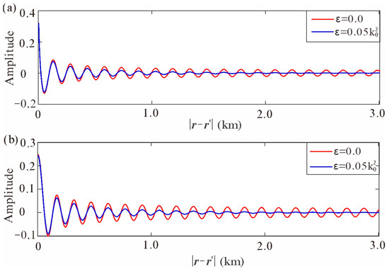
Figure 1. Amplitude decay curves of ${\widehat{G}}^{(0)}\left(\mathit{r},{\mathit{r}}^{\mathbf{\prime }}\right)$ for $\epsilon =0.0$ and $\epsilon =0.05k_0^2$ in a homogeneous medium. (a) Real part of ${\widehat{G}}^{(0)}\left(\mathit{r},{\mathit{r}}^{\mathbf{\prime }}\right)$; and (b) Imaginary part of ${\widehat{G}}^{(0)}\left(\mathit{r},{\mathit{r}}^{\mathbf{\prime }}\right)$.

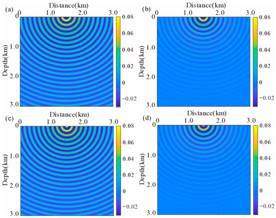
Figure 2. In 2-D Homogeneous Medium. (a) Real part of ${\widehat{G}}^{(0)}\left(\mathit{r},{\mathit{r}}^{\mathbf{\prime }}\right)$ for $\epsilon =0.0$; (b) Real part of ${\widehat{G}}^{(0)}\left(\mathit{r},{\mathit{r}}^{\mathbf{\prime }}\right)$ for $\epsilon =0.05k_0^2$; (c) Imaginary part of ${\widehat{G}}^{(0)}\left(\mathit{r},{\mathit{r}}^{\mathbf{\prime }}\right)$ for $\epsilon =0.0$; and (d) Imaginary part of ${\widehat{G}}^{(0)}\left(\mathit{r},{\mathit{r}}^{\mathbf{\prime }}\right)$ for $\epsilon =0.05k_0^2$.

Here, we analyze the selection principle of the damping factor $\epsilon$ given by Osnabrugge [25]:

$$\epsilon \ge {\max }_{\mathit{r}}\left|k^2(\mathit{r})-k_0^2\right|={\max }_{\mathit{r}}{k}_0^2\left|O(\mathit{r})\right|=k_0^2{\left|O\right|}_{\max }$$

(18)

where ${\left|O\right|}_{\max }$ is the maximum of the absolute value of $O\left(\mathit{r}\right)$. To design a strongly scattering medium with a model size of $3.0\mathrm{k}\mathrm{m}\times 3.0\mathrm{k}\mathrm{m}$, we consider a homogeneous medium with velocity $v_0=1500\mathrm{m}/\mathrm{s}$, within which is embedded a regular scatterer with velocity $v=4482\mathrm{m}/\mathrm{s}$ (Figure 3). We employ a single source located at ${\mathit{r}}^{\mathbf{\prime }}=(1500\mathrm{m},0\mathrm{m})$. Figure 4 and Figure 5 show the complex wavenumber background Green’s function ${\widehat{G}}^{(0)}\left(\mathit{r},{\mathit{r}}^{\mathbf{\prime }}\right)$ for a frequency of 20 Hz with $\epsilon =0.05k_0^2{\left|O\right|}_{\max }$ and $\epsilon =k_0^2{\left|O\right|}_{\max }$. It is evident from Figure 4 and Figure 5 that when $\epsilon =k_0^2{\left|O\right|}_{\max }$, the energy of the background Green’s function ${\widehat{G}}^{(0)}\left(\mathit{r},{\mathit{r}}^{\mathbf{\prime }}\right)$ rapidly decays near the source. The reason is that the wave speed of the optical medium differs from the seismic wave speed by several orders of magnitude. Furthermore, scattering contrast in the optical medium is relatively small. In the case of strong seismic scattering, it is clear that the damping factor $\epsilon$ calculated based on the selection principle proposed by Osnabrugge et al. [25] is not suitable. Therefore, it is necessary to reselect the damping factor $\epsilon$ to adapt to the seismic scattering problem.

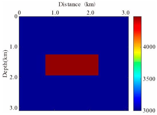
Figure 3. Regular single scattering model.

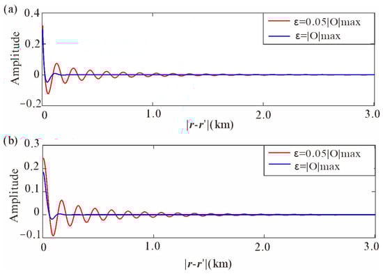
Figure 4. Amplitude decay curves of ${\widehat{G}}^{(0)}\left(\mathit{r},{\mathit{r}}^{\mathbf{\prime }}\right)$ for $\epsilon =0.05k_0^2{\left|O\right|}_{\max }$ and $\epsilon =k_0^2{\left|O\right|}_{\max }$ in a strongly scattering medium. (a) Real part of ${\widehat{G}}^{(0)}\left(\mathit{r},{\mathit{r}}^{\mathbf{\prime }}\right)$; and (b) Imaginary part of ${\widehat{G}}^{(0)}\left(\mathit{r},{\mathit{r}}^{\mathbf{\prime }}\right)$.

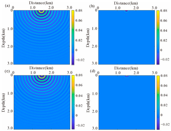
Figure 5. In a 2-D strongly scattering medium. (a) Real part of ${\widehat{G}}^{(0)}\left(\mathit{r},{\mathit{r}}^{\mathbf{\prime }}\right)$ for $\epsilon =0.05k_0^2{\left|O\right|}_{\max }$; (b) Real part of ${\widehat{G}}^{(0)}\left(\mathit{r},{\mathit{r}}^{\mathbf{\prime }}\right)$ for $\epsilon =k_0^2{\left|O\right|}_{\max }$; (c) Imaginary part of ${\widehat{G}}^{(0)}\left(\mathit{r},{\mathit{r}}^{\mathbf{\prime }}\right)$ for $\epsilon =0.05k_0^2{\left|O\right|}_{\max }$; and (d) Imaginary part of ${\widehat{G}}^{(0)}\left(\mathit{r},{\mathit{r}}^{\mathbf{\prime }}\right)$ for $\epsilon =k_0^2{\left|O\right|}_{\max }$.

The following is an analysis of the influence of selecting different damping factor $\epsilon$ values on iterative convergence and numerical solution of Green’s function. Considering the regular single scattering model in Figure 3, we compute the high-frequency source Green’s function $G\left(\mathit{r},{\mathit{r}}_s\right)$ at a frequency 50 Hz with ${\mathit{r}}_s=(1500\mathrm{m},0\mathrm{m})$. The iterative convergence relationship is shown in Figure 6 for the precondition $\gamma ={\gamma }_O$ and different damping factors $\epsilon$. It can be seen that with the increase of the value of $\epsilon$, the convergence speed is accelerated. The source Green’s function obtained by selecting different damping factors is shown in Figure 7a–c. When $\epsilon =1.0k_0^2|O{|}_{\max }$ and $\epsilon =0.5k_0^2|O{|}_{\max }$, the source Green’s function shows different degrees of energy attenuation, whereas, at $\epsilon =0.3k_0^2|O{|}_{\max }$, the numerical result better matches that obtained using the frequency domain finite difference (FDFD) method (Figure 7d).

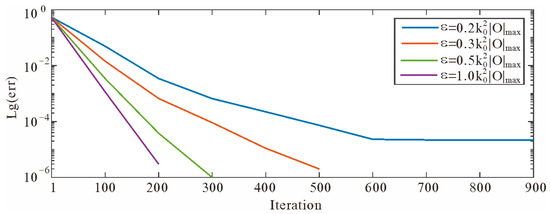
Figure 6. Analysis of the influence of different damping factor $\epsilon$ on iterative convergence.

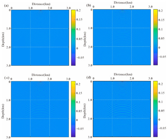
Figure 7. Analysis of the influence of different damping factors $\epsilon$ on the numerical solution of source Green’s function. (a) $\epsilon =1.0k_0^2|O{|}_{\max }$; (b) $\epsilon =0.5k_0^2|O{|}_{\max }$; (c) $\epsilon =0.3k_0^2|O{|}_{\max }$; (d) FDFD.

Building on the research conducted by Osnabrugge et al. [25], in this paper, the relationship between $\epsilon$ and the wave velocity perturbation $O\left(\mathit{r}\right)$ is preserved and the constant $a$ is introduced to establish a selection principle for the damping factor $\epsilon$ at the seismic exploration scale. The resulting equation is

$$\epsilon =a{k}_0^2{\left|O\right|}_{\max }(0\le a<1.0)$$

(19)

In numerical calculations, the damping factor $\epsilon$ may be adjusted by modifying the value of the constant $a$. For different models, it is necessary to test the influence of various $a$ values on the convergence of the iterative series and the numerical solution of Green’s function. This will enable us to choose an appropriate value of $a$ that yields optimal results.

3.2. Influence of $\gamma$ and Its Optimal Choice

When solving the Lippmann–Schwinger equation using the iterative method for a strongly scattering medium, the convergence rate is often quite slow or even diverges with increasing frequency. Although the GSOR iterative method can ensure convergence of the iterative series, it remains challenging to obtain a solution that satisfies the convergence error within a limited number of iterations when numerically solving for the high-frequency Green’s function. Hence, it is crucial to enhance the convergence of the iterative method. One way to achieve this is by identifying an appropriate preconditioning operator that can improve the frequency spectrum (eigenvalue) of the matrix operator $\widehat{L}$.

In the following analysis of the effect of Osnabrugge’s preconditioning operator ${\gamma }_O=\mathrm{i}\widehat{O}/\epsilon$ on the operator $\widehat{L}$, a selection principle is proposed for choosing a preconditioning operator that is suitable for a strongly scattering medium at the seismic exploration scale. We rewrite the operator from Equation (8) of the complex wavenumber L–S equation as

$$\widehat{L}G={\widehat{G}}_s^{(0)}$$

(20)

Using the left preconditioning operator for the above formula, the equivalent system of equations is expressed as

$$C^{-1}\widehat{L}G=C^{-1}(I-{\widehat{G}}^{(0)}\widehat{O})=C^{-1}{\widehat{G}}_s^{(0)}$$

(21)

We simplify Osnabrugge’s preconditioning operator as follows [25]:

$$C^{-1}={\gamma }_O=\frac{\mathrm{i}}{\epsilon }\widehat{O}=\frac{\mathrm{i}}{\epsilon }\left[k_0^{2}O(\mathit{r})-\mathrm{i}\epsilon \right]=1+\mathrm{i}\frac{k_0^{2}O(\mathit{r})}{\epsilon }$$

(22)

If $\epsilon =k_0^2{\left|O\right|}_{\max }$, the preconditioning operator is

$${\gamma }_O=1+\mathrm{i}\left[O(\mathit{r})/{\left|O\right|}_{\max }\right]$$

(23)

It can be seen from Equation (21) that in the matrix operator $\widehat{L}$, the background Green’s function discrete matrix operator ${\widehat{G}}^{(0)}$ is right-multiplied by the diagonal operator $\widehat{O}$, which is equivalent to scaling the matrix elements of ${\widehat{G}}^{(0)}$ by the columns. The preconditioning operator ${\gamma }_O$ is also a diagonal matrix operator. The left preconditioning operator ${\gamma }_O$ is applied to $\widehat{L}$, and its function is used to scale the matrix $\widehat{L}$ by the rows. This simple row weighting technique can balance the matrix elements, resulting in the new matrix having approximately the same $\infty$-norm. In practical applications, it is necessary to conduct specific analyses for different problems to select an appropriate weighting operator (diagonal preconditioner) [31].

Based on Osnabrugge’s preconditioning operator, we introduce a constant $b$, so that we can adjust the parameter $b$ to balance the elements of the matrix $\widehat{L}$. The following formula is used to calculate the preconditioning operator for the seismic exploration scale:

$$C^{-1}=\gamma =1+i\left[O(\mathit{r})/b{\left|O\right|}_{\max }\right],(b\ge 1.0)$$

(24)

For the regular single scattering model shown in Figure 3, with a given computation frequency of 50 Hz and $\epsilon =0.3k_0^2|O{|}_{\max }$, different constants $b$ were selected. The corresponding iterative convergence relationships under different diagonal preconditioners are shown in Figure 8. It can be observed that, compared to no preconditioning and preconditioners generated from the main diagonal elements of the matrix $\widehat{L}$, using the diagonal preconditioning selection principle of Equation (24) significantly improves the convergence of the iterative method after preconditioning. Moreover, the choice of different parameters $b$ affects the convergence speed of the iterative method, with $b=1.0$ yielding the best convergence rate in this example. Therefore, for different models, testing the impact of various parameters $b$ on the convergence of the iterative series allows for the selection of suitable parameters to generate preconditioners that accelerate the convergence rate of the numerical iterative method.

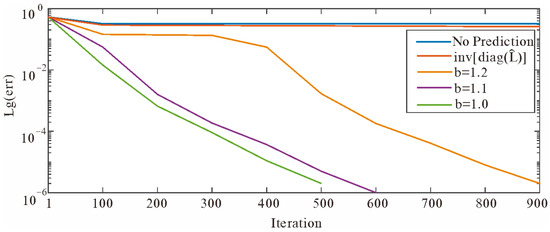
Figure 8. Convergence analysis of numerical iterative methods for source Green’s functions under different diagonal preconditioners.

4. Numerical Test

In this study, the effectiveness of the pre-GSOR iterative method for solving the complex wavenumber L–S equation was tested through numerical examples, and the convergence characteristics and computational efficiency were analyzed. Specifically, we used this method to compute the numerical Green’s function in a medium with strong velocity perturbations. The L–S equation was numerically discretized using the Nyström method with a weak singular kernel. To speed up the spatial convolution calculation during the iterative process, we employed a two-dimensional FFT [28]. In order to compare the numerical results of the pre-GSOR iterative method of the complex wavenumber L–S equation and frequency domain finite difference (FDFD) of the Helmholtz equation [32], we developed a single salt model with strong velocity perturbations and a resampled Society of Exploration Geophysics/European Association of Geoscientists and Engineers (SEG/EAGE) salt model with a smaller model scale. The numerical experimental environment consisted of a Linux operating system, four physical computational processing units (CPUs) with 16 cores each, and the CPU model utilized was the Intel(R) Xeon(R) Gold 6130 CPU @ 2.10 GHz.

4.1. Single Salt Model

First, we considered a simple model of a single salt combined with a homogeneous reference model (Figure 9). The model measured $3465\mathrm{m}\times 1050\mathrm{m}$ in width and depth, respectively, with grid intervals of $10\mathrm{m}\times 10\mathrm{m}$. The background wave speed v₀ was 2000 m/s. We employed a single source located at (1735 m, 0 m).

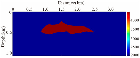
Figure 9. Single salt model.

The linear equation system $\widehat{L}G={\widehat{G}}^{(0)}$ stemming from the complex wavenumber L–S equation was solved using the pre-GSOR method. Table 1 presents the number of iterations required to meet the criterion of a normalized residual $err<{10}^{-6}$ for various values of a and b ($err=‖{\widehat{G}}^{(0)}-\widehat{L}{G}_n‖/‖{\widehat{G}}^{(0)}‖$). The maximum number of iterations was 1000. In the Pre-GSOR iterative method, we selected a = 0.5 and b = 1.0. At this point, the damping factor was $\epsilon =0.5k_0^2{\left|O\right|}_{\max }$ and the precondition operator was $\gamma (\mathit{r})=1.0+\mathrm{i}\left[O(\mathit{r})/1.0{\left|O\right|}_{\max }\right]$. Figure 10 shows the relationship between the normalized residual and the number of iterations obtained using the pre-GSOR iterative method of the complex wavenumber L–S equation and the GSOR iterative method of the real wavenumber L–S equation at frequencies of 30 Hz and 60 Hz. It is evident that the initial iteration error of the pre-GSOR iterative method is smaller, and it exhibits better convergence, even at high frequency.

Table 1. Number of iterations for various a and b values for the single salt model.

a	b	Frequency (f/Hz)
		10	20	30	40	50	60
0.4	1.0	190	314	>1000	>1000	>1000	>1000
	1.1	110	320	>1000	>1000	>1000	>1000
	1.2	105	360	>1000	>1000	>1000	>1000
0.5	1.0	142	300	672	>1000	>1000	>1000
	1.1	129	306	>1000	>1000	>1000	>1000
	1.2	121	323	>1000	>1000	>1000	>1000
0.6	1.0	183	303	459	585	713	733
	1.1	150	303	>1000	>1000	799	785
	1.2	141	309	>1000	>1000	>1000	>1000

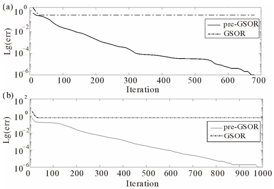
Figure 10. Curve of the normalized residual error versus the number of iterations (a = 0.5, b = 1.0). (a) 30 Hz Iteration-Lg(err) curve; and (b) 50 Hz Iteration-Lg(err) curve.

By comparing the numerical simulation results obtained using our algorithm with those obtained using the FDFD method, we obtained numerical solutions of Green’s function for frequencies of 30 Hz and 60 Hz (Figure 11 and Figure 12). It can be seen from Figure 11 that when the frequency is 30 Hz, the numerical results obtained using the two methods are basically the same and the error is small. When the frequency is 60 Hz (Figure 12), the numerical solution obtained using the pre-GSOR iterative method of the complex wavenumber L–S equation has a slight energy decay. A smaller constant a and more iterations may be required to completely match the FDFD numerical solution. However, for a strongly scattering medium, the complex wavenumber L–S equation pre-GSOR method still has good stability, and after a limited number of iterations, it has a high degree of agreement with the FDFD numerical solution.

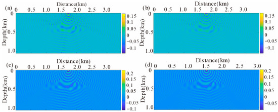
Figure 11. Numerical solution of Green’s function with a frequency of 30 Hz for a single salt model. (a) Real part of G (pre-GSOR); (b) Real part of G (FDFD); (c) Imaginary part of G (pre-GSOR); and (d) Imaginary part of G (FDFD).

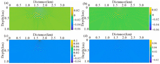
Figure 12. Numerical solution of Green’s function with a frequency of 50 Hz for a single salt model. (a) Real part of G (pre-GSOR); (b) Real part of G (FDFD); (c) Imaginary part of G (pre-GSOR); and (d) Imaginary part of G (FDFD).

4.2. SEG/EAGE Salt Model

Then, we considered the more complex SEG/EAGE salt model (Figure 13). The model was $6930\mathrm{m}\times 2100\mathrm{m}$ in width and depth directions, and the grid spacing was $10\mathrm{m}\times 10\mathrm{m}$. The background wave speed v₀ was 1500 m/s. We assumed that a single source was at the center of a single line at the top of the model.

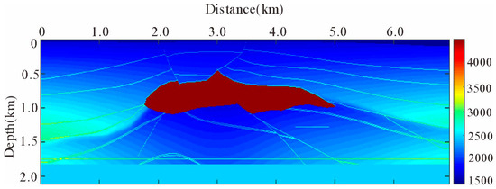
Figure 13. SEG/EAGE salt model.

Table 2 shows the number of iterations required for the normalized residual to satisfy $err<{10}^{-6}$ when different a and b values are chosen (the maximum number of iterations was set to 1000). To obtain an effective numerical solution, we chose $\epsilon =0.6k_0^2{\left|O\right|}_{\max }$ and $\gamma (\mathit{r})=1+i\left\{O(\mathit{r})/\left[2.0\ast {\left|O\right|}_{\max }\right]\right\}$. At this point, the energy of the Green’s function numerical solution obtained using the pre-GSOR iterative method of the complex wavenumber L–S equation did not decay too quickly.

Table 2. Number of iterations for various a and b values for the SEG/EAGE salt model.

a	b	Frequency (f/Hz)
		10	20	30	40	50
0.6	1.0	966	>1000	>1000	>1000	>1000
	2.0	768	>1000	>1000	503	211
	3.0	755	>1000	>1000	931	225
0.7	1.0	919	>1000	>1000	>1000	>1000
	2.0	758	976	864	412	163
	3.0	757	>1000	>1000	605	172
0.8	1.0	959	>1000	>1000	>1000	>1000
	2.0	763	896	711	353	133
	3.0	760	>1000	>1000	439	135

We selected certain frequencies during the frequency domain calculations and plotted the normalized residuals versus the number of iterations for the numerical solution of Green’s function. Figure 14 shows the relationship between the normalized residual and the number of iterations obtained using the pre-GSOR iterative method of the complex wavenumber L–S equation and the GSOR iterative method of the real wavenumber L–S equation when the frequency was 10 Hz and 30 Hz. It was found that when the model was more complex, the pre-GSOR iterative method of the complex wavenumber L–S equation requires more iterations to ensure convergence. However, our method still has a faster convergence speed than the GSOR iterative method of the real wavenumber L–S equation.

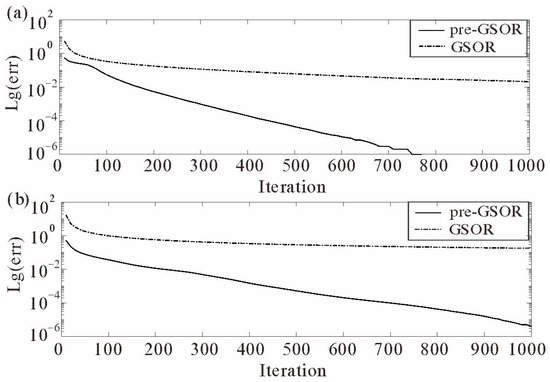
Figure 14. Curve of the normalized residual error versus the number of iterations (a = 0.6, b = 2.0). (a) 10 Hz Iteration-Lg(err) curve; and (b) 30 Hz Iteration-Lg(err) curve.

The real and imaginary parts of the numerical Green’s function solution were calculated using the pre-GSOR iterative method and the FDFD method at frequencies of 10 Hz and 30 Hz (Figure 15 and Figure 16, respectively). For strong scattering models with large model scales, the two methods could obtain consistent numerical results at low frequencies (Figure 15). At higher frequencies, our method had weak energy attenuation in the far field, but a satisfactory Green’s function numerical solution could still be obtained (Figure 16). It can be observed that for a strongly scattering medium, the pre-GSOR method not only has better stability but also has a high degree of matching with the FDTD numerical solution.

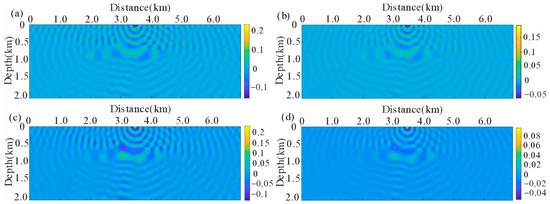
Figure 15. Numerical solution of Green’s function with a frequency of 10 Hz for the EAGE/SEG salt model. (a) Real part of G (pre-GSOR); (b) Real part of G (FDFD); (c) Imaginary part of G (pre-GSOR); and (d) Imaginary part of G (FDFD).

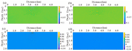
Figure 16. Numerical solution of Green’s function with a frequency of 30 Hz for the EAGE/SEG salt model. (a) Real part of G (pre-GSOR); (b) Real part of G (FDFD); (c) Imaginary part of G (pre-GSOR); and (d) Imaginary part of G (FDFD).

5. Analysis of Computation Efficiency and Memory Remand

The computational efficiency and memory usage of the proposed algorithm were evaluated. The matrix ${\widehat{G}}^{(0)}$ is an $N$-order ($N=N_x{N}_z$) square matrix. Obtaining sufficient memory to store the coefficient matrix on a microcomputer can be challenging, and the computational efficiency may not meet practical requirements. By analyzing the block Toeplitz properties of ${\widehat{G}}^{(0)}$, it is possible to reduce the storage of the matrix from $O(N^2)$ to $O(N)$. In addition, by utilizing the relationship between the block Toeplitz matrix and the block circulant matrix, the two-dimensional FFT can be employed to accelerate the matrix–vector product operation in the iterative process [28]. This approach can reduce the computational complexity of the matrix–vector product from $O(N^2)$ to $O(N\log N)$. Table 3 lists the CPU time required for solving the discrete equation and the memory storage size of the coefficient matrix during the numerical computation of the 2D single-frequency (30 Hz) source Green’s function using the Pre-GSOR method and the FDFD method. The results demonstrate that the fast numerical Green’s function calculation algorithm proposed in this paper requires minimal memory during the calculation process and achieves high computational efficiency. This provides an effective method for applying Green’s function in seismic inversion and migration imaging.

Table 3. CPU time and memory consumption for single Green’s function.

Model	Pre-GSOR		FDFD
	CPU Time (s)	Memory (M)	CPU Time (s)	Memory (M)
Single Salt	1.43	1.55	48.98	19.2
SEG/EAGE Salt	3.1	3.1	38.4	49.92

6. Conclusions

This paper presented a method for computing Green’s function in a strongly heterogeneous medium, called the generalized over-relaxation plus preconditioning method. The key point of the method is the combination of generalized over-relaxation and preconditioning to construct a successive approximation (scattering series) to the L–S equation in a slightly attenuated medium. First, we followed the idea of Osnabrugge et al. [25], introduced an imaginary component (damping factor) into the background wavenumber, and transformed the medium model from a non-attenuated one to a model with slight attenuation, obtaining an L–S equation with a complex wavenumber. Then, we modified the Born scattering series by combining the generalized over-relaxation presented in [27,29] and the preconditioning described in [25], obtaining an improved scattering series that is convergent for scattering in strongly inhomogeneous media. Next, we presented a detailed analysis of the influence of the damping factor and preconditioning operator on the numerical solution of Green’s function and provided a qualitative selection rule for these parameters in seismic applications. Numerical experiments showed that for a seismic strongly scattering medium, selecting an appropriate damping factor and preconditioning operator using the pre-GSOR iterative of the complex wavenumber L–S equation can not only obtain effective numerical solutions of Green’s function, but achieve better convergence of the iterative series. By utilizing the block Toeplitz property of the background Green’s operator, the memory requirements can be reduced. The matrix–vector product in the iterative process can be calculated using a two-dimensional FFT, which results in a high computational efficiency. Therefore, our pre-GSOR iterative method for computing Green’s function has potential applications in 3-D seismic forward modeling and inversion imaging.

References

- Sun, J. High-frequency asymptotic scattering theories and their applications in numerical modeling and imaging of geophysical fields: An overview of the research history and the state-of-the-art, and some new developments. J. Jilin Univ. (Earth Sci. Ed.) 2016, 46, 1231–1259. [Google Scholar]
- Cerveny, V. Seismic Ray Theory; Cambridge University Press: Cambridge, UK, 2001. [Google Scholar]
- Bleistein, N. Mathematical Methods for Wave Phenomena; USA Academic Press: Salt Lake City, UT, USA, 2012. [Google Scholar]
- Popov, M.M.; Semtchenok, N.M.; Popov, P.M.; Verdel, A.R. Depth migration by the Gaussian beam summation method. Geophysics 2010, 75, S81–S93. [Google Scholar] [CrossRef]
- Shi, X.; Sun, J.; Sun, H.; Liu, M.; Liu, Z. The time-domain depth migration by the summation of delta packets. Chin. J. Geophys. 2016, 59, 2641–2649. [Google Scholar]
- Sun, J. The history, the state of the art and the future trend of the research of Kirchhoff-type migration theory: A comparison with optical diffraction theory, some new result and new understanding, and some problems to be solved. J. Jilin Univ. (Earth Sci. Ed.) 2012, 42, 1521–1552. [Google Scholar]
- Huang, X.; Sun, H.; Sun, J. Born modeling for heterogeneous media using the Gaussian beam summation based Green’s function. J. Appl. Geophys. 2016, 131, 191–201. [Google Scholar] [CrossRef]
- Huang, X.; Sun, J.; Sun, Z. Local algorithm for computing complex travel time based on the complex eikonal equation. Phys. Rev. E 2016, 93, 043307. [Google Scholar] [CrossRef] [PubMed]
- Huang, X. Integral equation methods with multiple scattering and Gaussian beams in inhomogeneous background media for solving nonlinear inverse scattering problems. IEEE Trans. Geosci. Remote Sens. 2020, 59, 5345–5351. [Google Scholar] [CrossRef]
- Schuster, G.T. Reverse-time migration = generalized diffraction stack migration. In Proceedings of the SEG International Exposition and Annual Meeting, Salt Lake City, UT, USA, 6 October 2002. [Google Scholar]
- Schuster, G.T. Seismic Inversion; Society of Exploration Geophysicists: Yulsa, OK, USA, 2017. [Google Scholar]
- Zhang, G. Generalized Diffraction-Stack Migration. Ph.D. Thesis, The University of Utah, Salt Lake City, UT, USA, 2012. [Google Scholar]
- Zhang, G.; Dai, W.; Zhou, M.; Luo, Y.; Schuster, G.T. Generalized diffraction-stack migration and filtering of coherent noise. Geophys. Prospect. 2014, 62, 427–442. [Google Scholar] [CrossRef]
- Wu, R.S. Wave propagation, scattering and imaging using dual-domain one-way and one-return propagators. Pure Appl. Geophys. 2003, 160, 509–539. [Google Scholar] [CrossRef]
- Wu, R.; Xie, X.; Wu, X. One-way and one-return approximations (De Wolf approximation) for fast elastic wave modeling in complex media. Adv. Geophys. 2007, 48, 265–322. [Google Scholar]
- Innanen, K.A. Born series forward modelling of seismic primary and multiple reflections: An inverse scattering shortcut. Geophys. J. Int. 2009, 177, 1197–1204. [Google Scholar] [CrossRef]
- Jakobsen, M.; Wu, R. Renormalized scattering series for frequency-domain waveform modelling of strong velocity contrasts. Geophys. J. Int. 2016, 206, 880–899. [Google Scholar] [CrossRef]
- Huang, L.; Fehler, M.; Zheng, Y.; Xie, X.B. Seismic-Wave Scattering, Imaging, and Inversion. Commun. Comput. Phys. 2020, 28, 1–40. [Google Scholar]
- Jakobsen, M. T-matrix approach to seismic forward modelling in the acoustic approximation. Stud. Geophys. Geod. 2012, 56, 1–20. [Google Scholar] [CrossRef]
- Eftekhar, R.; Hu, H.; Zheng, Y. Convergence acceleration in scattering series and seismic waveform inversion using non-linear Shanks transformation. Geophys. J. Int. 2018, 214, 1732–1743. [Google Scholar] [CrossRef]
- Huang, K. A critical history of renormalization. Int. J. Mod. Phys. A 2013, 28, 1330050. [Google Scholar] [CrossRef]
- Jakobsen, M.; Wu, R. Accelerating the T-matrix approach to seismic full-waveform inversion by domain decomposition. Geophys. Prospect. 2018, 66, 1039–1059. [Google Scholar] [CrossRef]
- Jakobsen, M.; Wu, R.S.; Huang, X.G. Seismic waveform modeling in strongly scattering media using renormalization group theory. In Proceedings of the SEG International Exposition and Annual Meeting, Anaheim, CA, USA, 14 October 2018. [Google Scholar]
- Jakobsen, M.; Wu, R.; Huang, X. Convergent scattering series solution of the inhomogeneous Helmholtz equation via renormalization group and homotopy continuation approaches. J. Comput. Phys. 2020, 409, 109343. [Google Scholar] [CrossRef]
- Osnabrugge, G.; Leedumrongwatthanakun, S.; Vellekoop, I.M. A convergent Born series for solving the inhomogeneous Helmholtz equation in arbitrarily large media. J. Comput. Phys. 2016, 322, 113–124. [Google Scholar] [CrossRef]
- Huang, X.; Jakobsen, M.; Wu, R. On the applicability of a renormalized Born series for seismic wavefield modelling in strongly scattering media. J. Geophys. Eng. 2020, 17, 277–299. [Google Scholar] [CrossRef]
- Xu, Y.; Sun, J.; Shang, Y.; Meng, X.; Wei, P. The generalized over-relaxation iterative method for Lippmann-Schwinger equation and its convergence. Chin. J. Geophys. 2021, 64, 249–262. [Google Scholar]
- Xu, Y.; Sun, J.; Shang, Y. A parallel computation method for scattered seismic waves using Nyström discretization and FFT fast convolution. Chin. J. Geophys. 2021, 64, 2877–2887. [Google Scholar]
- Petryshyn, W.V. On a general iterative method for the approximate solution of linear operator equations. Math. Comput. 1963, 17, 1–10. [Google Scholar] [CrossRef]
- Kleinman, R.E.; Van den Berg, P.M. Iterative methods for solving integral equations. Radio Sci. 1991, 26, 175–181. [Google Scholar] [CrossRef]
- Golub, G.H.; Van Loan, C.F. Matrix Computations, 4th ed.; Johns Hopkins University Press: Baltimore, MD, USA, 2013. [Google Scholar]
- Hondori, E.J.; Mikada, H.; Goto, T.N.; Takekawa, J. A MATLAB Package for Frequency Domain Modeling of Elastic Waves. In Proceedings of the 75th EAGE Conference & Exhibition Incorporating SPE EUROPEC, London, UK, 10–13 June 2013. [Google Scholar]
Disclaimer/Publisher’s Note: The statements, opinions and data contained in all publications are solely those of the individual author(s) and contributor(s) and not of MDPI and/or the editor(s). MDPI and/or the editor(s) disclaim responsibility for any injury to people or property resulting from any ideas, methods, instructions or products referred to in the content. |
© 2024 by the authors. Licensee MDPI, Basel, Switzerland. This article is an open access article distributed under the terms and conditions of the Creative Commons Attribution (CC BY) license (https://creativecommons.org/licenses/by/4.0/).