Bifurcation Analysis of a Class of Two-Delay Lotka–Volterra Predation Models with Coefficient-Dependent Delay

Abstract

In this paper, a class of two-delay differential equations with coefficient-dependent delay is studied. The distribution of the roots of the eigenequation is discussed, and conditions for the stability of the internal equilibrium and the existence of Hopf bifurcation are obtained. Additionally, using the normal form method and the central manifold theory, the bifurcation direction and the stability for the periodic solution of Hopf bifurcation are calculated. Finally, the correctness of the theory is verified by numerical simulation.

1. Introduction

The interaction between species in ecosystems is one of the core contents of ecological research. In population ecology, species relationships include parasitic, reciprocal, competitive, and predator–prey interactions. Notably, the interaction between predators and prey plays a significant role in maintaining ecosystem stability and diversity. The Lotka–Volterra model

$$\left\{\begin{array}{l}\dot{x}\left(t\right)=x\left(t\right)\left(r-by\left(t\right)\right),\\ \dot{y}\left(t\right)=\alpha x\left(t\right)y\left(t\right)-vy\left(t\right)\end{array}\right.$$

(1)

is a classic predator–prey model widely used to describe the interactions between predators and prey. In this model, $x\left(t\right)$ and $y\left(t\right)$ represent the population density of prey and predators, respectively. The parameter $r$ indicates the birth rate of the prey population, $b$ indicates the success rate of predators’ predation of prey, $\alpha$ represents the nutritional conversion coefficient of the predators, and $v$ represents the mortality rate of predators. In the original Lotka–Volterra predator–prey model (1), it is assumed that the growth of prey populations is affected by the intrinsic growth rate and predation pressure from predators and that the growth of predator populations is affected by their feeding rates and their natural mortality rates. In order to describe the interaction between populations more realistically, the following model is proposed considering the density constraint effect within populations:

$$\left\{\begin{array}{l}\dot{x}\left(t\right)=x\left(t\right)\left(r-ax\left(t\right)-by\left(t\right)\right),\\ \dot{y}\left(t\right)=\alpha x\left(t\right)y\left(t\right)-vy\left(t\right)-\beta y^2\left(t\right),\end{array}\right.$$

(2)

where $a$ indicates the constraint coefficient of the prey population density, $\beta$ represents the constraint coefficient of the predators’ population density, and $r,b,\alpha ,v$ have the same biological significance as model (1).

In model (2), it is usually assumed that all individuals have the same degree of survival and predation ability and that the interaction between organisms is instantaneous, so there was no time delay, which is often not true in actual ecosystems. Considering that biological individuals usually have a growth and development process, it becomes necessary to consider the time delay effect between predators and prey. Time delay effect refers to the delay caused by physiological processes such as the growth, reproduction, and migration of biological individuals. Therefore, studying Lotka–Volterra predator–prey models with time delays helps to better understand the interactions between predators and prey in actual ecosystems, providing a theoretical basis for ecological protection and management. In order to more accurately describe and predict the changing trends of species populations with obvious seasonal or life cycle characteristics, researchers have incorporated time delay effects into the Lotka–Volterra predation model [1,2,3,4]. Most scholars have considered the single time delay effect [5,6]; for instance, May proposes the following model [7]:

$$\left\{\begin{array}{l}\dot{x}\left(t\right)=x\left(t\right)\left(r-ax\left(t-\tau \right)-by\left(t\right)\right),\\ \dot{y}\left(t\right)=\alpha x\left(t\right)y\left(t\right)-vy\left(t\right)-\beta y^2\left(t\right),\end{array}\right.$$

(3)

where $\tau$ indicates the pregnancy time of the prey population.

Due to the different predatory abilities of predators at different stages, it takes time for juvenile predators to grow into adult predators. Therefore, incorporating these stage structures into predator models can provide a more accurate description of the relationship between predators and prey in ecosystems. Populations are typically divided into several stages according to certain physiological characteristics, such as juvenile, adult and old age. Corresponding stage-structured models are established for research purposes, which may result in new dynamic behaviors [8,9,10]. Assuming that the growth of the prey population follows Lotka–Volterra and that the young predators are unable to prey on the prey and are unable to reproduce, Xu proposes the following model [11]:

$$\left\{\begin{array}{l}\dot{x}\left(t\right)=x\left(t\right)\left(r-ax\left(t\right)-b{y}_2\left(t\right)\right),\\ {\dot{y}}_1\left(t\right)=\alpha x\left(t\right)y_2\left(t\right)-d{y}_1\left(t\right)-\alpha e^{-d\tau }x\left(t-\tau \right)y_2\left(t-\tau \right),\\ {\dot{y}}_2\left(t\right)=\alpha e^{-d\tau }x\left(t-\tau \right)y_2\left(t-\tau \right)-v{y}_1\left(t\right)-\beta y_2^2\left(t\right),\end{array}\right.$$

(4)

where $x\left(t\right)$ represents the population density of prey, $y_1\left(t\right)$ represents the population density of juvenile predators, $y_2\left(t\right)$ represents the population density of adult predators, $r,a,b,\alpha ,\beta$ have the same biological significance as model (2), $v$ represents the mortality rate of the adult predator population, $d$ indicates the mortality rate of juvenile predators, $\tau$ indicates the time when juvenile predators mature, and $\alpha e^{-d{\tau }_2}x\left(t-\tau \right)y\left(t-\tau \right)$ indicates at the moment of $t-\tau$, the population density of juvenile predators reproduced by adult predators that survive after the time of $\left[t-\tau ,t\right]$. Based on previous studies, this article considers the Lotka–Volterra predator–prey model with a stage structure including pregnancy delay, as follows:

$$\left\{\begin{array}{l}\dot{x}\left(t\right)=x\left(t\right)\left(r-ax\left(t-{\tau }_1\right)-b{y}_2\left(t\right)\right),\\ {\dot{y}}_1\left(t\right)=\alpha x\left(t-{\tau }_1\right)y_2\left(t\right)-d{y}_1\left(t\right)-\alpha e^{-d{\tau }_2}x\left(t-{\tau }_2\right)y\left(t-{\tau }_2\right),\\ {\dot{y}}_2\left(t\right)=\alpha e^{-d{\tau }_2}x\left(t-{\tau }_2\right)y\left(t-{\tau }_2\right)-v{y}_1\left(t\right)-\beta y_2^2\left(t\right).\end{array}\right.$$

(5)

In model (5), the first and third equations do not contain variables $y_1$, meaning that they are not coupled with the second equation; therefore, we only need to consider the following models:

$$\left\{\begin{array}{l}\dot{x}\left(t\right)=x\left(t\right)\left(r-ax\left(t-{\tau }_1\right)-by\left(t\right)\right),\\ \dot{y}\left(t\right)=\alpha e^{-d{\tau }_2}x\left(t-{\tau }_2\right)y\left(t-{\tau }_2\right)-vy\left(t\right)-\beta y^2\left(t\right),\end{array}\right.$$

(6)

where $x\left(t\right)$ represents the population density of prey, $y\left(t\right)$ represents the population density of adult predators, $r,a,b,\alpha ,v,\beta ,d$ are all positive numbers with the same biological significance as model (4), ${\tau }_1$ indicates the pregnancy time of the prey population, ${\tau }_2$ indicates the time when juvenile predators mature, and $\alpha e^{-d{\tau }_2}x\left(t-{\tau }_2\right)y\left(t-{\tau }_2\right)$ indicates at the moment of $t-{\tau }_2$, the population density of juvenile predators reproduced by adult predators that survive after the time of $\left[t-{\tau }_2,t\right]$. First, this paper studied five different scenarios based on different values of two time delays and provided stability analysis for internal equilibrium and the existence of Hopf bifurcation in these scenarios. Second, using normal form method and central manifold theory, we determined the direction of branching for Hopf bifurcation and analyzed the stability of periodic solutions. Finally, numerical simulations were conducted using Matlab to verify the theoretical findings.

2. Hopf Bifurcation Analysis

By making the right-hand function of system (6) equal to 0, the internal equilibrium of system (6) can be obtained as $E^{\ast }\left(x^{\ast },y^{\ast }\right)$, where:

$$x^{\ast }=\frac{bv+\beta r}{\alpha e^{-d{\tau }_2}+a\beta },y^{\ast }=\frac{\alpha e^{-d{\tau }_2}-av}{\alpha e^{-d{\tau }_2}+a\beta }$$

When $\left(H_1\right)\alpha e^{-d{\tau }_2}-av>0$ is true, system (6) has a positive internal equilibrium.

The linearization of system (6) at $E^{\ast }\left(x^{\ast },y^{\ast }\right)$ is as follows:

$$\left\{\begin{array}{l}\dot{x}\left(t\right)=rx\left(t\right)-a{x}^{\ast }x\left(t-{\tau }_1\right)-a{x}^{\ast }x\left(t\right)-b{x}^{\ast }y\left(t\right)-b{y}^{\ast }x\left(t\right),\\ \dot{y}\left(t\right)=\alpha e^{-d{\tau }_2}{x}^{\ast }y\left(t-{\tau }_2\right)+\alpha e^{-d{\tau }_2}{y}^{\ast }x\left(t-{\tau }_2\right)-vy\left(t\right)-2\beta y^{\ast }y\left(t\right).\end{array}\right.$$

(7)

The characteristic equation associated with (7) is:

$$\left|\begin{array}{cc}\lambda -r+a{x}^{\ast }+\alpha x^{\ast }{e}^{-\lambda {\tau }_1}+b{y}^{\ast }& b{x}^{\ast }\\ -\alpha e^{-d{\tau }_2}{y}^{\ast }{e}^{-\lambda {\tau }_2}& \lambda -\alpha e^{-d{\tau }_2}{x}^{\ast }{e}^{-\lambda {\tau }_2}+v+2\beta y^{\ast }\end{array}\right|=0$$

i.e.,

$${\lambda }^2+p_1\lambda +e^{-\lambda {\tau }_1}\left(p_2\lambda +p_3\right)+e^{-\lambda {\tau }_2}\left(p_4\lambda +p_5\right)+p_6{e}^{-\lambda \left({\tau }_1+{\tau }_2\right)}=0,$$

(8)

where:

$$p_1=v+2\beta y^{\ast },p_2=a{x}^{\ast },p_3=a{x}^{\ast }\left(v+2\beta y^{\ast }\right),$$

$$p_4=-\alpha e^{-d{\tau }_2}{x}^{\ast },p_5=\alpha e^{-d{\tau }_2}{x}^{\ast }b{y}^{\ast },p_6=-a\alpha e^{-d{\tau }_2}{\left(x^{\ast }\right)}^2.$$

Below, five different scenarios were discussed on the stability of system (6) at $E^{\ast }\left(x^{\ast },y^{\ast }\right)$ and the existence of Hopf bifurcation.

Case 1. ${\tau }_1={\tau }_2=0$.

In this case, Equation (8) becomes:

$${\lambda }^2+\left(p_1+p_2+p_4\right)\lambda +p_3+p_5+p_6=0.$$

For convenience, provide the assumption $\left(H_2\right)p_1+p_2+p_4>0\wedge p_3+p_5+p_6>0$.

According to the Routh–Hurwitz criterion, the following theorem can be obtained.

Theorem 1.

If $\left(H_1\right)$ and $\left(H_2\right)$ are true, then the internal equilibrium $E^{\ast }\left(x^{\ast },y^{\ast }\right)$ of system (6) is asymptotically stable.

Case 2. ${\tau }_1=0,{\tau }_2>0.$

Equation (8) becomes:

$${\lambda }^2+\left(p_2+p_1\right)\lambda +p_3+e^{-\lambda {\tau }_2}\left(p_4\lambda +p_5+p_6\right)=0,$$

(9)

let

$$p_{11}=p_2+p_1,q_{11}=p_4,a\left({\tau }_2\right)=p_3,b\left({\tau }_2\right)=p_5+p_6,$$

$$P\left(\lambda ,{\tau }_2\right)={\lambda }^2+p_{11}\lambda +a\left({\tau }_2\right),Q\left(\lambda ,{\tau }_2\right)=q_{11}\lambda +b\left({\tau }_2\right).$$

Equation (9) becomes:

$$P\left(\lambda ,{\tau }_2\right)+e^{-\lambda {\tau }_2}Q\left(\lambda ,{\tau }_2\right)=0.$$

(10)

One can obtain ${\tau }_2<\frac{1}{d}ln\frac{\alpha r}{av}$ from $\left(H_1\right)$; denote ${\tau }_{max}=\frac{1}{d}ln\frac{\alpha r}{av}$.

According to the geometric criteria in [12], the following five conditions are verified for Equation (10):

(i)

$P\left(0,{\tau }_2\right)+Q\left(0,{\tau }_2\right)\ne 0,\forall {\tau }_2\in R_{+;}$

(ii)

$P\left(i\omega ,{\tau }_2\right)+Q\left(i\omega ,{\tau }_2\right)\ne 0,\forall \omega \in R,\forall {\tau }_2\in R_{+;}$

(iii)

$\underset{\left|\lambda \right|\to \mathrm{\infty }}{\mathit{lim}}\left\{\left|\frac{Q\left(\lambda ,{\tau }_2\right)}{P\left(\lambda ,{\tau }_2\right)}\right|:\mathfrak{R}\lambda \ge 0\right\}<1,\forall {\tau }_2\in R_{+;}$

(iv)

$\forall {\tau }_2,F\left(\omega ,{\tau }_2\right):={\left|P\left(i\omega ,{\tau }_2\right)\right|}^2-{\left|Q\left(i\omega ,{\tau }_2\right)\right|}^2$ has at most a finite number of real zeros;

(v)

Each positive root $\omega \left({\tau }_2\right)$ of $F\left(\omega ,{\tau }_2\right)=0$ is continuous and differentiable in ${\tau }_2$ whenever it exists.

Obviously, the condition (v) is valid. When $\lambda =0$, if $\left(H_2\right)$ is true, one can obtain $P\left(0,{\tau }_2\right)+Q\left(0,{\tau }_2\right)=a\left({\tau }_2\right)+b\left({\tau }_2\right)>0$, so the condition (i) is valid. When $\omega \ne 0$:

$$P\left(i\omega ,{\tau }_2\right)+Q\left(i\omega ,{\tau }_2\right)={-\omega }^2+i{p}_{11}\omega +a\left({\tau }_2\right)+i{q}_{11}\omega +b\left({\tau }_2\right).$$

If $\left(H_2\right)$ is true, $p_{11}+q_{11}=p_1+p_2+p_4>0$, so $P\left(i\omega ,{\tau }_2\right)+Q\left(i\omega ,{\tau }_2\right)\ne 0$. When $\omega =0$, condition (ii) is the same as condition (i), that is, condition (ii) is true. Because:

$$\underset{\left|\lambda \right|\to \infty }{\mathit{lim}}\left|\frac{Q\left(\lambda ,{\tau }_2\right)}{P\left(\lambda ,{\tau }_2\right)}\right|=\frac{q_{11}\lambda +b\left({\tau }_2\right)}{{\lambda }^2+p_{11}\lambda +a\left({\tau }_2\right)}=0<1,$$

the condition (iii) is true. From:

$${\left|P\left(i\omega ,{\tau }_2\right)\right|}^2={\left({\omega }^2-a\left({\tau }_2\right)\right)}^2+p_{11}^2{\omega }^2,$$

$${\left|Q\left(i\omega ,{\tau }_2\right)\right|}^2=b^2\left({\tau }_2\right)+q_{11}^2{\omega }^2,$$

one can obtain:

$$F\left(\omega ,{\tau }_2\right)={\omega }^4+\left(p_{11}^2-2a\left({\tau }_2\right)-q_{11}^2\right){\omega }^2+a^2\left({\tau }_2\right)-b^2\left({\tau }_2\right).$$

(11)

Therefore, $F\left(\omega ,{\tau }_2\right)$ has at most four roots, so condition (iv) is true.

To make $F\left(\omega ,{\tau }_2\right)$ have a positive root, define the set according to (11):

$$I_1=\left\{{\tau }_2\vee \left|a\left({\tau }_2\right)\right|<\left|b\left({\tau }_2\right)\right|,\forall {\tau }_2\in \left[0,{\tau }_{max}\right]\right\}.$$

When ${\tau }_2\in I_1,F\left(\omega ,{\tau }_2\right)$ has a positive real zero point ${\omega }_0\left({\tau }_2\right)$, where:

$${\omega }_0\left({\tau }_2\right)=\sqrt{\frac{-\left(p_{11}^2-2a\left({\tau }_2\right)-q_{11}^2\right)+\sqrt{{\left(p_{11}^2-2a\left({\tau }_2\right)-q_{11}^2\right)}^2-4\left(a^2\left({\tau }_2\right)-b^2\left({\tau }_2\right)\right)}}{2}}.$$

When ${\tau }_2>0$, assume $\pm i\omega$ is the pure imaginary root of Equation (9), substitute $\lambda =i\omega \left(\omega >0\right)$ into Equation (9) and separate the real and imaginary parts to obtain:

$$\left\{\begin{array}{l}-{\omega }^2+a\left({\tau }_2\right)+b\left({\tau }_2\right)cos\left(\omega {\tau }_2\right)+q_{11}\omega sin\left(\omega {\tau }_2\right)=0,\\ p_{11}\omega +q_{11}\omega cos\left(\omega {\tau }_2\right)-b\left({\tau }_2\right)sin\left(\omega {\tau }_2\right)=0.\end{array}\right.$$

(12)

So one can obtain:

$$sin\left(\omega {\tau }_2\right)=\frac{-\left(-{\omega }^2+a\left({\tau }_2\right)\right)q_{11}\omega +p_{11}\omega b\left({\tau }_2\right)}{b^2\left({\tau }_2\right)+q_{11}^2{\omega }^2},$$

$$cos\left(\omega {\tau }_2\right)=\frac{-\left(-{\omega }^2+a\left({\tau }_2\right)\right)b\left({\tau }_2\right)+p_{11}{q}_{11}{\omega }^2}{b^2\left({\tau }_2\right)+q_{11}^2{\omega }^2}.$$

The following can be concluded from (12):

$${\left(-{\omega }^2+a\left({\tau }_2\right)\right)}^2+{\left(p_{11}\omega \right)}^2={\left(b\left({\tau }_2\right)\right)}^2+{\left(q_{11}\omega \right)}^2.$$

This equation is the same as $F\left(\omega ,{\tau }_2\right)=0$, because $F\left(\omega ,{\tau }_2\right)$ has a positive root, Equation (9) has a pair of simple pure imaginary roots $\pm i\omega$. When ${\tau }_2\in I_1$, make $\omega \left({\tau }_2\right){\tau }_2=\theta \left({\tau }_2\right)+2n\pi$ and $S_n\left({\tau }_2\right)={\tau }_2-\frac{\theta \left({\tau }_2\right)+2n\pi }{\omega \left({\tau }_2\right)}$, so $\pm i\omega \left({\tau }_2\right)$ is the pure imaginary root of Equation (9); if and only if ${\tau }_2$ is the root of $S_n\left({\tau }_2\right)=0$, write ${\tau }_2^{\left(j\right)}$ as the root of $S_n\left({\tau }_2\right)=0$. The following theorem can be obtained from Theorem 2.2 in [12].

Theorem 2.

When ${\tau }_2\in I_1$ , if there is $S_n\left({\tau }_2^{\left(j\right)}\right)=0\left(n\in N\right)$ at ${\tau }_2={\tau }_2^{\left(j\right)}$ , when there is ${\tau }_2={\tau }_2^{\left(j\right)}$ Equation (9) has a pair of pure imaginary roots, that is $\pm i\omega \left({\tau }_2^{\left(j\right)}\right)$ , and if $\delta \left({\tau }_2^{\left(j\right)}\right)>0\left(<0\right)$ , so when ${\tau }_2$ increases and crosses ${\tau }_2^{\left(j\right)}$, the roots corresponding to this pair of pure imaginary roots will cross the imaginary axis from the left (right) half plane of the complex plane to the right (left) half plane, where:

$$\delta \left({\tau }_2^{\left(j\right)}\right)=sign\left\{{\left.\frac{d\mathfrak{R}\lambda \left({\tau }_2\right)}{d{\tau }_2}\right|}_{{\tau }_2={\tau }_2^{\left(j\right)}}\right\}=sign\left\{F_{\omega }^{\prime }\left(\omega \left({\tau }_2^{\left(j\right)}\right),{\tau }_2^{\left(j\right)}\right)\right\}sign\left\{{\left.\frac{d{S}_n\left({\tau }_2\right)}{d{\tau }_2}\right|}_{{\tau }_2={\tau }_2^{\left(j\right)}}\right\}.$$

(13)

Due to:

$$p_{11}^2-2a\left({\tau }_2\right)-q_{11}^2=\left(p_1+p_2+p_4\right)\left(p_1+p_2-p_4\right)-2p_3$$

$$=p_1^2+p_2^2+p_4^2-2p_1{p}_4-2p_2{p}_4>0,$$

therefore:

$$F_{\omega }^{\prime }\left(\omega \left({\tau }_2^{\left(j\right)}\right),{\tau }_2^{\left(j\right)}\right)=4{\omega }^3+2\left(p_{11}^2-2a\left({\tau }_2\right)-q_{11}^2\right)\omega >0.$$

Thus, (13) is equivalent to:

$$\delta \left({\tau }_2^{\left(j\right)}\right)=sign\left\{{\left.\frac{d\mathfrak{R}\lambda \left({\tau }_2\right)}{d{\tau }_2}\right|}_{{\tau }_2={\tau }_2^{\left(j\right)}}\right\}=sign\left\{{\left.\frac{d{S}_n\left({\tau }_2\right)}{d{\tau }_2}\right|}_{{\tau }_2={\tau }_2^{\left(j\right)}}\right\}.$$

(14)

It is easy to know when ${\tau }_2\in I_1,S_n\left({\tau }_2\right)$ is monotonically decreasing with respect to $n$, that is $S_n\left({\tau }_2\right)<S_{n+1}\left({\tau }_2\right);$ if $S_0\left({\tau }_2\right)$ has no zero point, $S_n\left({\tau }_2\right)\left(\forall n\in N\right)$ has no zero point, either. When ${\tau }_2=0$, obviously $S_0\left({\tau }_2\right)<0$. When ${\tau }_2\to {\tau }_{max},a\left({\tau }_2\right)+b\left({\tau }_2\right)\to 0$, so $\omega \left({\tau }_2\right)\to 0$. Additionally, according to $sin\left(\omega {\tau }_2\right)\to 0$, $cos\left(\omega {\tau }_2\right)\to 1$, one can know that $\theta \left({\tau }_2\right)\to 2\pi$, so $S_0\left({\tau }_2\right)\to -\infty$. Therefore, $S_n\left({\tau }_2\right)\left(\forall n\in N\right)$ intersects with the horizontal axis, and the number of intersections is even. Let the intersection be:

$${\tau }_2^{min}\triangleq {\tau }_2^{\left(1\right)}<{\tau }_2^{\left(2\right)}<{\tau }_2^{\left(3\right)}<\cdots <{\tau }_2^{\left(j\right)}\triangleq {\tau }_2^{max},$$

where j is an even number.

Theorem 3.

When ${\tau }_2\in I_1$ , if $\left(H_1\right),\left(H_2\right)$ is true, then:

(1) If $S_0\left({\tau }_2\right)$ has no zero point, then the internal equilibrium $E^{\ast }\left(x^{\ast },y^{\ast }\right)$ is asymptotically stable.

(2) If $S_0\left({\tau }_2\right)$ has at least one positive root, then there exists ${\tau }_2^{\left(1\right)}$ so that when ${\tau }_2\in [0, {\tau }_2^{\left(1\right)})$, the internal equilibrium $E^{\ast }\left(x^{\ast },y^{\ast }\right)$ of system (6) is asymptotically stable. When ${\tau }_2\in \left({\tau }_2^{\left(1\right)},{\tau }_2^{max}\right)$, the internal equilibrium $E^{\ast }\left(x^{\ast },y^{\ast }\right)$ of system (6) is not stable. When ${\tau }_2\in \left({\tau }_2^{max},{\tau }_{max}\right)$, the internal equilibrium $E^{\ast }\left(x^{\ast },y^{\ast }\right)$ of system (6) is asymptotically stable. When ${\tau }_2={\tau }_2^{\left(j\right)}\left(j=\mathrm{1,2},\cdots \right)$, system (6) has a Hopf bifurcation at $E^{\ast }\left(x^{\ast },y^{\ast }\right)$.

Case 3. ${\tau }_1>0,{\tau }_2\in \left(0,{\tau }_2^{\left(1\right)}\right),$ fix ${\tau }_2$ within a stable interval and discuss ${\tau }_1$ as a parameter.

Substitute $\lambda =i\omega \left(\omega >0\right)$ into Equation (8) and separate the real and imaginary parts to obtain:

$$\left\{\begin{array}{l}-{\omega }^2+p_{3}cos\left(\omega {\tau }_1\right)+p_2\omega sin\left(\omega {\tau }_1\right)+p_{5}cos\left(\omega {\tau }_2\right)+\wedge p_4\omega sin\left(\omega {\tau }_2\right)+p_{6}cos\left(\omega {\tau }_1\right)cos\left(\omega {\tau }_2\right)-p_{6}sin\left(\omega {\tau }_1\right)sin\left(\omega {\tau }_2\right)=0,\\ p_1\omega +p_2\omega cos\left(\omega {\tau }_1\right)-p_{3}sin\left(\omega {\tau }_1\right)+p_4\omega cos\left(\omega {\tau }_2\right)-\wedge p_{5}sin\left(\omega {\tau }_2\right)-p_{6}sin\left(\omega {\tau }_1\right)cos\left(\omega {\tau }_2\right)-p_{6}cos\left(\omega {\tau }_1\right)sin\left(\omega {\tau }_2\right)=0.\end{array}\right.$$

(15)

From (15), we can obtain the following equation about $\omega$:

$${\omega }^4+{M_1\omega }^3+{M_2\omega }^2+M_3\omega +M_4=0,$$

(16)

where:

$$M_1=-2p_{4}sin\left(\omega {\tau }_2\right),M_2=p_4^2+p_1^2-p_2^2-2p_{5}cos\left(\omega {\tau }_2\right)+2p_1{p}_{4}cos\left(\omega {\tau }_2\right),$$

$$M_3=2p_2{p}_{6}sin\left(\omega {\tau }_2\right)-2p_1{p}_{5}sin\left(\omega {\tau }_2\right),M_4=p_5^2-p_3^2-p_6^2-2p_3{p}_{6}cos\left(\omega {\tau }_2\right).$$

Make:

$$f\left(\omega \right)\triangleq {\omega }^4+{M_1\omega }^3+{M_2\omega }^2+M_3\omega +M_4.$$

Lemma 1.

When $\left(H_3\right)p_5^2-p_3^2-p_6^2-2p_3{p}_6<0, 4+8{\tau }_2{p}_4-2p_5{\tau }_2^2+2p_1{p}_4{\tau }_2^2 \wedge p_4^2+p_1^2-p_2^2-2p_5+2p_1{p}_4+2p_2{p}_6{\tau }_2-2p_1{p}_5{\tau }_2+p_3{p}_6{\tau }_2^2>0$ is true, Equation (16) has only one real root.

Proof. 

It is easy to know that $f\left(\omega \right)$ is a continuous function; when $\left(H_3\right)$ is true, then:

$$f\left(0\right)=p_5^2-p_3^2-p_6^2-2p_3{p}_6<0,$$

and there is:

$$\underset{\omega \to +\infty }{\mathit{lim}}f\left(\omega \right)=+\infty .$$

Therefore, Equation (16) has at least one real root. Because:

$$\begin{array}{cc}\hfill f^{\prime }\left(\omega \right)=& \left(4-2{\tau }_2{p}_{4}cos\left(\omega {\tau }_2\right)\right){\omega }^3+\left(-6p_4+2p_5{\tau }_2-2p_1{p}_4{\tau }_2\right)sin\left(\omega {\tau }_2\right){\omega }^2\hfill \\ & +(2p_4^2+2p_1^2-2p_2^2-4p_{5}cos\left(\omega {\tau }_2\right)+4p_1{p}_{4}cos\left(\omega {\tau }_2\right)+2p_2{p}_6{\tau }_{2}cos\left(\omega {\tau }_2\right)\hfill \\ & -2p_1{p}_5{\tau }_{2}cos\left(\omega {\tau }_2\right))\omega +2p_2{p}_{6}sin\left(\omega {\tau }_2\right)-2p_1{p}_{5}sin\left(\omega {\tau }_2\right)+2p_3{p}_6{\tau }_{2}sin\left(\omega {\tau }_2\right),\hfill \end{array}$$

and when $x>0$, there is obviously $-x<sinx<x$ and $\left|cosx\right|\le 1$, so:

$$f_{\omega }^{\prime }\left(\omega ,{\tau }_2\right)>\left(4+8{\tau }_2{p}_4-2p_5{\tau }_2^2+2p_1{p}_4{\tau }_2^2\right){\omega }^3+2\left(p_4^2+p_1^2-p_2^2-2p_5+2p_1{p}_4+2p_2{p}_6{\tau }_2-2p_1{p}_5{\tau }_2+p_3{p}_6{\tau }_2^2\right)\omega .$$

When $\left(H_3\right)$ is true, it has:

$$f_{\omega }^{\prime }\left(\omega ,{\tau }_2\right)>0.$$

Therefore, $f\left(\omega \right)$ is monotonically increasing with respect to $\omega$, and Equation (16) only has one real root. □

The root of Equation (16) is denoted as ${\omega }_0$, and there exists a corresponding ${\tau }_1^{\left(n\right)}\left(n=\mathrm{0,1},2,\cdots \right)$ as:

$${\tau }_1^{\left(n\right)}=\frac{1}{{\omega }_0}\left(arccos\frac{N_1{N}_3+N_2{N}_4}{N_3^2+N_4^2}+2n\pi \right)n=\mathrm{0,1},2,\cdots$$

(17)

where:

$$N_1=-{\omega }_0^2+p_{5}cos\left({\omega }_0{\tau }_2\right)+p_4{\omega }_{0}sin\left({\omega }_0{\tau }_2\right),$$

$$N_2=p_1{\omega }_0+p_4{\omega }_{0}cos\left({\omega }_0{\tau }_2\right)-p_{5}sin\left({\omega }_0{\tau }_2\right),$$

$$N_3=p_3+p_{6}cos\left({\omega }_0{\tau }_2\right),N_4=p_2{\omega }_0-p_{6}sin\left({\omega }_0{\tau }_2\right).$$

Let $\lambda \left({\tau }_1\right)=\alpha \left({\tau }_1\right)+i\omega \left({\tau }_1\right)$ be the root of Equation (8) at ${\tau }_1={\tau }_1^{\left(n\right)}$ and meet the requirements $\alpha \left({\tau }_1^{\left(n\right)}\right)=0,\omega \left({\tau }_1^{\left(n\right)}\right)={\omega }_0$.

Take the derivative of Equation (8) with respect to ${\tau }_1$ at the left and right ends:

$$\frac{d\lambda }{d{\tau }_1}=\frac{\lambda \left(p_2\lambda +p_3\right)e^{-\lambda {\tau }_1}+\lambda p_6{e}^{-\lambda \left({\tau }_1+{\tau }_2\right)}}{2\lambda +p_1+\left[p_2-{\tau }_1\left(p_2\lambda +p_3\right)\right]e^{-\lambda {\tau }_1}+\left[p_4-{\tau }_2\left(p_4\lambda +p_5\right)\right]e^{-\lambda {\tau }_2}-p_6\left({\tau }_1+{\tau }_2\right)e^{-\lambda \left({\tau }_1+{\tau }_2\right)}}.$$

(18)

Substitute $\lambda =i{\omega }_0$ into (18) and take the real part to obtain:

$$\mathfrak{R}{\left.\frac{d\lambda }{d{\tau }_1}\right|}_{\lambda =i{\omega }_0}=\frac{CE+DF}{E^2+F^2},$$

where:

$$C=-p_2{\omega }_0^{2}cos\left({\omega }_0{\tau }_1\right)+p_3{\omega }_{0}sin\left({\omega }_0{\tau }_1\right)+p_6{\omega }_{0}sin\left({\omega }_0\left({\tau }_1+{\tau }_2\right)\right),$$

$$D=p_3{\omega }_{0}cos\left({\omega }_0{\tau }_1\right)+p_2{\omega }^{2}sin\left({\omega }_0{\tau }_1\right)+p_6{\omega }_{0}cos\left({\omega }_0\left({\tau }_1+{\tau }_2\right)\right),$$

$$\begin{gathered} E=p_1+p_{2}cos\left({\omega }_0{\tau }_1\right)-p_3{\tau }_{1}cos\left({\omega }_0{\tau }_1\right)-p_2{\omega }_0{\tau }_{1}sin\left({\omega }_0{\tau }_1\right)+p_{4}cos\left({\omega }_0{\tau }_2\right)-p_5{\tau }_{2}cos\left({\omega }_0{\tau }_2\right)- \\ {p}_4{\omega }_0{\tau }_{2}sin\left({\omega }_0{\tau }_2\right)-p_6\left({\tau }_1+{\tau }_2\right)cos\left({\omega }_0\left({\tau }_1+{\tau }_2\right)\right), \end{gathered}$$

$$\begin{gathered} F=2{\omega }_0-p_{2}sin\left({\omega }_0{\tau }_1\right)-p_2{\omega }_0{\tau }_{1}cos\left({\omega }_0{\tau }_1\right)+p_3{\tau }_{1}sin\left({\omega }_0{\tau }_1\right)-p_{4}sin\left({\omega }_0{\tau }_2\right)-p_4{\omega }_0{\tau }_{2}cos\left({\omega }_0{\tau }_2\right)+ \\ {p}_5{\tau }_{2}sin\left({\omega }_0{\tau }_2\right)+p_6\left({\tau }_1+{\tau }_2\right)cos\left({\omega }_0\left({\tau }_1+{\tau }_2\right)\right). \end{gathered}$$

When $\left(H_4\right)CE+DF>0,\mathrm{t}\mathrm{h}\mathrm{e}\mathrm{n} \mathfrak{R}{\left.\frac{d\lambda }{d{\tau }_1}\right|}_{\lambda =i{\omega }_0}>0$.

The following theorem can be obtained from the above lemma.

Theorem 4.

If $\left(H_1\right),\left(H_2\right),\left(H_3\right),\left(H_4\right)$ are true, then when ${\tau }_1\in [0, {\tau }_1^{\left(0\right)})$ , the internal equilibrium $E^{\ast }\left(x^{\ast },y^{\ast }\right)$ of system (6) is asymptotically stable. When ${\tau }_1>{\tau }_1^{\left(0\right)}$ , the internal equilibrium $E^{\ast }\left(x^{\ast },y^{\ast }\right)$ of system (6) is not stable. When ${\tau }_1={\tau }_1^{\left(n\right)}(n=0, 1, 2, \cdots )$ , system (6) has a Hopf bifurcation at $E^{\ast }\left(x^{\ast },y^{\ast }\right)$.

Case 4. ${\tau }_1>0,{\tau }_2=0$.

In this case, Equation (8) becomes:

$${\lambda }^2+P_{21}\lambda +P_{22}+e^{-\lambda {\tau }_1}\left(q_{21}\lambda +q_{22}\right)=0,$$

(19)

where:

$$P_{21}=v+2\beta y^{\ast }-\alpha x^{\ast },P_{22}=\alpha b{x}^{\ast }{y}^{\ast },$$

$$q_{21}=a{x}^{\ast },q_{22}=a{x}^{\ast }\left(v+2\beta y^{\ast }\right)-a\alpha {\left(x^{\ast }\right)}^2.$$

Substitute $\lambda =i\omega \left(\omega >0\right)$ into Equation (19) and separate the real and imaginary parts to obtain:

$$\left\{\begin{array}{l}-{\omega }^2+p_{22}+q_{22}cos\left(\omega {\tau }_1\right)+q_{21}\omega sin\left(\omega {\tau }_1\right)=0,\\ p_{21}\omega +q_{21}\omega cos\left(\omega {\tau }_1\right)-q_{22}sin\left(\omega {\tau }_1\right)=0.\end{array}\right.$$

(20)

Thus, it can be concluded that:

$${\omega }^4+\left(p_{21}^2-2p_{22}-q_{21}^2\right){\omega }^2+p_{22}^2-q_{22}^2=0.$$

(21)

Make:

$$g\left(\omega \right)={\omega }^4+\left(p_{21}^2-2p_{22}-q_{21}^2\right){\omega }^2+p_{22}^2-q_{22}^2.$$

Due to $g\left(\omega \right)$ being a continuous function and:

$$\underset{\omega \to +\infty }{\lim }g\left(\omega \right)=+\infty ,$$

if $\left(H_5\right)p_{22}^2-q_{22}^2<0$, there is:

$$g\left(0\right)=p_{22}^2-q_{22}^2<0.$$

Thus, Equation (21) has a positive root, denoted as ${\omega }_0$; that is, when ${\tau }_1={\tau }_1^{\left(n\right)}$, Equation (19) has a pair of simple pure imaginary roots $\pm i{\omega }_0$, where:

$${\tau }_1^{\left(n\right)}=\frac{1}{{\omega }_0}\left(arccos-\frac{\left(-{\omega }_0^2+p_{22}\right)q_{22}+p_{21}{q}_{21}{\omega }_0^2}{q_{22}^2+q_{21}^2{\omega }_0^2}+2n\pi \right),n=\mathrm{0,1},2,\cdots .$$

(22)

Let $\lambda \left({\tau }_1\right)=\alpha \left({\tau }_1\right)+i\omega \left({\tau }_1\right)$ be the root of Equation (19) when ${\tau }_1={\tau }_1^{\left(n\right)}$ satisfies $\alpha \left({\tau }_1^{\left(n\right)}\right)=0$ and $\omega \left({\tau }_1^{\left(n\right)}\right)={\omega }_0$, where ${\tau }_1^{\left(n\right)}$ is determined by (22).

Lemma 2.

If $\left(H_6\right)p_{21}^2-2\left(p_{22}-{\omega }^2\right)-q_{21}^2>0$, then  ${\left.\mathfrak{R}\frac{d\lambda }{d{\tau }_1}\right|}_{\lambda =i{\omega }_0}>0$.

Proof. 

Take the derivative of Equation (19) with respect to ${\tau }_1$:

$$\left(2\lambda +p_{21}\right)\frac{d\lambda }{d{\tau }_1}+q_{21}{e}^{-\lambda {\tau }_1}\frac{d\lambda }{d{\tau }_1}-\left(q_{21}\lambda +q_{22}\right)e^{-\lambda {\tau }_1}\left({\tau }_1\frac{d\lambda }{d{\tau }_1}+\lambda \right)=0.$$

(23)

From (19), one obtains:

$$e^{-\lambda {\tau }_1}=\frac{-{\lambda }^2+P_{21}\lambda +P_{22}}{q_{21}\lambda +q_{22}}.$$

Substitute it into (23) to obtain:

$$\mathfrak{R}\frac{d\lambda }{d{\tau }_1}=\mathfrak{R}{\left(\frac{d\lambda }{d{\tau }_1}\right)}^{-1}=\mathfrak{R}\left(\frac{-2\lambda +P_{21}}{\lambda \left({\lambda }^2+P_{21}\lambda +P_{22}\right)}+\frac{q_{21}}{\lambda \left(q_{21}\lambda +q_{22}\right)}\right).$$

Substitute $\lambda =i{\omega }_0$ into the above equation to obtain:

$${\left.\mathfrak{R}\frac{d\lambda }{d{\tau }_1}\right|}_{\lambda =i{\omega }_0}=\frac{-p_{21}^2{\omega }_0^2+2{\omega }_0\left(p_{22}{\omega }_0-{\omega }_0^3\right)}{{\left(p_{21}{\omega }_0^2\right)}^2+{\left(p_{22}\omega -{\omega }_0^3\right)}^2}+\frac{-q_{21}^2{\omega }_0^2}{q_{21}^2{\omega }_0^4+q_{22}^2{\omega }_0^2}.$$

From (20), one can know the following:

$${\left(-{\omega }_0^2+p_{22}\right)}^2+{\left(p_{21}{\omega }_0\right)}^2=q_{22}^2+{\left(q_{21}{\omega }_0\right)}^2,$$

so:

$${\left.\mathfrak{R}\frac{d\lambda }{d{\tau }_1}\right|}_{\lambda =i{\omega }_0}=\frac{p_{21}^2-2\left(p_{22}-{\omega }_0^2\right)+q_{21}^2}{q_{21}^2{\omega }_0^2+q_{22}^2}.$$

If $\left(H_6\right)$ is true, then ${\left.\mathfrak{R}\frac{d\lambda }{d{\tau }_1}\right|}_{\lambda =i{\omega }_0}>0$. □

In summary, the following theorem can be obtained.

Theorem 5.

If $\left(H_1\right),\left(H_2\right),\left(H_5\right),\left(H_6\right)$ are true, then when ${\tau }_1\in [0, {\tau }_1^{\left(0\right)})$ , the internal equilibrium $E^{\ast }\left(x^{\ast },y^{\ast }\right)$ of system (6) is asymptotically stable. When ${\tau }_1>{\tau }_1^{\left(0\right)}$ , the internal equilibrium $E^{\ast }\left(x^{\ast },y^{\ast }\right)$ of system (6) is not stable. When ${\tau }_1={\tau }_1^{\left(n\right)}\left(n=\mathrm{0,1},2,\cdots \right)$ , system (6) has a Hopf bifurcation at $E^{\ast }\left(x^{\ast },y^{\ast }\right)$.

Case 5. ${\tau }_1\in [0, {\tau }_1^{\left(0\right)}),{\tau }_2>0$, fix ${\tau }_1$ within a stable interval and discuss ${\tau }_2$ as a parameter.

We see that Equation (8) takes the form:

$$P\left(\lambda ,{\tau }_2\right)+Q\left(\lambda ,{\tau }_2\right)e^{-\lambda {\tau }_2}=0,$$

(24)

where:

$$P\left(\lambda ,{\tau }_2\right)={\lambda }^2+\left(p_1+p_2{e}^{-\lambda {\tau }_1}\right)\lambda +p_3{e}^{-\lambda {\tau }_1}, Q\left(\lambda ,{\tau }_2\right)=p_4\lambda +p_5+p_6{e}^{-\lambda {\tau }_1}.$$

According to the geometric criteria in [12], the following five conditions are verified for Equation (24):

(i)

$P\left(0,{\tau }_2\right)+Q\left(0,{\tau }_2\right)\ne 0,\forall {\tau }_2\in R_{+}$

(ii)

$P\left(i\omega ,{\tau }_2\right)+Q\left(i\omega ,{\tau }_2\right)\ne 0,\forall \omega \in R,\forall {\tau }_2\in R_{+;}$

(iii)

$\underset{\left|\lambda \right|\to \mathrm{\infty }}{\mathit{lim}}\left\{\left|\frac{Q\left(\lambda ,{\tau }_2\right)}{P\left(\lambda ,{\tau }_2\right)}\right|:\mathfrak{R}\lambda \ge 0\right\}<1,\forall {\tau }_2\in R_{+;}$

(iv)

$\forall {\tau }_2,F\left(\omega ,{\tau }_2\right):={\left|P\left(i\omega ,{\tau }_2\right)\right|}^2-{\left|Q\left(i\omega ,{\tau }_2\right)\right|}^2$ has at most a finite number of real zeros;

(v)

Each positive root $\omega \left({\tau }_2\right)$ of $F\left(\omega ,{\tau }_2\right)=0$ is continuous and differentiable in ${\tau }_2$ whenever it exists.

Obviously, the condition (v) is valid. When $\lambda =0$, if $\left(H_2\right)$ is true, one can obtain $P\left(0,{\tau }_2\right)+Q\left(0,{\tau }_2\right)=p_3+p_5+p_6>0$, so the condition (i) is valid. Since:

$$\underset{\left|\lambda \right|\to \infty }{\mathit{lim}}\left|\frac{Q\left(\lambda ,{\tau }_2\right)}{P\left(\lambda ,{\tau }_2\right)}\right|=\frac{p_4\lambda +p_5+p_6{e}^{-\lambda {\tau }_1}}{{\lambda }^2+\left(p_1+p_2{e}^{-\lambda {\tau }_1}\right)\lambda +p_3{e}^{-\lambda {\tau }_1}}=0<1,$$

the condition (iii) is valid. When $\omega \ne 0$:

$$\begin{gathered} P\left(i\omega ,{\tau }_2\right)+Q\left(i\omega ,{\tau }_2\right)={-\omega }^2+i{p}_1\omega +\left(i{p}_2\omega +p_3\right)\left(cos\left(\omega {\tau }_1\right)-isin\left(\omega {\tau }_1\right)\right)+i{p}_4\omega +p_5+ \\ {p}_6\left(cos\left(\omega {\tau }_1\right)-isin\left(\omega {\tau }_1\right)\right). \end{gathered}$$

Lemma 3.

If $\left(H_7\right)p_1+p_2\left(1-\frac{{\left(\omega {\tau }_1\right)}^2}{2}\right)+p_4-p_2\left(p_1+p_4\right)>0$ , then the condition (ii) is valid.

Proof. 

Because the coefficients of Equation (8) satisfy:

$$p_6=p_2{p}_4,p_3=p_1{p}_2,p_1>0,p_2>0,p_1+p_4>0,$$

then:

$$\begin{gathered} \mathfrak{I}\left(P\left(i\omega ,{\tau }_2\right)+Q\left(i\omega ,{\tau }_2\right)\right)=p_1\omega +p_2\omega cos\left(\omega {\tau }_1\right)-p_{3}sin\left(\omega {\tau }_1\right)+p_4\omega +p_{6}sin\left(\omega {\tau }_1\right) \\ =p_1\omega +p_2\omega cos\left(\omega {\tau }_1\right)+p_4\omega -\left(p_3+p_6\right)sin\left(\omega {\tau }_1\right). \end{gathered}$$

When $x>0$, obviously $sinx<x$ and $cosx>1-\frac{x^2}{2}$, so:

$$\mathfrak{I}\left(P\left(i\omega ,{\tau }_2\right)+Q\left(i\omega ,{\tau }_2\right)\right)>p_1+p_2\left(1-\frac{{\left(\omega {\tau }_1\right)}^2}{2}\right)-p_2\left(p_1+p_4\right)+p_4>0.$$

The condition (ii) is valid. □

Lemma 4.

If $\left(H_8\right)2-4p_2{\tau }_1>0,p_2^2+p_1^2-p_4^2+\left(p_4{p}_6-p_1{p}_3\right){\tau }_1+p_2{\tau }_1\left(-p_1^2+p_4^2\left(1-b{y}^{\ast }{\tau }_1\right)\right)>0\wedge p_3^2-{\left(p_5+p_6\right)}^2<0$, then the condition (iv) is valid.

Proof. 

Since:

$$\begin{gathered} F\left(\omega ,{\tau }_2\right)={\left|P\left(i\omega ,{\tau }_2\right)\right|}^2-{\left|Q\left(i\omega ,{\tau }_2\right)\right|}^2={\left(-{\omega }^2+p_2\omega sin\left(\omega {\tau }_1\right)+p_{3}cos\left(\omega {\tau }_1\right)\right)}^2+(p_1\omega +p_2\omega cos\left(\omega {\tau }_1\right)- \\ {p}_{3}sin\left(\omega {\tau }_1\right){)}^2-{\left(p_5+p_{6}cos\left(\omega {\tau }_1\right)\right)}^2+{\left(p_4\omega -p_{6}sin\left(\omega {\tau }_1\right)\right)}^2, \end{gathered}$$

(25)

because the coefficients of Equation (8) satisfy:

$$p_6=p_2{p}_4,p_3=p_1{p}_2,p_1>0,p_2>0,p_1+p_4>0,p_5=-b{y}^{\ast }{p}_4,$$

then:

$$\begin{gathered} F_{\omega }^{\prime }\left(\omega ,{\tau }_2\right)=2\left(2-p_2{\tau }_{1}cos\left(\omega {\tau }_1\right)\right){\omega }^3-\left(6p_{2}sin\left(\omega {\tau }_1\right)\right){\omega }^2+2\left(p_2^2+p_1^2-p_4^2+\left(p_4{p}_6-p_1{p}_3\right){\tau }_{1}cos\left(\omega {\tau }_1\right)\right)\omega + \\ 2p_{2}sin\left(\omega {\tau }_1\right)\left(-p_1^2+p_4^2\left(1-b{y}^{\ast }{\tau }_1\right)\right). \end{gathered}$$

When $x>0$, obviously $sinx<x$ and $\left|cosx\right|\le 1$, so:

$$F_{\omega }^{\prime }\left(\omega ,{\tau }_2\right)>2\left(2-4p_2{\tau }_1\right){\omega }^3+(p_2^2+p_1^2-p_4^2+(p_4{p}_6-p_1{p}_3){\tau }_1+p_2{\tau }_1(-p_1^2+p_4^2(1-b{y}^{\ast }{\tau }_1))\omega .$$

If $\left(H_8\right)$ is true, then $F\left(0,{\tau }_2\right)<0,F_{\omega }^{\prime }\left(\omega ,{\tau }_2\right)>0$. Because:

$$\underset{\omega \to +\infty }{\lim }F\left(\omega ,{\tau }_2\right)=+\infty ,$$

$F\left(\omega ,{\tau }_2\right)$ has at most four roots, so condition (iv) is true. The proof is complete. □

To make $F\left(\omega ,{\tau }_2\right)$ have a positive root, define the set according to (25):

$$I_2=\left\{{\tau }_2\vee \left(H_8\right)istrue,\forall {\tau }_2\in \left[0,{\tau }_{max}\right]\right\}.$$

When ${\tau }_2\in I_2$, $F\left(\omega ,{\tau }_2\right)$ has a positive real zero point ${\omega }_0\left({\tau }_2\right)$, where ${\omega }_0\left({\tau }_2\right)$ is determined by:

$$\begin{gathered} {\left(-{\omega }^2+p_2\omega sin\left(\omega {\tau }_1\right)+p_{3}cos\left(\omega {\tau }_1\right)\right)}^2+{\left(p_1\omega +p_2\omega cos\left(\omega {\tau }_1\right)-p_{3}sin\left(\omega {\tau }_1\right)\right)}^2-{\left(p_5+p_{6}cos\left(\omega {\tau }_1\right)\right)}^2 \\ +{\left(p_4\omega -p_{6}sin\left(\omega {\tau }_1\right)\right)}^2=0. \end{gathered}$$

(26)

When ${\tau }_2>0$, assume $\pm i\omega$ is the pure imaginary root of Equation (24), substitute $\lambda =i\omega \left(\omega >0\right)$ into Equation (24) and separate the real and imaginary parts to obtain:

$$\left\{\begin{array}{l}-{\omega }^2+p_{3}cos\left(\omega {\tau }_1\right)+p_2\omega sin\left(\omega {\tau }_1\right)+p_{5}cos\left(\omega {\tau }_2\right)+\wedge p_4\omega sin\left(\omega {\tau }_2\right)+p_{6}cos\left(\omega {\tau }_1\right)cos\left(\omega {\tau }_2\right)-p_{6}sin\left(\omega {\tau }_1\right)sin\left(\omega {\tau }_2\right)=0,\\ p_1\omega +p_2\omega cos\left(\omega {\tau }_1\right)-p_{3}sin\left(\omega {\tau }_1\right)+p_4\omega cos\left(\omega {\tau }_2\right)-\wedge p_{5}sin\left(\omega {\tau }_2\right)-p_{6}sin\left(\omega {\tau }_1\right)cos\left(\omega {\tau }_2\right)-p_{6}cos\left(\omega {\tau }_1\right)sin\left(\omega {\tau }_2\right)=0.\end{array}\right.$$

(27)

Thus, one can obtain:

$$sin\left(\omega {\tau }_2\right)=\frac{-E_1{E}_4+E_3{E}_2}{E_2^2+E_4^2},$$

$$cos\left(\omega {\tau }_2\right)=\frac{-E_1{E}_2+E_3{E}_4}{E_2^2+E_4^2},$$

where:

$$E_1=-{\omega }^2+p_{3}cos\left(\omega {\tau }_1\right)+p_2\omega sin\left(\omega {\tau }_1\right), E_2=p_5+p_{6}cos\left(\omega {\tau }_1\right),$$

$$E_3=p_1\omega +p_2\omega cos\left(\omega {\tau }_1\right)-p_{3}sin\left(\omega {\tau }_1\right), E_4=p_4\omega -p_{6}sin\left(\omega {\tau }_1\right),$$

It can be concluded from (27) that:

$$E_1^2+E_3^2=E_2^2+E_4^2,$$

This equation is the same as $F\left(\omega ,{\tau }_2\right)=0$, because $F\left(\omega ,{\tau }_2\right)$ has a positive root, Equation (24) has a pair of simple pure imaginary roots $\pm i\omega$. When ${\tau }_2\in I_2$, make $\omega \left({\tau }_2\right){\tau }_2=\theta \left({\tau }_2\right)+2n\pi$ and $S_n\left({\tau }_2\right)={\tau }_2-\frac{\theta \left({\tau }_2\right)+2n\pi }{\omega \left({\tau }_2\right)}$, so $\pm i\omega \left({\tau }_2\right)$ is the pure imaginary root of Equation (24); if and only if ${\tau }_2$ is the root of $S_n\left({\tau }_2\right)=0$, write $S_n\left({\tau }_2\right)=0$ as the root of ${\tau }_2^{\left(j\right)}$.

When $\left(H_8\right)$ is true, $F_{\omega }^{\prime }\left(\omega ,{\tau }_2\right)>0$; according to Theorem 2, one can know that:

$$\delta \left({\tau }_2^{\left(j\right)}\right)=sign\left\{{\left.\frac{d\mathfrak{R}\lambda \left({\tau }_2\right)}{d{\tau }_2}\right|}_{{\tau }_2={\tau }_2^{\left(j\right)}}\right\}=sign\left\{{\left.\frac{d{S}_n\left({\tau }_2\right)}{d{\tau }_2}\right|}_{{\tau }_2={\tau }_2^{\left(j\right)}}\right\}.$$

It is easy to know when ${\tau }_2\in I_2$, $S_n\left({\tau }_2\right)$ is monotonically decreasing with respect to $n$, that is $S_n\left({\tau }_2\right)<S_{n+1}\left({\tau }_2\right)$; if $S_0\left({\tau }_2\right)$ has no zero point, $S_n\left({\tau }_2\right)\left(\forall n\in N\right)$ has no zero point, either. When ${\tau }_2=0$, obviously $S_0\left({\tau }_2\right)<0$. When ${\tau }_2\to {\tau }_{max}$, $a\left({\tau }_2\right)+b\left({\tau }_2\right)\to 0$, so $\omega \left({\tau }_2\right)\to 0$. Additionally, according to $sin\left(\omega {\tau }_2\right)\to 0$, $cos\left(\omega {\tau }_2\right)\to 1$, one can know that $\theta \left({\tau }_2\right)\to 2\pi$, so $S_0\left({\tau }_2\right)\to -\infty$. Therefore, $S_n\left({\tau }_2\right)\left(\forall n\in N\right)$ intersects with the horizontal axis, and the number of intersections is even. Let the intersection be:

$${\tau }_2^{min}\triangleq {\tau }_2^{\left(1\right)}<{\tau }_2^{\left(2\right)}<{\tau }_2^{\left(3\right)}<\cdots <{\tau }_2^{\left(j\right)}\triangleq {\tau }_2^{max},$$

where $j$ is an even number.

Theorem 6.

When ${\tau }_2\in I_2$, if $\left(H_1\right),\left(H_2\right)$ is true, then:

(1) If $S_0\left({\tau }_2\right)$ has no zero point, then the internal equilibrium $E^{\ast }\left(x^{\ast },y^{\ast }\right)$ s asymptotically stable.

(2) If $S_0\left({\tau }_2\right)$ has at least one positive root, then there exists ${\tau }_2^{\left(1\right)}$, so that when ${\tau }_2\in [0, {\tau }_2^{\left(1\right)})$, the internal equilibrium $E^{\ast }\left(x^{\ast },y^{\ast }\right)$ of system (6) is asymptotically stable. When ${\tau }_2\in \left({\tau }_2^{\left(1\right)},{\tau }_2^{max}\right)$, the internal equilibrium $E^{\ast }\left(x^{\ast },y^{\ast }\right)$ of system (6) is not stable. When ${\tau }_2\in \left({\tau }_2^{max},{\tau }_{max}\right)$, the internal equilibrium $E^{\ast }\left(x^{\ast },y^{\ast }\right)$ of system (6) is asymptotically stable. When ${\tau }_2={\tau }_2^{\left(j\right)}\left(j=\mathrm{1,2},\cdots \right)$, system (6) has a Hopf bifurcation at  $E^{\ast }\left(x^{\ast },y^{\ast }\right)$.

3. Direction and Stability of the Hopf Bifurcation

In this section, we take the fifth scenario as an example. Using ${\tau }_2$ as the branching parameter, the normal form method and central manifold theory are applied to study the direction, stability, and periodicity of the branching periodic solution under the condition of ${\tau }_1={\tau }_1^{\ast }\in [0, {\tau }_1^{\left(0\right)})$. Other situations are similar and will not be repeated. Let us assume ${\tau }_2^{\left(1\right)}>{\tau }_1^{\ast }$ and move the internal equilibrium $E^{\ast }\left(x^{\ast },y^{\ast }\right)$ to the origin, using the original notation for simplicity. System (6) can be represented as:

$$\left\{\begin{array}{l}\dot{x}\left(t\right)=\left(x\left(t\right)+x^{\ast }\right)\left(r-a\left(x\left(t-{\tau }_1\right)+x^{\ast }\right)-b\left(y\left(t\right)+y^{\ast }\right)\right),\\ \dot{y}\left(t\right)=\alpha e^{-d{\tau }_2}\left(x\left(t-{\tau }_2\right)+x^{\ast }\right)\left(y\left(t-{\tau }_2\right)+y^{\ast }\right)-v\left(y\left(t\right)+y^{\ast }\right)-\beta {\left(y\left(t\right)+y^{\ast }\right)}^2.\end{array}\right.$$

(28)

Represent the linear part of System (28) as:

$$L_{{\tau }_2}=B_1\phi \left(0\right)+B_2\phi \left(-{\tau }_1^{\ast }\right)+B_3\phi \left(-{\tau }_2^{\left(1\right)}\right).$$

Let:

$$F\left({\tau }_2,\phi \right)=\left(\begin{array}{c}r{x}^{\ast }-{a\left(x^{\ast }\right)}^2-a{\phi }_1\left(t\right){\phi }_2\left(t-{\tau }_1^{\ast }\right)-b{x}^{\ast }{y}^{\ast }-b{\phi }_1\left(t\right){\phi }_2\left(t\right)\\ \alpha x^{\ast }{y}^{\ast }{e}^{-d{\tau }_2}+\alpha e^{-d{\tau }_2}{\phi }_1\left(t-{\tau }_2\right){\phi }_2\left(t-{\tau }_2\right)-v{y}^{\ast }-{\beta \left(y^{\ast }\right)}^2-\beta {\phi }_2^2\left(t\right)\end{array}\right),$$

where:

$$\phi \left(\theta \right)={\left({\phi }_1\left(\theta \right),{\phi }_2\left(\theta \right)\right)}^T\in C^1\left(\left[-{\tau }_2^{\left(1\right)},0\right],R^2\right),$$

$$B_1=\left(\begin{array}{cc}r-a{x}^{\ast }-b{y}^{\ast }& -b{x}^{\ast }\\ 0& -v-2\beta y^{\ast }\end{array}\right),$$

$$B_2=\left(\begin{array}{cc}-a{x}^{\ast }& 0\\ 0& 0\end{array}\right),$$

$$B_3=\left(\begin{array}{ll}0& 0\\ \alpha y^{\ast }{e}^{-d{\tau }_2}& \alpha x^{\ast }{e}^{-d{\tau }_2}\end{array}\right).$$

If $\theta \in \left[-{\tau }_2^{\left(1\right)},0\right]$, due to the Riesz representation theorem, $\eta \left(\theta ,\phi \right)\mathrm{e}\mathrm{x}\mathrm{i}\mathrm{s}\mathrm{t}\mathrm{s}$, which is a bounded variational function, satisfying:

$$L_{{\tau }_2}\phi ={\int }_{-{\tau }_2^{\left(1\right)}}^{0}d\eta \left(t,{\tau }_2\right)\phi \left(t\right).$$

(29)

Now, we set:

$$\eta \left(\theta ,\phi \right)=B_1\delta \left(\theta \right)+B_2\delta \left(\theta +{\tau }_1^{\ast }\right)+B_3\delta \left(\theta +{\tau }_2^{\left(1\right)}\right),$$

where $\delta \left(·\right)$ is the Dirac-delta function.

If $\phi \in C^1\left(\left[-{\tau }_2^{\left(1\right)},0\right],R^2\right)$, we give the definitions of $A\phi$ and $R\phi$ as:

$$A\left({\tau }_2\right)\phi =\left\{\begin{array}{c}\frac{d\phi }{d\theta },\wedge \theta \in [-{\tau }_2^{\left(1\right)}, 0),\\ {\int }_{-{\tau }_2^{\left(1\right)}}^{0}d\eta \left(t,{\tau }_2\right)\phi \left(t\right),\wedge \theta =0\end{array}\right.$$

and:

$$R\left({\tau }_2\right)\phi =\left\{\begin{array}{l}0,\wedge \theta \in [-{\tau }_2^{\left(1\right)}, 0),\\ F\left({\tau }_2,\phi \right),\wedge \theta =0.\end{array}\right.$$

Hence, system (28) becomes the following:

$${\dot{u}}_t=A\left({\tau }_2\right)u_t+R\left({\tau }_2\right)u_t,$$

(30)

in which $u_t=\left(u_1\right(t+\theta ), u_2(t+\theta ){)}^T,u_t=u(t+\theta ),u_1\left(t+\theta \right)=x\left(t\right),u_2\left(t+\theta \right)=y\left(t\right)$ with $\theta \in \left[-{\tau }_2^{\left(1\right)},0\right]$. We assume that $\psi \in C^1\left(\left[0,{\tau }_2^{\left(1\right)}\right],R^2\right)$; then, we give the definitions of $A^{\ast }\psi$:

$$A^{\ast }\psi \left(s\right)=\left\{\begin{array}{c}-\frac{d\psi \left(s\right)}{ds},\wedge s\in [0, {\tau }_2^{\left(1\right)}),\\ {\int }_{-{\tau }_2^{\left(1\right)}}^{0}d{\eta }^T\left(t,0\right)\psi \left(-t\right),\wedge s=0.\end{array}\right.$$

We assume that $\phi \in C^1\left(\left[-{\tau }_2^{\left(1\right)},0\right],R^2\right)$ and $\psi \in C^1\left(\left[0,{\tau }_2^{\left(1\right)}\right],R^2\right)$, and we give the definition of the bilinear form $⟨\psi ,\phi ⟩$:

$$⟨\psi ,\phi ⟩={\overline{\psi }}^T\left(0\right)\phi \left(0\right)-{\int }_{-{\tau }_2^{\left(1\right)}}^0{\int }_{\xi =0}^{\theta }{\overline{\psi }}^T\left(\xi -\theta \right)d\eta \left(\theta \right)\phi \left(\xi \right)d\xi .$$

It is clear that $A^{\ast }$ is the adjoint operator of $A$. Accordingly, we check that if $\pm i{\omega }_0$ are eigenvalues of $A$, they are also eigenvalues of $A^{\ast }$, where ${\omega }_0$ is defined by (26).

An easy computation shows that $q\left(\theta \right)={\left(1,q_1\left(0\right)\right)}^T{e}^{i{w}_0\theta }$ is an eigenvector of $A$ corresponding to $A^{\ast }$. In the same way, $q^{\ast }\left(\theta \right)=\frac{1}{\overline{R}}{\left(1,q_1^{\ast }\left(0\right)\right)}^T{e}^{i{w}_0\theta }$ is an eigenvector of $A^{\ast }$ corresponding to -$i{\omega }_0$. Moreover, $⟨q^{\ast }\left(\theta \right),q\left(\theta \right)⟩=1$ and $⟨q^{\ast }\left(\theta \right),\overline{q}\left(\theta \right)⟩=0$, where:

$$q_1\left(0\right)=\frac{\alpha y^{\ast }{e}^{-d{\tau }_2^{\left(1\right)}}{e}^{-i{\omega }_0{\tau }_2^{\left(1\right)}}}{v+2\beta y^{\ast }+i{\omega }_0-\alpha x^{\ast }{e}^{-d{\tau }_2^{\left(1\right)}}{e}^{-i{\omega }_0{\tau }_2^{\left(1\right)}}},$$

$$q_1^{\ast }\left(0\right)=\frac{-b{x}^{\ast }}{v+2\beta y^{\ast }+i{\omega }_0-\alpha x^{\ast }{e}^{-d{\tau }_2^{\left(1\right)}}{e}^{-i{\omega }_0{\tau }_2^{\left(1\right)}}},$$

$$R=1+q_1\left(0\right){\overline{q}}_1^{\ast }\left(0\right)+a{x}^{\ast }{\tau }_1^{\ast }{e}^{-i{\omega }_0{\tau }_1^{\ast }}$$

$$+\alpha y^{\ast }{e}^{-d{\tau }_2^{\left(1\right)}}{e}^{-i{\omega }_0{\tau }_2^{\left(1\right)}}{\overline{q}}_1^{\ast }\left(0\right)+\alpha y^{\ast }{e}^{-d{\tau }_2^{\left(1\right)}}{e}^{-i{\omega }_0{\tau }_2^{\left(1\right)}}{q}_1\left(0\right){\overline{q}}_1^{\ast }\left(0\right).$$

According to reference [13], the correlation coefficient is calculated as follows:

$$g_{20}=\frac{2}{R}\left(-a-b{q}_1\left(0\right)+q_1^{\ast }\left(0\right)\left(\alpha e^{-d{\tau }_2^{\left(1\right)}}{q}_1\left(-{\tau }_2^{\left(1\right)}\right)-\beta q_1^2\left(0\right)\right)\right),$$

$$g_{11}=\frac{1}{R}+\alpha e^{-d{\tau }_2^{\left(1\right)}}{q}_1\left(-{\tau }_2^{\left(1\right)}\right)-2\beta q_1\left(0\right){\overline{q}}_1\left(0\right),$$

$$g_{02}=\frac{2}{R}\left(-a-b{\overline{q}}_1\left(0\right)+{\overline{q}}_1^{*}\left(0\right)\left(\alpha e^{-d{\tau }_2^{\left(1\right)}}{\overline{q}}_1\left(-{\tau }_2^{\left(1\right)}\right)-\beta {\overline{q}}_1^2\left(0\right)\right)\right),$$

$$\begin{gathered} g_{21}=\frac{1}{R}2W_{11}^{\left(1\right)}\left(-{\tau }_1^{*}\right)-b+W_{20}^{\left(2\right)}\left(0\right)+2W_{11}^{\left(2\right)}\left(0\right)+{\overline{q}}_1^{*}\left(0\right){\overline{q}}_1\left(-{\tau }_2^{\left(1\right)}\right)+2W_{11}^{\left(1\right)}\left(-{\tau }_2^{\left(1\right)}\right)q_1\left(-{\tau }_2^{\left(1\right)}\right)+W_{20}^{\left(2\right)}\left(-{\tau }_2^{\left(1\right)}\right)+ \\ 2W_{11}^{\left(1\right)}\left(-{\tau }_2^{\left(1\right)}\right)-\beta \left(2W_{20}^{\left(2\right)}\left(0\right){\overline{q}}_1\left(0\right)+4W_{11}^{\left(2\right)}\left(0\right)q_1\left(0\right)\right), \end{gathered}$$

where:

$$W_{20}\left(\theta \right)=\frac{i}{{\omega }_0}{g}_{20}q\left(0\right)e^{i{\omega }_0\theta }+\frac{i}{3{\omega }_0}{\overline{g}}_{02}\overline{q}\left(0\right)e^{-i{\omega }_0\theta }+E_1{e}^{2i{\omega }_0\theta },$$

$$W_{11}\left(\theta \right)=\frac{i}{{\omega }_0}{g}_{11}q\left(0\right)e^{i{\omega }_0\theta }+\frac{i}{{\omega }_0}{\overline{g}}_{11}\overline{q}\left(0\right)e^{-i{\omega }_0\theta }+E_2,$$

$$E_1={\left(2i{\omega }_{0}I-{\int }_{-{\tau }_2^{\left(1\right)}}^0{e}^{2i{\omega }_0\theta }d\eta \left(\theta \right)\right)}^{-1}{F}_{z^2},$$

$$\begin{gathered} {\left(\begin{array}{cc}2i{\omega }_0-r+a{x}^{*}+a{x}^{*}{e}^{-2i{\omega }_0{\tau }_1^{*}}+b{y}^{*}& b{x}^{*}\\ -\alpha e^{-d{\tau }_2^{\left(1\right)}}{y}^{*}{e}^{-2i{\omega }_0{\tau }_2^{\left(1\right)}}& 2i{\omega }_0-\alpha e^{-d{\tau }_2^{\left(1\right)}}{x}^{*}{e}^{-2i{\omega }_0{\tau }_2^{\left(1\right)}}+v+2\beta y^{*}\end{array}\right)}^{-1}· \\ \left(\begin{array}{c}-2a-2b{q}_1\left(0\right)\\ 2\alpha e^{-d{\tau }_2^{\left(1\right)}}{\overline{q}}_1\left(-{\tau }_2^{\left(1\right)}\right)-2\beta q_1^2\left(0\right)\end{array}\right), \end{gathered}$$

$$E_2=-{\left({\int }_{-{\tau }_2^{\left(1\right)}}^{0}d\eta \left(\theta \right)\right)}^{-1}{F}_{z\overline{z}},$$

$$\begin{gathered} {\left(\begin{array}{cc}r-a{x}^{*}-a{x}^{*}{e}^{-i{\omega }_0{\tau }_1^{*}}-b{y}^{*}& -b{x}^{*}\\ \alpha e^{-d{\tau }_2^{\left(1\right)}}{y}^{*}{e}^{-i{\omega }_0{\tau }_2^{\left(1\right)}}& \alpha e^{-d{\tau }_2^{\left(1\right)}}{x}^{*}{e}^{-i{\omega }_0{\tau }_2^{\left(1\right)}}-v-2\beta y^{*}\end{array}\right)}^{-1}· \\ \left(\begin{array}{c}-2a-b{q}_1\left(0\right)-b{\overline{q}}_1\left(0\right)\\ \alpha e^{-d{\tau }_2^{\left(1\right)}}{\overline{q}}_1\left(-{\tau }_2^{\left(1\right)}\right)+\alpha e^{-d{\tau }_2^{\left(1\right)}}{q}_1\left(-{\tau }_2^{\left(1\right)}\right)-2\beta q_1\left(0\right){\overline{q}}_1\left(0\right)\end{array}\right), \end{gathered}$$

Thus, after calculation, it can be concluded that:

$$c_1\left(0\right)=\frac{i}{2{\omega }_0}\left(g_{20}{g}_{11}-2{\left|g_{11}\right|}^2-\frac{{\left|g_{02}\right|}^2}{3}\right)+\frac{g_{21}}{2},{\mu }_2=-\mathfrak{R}\frac{\left(c_1\left(0\right)\right)}{\mathfrak{R}\left({\lambda }^{\prime }\left({\tau }_2^{\left(1\right)}\right)\right)}$$

$${\beta }_2=2\mathfrak{R}\left(c_1\left(0\right)\right),T_2=-\mathfrak{I}\left(c_1\left(0\right)\right)+{\mu }_2\mathfrak{I}\frac{\left({\lambda }^{\prime }\left({\tau }_2^{\left(1\right)}\right)\right)}{{\omega }_0}$$

The properties of the Hopf bifurcation are determined by ${\mu }_2,{\beta }_2,T_2.$ ${\mu }_2$ determines the direction of the bifurcation; when ${\mu }_2>0\left({\mu }_2<0\right)$, the system undergoes a supercritical (subcritical) Hopf bifurcation near the equilibrium. ${\beta }_2$ determines the stability of bifurcation periodic solutions. ${\beta }_2>0\left({\beta }_2<0\right)$ indicates that the bifurcation periodic solution constrained on the central manifold is unstable (asymptotically stable). $T_2$ determines the increase or decrease of the cycle, and $T_2>0\left(T_2<0\right)$ indicates that the cycle is increasing (decreasing).

4. Numerical Simulation

This section will select parameters for a numerical simulation in five different scenarios.

Case 1. ${\tau }_1={\tau }_2=0$.

Select parameters (A), $a=0.2625,\alpha =0.9542,b=0.3628,\beta =0.0963,d=0.0247,r=0.6433,v=0.3117$, and system (6) becomes:

$$\left\{\begin{array}{l}\dot{x}\left(t\right)=x\left(t\right)\left(0.6433-0.2625x\left(t-{\tau }_1\right)-0.3628y\left(t\right)\right),\\ \dot{y}\left(t\right)=0.9542e^{-0.0247{\tau }_2}x\left(t-{\tau }_2\right)y\left(t-{\tau }_2\right)-0.3117y\left(t\right)-0.0963y^2\left(t\right).\end{array}\right.$$

(31)

After calculation, the internal equilibrium can be determined as $E^{\ast }\left(\mathrm{0.4723,1.4314}\right)$, and $\left(H_1\right),\left(H_2\right)$ are true; according to Theorem 1, the internal equilibrium $E^{\ast }\left(\mathrm{0.4723,1.4314}\right)$ of the system (31) is asymptotically stable, as shown in Figure 1.

Case 2. ${\tau }_1=0,{\tau }_2>0.$

Still select the previous set of parameters. Figure 2 illustrates the curves of $S_0$ and $S_1$ as they change with ${\tau }_2$; it can be seen that $S_0$ intersects with the $x$ axis at two points; after calculation, they are ${\tau }_2^{\left(1\right)}=2.7184$ and ${\tau }_2^{\left(2\right)}=18.9941$. According to Theorem 3, when ${\tau }_2=0.1<{\tau }_2^{\left(1\right)}$, the internal equilibrium $E^{\ast }\left(\mathrm{0.4723,1.4314}\right)$ of system (31) is asymptotically stable, as shown in Figure 3. When ${\tau }_2=4>{\tau }_2^{\left(1\right)}$, the internal equilibrium $E^{\ast }\left(\mathrm{0.5165,\; 1.3995}\right)$ of system (31) is unstable. System (31) undergoes Hopf bifurcation at the internal equilibrium $E^{\ast }\left(\mathrm{0.5165,1.3995}\right)$, as shown in Figure 4.

Case 3. ${\tau }_1>0,{\tau }_2\in \left(0,{\tau }_2^{\left(1\right)}\right)$.

Select parameters (B), $a=0.2484,\alpha =0.945,b=0.0747,\beta =0.3143,d=0.7914,r=0.6366,v=0.0177$, and system (6) becomes:

$$\left\{\begin{array}{l}\dot{x}\left(t\right)=x\left(t\right)\left(0.6366-0.2484x\left(t-{\tau }_1\right)-0.0747y\left(t\right)\right),\\ \dot{y}\left(t\right)=0.945e^{-0.7914{\tau }_2}x\left(t-{\tau }_2\right)y\left(t-{\tau }_2\right)-0.0177y\left(t\right)-0.3143y^2\left(t\right).\end{array}\right.$$

(32)

Select ${\tau }_2=0.1; {\tau }_2$ belongs to the stable interval, ${\tau }_1$ is the bifurcation parameter, and $\left(H_1\right),\left(H_2\right)$ are true. After calculation, it can be concluded that $f\left(0\right)=-0.053<0$, so ($H_3$) is valid. Because $CE+DF=0.1897>0$, $\left(H_4\right)$ is true. At this time ${\tau }_1^{\left(0\right)}=7.82$, select ${\tau }_2=0.1$; according to Theorem 4, when ${\tau }_1=1<7.82$, the internal equilibrium $E^{\ast }\left(\mathrm{1.4059,3.8495}\right)$ of the system (32) is asymptotically stable, as shown in Figure 5. When ${\tau }_1=8>7.82$, the internal equilibrium $E^{\ast }\left(\mathrm{1.4059,3.8495}\right)$ of the system (32) is unstable. System (32) undergoes Hopf bifurcation at the internal equilibrium $E^{\ast }\left(\mathrm{1.4059,3.8495}\right)$, as shown in Figure 6.

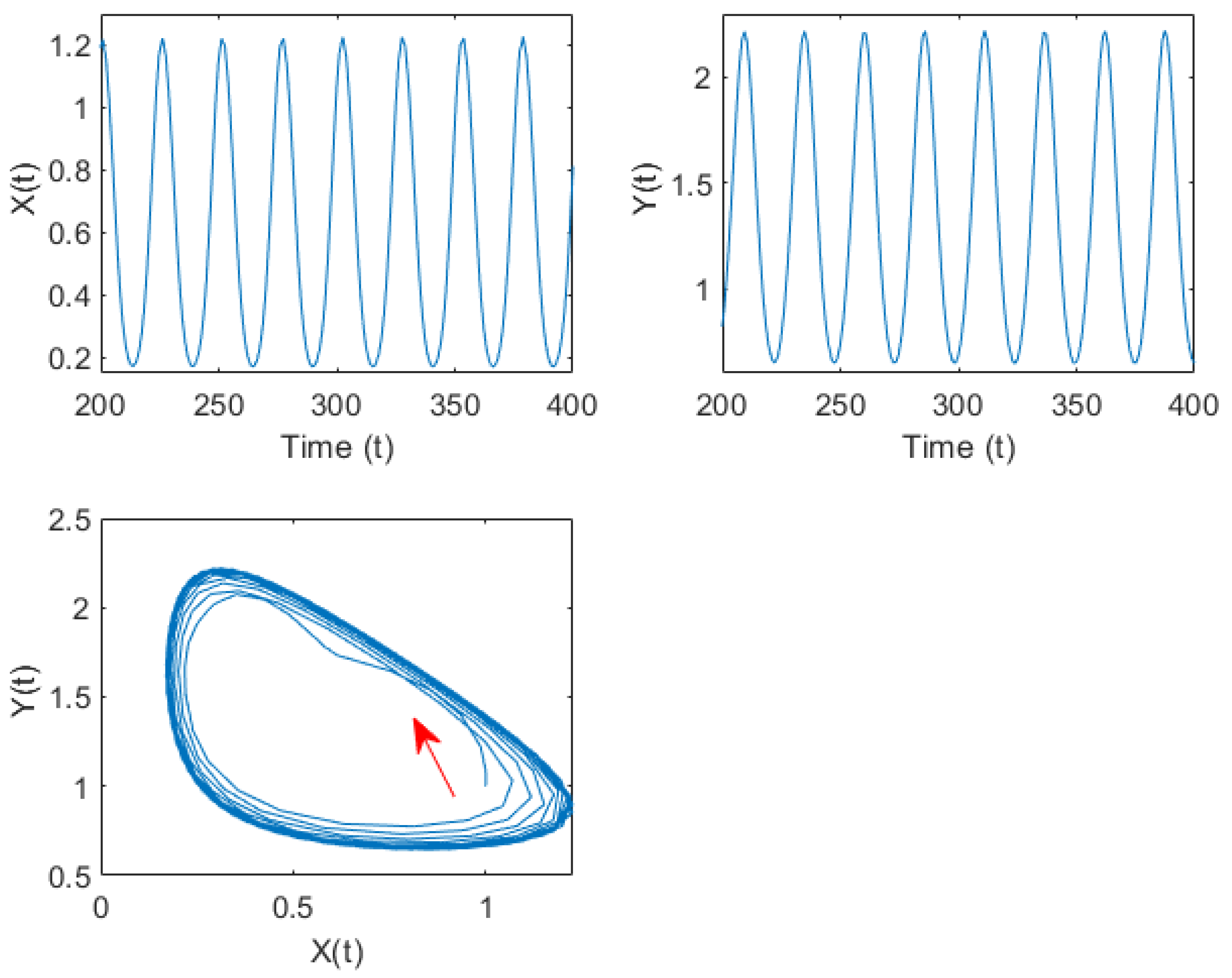
Case 4. ${\tau }_1>0,{\tau }_2=0.$

Select parameters (C), $a=0.7569,\alpha =0.7399,b=0.5541,\beta =0.7393,d=0.6334,r=0.3994,v=0.1737$, and system (6) becomes:

$$\left\{\begin{array}{l}\dot{x}\left(t\right)=x\left(t\right)\left(0.3994-0.7569x\left(t-{\tau }_1\right)-0.5541y\left(t\right)\right),\\ \dot{y}\left(t\right)=0.7399e^{-0.6334{\tau }_2}x\left(t-{\tau }_2\right)y\left(t-{\tau }_2\right)-0.1737y\left(t\right)-0.7393y^2\left(t\right).\end{array}\right.$$

(33)

The internal equilibrium of the system is $E^{\ast }\left(\mathrm{0.4038,0.1692}\right)$, so $\left(H_1\right)$ is valid. After calculation, $\left(H_2\right),\left(H_5\right),\left(H_6\right)$ are true. At this time ${\tau }_1^{\left(0\right)}=4.41$; according to Theorem 5, it can be concluded that, when ${\tau }_1=2<4.41$, the internal equilibrium $E^{\ast }\left(\mathrm{0.4038,0.1692}\right)$ of the system (33) is asymptotically stable, as shown in Figure 7. When ${\tau }_1=5>4.4$, the internal equilibrium $E^{\ast }\left(\mathrm{0.4038,0.1692}\right)$ of the system (33) is unstable. System (33) undergoes Hopf bifurcation at the internal equilibrium $E^{\ast }\left(\mathrm{0.4038,0.1692}\right)$, as shown in Figure 8.

Case 5. ${\tau }_1=0.07,{\tau }_2>0$

Select parameters (D), $a=0.2625,\alpha =0.8945,b=0.3628,\beta =0.0963,d=0.0247,r=0.6433,v=0.3117$, and system (6) becomes:

$$\left\{\begin{array}{l}\dot{x}\left(t\right)=x\left(t\right)\left(0.6433-0.2625x\left(t-{\tau }_1\right)-0.3628y\left(t\right)\right),\\ \dot{y}\left(t\right)=0.8945e^{-0.0247{\tau }_2}x\left(t-{\tau }_2\right)y\left(t-{\tau }_2\right)-0.3117y\left(t\right)-0.0963y^2\left(t\right).\end{array}\right.$$

(34)

Select ${\tau }_1=0.07; {\tau }_1$ belongs to the stable interval, ${\tau }_2$ is the bifurcation parameter, and $\left(H_1\right),\left(H_2\right)$ are true. Figure 9 depicts the curves of $S_0$ and $S_1$ as they change with ${\tau }_2$. It can be seen that $S_0$ intersects with the $x$-axis at two points, which are calculated as follows: ${\tau }_2^{\left(1\right)}=3.17718$ and ${\tau }_2^{\left(2\right)}=15.9877$. According to Theorem 6, when ${\tau }_2=0.5<{\tau }_2^{\left(1\right)}$, the internal equilibrium $E^{\ast }\left(\mathrm{0.5061,1.4069}\right)$ of the system (34) is asymptotically stable, as shown in Figure 10. When ${\tau }_2=3.5>{\tau }_2^{\left(1\right)}$, the internal equilibrium $E^{\ast }\left(\mathrm{0.5420,1.3810}\right)$ of the system (34) is unstable, and Hopf bifurcation occurs from the positive equilibrium $E^{\ast }\left(\mathrm{0.5420,1.3810}\right)$. System (34) undergoes Hopf bifurcation at the internal equilibrium $E^{\ast }\left(\mathrm{0.5420,1.3810}\right)$, as shown in Figure 11.