Article

Erlang-Distributed SEIR Epidemic Models with Cross-Diffusion

by
Victoria Chebotaeva
and
Paula A. Vasquez
*
Department of Mathematics, University of South Carolina, Columbia, SC 29208, USA
*
Author to whom correspondence should be addressed.
Mathematics 2023, 11(9), 2167; https://doi.org/10.3390/math11092167
Submission received: 17 March 2023 / Revised: 25 April 2023 / Accepted: 2 May 2023 / Published: 5 May 2023
(This article belongs to the Special Issue Epidemic Models: Track and Control)

Abstract

:
We explore the effects of cross-diffusion dynamics in epidemiological models. Using reaction–diffusion models of infectious disease, we explicitly consider situations where an individual in a category will move according to the concentration of individuals in other categories. Namely, we model susceptible individuals moving away from infected and infectious individuals. Here, we show that including these cross-diffusion dynamics results in a delay in the onset of an epidemic and an increase in the total number of infectious individuals. This representation provides more realistic spatiotemporal dynamics of the disease classes in an Erlang S E I R model and allows us to study how spatial mobility, due to social behavior, can affect the spread of an epidemic. We found that tailored control measures, such as targeted testing, contact tracing, and isolation of infected individuals, can be more effective in mitigating the spread of infectious diseases while minimizing the negative impact on society and the economy.

1. Introduction

Recent events have made it clear that not only are infectious diseases an inevitable part of our life, but it is also very difficult to predict how an outbreak will evolve or which sectors of a population will be affected the most [1,2,3,4,5,6,7,8]. More relevant to the present study, they have also shown that mathematical models have become important tools needed to understand how diseases spread, to predict future spread dynamics, and, in some sense, to help eliminate some of the uncertainty associated with these diseases. Models not only improve our understanding of the dynamics of the transmission of infections, but they also guide data collection and its interpretation, aid in identifying what drives epidemics, and provide in silico tools used to forecast future directions and to evaluate the potential impact of an intervention [9,10,11,12,13,14,15,16,17,18,19]. It is understood that no model can possibly capture all the intricacies associated with the spread of infectious diseases in a complex social and geographical environment, to quote George Box ‘all models are wrong but some are useful’. Nonetheless, there is a continuing need to evolve existing epidemiological models to include more ‘realistic’ conditions that help advance our understanding of the spatiotemporal evolution of epidemics.
Epidemiological models have been studied for almost 100 years. In 1927, McKendrick and Kermack published the first modern mathematical study that employed epidemiological models [20]. In their formulation, the dynamics of the epidemic process were captured by a coupled system of differential equations, and solutions of the system describe population dynamics in and out of the different groups. In its original form, the Kermack–McKendrick theory divides a population into only two classes, susceptible and infected ( S I ). Years later, it was transformed into a susceptible–infected–recovered ( S I R ) model and, in subsequent works by other authors [21,22,23,24], an exposed (E) class was introduced ( S E I R ). Other modifications have been introduced by adding additional classes to include different disease control measures, such as vaccination, quarantine, and isolation. The resulting models, in general, belong to a family of ODE models which identifies epidemiological states (susceptible, infectious, immune, etc.) and considers constant transition rates between the different classes containing individuals in each disease state. For a comprehensive review of basic epidemic models, the reader is referred to [25].
One of the main assumptions of these S I R / S E I R class of models is that the rate of leaving the exposed or infectious class is constant, regardless of the time spent in that class [26]. This exponential distribution is unrealistic since it is expected that the probability of leaving a given class should depend on the time spent in it. Some studies have shown that the shape of the distribution corresponding to the infectious period has no qualitative effects on the asymptotic values or properties of the system [27,28,29]. However, other studies suggest that the shape of the distribution function greatly affects the persistent likelihood of infections when seasonal variations are considered [10,30,31]. Wearing et al. [26] demonstrated that models with exponential distribution show overoptimistic results that might lead to inadequate levels of control during an epidemic. Consequently, more realistic dynamics are captured if one assumes that the probability of leaving a given class is a function of the time spent within it. In this multi-stage representation, initially, the chance of leaving the E or I classes is small, but this probability increases with time, with upper bounds corresponding to the mean latent or infectious time, respectively. A mathematically convenient way to introduce these dynamics is using Erlang distributions, which can be viewed as gamma distributions with integer shape parameters. Although the Erlang distribution is more restricted in shape than the general gamma distribution, it is sufficiently flexible to provide a good approximation of realistic distributions for latent and infectious periods [29], it is computationally tractable, and it reduces to an exponential distribution when the shape parameter is equal to one.
In this work, we use the so-called “Erlang S E I R model,” shown in Figure 1, which divides the E and I classes into m and n sub-classes, respectively. Since all m latent sub-classes are identical, as are all n infectious sub-classes, we will denote the Erlang S E I R model as S E m I n R .
Champredon et al. [32], showed the equivalency between the S E m I n R model and the renewal equation and formulated analytical expressions for the intrinsic generation-interval distribution that can be used in the renewal equation to give the corresponding epidemic dynamics. Krylova and Earn [29] investigated measles dynamics in NYC. In their study, they used numerical bifurcation analysis to show that the dynamics of SE m I n R models have less effect on the stage duration distribution relative to that of the SI m R models [33]. However, to our knowledge, a study of whether this is the case when other compartments are included has not been carried out. Getz and Dougherty [34] formulated the corresponding discrete, stochastic model for the S E m I n R to capture the inherent randomness in disease transmission. Leontitsis et al. [35], used a susceptible–exposed–asymptomatic–hospitalized–isolated–removed ( S E A H I R ) model to capture SARS-CoV-2 dynamics using data from the United Arab Emirates. In their calculations, the number of stages was kept constant and equal to 5, i.e., S E 5 A 5 H 5 I 5 R .
In addition to temporal dynamics, it is well understood that the spread of an epidemic highly depends on the movement of individuals, and, consequently, including spatial dependence on S E I R models has gathered a lot of attention over the years. Many modeling efforts have been proposed to address several questions arising in this area [12,13,36,37,38,39,40,41,42,43,44,45,46,47,48,49]. A first approximation is to assume individuals’ mobility following a diffusion equation. In their study of a susceptible–infected–susceptible, S I S , reaction–diffusion model, Deng and Wu [42] showed that if the self-diffusion coefficient of the susceptible individuals is equal to the self-diffusion coefficient of the infectious individuals, the disease-free equilibrium is globally attractive if the basic reproductive number is less or equal to one, R 0 1 , while the endemic equilibrium is globally attractive if R 0 > 1 . Wang et al. [49] showed that diseases with larger R 0 tend to spread less compared to those with smaller R 0 . Their studies on the effects of varying diffusion coefficients indicate that diffusion greatly influences the spatiotemporal dynamics in an epidemic model. Allen et al. [38] proposed a spatial S I R reaction–diffusion model and studied the existence, uniqueness, and asymptotic behavior of the endemic equilibrium as the diffusion rate of the susceptible individuals falls to zero in the case where a so-called low-risk sub-habitat is created. Peng [46] continued this research on the impacts of large and small diffusion rates of the susceptible and infectious population on the persistence and extinction of the disease. Their results showed that different strategies for controlling the diffusion rates of individuals might lead to very different spatial distributions of the population. Al-Showaikh et al. also studied the influence of diffusion coefficients in S E I R models [13], using a finite-difference scheme to compute the solution of the spread of measles. Ahmed et al. continued this area of study to investigate the behavior of stability points for measles and other diseases [12,36,37]. Liu [43] presented numerical simulations which prove the global stability of disease-free equilibrium and investigate the dependence of steady-state solutions on the reproductive number, R 0 . Hu and Wang [50] studied a S I R S model with spatiotemporal distribution and population size under both passive diffusion and chemotactic effects captured by cross-diffusion terms. Their results showed that the cross-diffusion terms do not affect the global stability of the corresponding system without cross-diffusion and that an S I R S disease cannot be eradicated by only controlling the diffusive mobility of the susceptible class. Cai et al. [51] investigated the dynamics of a 2D S I model with cross-diffusion dynamics and found that different parameter values lead to different stationary 2D patterns.
Motivated by these previous studies, here we investigate the combined effects of S E n I m R models with the addition of diffusion and cross-diffusion dynamics to simulate spatial reorganization. Phenomenologically speaking, diffusion captures the movement of individuals from regions of high concentration to regions of low concentration. However, if the only effect considered is self-diffusion, individuals move only according to the concentration of individuals in their same class; for instance, susceptible individuals will move away from regions of high concentrations of susceptible individuals but not from regions of high concentration of infectious or exposed individuals. Cross-diffusion, on the other hand, captures the tendency of individuals to move away from high concentrations of individuals in other categories. In practice, studying the effects of cross-diffusion is of interest from a public health perspective since it allows us to investigate a different type of behavior, namely how the movement of susceptible individuals away from regions of high concentration of exposed or infectious individuals affects the evolution of an epidemic. With this in mind, here we use mathematical models and numerical simulations to ask two simple questions: (i) how much does the movement of individuals who have not been infected mitigate or instigate the spread of an infectious disease? And, (ii) what parameters are most susceptible to these spatial dynamics? Additionally, we explore the effects of cross-diffusion in four well-known infectious diseases, SARS, measles, smallpox, and foot-and-mouth. We chose these four cases since their S E m I n R model parameters are available in the literature [1,11,14,52].

2. Model Formulation

2.1. Model Assumptions

  • A given population is divided into four categories, which are functions of both time and space.
    Susceptible ( S ( t , x ) ). Individuals capable of contracting the disease.
    Exposed ( E ( t , x ) ). Infected individuals who are not yet infectious.
    Infectious Symptomatic ( I ( t , x ) ). Individuals capable of transmitting the disease.
    Recovered ( R ( t , x ) ). Individuals from the infectious pool who have recovered.
  • The population size is constant throughout the spatial domain but not at individual points in space,
    N 0 = N ( t ) = Ω S ( t , x ) + i = 1 m E i ( t , x ) + k = 1 n I k ( t , x ) + R ( t , x ) d x , x Ω
  • The disease is not lethal, and birth and death rates are assumed to be equal to μ .
  • The transmission parameter, β , is defined as the average number of effective contacts with other individuals per infectious individual per unit time. An effective contact is an encounter in which the infection is transmitted, we assume this has a probability b. Assuming the contacts per unit time is given by k, the transmission parameter is given by β = k b .
  • The exposed class is divided into m subclasses and m σ is the rate of sequential progression through the subclasses, where 1 / σ is the mean latent period. This is a proxy of modeling the latent period as a gamma distribution with shape parameter m and rate parameter σ , [26].
  • The infectious class is divided into n subclasses and n γ is the rate of sequential progression through the subclasses, where γ is the recovery rate so that 1 / γ is the mean infectious period. As before, this corresponds to a gamma distribution with shape parameter n and rate parameter γ , [26].
  • Recovered individuals are permanently immune.

2.2. System of Equations

The assumptions above lead to the following system of differential equations,
d S ( t ) d t = μ N μ S ( t ) k b I ( t ) S ( t ) N + diffusion terms ,
d E 1 ( t ) d t = μ E 1 ( t ) + k b I ( t ) S ( t ) N m σ E 1 ( t ) + diffusion terms ,
d E i ( t ) d t = μ E i ( t ) + m σ E i 1 ( t ) E i ( t ) + diffusion terms , i = 2 , . . . , m ,
d I 1 ( t ) d t = μ I 1 ( t ) + m σ E m ( t ) n γ I 1 ( t ) ,
d I k ( t ) d t = μ I k ( t ) + n γ I k 1 ( t ) I k ( t ) , k = 2 , . . . , n ,
d R ( t ) d t = μ R ( t ) + n γ I n ,
with the total number of exposed and infectious individuals given by:
E = i = 1 m E i , i = 1 , , m ,
I = k = 1 n I k , k = 1 , , n .
Initially, the population is composed of only susceptible and infectious individuals. Susceptible individuals are distributed uniformly across the spatial domain. Infectious individuals are placed within a band of width two around the center of the spatial domain,
S ( x , 0 ) = S 0 , E ( x , 0 ) = 0 , I ( x , 0 ) = I 0 h ( x ) , R ( x , 0 ) = 0 , L x L ,
where h ( x ) = H x + 1 H x 1 , here H ( · ) is the Heaviside step function.

2.3. Spatial Structure

To the reaction kinetics discussed in the previous section, we add diffusion dynamics,
S ( t , x ) t = Reaction terms + x D S S S ( t , x ) x + x D S E S ( t , x ) x + x D S I S ( t , x ) x ,
E i ( t , x ) t = Reaction terms + x D E E E i ( t , x ) x i = 1 , , m ,
I k ( t , x ) t = Reaction terms + x D I I I k ( t , x ) x k = 1 , , n ,
R ( t , x ) t = Reaction terms + x D R R R ( t , x ) x .
The cross-diffusion coefficient, D a b , determines how restrictive the movement of individuals in class a is with respect to the spatial concentration of individuals in class b. D a b > 0 indicates that a individuals will tend to move away from regions with a large concentration of b individuals.
We impose Neumann boundary conditions in the 1D domain x L , L as,
S ( t , L ) t = E i ( t , L ) t = I k ( t , L ) t = R ( t , L ) t = 0 ,
for i = 1 , , m , k = 1 , , n and t 0 . We note that we keep the domain large enough so that the evolution of the spread is uninfluenced by interactions with the boundary. Investigations of the effects of boundary conditions will be left for future studies.
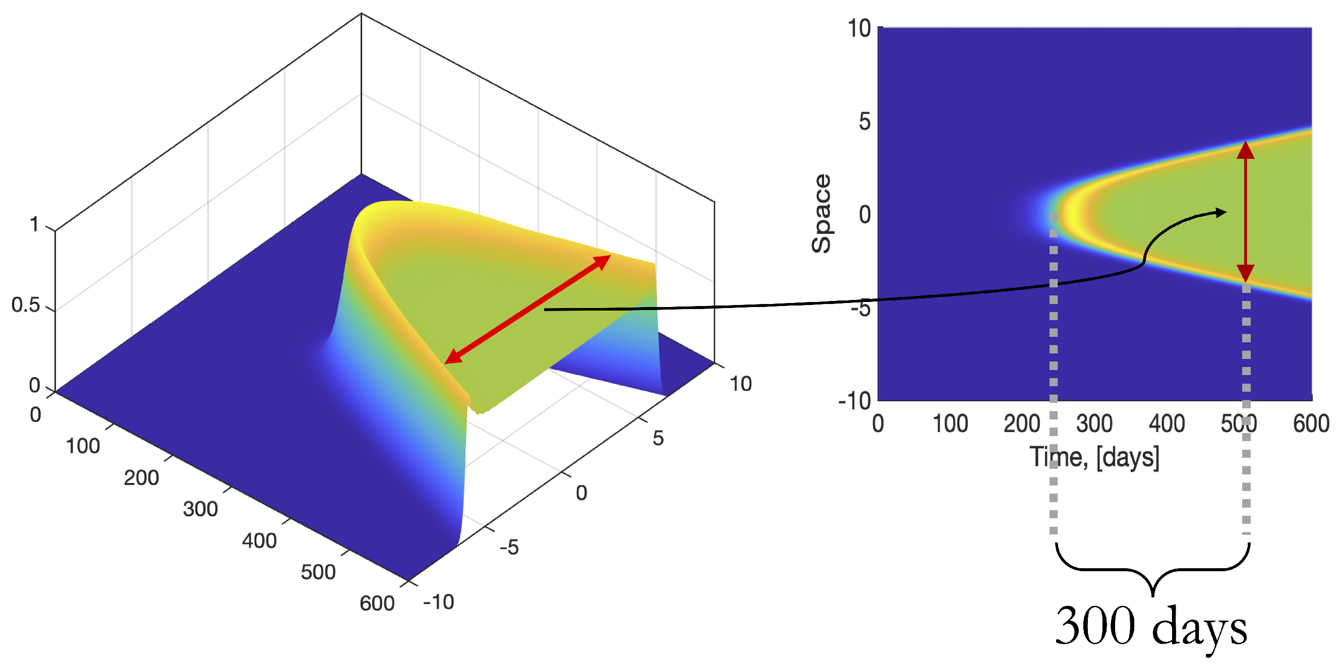
Figure 2 shows a typical three-dimensional view of the distribution of infectious individuals as a function of both time and space, as well as its projection onto the time-space plane. In addition, to compare the effects of different parameters in the evolution dynamics, we introduce a separation metric. This metric captures the spatial separation of the peaks in the number of infectious individuals at a given time, represented by a red arrow in Figure 2. For consistency, we calculate this metric after 300 time steps from the time when the number of infectious individuals, at the middle of the spatial domain, reaches 1% of the total number of individuals.

2.4. Equilibrium Points

It can be shown that the system of Equation (1) has two equilibrium points. A disease-free equilibrium where the only non-zero element is S * = N and an endemic equilibrium,
S * = N R 0 ,
E * = i = 1 m E * i = N 1 m σ m σ + μ m 1 1 R 0 ,
I * = k = 1 n I * k = μ N β R 0 1 ,
R 0 = k b m σ m μ n γ + μ n n γ n n γ + μ n m σ + μ m .
Here R 0 is the corresponding reproductive number and R * = N S * E * I * .
Figure 3 shows the dependence of the equilibrium points on the number of sub-classes within the exposed and infectious classes. Grid planes show the equilibrium solution for m = n = 1 , in this case the system reduces to the well-known S E I R model, whose endemic equilibrium point is found as [37],
S * = N R 0 , E * = μ N μ + σ 1 1 R 0 , I * = μ N β R 0 1 , with R 0 = σ β ( μ + σ ) ( μ + γ ) .
The stability of equilibrium points of epidemic systems is well studied. Li and Wang [53] investigated an S E I R model, Deng and Wu [42] an S I S model, Liu and Li [43] an S E I R model with a linear source, and Yand et al. [54] an S V E I R model with Erlang distributions. All of these studies showed that the endemic equilibrium is globally attractive for cases when the reproductive number is greater than 1, R 0 > 1 , and the disease-free equilibrium is asymptotically stable when the reproductive number is less than 1, R 0 < 1 . We investigated the stability of our system of equations in Appendix A and reached the same conclusions as these authors regarding local stability.
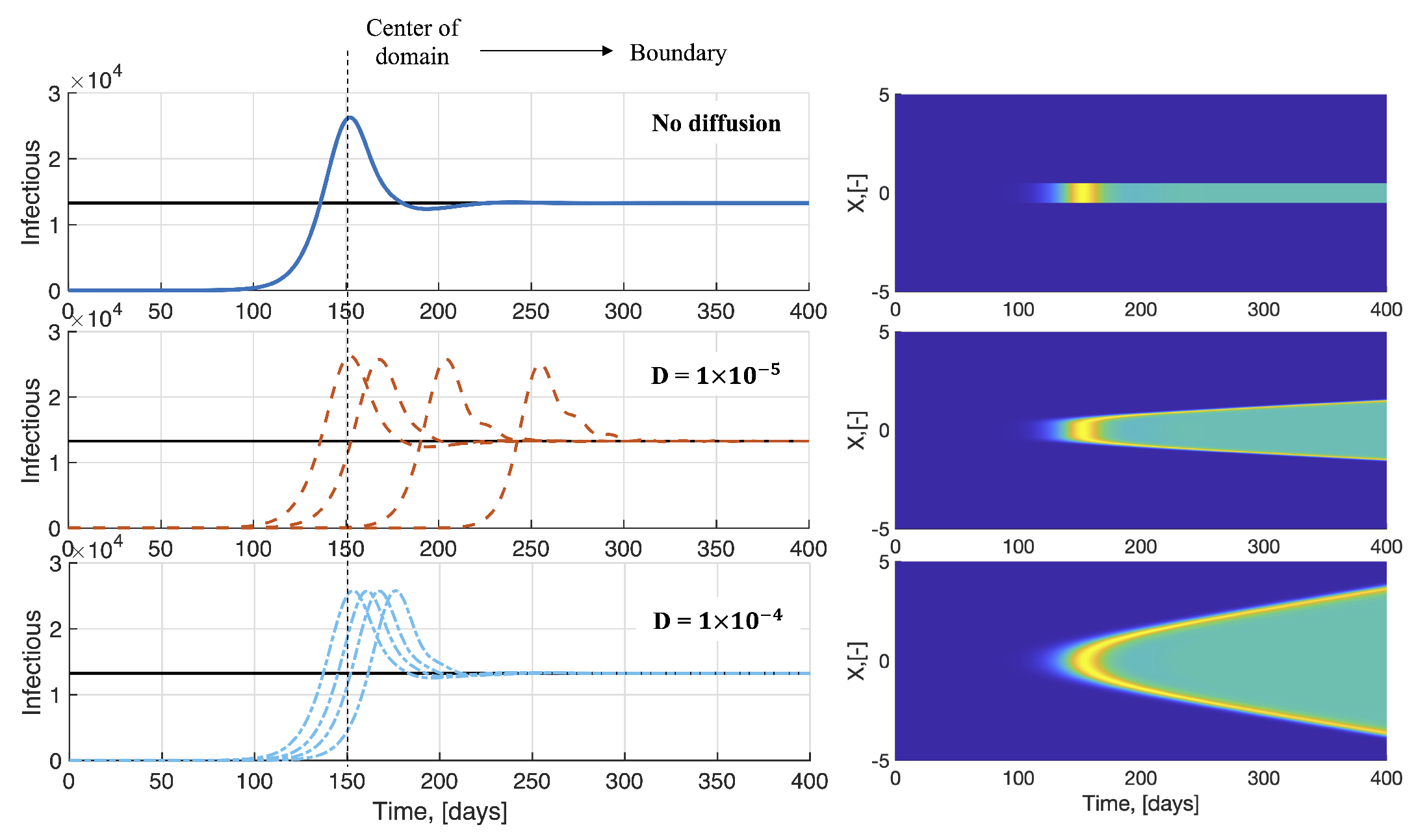
Then, for the system with diffusion and cross-diffusion terms, Equation (4), the equilibrium points, at each location within the spatial domain, are the same as those of the corresponding ordinary differential equation (ODE) system, Equation (1). The only difference between the two systems of equations is the time it takes for a point in space to reach its equilibrium. Figure 4 shows how larger cross-diffusion coefficients decrease the time at which the peak of infection is observed throughout the spatial domain. Since the center of the domain is where, initially, all the infectious individuals are located, Figure 4 shows that there is a dependence on this equilibration time as a function of the distance from the center of the domain.

3. Results and Discussion

As discussed in the introduction, our goal is to investigate the effects of cross-diffusion on epidemic dynamics. In particular, we are interested in discerning the effects of the cross-diffusion coefficients D S E and D S I . That is, we investigate the impact of having susceptible individuals moving away from high concentrations of individuals that have been exposed and might or might not be infectious. For comparison, recall that we use a separation metric defined in Figure 2. In Figure 5, Figure 6 and Figure 7, this metric is plotted in the z-axis as a function of different model parameters.

3.1. Effect of Varying the Transmission Parameter When Cross-Diffusion Is Included

Figure 5 shows how variations of the transmission parameter, β , and the cross-diffusion coefficients will change the evolution of the spatial spread of an epidemic. Regarding the role of cross-diffusion coefficients, we observe a behavior consistent with that shown in Figure 4, where smaller coefficients give rise to less spatial spread. In addition, our results show that the smaller transmissibility also leads to a smaller spatial spread. While transmissibility ( β ) can be controlled by hygienic measures, social distancing, and mask-wearing, mobility ( D S E , D S I ) can be controlled by quarantine and restrictions in traveling. Figure 5 shows that a combination of measures that reduce transmissibility and the mobility of susceptible individuals with respect to infected (but not yet infectious) results in higher control of the spread. While this effect is not as marked when the mobility of susceptible individuals with respect to infectious is increased.

3.2. Effect of Variations in the Average Latent Period When Cross-Diffusion Is Included

Infectious diseases have varying latent (incubation) periods, and this factor plays a crucial role in the spread of the disease. As shown in Figure 6, diseases with shorter latent periods tend to spread more rapidly when combined with higher social mobility.
The latent time is inherent to each disease and, in general, cannot be controlled through approaches aimed at modifying social behavior. However, knowledge of how high or low is the impact of social mobility, given a disease’s latent period, can lead to better decision-making. For instance, Figure 6 shows that for diseases with long latent time, restricting mobility through D S E results in very little changes in the spread of the epidemic, while such restrictive measures might negatively affect the population in other ways. On the other hand, changes in D S I have a significant impact on the spread of the disease. In such cases, imposing strict general lockdown measures that could negatively impact the economy may not be a practical solution, while targeting control will be more efficient.

3.3. Effect of Variations in the Average Infectious Period When Cross-Diffusion Is Included

Infectious diseases also differ in the length of their infectious period. As with the latency period, this is something that cannot be socially controlled. As shown in Figure 7, diseases with longer infectious periods have a smaller impact on a spatial spread from changes in cross-diffusion coefficients.
It is interesting to note that there is a “plateau” region for small to medium values of D S E , with a sudden increase for larger values of the coefficient. This indicates that for diseases with relatively larger infectious periods, very strict lockdowns and traveling measures will not significantly reduce the spread of the disease, while some measures to reduce mobility will definitely make a difference.

3.4. Effect of Varying Erlang Parameters When Cross-Diffusion Is Included

Instead of observing a generic behavior for different values of the Erlang parameters m and n, it makes more physical sense to look at different probability distribution functions (PDFs) resulting from different values of m and n. To do this, we chose four well-studied infectious diseases whose latent and infectious periods had been previously fitted to Erlang distributions and compare their evolution when cross-diffusion is considered. We note that in this section our goal is not to do an in-depth analysis of our four different diseases, SARS, Measles, Smallpox, and Foot-and-mouth disease, but rather use them as tools to aid in the understanding of the role of cross-diffusion. Parameter values for the latent and infectious periods are obtained from [1,11,14,26,52] and given in Table 1, and brief descriptions of each disease are given next; for a more detailed analysis of each of the diseases, the reader is referred to their corresponding references given in Table 1. We analyze the changes in the overall number of infectious individuals and the peak infection both in time and space and correlated these findings to the shape of the corresponding PDFs.

3.4.1. SARS

Severe Acute Respiratory Syndrome (SARS) is a respiratory viral disease, the first case of which was reported in November 2002 in southern China [55]. SARS begins with a fever that usually occurs 2–7 days after infection, but, in some cases, symptoms do not develop for up to 10 days. Chills, headaches, muscle pains, and a general feeling of discomfort often occur. After 2–7 days from the onset of the disease, a dry cough appears. Sometimes SARS progresses to severe pneumonia, leading to respiratory failure and hypoxemia. The patient is most contagious when symptoms develop. It is still unclear whether it is possible to infect other people before the onset of clinical symptoms of the disease or after they have disappeared. The modeling of this disease has been extensively studied, with studies examining its causes, risk factors, and possible treatments [3,18].

3.4.2. Measles

Measles is a viral infection that is easily transmitted and can be expressed as a rash all over the body, accompanied by fever and damage to the mucous membrane of the eyes, mouth, or throat. The disease is transmitted by close proximity to an infectious individual through airborne droplets from talking, coughing, laughing, or sneezing, but it can also spread through an unfiltered ventilation system. The danger of this disease lies in the fact that it can also invade the respiratory tract and the nervous system, or even create problems with the intestinal tract. Most often, children are susceptible to infection because their immune system is not as strong as that of an adult. To this day, this virus can still be found in the population, which can be expressed as an outbreak of infection, but, thanks to vaccination, the disease does not progress as much as before [56]. Through extensive research into the modeling of measles [10,11,12,13,19], scientists have found that prioritizing efforts to prevent and treat the disease can make a meaningful difference in mitigating its effects on populations.

3.4.3. Smallpox

Smallpox is a viral disease that is transmitted between individuals by airborne droplets. It is expressed in the form of purulent rashes throughout the body. Some common symptoms include a feeling of malaise, chills, fever, vomiting, and/or back pain. The rashes resemble ulcers, which often leave scars. This virus enters the human body and then causes viremia [57]. In humans, death is reported in 30% of the cases. This disease is not only found in humans but can also affect animals, such as cows, horses, or monkeys. To eradicate the disease, the decision was made to vaccinate both animals and humans. The investigation of smallpox [1,4,17] modeling in numerous studies has led to a better understanding of how models can be used to inform planning efforts for the disease, especially in light of recent outbreaks of emerging pathogens.

3.4.4. Foot-and-Mouth

Foot-and-mouth disease is a virus most commonly found in livestock. The disease is manifested by a bright rash on the mucous parts of animals. Humans can also become infected by consuming products derived from infected animals. In particular, children are more vulnerable to this disease. An individual who has foot-and-mouth disease feels a strong fever, high temperature, burning in the larynx, redness of the eyes, or strong salivation. The disease is very persistent, resisting frost or dryness, but heating is fatal for the virus [58]. Extensive research has been conducted into the modeling of Foot-and-Mouth disease [14,15,16], with studies assessing a range of factors, including the history and potential duration of epidemics, control strategies, and the broader implications for disease dynamics over time and space.

3.5. Probability Distribution Functions

One convenient way of describing and comparing these diseases is by looking at the probability of being infectious or equivalently by considering the probability density functions for infectious individuals. For Erlang distributions with shape parameter n and scale parameter n γ , the probability density function and corresponding probability are given by,
f ( t , n , n γ ) = ( γ n ) n t n 1 e γ n t ( n 1 ) ! ,
P ( n , t ) = t f ( s , n , n γ ) d s .
Here, P ( n , t ) represents the probability that an individual will be in the n-subclass at time t. Similarly, Equation (8) will give the probability of an exposed individual to remain in the m-subclass, if we replace the shape parameter to m and scale parameter to m σ .
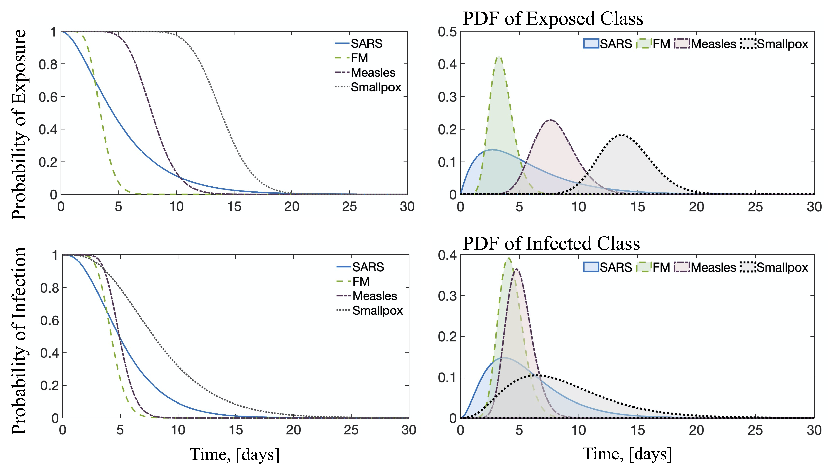
Figure 8 shows the distribution functions and probabilities for the four diseases considered in this study. Smallpox has the longest latent period and this is expressed in the fact that the probability of being exposed remains high for much longer than in other diseases. Similarly, although Measles has the lowest reproductive number, the fact that its latent period is long results in a ‘longer’ probability of being exposed and/or infectious than other diseases with larger R 0 . FM shows a fast peak for both exposure and infection, meaning this is a highly contagious disease but relatively short-lasting. Finally, SARS is not only highly transmittable, given by the R 0 number, but has the ability to ‘linger’ as shown by the temporal evolution of both the probability of exposure and infection.
Further exploration of the data shows that, in measles, there is a big difference in PDFs for exposed and infectious classes as compared to the other three diseases. It does not spread fast in the exposed class, but the transition through the infectious class is fast. In addition, the maximums for both PDFs are very different from each other.
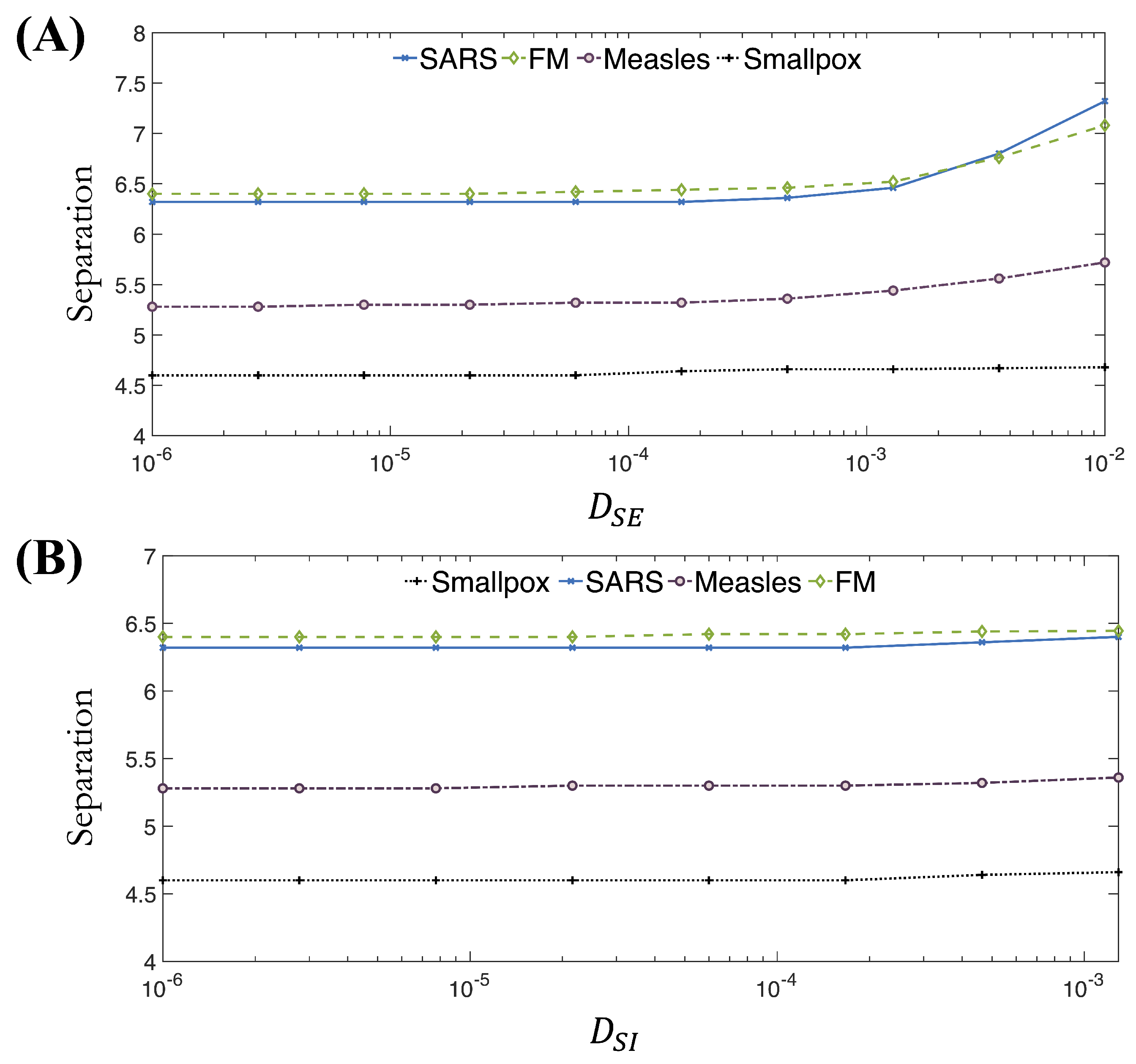
Figure 9 shows the separation metric as a function of D S E and D S I for the four diseases investigated in this section. Using the separation as a metric of spatial spreading, it can be seen that spreading monotonically increases as the cross-diffusion coefficients increase. However, both the magnitude and the rate of the increase vary from disease to disease. Finally, the effect of D S E is stronger than that of D S I .
In terms of separation, a larger magnitude can be translated to a larger number of places within the spatial domain that have reached the endemic equilibrium at a given time. For the four diseases studied, the lower magnitude is that of smallpox, while the highest is for FM. It is clear that smallpox having the smallest magnitude is due to the delay in the first peak, discussed above. On the other hand, the spread of FM corresponds with this disease having the fastest and highest peaks of the PDFs shown in Figure 8. From those distributions, we can conclude that FM is a short-term but very contagious disease. This results in a faster spread in the spatial domain compared to the other diseases, and, as such, we observe a large separation between peaks and more places within the domain reaching endemic equilibrium at a given time.
When the values remain relatively constant, the time scales for spatial spread are comparable to those of the transition from a class to class, so changes in the cross-diffusion coefficient result in minimal changes in the total spreading dynamics. On the other hand, for large cross-diffusion coefficients, the separation starts to increase, meaning that for these large numbers, one can start to see observable differences between the two-time scales.

4. Conclusions

In this study, we explore the spatiotemporal dynamics of S E m I n R models with the addition of cross-diffusion dynamics. Through simulations, we show that controlling the mobility of individuals in the susceptible class alone was insufficient to completely eradicate the spread of the epidemic. In addition, measures to control epidemics based on spatial mobility should be carefully tailored to each disease, since the temporal dynamics specific to each disease greatly affect the evolution of the spatial dynamics. It is understood that the temporal dynamics are controlled by the ODE model parameters (Equation (1)), while spatial dynamics are controlled by the cross-diffusion coefficients (Equation (4)).
Our findings highlight the need for different strategies to control the spread of diseases based on their transmissibility, latent, and infectious periods. This means that when considering measures that restrict mobility, such as quarantine and lockdowns, it is important to recognize that not all measures for epidemic prevention are equally effective for different diseases, and restrictions that are very costly and disrupting should be tailored to each disease to avoid unnecessary collateral damage to the population. By taking into account the specific characteristics of each disease, we can develop more effective approaches to mitigate the spread of infectious diseases while minimizing the impact on society and the economy. For instance, epidemics of diseases with large latent times cannot be efficiently controlled by restrictions in the mobility of non-infected individuals, while such measurements can result in devastating consequences for the general population [5,6,7,8].
It is important to note that our study uses a mathematical model which is not a literal representation of real-life disease spread within the population. For the purpose of modeling, we ignored such factors as traveling, natural growth and decay in population, and contact with individuals outside of the population, among others. Those many factors will definitely affect real-life disease propagation, we expect that future studies will include such assumptions. In addition, future studies might investigate the role of other measures, such as isolation and quarantine, which are more targeted toward individuals in specific infected classes rather than to the population as a whole.

Author Contributions

Conceptualization, P.A.V.; Methodology, V.C. and P.A.V.; Software, V.C. and P.A.V.; Validation, V.C. and P.A.V.; Formal analysis, P.A.V.; Investigation, V.C. and P.A.V.; Resources, P.A.V.; Data curation, P.A.V.; Writing—original draft, V.C. and P.A.V.; Writing—review & editing, V.C. and P.A.V.; Visualization, V.C. and P.A.V.; Supervision, P.A.V.; Project administration, P.A.V.; Funding acquisition, P.A.V. All authors have read and agreed to the published version of the manuscript.

Funding

This research was supported by the DMS Program of the National Science Foundation under CAREER: Multi-Scale Modeling of Biological Gels by Coupling Langevin Equations and Fractional Viscoelastic Constitutive Models, No. 1751339 and Rochester Institute of Technology and University of South Carolina Grant/Cooperative Agreement Number: 80NSSC19K0159 P00004. Any opinions, findings, and conclusions, or recommendations expressed in this material are those of the author(s) and do not necessarily reflect those of the National Science Foundation. Computer simulations were performed using the University of South Carolina’s high-performance computing cluster, Hyperion.

Data Availability Statement

Data is available upon request.

Conflicts of Interest

The authors declare no conflict of interest.

Appendix A. Stability of Equilibrium Points

Appendix A.1. Local Stability

We consider the two equilibrium points of the system, U 0 = N , 0 , 0 , 0 and U 1 = S * , E * , I * , R * , where S * , E * , I * , and R * are given by Equation (6). We use the reproductive number, given in Equation (6d), to evaluate stability and consider our system of the equations in the form,
U ( t ) t + D U ( t ) = F U ( t ) ,
where
D = D S S D S E D S I 0 0 D E E 0 0 0 0 D I I 0 0 0 0 D R R .
Finally, we define A is the Jacobian of F U ( t ) ,
A = μ β I N 0 β S N 0 β I N μ m σ β S N 0 0 m σ μ n γ 0 0 0 n γ μ .
We will use the results from the following two theorems [59],
Theorem A1.
For the linearized system
z t = D Δ z + A z ,
Let 0 = λ 0 < λ 1 λ 2 λ 3 , be the sequence of eigenvalues of the operator Δ subject to the homogeneous Neumann conditions, then
  • The zero solution is globally asymptotically stable if for each non-negative integer n the eigenvalue of A λ n D have negative real parts. Further, there exists positive constants K, ω such that for any t > 0 ,
    | | z ( t , x ) | | K e ω t | | α ( x ) | | .
  • The zero solution is stable if for each non-negative integer n the eigenvalues of A λ n D have non-positive real parts and those with zero real parts have simple elementary divisors.
  • The zero solution is unstable if for some n there exists an eigenvalue of A λ n D with either positive real part or zero real part with a non-simple elementary divisor.
Theorem A2.
The zero solution of z t = D Δ z + f ( z ) , is asymptotically stable if the zero solution of the linearized problem (A1) is asymptotically stable.
Theorem A3.
If R 0 < 1 , the disease-free equilibrium point U 0 is asymptotically stable.
Proof. 
Let A = D F U 0 . By Theorems A1 and A2 the equilibrium point U 0 is asymptotically stable if for each non-negative integer i the eigenvalue of matrix A ξ i D have a negative real part.
Let P 0 = A ( N , 0 , 0 , 0 ) ξ i D λ I
P 0 = μ ξ i D S S λ ξ i D S E β ξ i D S I 0 0 μ m σ ξ i D E E λ β 0 0 m σ μ n γ ξ i D I I λ 0 0 0 n γ μ m σ ξ i D R R λ .
d e t P 0 = μ ξ i D R R λ μ ξ i D S S λ p 2 ( λ ) ,
where
p ( λ ) = λ 2 + 2 μ + m σ + n γ + ξ i D E E + D I I λ + μ + m σ + ξ i D E E μ + n γ + ξ i D I I m β σ .
This gives the eigenvalues,
λ 1 = μ ξ i D R R 0 λ 2 = μ ξ i D S S 0 λ 3 , 4 = 2 μ + m σ + n γ + ξ i D E E + D I I ± ( D I I D E E ) ξ m σ + n γ 2 + 4 m σ β 2 .
Since 2 μ + m σ + n γ + ξ i D E E + D I I 0 , the real parts of all the eigenvalues are negative and N , 0 , 0 , 0 is asymptotically stable. □
Theorem A4.
If R 0 > 1 , the endemic equilibrium point U 1 is asymptotically stable.
Proof. 
Let P 1 = A S * , E * , I * , R * ξ i D λ I
P 1 = μ β I * N ξ i D S S λ ξ D S E β S * N ξ D S I 0 β I * N μ m σ ξ i D E E λ β S * N 0 0 m σ μ n γ ξ i D I I λ 0 0 0 n γ μ ξ i D R R λ = μ R 0 ξ i D S S λ ξ i D S E β / R 0 ξ D S I 0 μ ( R 0 1 ) μ m σ ξ i D E E λ β / R 0 0 0 m σ μ n γ ξ i D I I λ 0 0 0 n γ μ ξ i D R R λ
d e t P 1 = μ + ξ i D R R + λ λ 3 + a 2 λ 2 + a 1 λ + a 0 ,
where
a 0 = D S S D E E μ + n γ + D S S D I I μ + m σ + μ D I I D E E R 0 + D S E ( R 0 1 ) ξ i 2 + μ D S E R 0 1 μ + n γ D S S μ + m σ μ + n γ + μ R 0 D I I μ + m σ + D E E μ + n γ ξ i + μ R 0 μ + m σ μ + n γ m σ β R 0 μ R 0 + ξ i D S S , a 1 = D S S D E E + D S S D I I + D E E D I I ξ i 2 + n γ D S S + D E E + m σ D S S + D I I + μ R 0 1 D S I + μ 2 D S S + R 0 1 D S E + D E E + D I I ( 1 + R 0 ) ξ i + ( 1 + 2 R 0 ) μ 2 + m σ + n γ ( 1 + R 0 ) μ + m σ n γ β R 0 , a 2 = m σ + n γ + μ ( 2 + R 0 ) + ξ i D S S + D E E + D I I .
By the Routh–Hurwitz criterion λ 3 + a 2 λ 2 + a 1 λ + a 0 = 0 have roots with negative real parts if a 0 , a 1 , a 2 > 0 , and a 1 a 2 > a 0 . Since R 0 > 1 , the real parts of all the eigenvalues are negative and S * , E * , I * , R * is asymptotically stable.
When m , n > 1 the stability of the equilibrium points cannot be determined analytically. We calculated the eigenvalues for the four cases we investigate in this paper and their real parts are plotted in Figure A1.
Figure A1. The real part of the eigenvalues for P 1 using parameter values from Table 1 corresponding to the four cases explored in this study.
Mathematics 11 02167 g0a1
 □

References

  1. Koplan, J.P.; Azizullah, M.F.S. Urban hospital and rural village smallpox in Bangladesh. Trop. Georg. Med. 1978, 30, 355–358. [Google Scholar]
  2. Daszak, P.; Cunningham, A.A.; Hyatt, A.D. Emerging Infectious Diseases of Wildlife—Threats to Biodiversity and Human Health. Science 2000, 287, 443–449. [Google Scholar] [CrossRef] [PubMed]
  3. Donnelly, C.A.; Ghani, A.C.; Leung, G.M.; Hedley, A.J.; Fraser, C.; Riley, S.; Abu-Raddad, L.J.; Ho, L.M.; Thach, T.Q.; Chau, P.; et al. Epidemiological determinants of spread of causal agent of severe acute respiratory syndrome in Hong Kong. Lancet 2003, 361, 1761–1766. [Google Scholar] [CrossRef]
  4. Gani, R.L.S. Transmission potential of smallpox in contemporary populations. Nature 2001, 414, 748–751. [Google Scholar] [CrossRef] [PubMed]
  5. Holmes, E.A.; O’Connor, R.C.; Perry, V.H.; Tracey, I.; Wessely, S.; Arseneault, L.; Ballard, C.; Christensen, H.; Silver, R.C.; Everall, I.; et al. Multidisciplinary research priorities for the COVID-19 pandemic: A call for action for mental health science. Lancet Psychiatry 2020, 7, 547–560. [Google Scholar] [CrossRef] [PubMed]
  6. Nicola, M.; Alsafi, Z.; Sohrabi, C.; Kerwan, A.; Al-Jabir, A.; Iosifidis, C.; Agha, M.; Agha, R. The socio-economic implications of the coronavirus pandemic (COVID-19): A review. Int. J. Surg. 2020, 78, 185–193. [Google Scholar] [CrossRef] [PubMed]
  7. Chinazzi, M.; Davis, J.T.; Ajelli, M.; Gioannini, C.; Litvinova, M.; Merler, S.; Pastore y Piontti, A.; Mu, K.; Rossi, L.; Sun, K.; et al. The effect of travel restrictions on the spread of the 2019 novel coronavirus (COVID-19) outbreak. Science 2020, 368, 395–400. [Google Scholar] [CrossRef]
  8. Kraemer, M.U.; Yang, C.H.; Gutierrez, B.; Wu, C.H.; Klein, B.; Pigott, D.M.; Open COVID-19 Data Working Group; Louis du Plessis 5; Du Plessis, L.; Faria, N.R.; et al. The effect of human mobility and control measures on the COVID-19 epidemic in China. Science 2020, 368, 493–497. [Google Scholar] [CrossRef]
  9. Keeling, M.J.; Rohani, P. Modeling Infectious Diseases in Humans and Animals; Princeton University Press: Princeton, NJ, USA, 2011. [Google Scholar]
  10. Keeling, M.J.; Grenfell, B.T. Disease extinction and community size: Modeling the persistence of measles. Science 1997, 275, 65–67. [Google Scholar] [CrossRef]
  11. Simpson, R.E.H. Infectiousness of communicable diseases in the household (measles, chickenpox, and mumps). Lancet 1952, 263, 549–554. [Google Scholar]
  12. Nauman, A.; Rafiq, M.; Rehman, M.; Ali, M.; Ahmad, M. Numerical modeling of SEIR measles dynamics with diffusion. Commun. Math. Appl. 2018, 9, 315. [Google Scholar]
  13. Al-Showaikh, F.N.M.; Twizell, T.E. One-dimensional measles dynamics. Appl. Math. Comput. 2004, 152, 169–194. [Google Scholar] [CrossRef]
  14. Ferguson, N.M.; Donnelly, C.A.; Anderson, R.M. The foot-and-mouth epidemic in Great Britain: Pattern of spread and impact of interventions. Science 2001, 292, 1155–1160. [Google Scholar] [CrossRef] [PubMed]
  15. Woolhouse, M.; Chase-Topping, M.; Haydon, D.; Friar, J.; Matthews, L.; Hughes, G.; Shaw, D.; Wilesmith, J.; Donaldson, A.; Cornell, S.; et al. Foot-and-mouth disease under control in the UK. Nature 2001, 411, 258–259. [Google Scholar] [CrossRef]
  16. Keeling, M.J.; Woolhouse, M.E.; Shaw, D.J.; Matthews, L.; Chase-Topping, M.; Haydon, D.T.; Cornell, S.J.; Kappey, J.; Wilesmith, J.; Grenfell, B.T. Dynamics of the 2001 UK foot and mouth epidemic: Stochastic dispersal in a heterogeneous landscape. Science 2001, 294, 813–817. [Google Scholar] [CrossRef]
  17. Ferguson, N.M.; Keeling, M.J.; John Edmunds, W.; Gani, R.; Grenfell, B.T.; Anderson, R.M.; Leach, S. Planning for smallpox outbreaks. Nature 2003, 425, 681–685. [Google Scholar] [CrossRef]
  18. Lipsitch, M.; Cohen, T.; Cooper, B.; Robins, J.M.; Ma, S.; James, L.; Gopalakrishna, G.; Chew, S.K.; Tan, C.C.; Samore, M.H.; et al. Transmission dynamics and control of severe acute respiratory syndrome. Science 2003, 300, 1966–1970. [Google Scholar] [CrossRef]
  19. Bakare, E.; Adekunle, Y.; Kadiri, K. Modelling and simulation of the dynamics of the transmission of measles. Int. J. Comput. Trends Technol. 2012, 3, 174–178. [Google Scholar]
  20. Kermack, W.O.; McKendrick, A.G. A contribution to the mathematical theory of epidemics. Proc. R. Soc. A 1927, 115, 700–721. [Google Scholar]
  21. Cooke, K.L. Stability analysis for a vector disease model. Rocky Mt. J. Math. 1979, 9, 31–42. [Google Scholar] [CrossRef]
  22. Hethcote, H.W.; Van den Driessche, P. Some epidemiological models with nonlinear incidence. J. Math. Biol. 1991, 29, 271–287. [Google Scholar] [CrossRef] [PubMed]
  23. Diekmann, O.; Heesterbeek, J.A.P. Mathematical Epidemiology of Infectious Diseases: Model Building, Analysis and Interpretation; John Wiley & Sons: Hoboken, NJ, USA, 2000; Volume 5. [Google Scholar]
  24. Bratus, S.A.; Novozhilov, A.S.; Platonov, A. Dynamical Systems and Models in Biology; Fizmatlit: Moscow, Russia, 2010. [Google Scholar]
  25. Hethcote, H.W. The mathematics of infectious diseases. SIAM Rev. 2000, 42, 599–653. [Google Scholar] [CrossRef]
  26. Wearing, H.J.; Rohani, P.; Keeling, M.J. Appropriate models for the management of infectious diseases. PLoS Med. 2005, 2, e174. [Google Scholar] [CrossRef] [PubMed]
  27. Blythe, S.; Anderson, R. Distributed incubation and infectious periods in models of the transmission dynamics of the human immunodeficiency virus (HIV). Math. Med. Biol. 1988, 5, 1–19. [Google Scholar] [CrossRef] [PubMed]
  28. Hethcote, H.W.; Tudor, D.W. Integral equation models for endemic infectious diseases. J. Math. Biol. 1980, 9, 37–47. [Google Scholar] [CrossRef] [PubMed]
  29. Krylova, O.; Earn, D.J. Effects of the infectious period distribution on predicted transitions in childhood disease dynamics. J. R. Soc. Interface 2013, 10, 20130098. [Google Scholar] [CrossRef]
  30. Lloyd, A.L. Realistic distributions of infectious periods in epidemic models: Changing patterns of persistence and dynamics. Theor. Popul. Biol. 2001, 60, 59–71. [Google Scholar] [CrossRef]
  31. Lloyd, A.L. Destabilization of epidemic models with the inclusion of realistic distributions of infectious periods. Proc. R. Soc. London Ser. B 2001, 268, 985–993. [Google Scholar] [CrossRef]
  32. Champredon, D.; Dushoff, J.; Earn, D.J. Equivalence of the Erlang-distributed SEIR epidemic model and the renewal equation. SIAM J. Appl. Math. 2018, 78, 3258–3278. [Google Scholar] [CrossRef]
  33. Zhu, H.; Li, Y.; Jin, X.; Huang, J.; Liu, X.; Qian, Y.; Tan, J. Transmission dynamics and control methodology of COVID-19: A modeling study. Appl. Math. Model. 2021, 89, 1983–1998. [Google Scholar] [CrossRef]
  34. Wayne, M.; Getz, E.R.D. Discrete stochastic analogs of Erlang epidemic models. J. Biol. Dyn. 2018, 12, 16–38. [Google Scholar]
  35. Leontitsis, A.; Senok, A.; Alsheikh-Ali, A.; Al Nasser, Y.; Loney, T.; Alshamsi, A. Seahir: A specialized compartmental model for COVID-19. Int. J. Environ. Res. Public Health 2021, 18, 2667. [Google Scholar] [CrossRef] [PubMed]
  36. Ahmed, N.; Elsonbaty, A.; Raza, A.; Rafiq, M.; Adel, W. Numerical simulation and stability analysis of a novel reaction—Diffusion COVID-19 model. Nonlinear Dyn. 2021, 106, 1293–1310. [Google Scholar] [CrossRef] [PubMed]
  37. Ahmed, N.; Tahira, S.; Rafiq, M.; Rehman, M.; Ali, M.; Ahmad, M. Positivity preserving operator splitting nonstandard finite difference methods for SEIR reaction diffusion model. Open Math. 2019, 17, 313–330. [Google Scholar] [CrossRef]
  38. Allen, L.J.; Bolker, B.M.; Lou, Y.; Nevai, A.L. Asymptotic profiles of the steady states for an SIS epidemic reaction-diffusion model. Discret. Contin. Dyn. Syst.-A 2008, 21, 1. [Google Scholar] [CrossRef]
  39. Bendahmane, M.; Langlais, M. A reaction-diffusion system with cross-diffusion modeling the spread of an epidemic disease. J. Evol. Eq. 2010, 10, 883–904. [Google Scholar] [CrossRef]
  40. Capasso, V.; Di Liddo, A. Asymptotic behaviour of reaction-diffusion systems in population and epidemic models. J. Math. Biol. 1994, 32, 453–463. [Google Scholar] [CrossRef]
  41. Capasso, V. Mathematical Structures of Epidemic Systems; Springer Science & Business Media: Berlin/Heidelberg, Germany, 2008; Volume 97. [Google Scholar]
  42. Deng, K.; Wu, Y. Dynamics of a susceptible-infected-susceptible epidemic reaction-diffusion model. Proc. R. Soc. Edinb. Sect. A 2016, 146, 929. [Google Scholar] [CrossRef]
  43. Liu, P.; Li, H.X. Global behavior of a multi-group SEIR epidemic model with age structure and spatial diffusion. Math. Biosci. Eng. 2020, 17. [Google Scholar] [CrossRef]
  44. Milner, F.A.; Zhao, R. SIR model with directed spatial diffusion. Math. Popul. Stud. 2008, 15, 160–181. [Google Scholar] [CrossRef]
  45. Mulone, G.; Straughan, B.; Wang, W. Stability of epidemic models with evolution. Stud. Appl. Math. 2007, 118, 117–132. [Google Scholar] [CrossRef]
  46. Peng, R. Asymptotic profiles of the positive steady state for an SIS epidemic reaction–diffusion model. Part I. J. Differ. Equ. 2009, 247, 1096–1119. [Google Scholar] [CrossRef]
  47. Reluga, T. A two-phase epidemic driven by diffusion. J. Theor. Biol. 2004, 229, 249–261. [Google Scholar] [CrossRef]
  48. Wang, B.G.; Li, W.T.; Wang, Z.C. A reaction–diffusion SIS epidemic model in an almost periodic environment. Z. Angew. Math. Phys. 2015, 66, 3085–3108. [Google Scholar] [CrossRef]
  49. Wang, W.; Cai, Y.; Wu, M.; Wang, K.; Li, Z. Complex dynamics of a reaction–diffusion epidemic model. Nonlinear Anal. 2012, 13, 2240–2258. [Google Scholar] [CrossRef]
  50. Hu, Y.; Wang, J. Dynamics of an SIRS epidemic model with cross-diffusion. Commun. Pure Appl. Anakysis 2022, 21. [Google Scholar] [CrossRef]
  51. Cai, Y.; Chi, D.; Liu, W.; Wang, W. Stationary patterns of a cross-diffusion epidemic model. Abstr. Appl. Anal. 2013, 2013, 852698. [Google Scholar] [CrossRef]
  52. Riley, S.; Fraser, C.; Donnelly, C.A.; Ghani, A.C.; Abu-Raddad, L.J.; Hedley, A.J.; Leung, G.M.; Ho, L.M.; Lam, T.H.; Thach, T.Q.; et al. Transmission dynamics of the etiological agent of SARS in Hong Kong: Impact of public health interventions. Science 2003, 300, 1961–1966. [Google Scholar] [CrossRef]
  53. Li, M.; Wang, L. Global Stability in some SEIR epidemic models. In Mathematical Approaches for Emerging and Reemerging Infectious Diseases; Springer: Berlin/Heidelberg, Germany, 2002; Volume 126, pp. 295–311. [Google Scholar]
  54. Duan, X.; Yuan, S.; Qiu, Z.; Ma, J. Global stability of an SVEIR epidemic model with ages of vaccination and latency. Comput. Math. Appl. 2014, 68, 288–308. [Google Scholar] [CrossRef]
  55. Available online: https://www.cdc.gov/sars/ (accessed on 6 December 2017).
  56. Available online: https://www.cdc.gov/measles/ (accessed on 5 November 2020).
  57. Available online: https://www.cdc.gov/smallpox/ (accessed on 12 July 2017).
  58. Available online: https://www.cdc.gov/hand-foot-mouth/ (accessed on 2 February 2021).
  59. dos Santos, J.P.C.; Monteiro, E.; Ferreira, J.C.; Teixeira Lemes, N.H.; Rodrigues, D.S. Well Posedness and Qualitative Analysis of a SEIR Model with Spatial Diffusion for COVID-19 Spread. 2022. Available online: https://ssrn.com/abstract=4208624 (accessed on 3 May 2023).
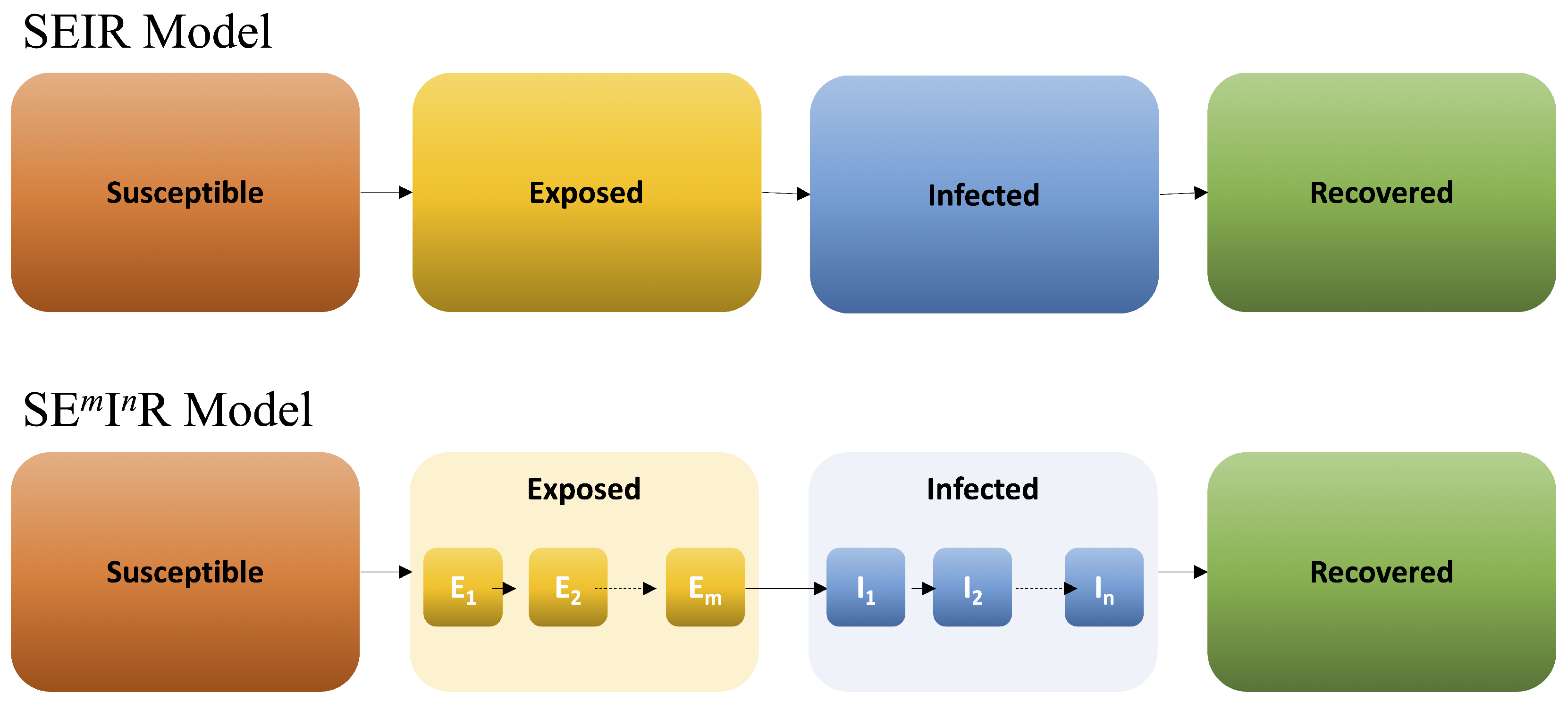
Figure 1. In the S E I R model the population is divided into 4 compartments, Susceptible, Exposed, Infected, and Recovered. In the S E m I n R model, the transition probabilities are made more realistic by subdividing the E and I compartments into m and n sub-compartments, respectively. In this way, individuals in the E 1 sub-compartment have a smaller probability than individuals in the E m sub-compartment to move to the I class.
Mathematics 11 02167 g001
Figure 2. (Left) 3D plot of normalized number of infectious individuals. (Right) Projection onto the time-space plane of the plot on the left. Red arrows show the separation between peaks after 300 time steps after the number of infectious starts rising. The length of the red arrow defines our separation metric, which will be used to compare different behaviors in the Results section.
Mathematics 11 02167 g002
Figure 3. Equilibrium points for the S E m I n R as functions of n and m. Planes indicate the theoretical equilibrium points for the S E I R model (Equation (7)); numerically, these values should correspond to m = 1 , n = 1 , marked by a red x in the plots.
Mathematics 11 02167 g003
Figure 4. Equilibrium points for the S E m I n R model. At the center of the domain, the evolution of the system remains the same with or without cross-diffusion; other points within the domain will change their behavior according to the cross-diffusion dynamics imposed on the system. The higher the cross-diffusion coefficient, the faster all points in the domain will reach the steady state. Black lines mark the corresponding theoretical equilibrium given by Equation (6).
Mathematics 11 02167 g004
Figure 5. (Left) Effects of changing the cross-diffusion coefficient between susceptible and exposed D S E and the transmission parameter β on the change in separation. (Right) Effects of changing the cross-diffusion coefficient between susceptible and infectious D S I and the transmission parameter β on the change in separation. Lower β and D S # result in a reduced spatial spread: the separation between peaks is the smallest (blue regions), while large cross-diffusion coefficients and transmission parameters result in a larger spread (yellow regions).
Mathematics 11 02167 g005
Figure 6. (Left): Effects of changing cross-diffusion coefficient D S E and latent time T e on the spatial spread of an epidemic. (Right): Effects of changing cross-diffusion coefficient D S I and latent time T e on the disease spread. Lower separation corresponds to lower spread (blue regions), and higher separation to higher spread (yellow regions).
Mathematics 11 02167 g006
Figure 7. (Left): Effects of changing cross = diffusion coefficient D S E and infectious time T i on the change in separation. (Right): Effects of changing cross-diffusion coefficient D S I and infectious time T i on the change in separation. Lower separation corresponds to lower spread (blue regions), and higher separation to higher spread (yellow regions).
Mathematics 11 02167 g007
Figure 8. The change in the probability of remaining exposed and infectious as a function of time for all 4 diseases and their corresponding probability density functions. Equations given by Equation (8) and parameters in Table 1.
Mathematics 11 02167 g008
Figure 9. Separation for varying values of the cross-diffusion coefficients (A) D S E and (B) D S I . These coefficients capture the movement of susceptible individuals away from high concentrations of infected and infectious individuals, respectively. The larger the coefficient the faster individuals move away from the regions of high concentrations.
Mathematics 11 02167 g009
Table 1. Model parameters for each of the four diseases considered in this study. Other model parameters are, μ = 0.05 , b = 0.3, k = 10 , and β = 3 . R 0 values are found using Equation (6d).
DiseasemnLatent Period 1 / σ , (Days)Infectious Period 1 / γ , (Days) R 0 Reference
Measles2020858.88[11]
Foot-and-Mouth13173.54.39.7[14]
SARS235.365.510.79[52]
smallpox404148.610.05[1]
Disclaimer/Publisher’s Note: The statements, opinions and data contained in all publications are solely those of the individual author(s) and contributor(s) and not of MDPI and/or the editor(s). MDPI and/or the editor(s) disclaim responsibility for any injury to people or property resulting from any ideas, methods, instructions or products referred to in the content.