The Regulator Problem to the Convection–Diffusion Equation

Abstract

In this paper, from linear operator, semigroup and Sturm–Liouville problem theories, an abstract system model for the convection–diffusion (C–D) equation is proposed. The state operator for this abstract system model is here defined as given in the form of the Sturm–Liouville differential operator (SLDO) plus an integral term of the same SLDO. Our aim is to achieve the trajectory tracking task in the presence of external disturbances to the C–D equation invoking the regulator problem theory, where the state from a finite-dimensional exosystem is the state to the feedback law. In this context, the regulator (Francis) equations, established from the abstract system model for the C–D equation, here are solved; i.e., the state feedback regulator problem (SFRP) for the C–D system has a solution. Our proposal is validated via numerical simulation results.

1. Introduction

Systems whose dynamics evolve in an infinite-dimensional Hilbert space are denominated as infinite-dimensional systems modeled by partial differential equations (PDEs), which are also termed as distributed parameter systems (DPSs), since it reflects the spatial distribution of a physical quantity. The main goal when designing the control system for these class of systems is satisfying stability in the presence of external disturbances.

Dynamical systems given either in the input–output equation form, modeled through ordinary differential equations (ODEs), or in the state-space form can be transformed to the transfer function (transfer matrix) form; this latter description is always rational with real coefficients. Transfer functions from DPSs are non-rational functions which can be analytic in the complex plane and having no poles, such as in the case of the transport equation, namely, a first-order PDE, or having only zeros in their denominator, such as for the diffusion equation with Neumann boundary conditions or for the wave equation [1]. From classical control theory, classical controllers are designed from the knowledge of the transfer function, i.e., from an output/input description of the system. From DPSs, if a closed-form expression of their transfer function is provided, then the direct design of the controller may be possible. This approach is referred to as direct controller design. The primary drawback from this approach is the requirement of an explicit representation of the transfer function. In addition, the controller design will be infinite-dimensional, so this must be approximated by a finite-dimensional system. For some practical applications, when a transfer function for a DPS is not available, then the indirect controller design approach is the most common alternative to be employed. It consists of obtaining a finite-dimensional approximation of the system from which the controller can be designed [2].

The design of a feedback law such that it guarantees the tracking of a reference signal in the presence of an external disturbance, the latter generated through an exosystem, is the main objective when invoking the regulator problem theory [3]. Beyond finite-dimensional systems, the regulator problem theory has been playing an interesting role in the control of infinite-dimensional systems. In this work, we deal with the state feedback regulator problem (SFRP) where the state of the feedback law is from a finite-dimensional exosystem.

From linear finite-dimensional systems, the regulator problem theory has been extended to infinite-dimensional systems also known as DPSs [4,5,6,7,8]. In [6,7], control systems governed by a discrete spectral operator were introduced, where the so-called state operator meets with the property of spectrum decomposition [9,10] from which a controllability condition was determined implying the stabilizability of the control system through a finite-dimensional controller. In [8], the regulator problem was extended to DPSs for bounded input and output operators, with reference and disturbance signals generated through a finite-dimensional exosystem, providing criteria for the solvability of the regulator equations. The linear regulator problem when considering bounded input and output operators but also bounded disturbance operators entering along the entire interval is shown in [11]. In this last work, the linear regulation problem was solved to the heat equation, damped wave equation, harmonic tracking for a coupled wave equation, control of a damped Rayleigh beam, vibration of a 2D plate, thermal control of a 2D fluid flow, thermal regulation in a 3D room, and control of a linearized Stokes flow in 2D. Reviews about the generalization of the regulator problem to infinite-dimensional systems can be found in [12,13]. The output regulation problem for DPSs has been studied extensively for different classes of PDEs systems; a summary is given in [14]. In [14,15], following the methodology from [11] which is based on the derivation of the transfer function from the system model representation in the state-space form to the solvability of the regulator equations, the SFRP was solved for the R–D equation. An abstract model for the R–D equation was derived where the state operator has the form given by the Sturm–Liouville differential operator (SLDO) plus a parametric term. Simulation results validate their proposal showing the achievement of the regulation tasks to a set-point as well as to harmonic tracking under both set-point disturbance and harmonic disturbance rejection.

The phenomena described by a C–D equation exhibit diffusion and convection properties that are common in many scenarios. Diffusion is the mix of a substance through the medium while convection is the movement of the substance by means of the medium, e.g., when considering smoke rising from a chimney, the smoke particles are convected upward with the air and diffuse within the air currents. It is possible for the convection of the substance to contribute more of a movement in the substance than the diffusion itself. In [16], an illustration about the solutions and behavior for diffusion problems when including the convection term is given. A review of different diffusion models, namely, the Maxwell–Stefan model, the generalized Fick’s law, the classical Fick’s law, and the irreversible thermodynamic model, is given in [17]. The importance for an accurate measuring and prediction of the diffusion coefficients as well as the importance of considering the dragging effect is emphasized. So, an accurate method to approximate the gas–oil mass transfer mechanism based on irreversible thermodynamics was proposed. In this last work, molecular diffusion is only discussed since the system was assumed to be an isothermal one. His proposal is validated through numerical examples and experimental test cases when considering convection for some cases. A chemotaxis–diffusion–convection coupling system which describes a form of buoyant convection in which the fluid develops convection cells and plume patterns is studied in [18]. The pattern formation and hydrodynamical stability of the system was investigated through the development of an upwind finite element method based on a two-dimensional convective chemotaxis–fluid model. Numerical results show the influence of the deterministic initial condition on the overall behavior regarding the number of plumes and that the overall system was stabilized by the chemotaxis. To the best of our knowledge, there is no work about the solvability of the SFRP to a C–D system. In fact, there is not much in the literature about works related to the control of a C–D system.

In this work, our proposal is related to solving the SFRP to the C–D equation. Our main contribution is the definition of the state operator in terms of the SLDO plus an integral term, giving rise to an abstract model for the C–D equation from which the regulator equations have solutions.

The organization of the manuscript is as follows. A summary about the properties of the modeling of DPSs through transfer functions, a brief description of the SFRP for finite-dimensional and infinite-dimensional systems and its application to the R–D equation are given in Section 1. In Section 2, we formulated the problem statement; the design of the regulator is carried out in Section 3; in Section 4, we included simulation results; and the conclusion is given at the end.

2. Problem Statement

2.1. Sturm–Liouville System

Typical problems of mathematical physics lead to Sturm–Liouville eigenvalue and boundary value problems (BVPs). The method of separation of variables in initial BVPs for PDEs lead to Sturm–Liouville eigenvalue and BVPs for ODEs [19]. Most of the problems involve the wave equation or heat (diffusion) equation.

Let us consider the following differential equation

$${\left(p\left(x\right)y^{\prime }\left(x\right)\right)}^{\prime }-q\left(x\right)y\left(x\right)+\lambda r\left(x\right)y\left(x\right)=0,a\le x\le b,$$

(1)

subject to symmetric (separated) boundary conditions

$$\begin{array}{c}\hfill {\alpha }_{1}y\left(a\right)+{\alpha }_2{y}^{\prime }\left(a\right)=0,{\beta }_{1}y\left(b\right)+{\beta }_2{y}^{\prime }\left(b\right)=0,\end{array}$$

(2)

with ${\alpha }_1,{\alpha }_2,{\beta }_1$ and ${\beta }_2$ constant values, $p\left(x\right),q\left(x\right)$ and $r\left(x\right)$ denoting some given functions, and $\lambda$ representing a separation constant, which is positive in typical applications whose value represents real eigenvalues [20]. The function $y\left(x\right)$ will be required to vanish at both ends of the interval. Anyway, separated boundary conditions can be specified in such a way that $y\left(x\right)$ could vanish at one endpoint and its derivative could vanish at the other. The boundary conditions can be interpreted as defining a Hilbert space $\mathcal{Z}$. The boundary conditions are satisfied in many problems in mathematical physics and are determined by the physical application under study. The BVP given by (1)–(2) is the so-called Sturm–Liouville boundary value problem (SLBVP) or Sturm–Liouville system (SLS) [20,21]. In this case, the BVP is said to be regular.

Let us consider the SLDO [22] given by

$$L=-\frac{d}{dx}p\left(x\right)\frac{d}{dx}+q\left(x\right),$$

(3)

if $p\left(x\right)\ne 0$ and both $p\left(x\right)$ and $q\left(x\right)$ are continuous on $[a,b]$, then it is said that the SLDO (3) is regular.

Considering the linear homogeneous differential operator

$$L\left[y\left(x\right)\right]=-{\left(p\left(x\right)y^{\prime }\left(x\right)\right)}^{\prime }+q\left(x\right)y\left(x\right)$$

(4)

the Sturm–Liouville Equation (1) may be rewritten as

$$L\left[y\left(x\right)\right]=\lambda r\left(x\right)y\left(x\right).$$

(5)

Modeling involving linear second-order ODEs can always be put into the so-called self-adjoint form, which for higher-order equations not always is possible. The way to convert linear second-order ODEs into the self-adjoint form is summarized in the next theorem.

Theorem 1

([23]). Assume that $f\left(x\right)>0$, $g\left(x\right)$ and $h\left(x\right)$ are analytic real-valued functions in the finite (or infinite) interval $a<x<b$; then, the existing functions $p\left(x\right)>0$, $q\left(x\right)$ and $r\left(x\right)>0$ are similarly analytic and real valued in the same interval such that

$$\frac{1}{r\left(x\right)}\left[{\left(p\left(x\right)y^{\prime }\right)}^{\prime }+q\left(x\right)y\right]=f\left(x\right)y^{″}+g\left(x\right)y^{\prime }+h\left(x\right)y$$

(6)

identically in y

Proof. 

See [23]. □

The expression from the right-hand side in (6) is referred to as the self-adjoint form, which is also known as the Sturmian form. The Hilbert space definition of self-adjoint not only depends from the shape of (3) but also from the boundary conditions and scalar product for an unweighted integral from a to b that makes (4) a Hermitian operator [24].

The solutions (eigenfunctions) of the SLS have many properties in common, such as the orthogonality property useful in eigenfunctions expansions in terms of Fourier series, Chebyshev polynomials, Laguerre polynomials, Hermite polynomials, spherical Bessel functions, and many others [14,21,25,26]. The most important property of the eigenfunctions of an SLS is that they form a complete set.

The SLS is an infinite dimensional generalization of the finite dimensional matrix eigenvalue problem

$$M\psi =\lambda \psi$$

(7)

with M a $n\times n$ matrix and $\psi$ a n-dimensional column vector. As in the matrix case, the SLS will have solutions only for certain values of the eigenvalue $\lambda$. The solutions $\psi$ corresponding to this $\lambda$ are the eigenfunctions. For the finite dimensional case with a $n\times n$ matrix M, there can be at most n linearly independent eigenfunctions. In general, for the SLBVP, there will be an infinite set of eigenvalues $\lambda$ with corresponding eigenfunctions $\psi$ [26].

To the second order case,

$$\begin{array}{c}\hfill L=\sum _{i,j=1}^n\frac{\partial }{\partial x_j}\left(a_{ij}\left(x\right)\frac{\partial }{\partial x_i}\right)-a\left(x\right)\end{array}$$

(8)

with $a\left(x\right)\ge 0$ for all $x\in \mathsf{\Omega }$, $\mathsf{\Omega }\in {\mathbb{R}}^n$ is a bounded domain with piecewise smooth boundary, $a_{ij}\left(x\right)=a_{ji}\left(x\right)$, $a_{ij}\in {\mathcal{C}}^{\infty }\left(\overline{\mathsf{\Omega }}\right)$, where $\overline{\mathsf{\Omega }}$ denotes the closure of $\mathsf{\Omega }$, and self-adjointness is determined by the boundary conditions from the differential equation. If there exist constants $0<c_1<c_2<\infty$, for all $\xi \in {\mathbb{R}}^n$ and $x\in \overline{\mathsf{\Omega }}$, by uniform ellipticity, it implies that

$$\begin{array}{c}\hfill c_1{\parallel \xi \parallel }^2\le \sum _{i,j=1}^n{a}_{ij}\left(x\right){\xi }_i{\xi }_j\le c_2{\parallel \xi \parallel }^2,\end{array}$$

(9)

where $\parallel ·\parallel$ represents the Euclidean norm in ${\mathbb{R}}^n$.

2.2. Abstract Control Model

Consider the abstract evolution (differential) equation

$$\begin{array}{ccc}\hfill z_t(x,t)& =& \mathcal{A}z(x,t),\hfill \end{array}$$

(10)

$$\begin{array}{ccc}\hfill z(x,0)& =& z_0\left(x\right),\hfill \end{array}$$

(11)

where $\mathcal{A}$ is the state operator on $\mathcal{Z}$, $z_0$ means the state of the system defined at time zero, $z(x,t)$ means the state of the system at time t, and $z_t$ denotes the derivative $dz\left(t\right)/dt$.

Definition 1.

If positive constants $\mathcal{M}$ and α exist and

$$\begin{array}{c}\hfill \parallel z(·,t)\parallel =\parallel e^{\mathcal{A}t}{z}_0\parallel \le \mathcal{M}{e}^{-\alpha t}\parallel z_0\parallel \forall t\ge 0,\end{array}$$

(12)

with $z_0\in \mathcal{Z}$, is satisfied, so the system (10) and (11) is exponentially stable, which means that $\mathcal{A}$ is (exponentially) stable, i.e., $\mathcal{A}$ generates an exponentially stable $C_0$ semigroup in $\mathcal{Z}$ [27].

In other words, the uncontrolled state $z(·,t)=e^{\mathcal{A}t}{z}_0$ converges exponentially fast to zero as $t\to \infty$ [28].

Now, let us consider the abstract control model

$$\begin{array}{ccc}\hfill z_t& =& \mathcal{A}z\left(t\right)+B_{in}u\left(t\right)+B_{d}d\left(t\right),\hfill \end{array}$$

(13)

$$\begin{array}{ccc}\hfill z\left(0\right)& =& z_0,z_0\in \mathcal{Z},\hfill \end{array}$$

(14)

$$\begin{array}{ccc}\hfill y\left(t\right)& =& Cz\left(t\right),\hfill \end{array}$$

(15)

where $\mathcal{A}$ refers to an unbounded densely defined operator, with domain $D\left(\mathcal{A}\right)$ in $\mathcal{Z}$, $u\left(t\right)\in \mathcal{U}$ means the input, and $y\left(t\right)\in \mathcal{Y}$ means the output. $\mathcal{U}$, $\mathcal{Y}\in \mathcal{Z}$ may be either finite- or infinite-dimensional. $B_{in}$ denotes the input operator, $B_d\in \mathcal{L}(\mathcal{U},\mathcal{Z})$ denotes the disturbance operator, $C\in \mathcal{L}(\mathcal{Z},\mathcal{Y})$ denotes the output operator, and $d\left(t\right)$ refers to the disturbance.

The operator C is a set of bounded output operators $C_i$ given by

$$\begin{array}{c}\hfill y_i\left(t\right)=C_{i}z=\frac{1}{|{\mathsf{\Omega }}_i|}{\int }_{{\mathsf{\Omega }}_i}z(x,t)dx\end{array}$$

(16)

for some ${\mathsf{\Omega }}_j$ of the domain $\mathsf{\Omega }$ with Lebesgue measure

$$\begin{array}{c}\hfill |{\mathsf{\Omega }}_i|={\int }_{{\mathsf{\Omega }}_i}dx>0\end{array}$$

of the set ${\mathsf{\Omega }}_j\subset \mathsf{\Omega }$.

More generally,

$$\begin{array}{c}\hfill y_i\left(t\right)=C_{i}z=⟨z,{\mathsf{\Psi }}_i⟩={\int }_{\mathsf{\Omega }}z(x,t){\mathsf{\Psi }}_i\left(x\right)dx\end{array}$$

with

$$\begin{array}{c}\hfill {\mathsf{\Psi }}_i\left(x\right)=\frac{1}{|{\mathsf{\Omega }}_i|}{\mathbf{1}}_{{\mathsf{\Omega }}_i}\left(x\right)\in L^2\left(\mathsf{\Omega }\right)\end{array}$$

and indicator function

$$\begin{array}{c}\hfill {\mathbf{1}}_{{\mathsf{\Omega }}_i}\left(x\right)=\left\{\begin{array}{cc}1,\hfill & x\in {\mathsf{\Omega }}_i\hfill \\ 0,\hfill & \mathrm{elsewhere}.\hfill \end{array}\right.\end{array}$$

(17)

So,

$$\begin{array}{c}\hfill y=Cz={[C_1\left(z\right)C_2\left(z\right)\cdots C_{n_c}\left(z\right)]}^T,\end{array}$$

with $n_c$ denoting the number of components in the mixture [17].

The input, output and disturbance operators are bounded operators acting in the interior of the domain. The input to the system is spatially uniform over a small interval about a fixed point $x_{in}=x_0\in (0,1)$, where $B_{in}u=b\left(x\right)u$ with

$$b\left(x\right)=\frac{1}{2{\nu }_0}{\mathbf{1}}_{[x_0-{\nu }_0,x_0+{\nu }_0]}\left(x\right)$$

(18)

and

$$\begin{array}{c}\hfill 1_{[a,b]}\left(x\right)=\left\{\begin{array}{cc}1,\hfill & x\in [a,b]\hfill \\ 0,\hfill & \mathrm{elsewhere}.\hfill \end{array}\right.\end{array}$$

The input operators $B_{in}$ and $B_d$ are given as

$$\begin{array}{c}\hfill {\displaystyle B_{in}u\left(t\right)=\sum _{j=1}^{n_{in}}{B}_{in}^j{u}_j\left(t\right),B_{d}d\left(t\right)=\sum _{j=1}^{n_d}{B}_d^j{d}_j\left(t\right),}\end{array}$$

where $u_j\left(t\right)$ and $d_j\left(t\right)$ are scalar control inputs and disturbances, respectively. $B_{in}^j$ and $B_d^j\left(x\right)$ are characteristic functions of a bounded subset of $\mathsf{\Omega }$, namely

$$\begin{array}{c}\hfill B_{in}^j\left(x\right)=\frac{1}{|{\mathsf{\Omega }}_j|}{\mathbf{1}}_{{\mathsf{\Omega }}_j}\left(x\right).\end{array}$$

To guarantee that $B_{in}^j\in \mathcal{Z}$, here, it is assumed that $|{\mathsf{\Omega }}_j|>0$.

For linear infinite-dimensional systems in the form (13) and (14), it is required for $\mathcal{A}$ to be an infinitesimal generator of a $C_0$ semigroup. Conditions about the characterization of infinitesimal generators are established in the following theorem.

Theorem 2.

Hille–Yosida Theorem. A necessary and sufficient condition for a closed, densely defined, linear operator $\mathcal{A}$ on a Hilbert space $\mathcal{Z}$ to be the infinitesimal generator of a $C_0$ semigroup is that there exist real numbers $\mathcal{M}$, w such that for all real $\alpha >w$, $\alpha \in \rho \left(\mathcal{A}\right)$, the resolvent set of $\mathcal{A}$, and

$${\parallel R(\alpha ,\mathcal{A})}^r\parallel \le \frac{\mathcal{M}}{{(\alpha -w)}^r}\forall r\ge 1,$$

(19)

where $R(\alpha ,\mathcal{A})={(\alpha I-\mathcal{A})}^{-1}$ is the resolvent operator. In this case

$$\parallel T\left(t\right)\parallel \le \mathcal{M}{e}^{wt}$$

(20)

with $T\left(t\right)$ a linear operator.

Proof. 

See [28]. □

Definition 2.

A continuously differentiable function $z:[0,\infty )\to \mathcal{Z}$ is called a classical solution of (10) and (11) if for all $t\ge 0$, we have $z\left(t\right)\in D\left(\mathcal{A}\right)$ and (10) and (11) is satisfied.

Lemma 1.

Let $\mathcal{A}$ be the infinitesimal generator of a strongly continuous semigroup $T\left(t\right)$. If $z_0\in D\left(\mathcal{A}\right)$, then the unique classical solution of (10) and (11) is given by

$$z\left(t\right)=T\left(t\right)z_0.$$

(21)

Proof. 

See [28]. □

It is worth noting that even when $z_0$ does not belong to $D\left(\mathcal{A}\right)$, the function (21) is well defined, so it is said that $z:[0,\infty )\to \mathcal{Z}$ is the mild solution of (10) and (11). From the above, it is clear that the operator $T\left(t\right)$ plays the role of $e^{\mathcal{A}t}$ in finite-dimensional systems. The strongly continuous semigroup theory on $\mathcal{Z}$ is a generalization of the concept of $e^{\mathcal{A}t}$ for unbounded operators $\mathcal{A}$ on abstract spaces.

Converse to Lemma 1, the next theorem, providing that $\mathcal{A}$ has a non-empty resolvent, establishes the property for which the existence of unique classical solutions implies the existence of a strongly continuous semigroup.

Theorem 3.

Let $\mathcal{A}$ be a linear operator from $D\left(\mathcal{A}\right)\subset \mathcal{Z}$ to $\mathcal{Z}$ with $\lambda I-\mathcal{A}$ boundedly invertible for some $\lambda \in \mathbb{C}$, i.e., ${(\lambda I-\mathcal{A})}^{-1}\in \mathcal{L}\left(\mathcal{Z}\right)$. If for all $z_0\in D\left(\mathcal{A}\right)$, the abstract differential Equations (10) and (11) possesses a unique classical solution, then $\mathcal{A}$ generates a $C_0$ semigroup.

Proof. 

See [28]. □

2.3. SFRP

Consider a finite-dimensional neutrally stable exosystem, which generates both reference output $y_r\left(t\right)$ and disturbance $d\left(t\right)$, given by

$$\begin{array}{ccc}\hfill w_t& =& Sw\left(t\right),\hfill \end{array}$$

(22)

$$\begin{array}{ccc}\hfill y_r\left(t\right)& =& Qw\left(t\right),\hfill \end{array}$$

(23)

$$\begin{array}{ccc}\hfill d\left(t\right)& =& Pw\left(t\right),\hfill \end{array}$$

(24)

$$\begin{array}{ccc}\hfill w\left(0\right)& =& w_0,\hfill \end{array}$$

(25)

where $\mathcal{W}$ denotes the state space of the exosystem, $S\in \mathcal{L}\left(\mathcal{W}\right)$, $Q\in \mathcal{L}(\mathcal{W},\mathcal{Y})$ and $P\in \mathcal{L}(\mathcal{W},\mathcal{Z})$.

Let us define the error signal

$$\begin{array}{cc}\hfill e\left(t\right)& =y\left(t\right)-y_r\left(t\right),\hfill \end{array}$$

(26)

or, equivalently

$$\begin{array}{cc}\hfill e\left(t\right)& =Cz\left(t\right)-Qw\left(t\right).\hfill \end{array}$$

(27)

The main task for the regulator consists of forcing the output of the system to track a reference signal in the presence of a disturbance $d\left(t\right)$, i.e., $e\left(t\right)\to 0$ as $t\to \infty$. Thus, the problem is stated as follows.

Problem 1.

The SFRP consists of finding a control law

$$\begin{array}{c}\hfill u\left(t\right)=\mathsf{\Gamma }w\left(t\right)\end{array}$$

(28)

such that for the system

$$\begin{array}{cc}\hfill z_t& =\mathcal{A}z\left(t\right)+(B_{d}P+B_{in}\mathsf{\Gamma })w\left(t\right),\hfill \end{array}$$

(29)

$$\begin{array}{cc}\hfill w_t& =Sw\left(t\right),\hfill \end{array}$$

(30)

with $\mathsf{\Gamma }\in \mathcal{L}(\mathcal{W},\mathcal{U})$, given by interconnection of (13)–(15) with (22)–(25), the norm of the error

$$\begin{array}{cc}\hfill \parallel e\left(t\right)\parallel & =\parallel Cz\left(t\right)-Qw\left(t\right)\parallel \hfill \end{array}$$

(31)

satisfies

$$\begin{array}{c}\hfill \parallel e\left(t\right)\parallel \to 0\mathit{as}t\to \infty \end{array}$$

(32)

for any $z_0\in \mathcal{Z}$ and $w_0\in \mathcal{W}$.

In view of $e\left(t\right)$ being a finite-dimensional vector, all $l_p$ norms in (32) are equivalent. Since it has been assumed exponential stability for the system (10) and (11), a state feedback control law is not required. In what follows, we state the solvability to the SFRP.

Theorem 4.

If there exist mappings $\mathsf{\Pi }\in \mathcal{L}(\mathcal{W},\mathcal{Z})$ and $\mathsf{\Gamma }\in \mathcal{L}(\mathcal{W},\mathcal{U})$, with $rank\left(\mathsf{\Pi }\right)\subset D\left(\mathcal{A}\right)$, satisfying the regulator equations

$$\begin{array}{cc}\hfill \mathsf{\Pi }S& =\mathcal{A}\mathsf{\Pi }+B_{in}\mathsf{\Gamma }+B_{d}P,\hfill \end{array}$$

(33)

$$\begin{array}{cc}\hfill C\mathsf{\Pi }& =Q,\hfill \end{array}$$

(34)

the feedback control law that solves the SFRP is given by

$$\begin{array}{c}\hfill u\left(t\right)=\mathsf{\Gamma }w\left(t\right).\end{array}$$

(35)

Proof. 

The proof can be carried out along the same lines as in [11]. □

From (12), and from the fact that the exosystem is neutrally stable, if (33) holds, then $e\left(t\right)\to 0$ as $t\to \infty$ for all $z_0\in \mathcal{Z}$ and $w_0\in \mathcal{W}$, if and only if $[C\mathsf{\Pi }-Q]=0$.

3. Regulator Design

Let us consider the C–D system

$$\begin{array}{ccc}\hfill z_t(x,t)& =& \mathcal{D}{z}_{xx}(x,t)-\mathcal{B}{z}_x(x,t)+B_{in}u+B_{d}d,\hfill \end{array}$$

(36)

$$\begin{array}{ccc}\hfill z(0,t)& =& 0,\left(\mathrm{Dirichlet}\mathrm{BC}\right)\hfill \end{array}$$

(37)

$$\begin{array}{ccc}\hfill z_x(1,t)& =& 0,\left(\mathrm{Neumann}\mathrm{BC}\right)\hfill \end{array}$$

(38)

$$\begin{array}{ccc}\hfill z(x,0)& =& \varphi \left(x\right),\hfill \end{array}$$

(39)

$$\begin{array}{ccc}\hfill y\left(t\right)& =& Cz\left(t\right),\hfill \end{array}$$

(40)

with $\mathcal{D}{z}_{xx}(x,t)$ the diffusion term, with diffusion coefficient$\mathcal{D}>0$, and $\mathcal{B}{z}_x(x,t)$ the convection term, with convection coefficient$\mathcal{B}>0$, $z_{xx}$ denotes the second partial derivative and $z_x$ denotes the first partial derivative both with respect to space.

In our work, the system (36)–(40) is defined in the abstract form (13)–(15) in the Hilbert state space $\mathcal{Z}=L^2(0,1)$. The maximal elliptic operator is given by $L=d^2/d{x}^2$ in (8) belonging to $D\left(L\right)=H^2(0,1)$, indicating the Sobolev space of functions in $\mathcal{Z}$ with a square integrable second derivative.

So, from (8), here, the state operator is defined in the form of the SLDO as given by

$$\mathcal{A}=A-\int A$$

(41)

with

$$A=d^2/d{x}^2,$$

(42)

this latter expression (operator) an infinitesimal generator of a $C_0$ semigroup for abstract differential equations related with parabolic PDEs as the heat (diffusion) equation [10,11].

Let us assume that the state operator (41) is a self-adjoint (Hermitian) operator in $\mathcal{Z}$, i.e.,

$$\mathcal{A}\left[\zeta \right]={\zeta }^{″}-{\zeta }^{\prime }$$

with

$$D\left(\mathcal{A}\right)=\{\zeta \in H^2(0,1)\mid \zeta \left(0\right)=0,{\zeta }^{\prime }\left(1\right)=0\}\subset \mathcal{Z},$$

(43)

where, because for $z_0\in D\left(\mathcal{A}\right)$ the mild solution is a classical solution, the symmetric boundary conditions (2) are part of the domain of $\mathcal{A}$.

The spectrum of $\mathcal{A}$ denoted by

$$\begin{array}{c}\hfill \sigma \left(\mathcal{A}\right)={\left\{{\lambda }_k\right\}}_{k=0}^{\infty },\end{array}$$

where ${\lambda }_k=-k^2{\pi }^2$ is purely discrete with a set of orthonormal eigenvectors

$$\begin{array}{c}\hfill {\zeta }_k\left(x\right)=\sqrt{2}cos\left(k\pi x\right),k=1,2,\dots ,\end{array}$$

and $\mathcal{A}$ is an infinitesimal generator in terms of the eigenfunction expansion

$$\begin{array}{c}\hfill {\displaystyle e^{\mathcal{A}t}\zeta =\sum _{j=0}^{\infty }{e}^{{\lambda }_{j}t}⟨\zeta ,{\zeta }_j⟩{\zeta }_j,}\end{array}$$

which gives rise to an orthonormal basis for $L^2(0,1)$.

The system (36)–(40) is a single-input/single-output system with scalar input $B_{in}$, output C, and disturbance $B_d$. The output is the average transport reaction over a small interval about a point $x_{out}=x_1\in (0,1)$, i.e.,

$$\begin{array}{c}\hfill C\varphi ={\int }_0^{1}c\left(x\right)\varphi \left(x\right)dx\end{array}$$

with

$$\begin{array}{c}\hfill c\left(x\right)=\frac{1}{2{\nu }_1}{\mathbf{1}}_{[x_1-{\nu }_1,x_1+{\nu }_1]}\left(x\right).\end{array}$$

(44)

Since $C\zeta =⟨\zeta ,c⟩$, C is a bounded linear observation functional on $\mathcal{Z}$. In our work, $d\left(t\right)=A_{d}sin\left(\beta t\right)\in \mathbb{R}$ entering across the entire interval is considered, so $B_d=1$.

3.1. Trajectory Tracking in Presence of a Constant Disturbance

In our proposal, the regulator (33) and (34) takes the form

$$\begin{array}{ccc}\hfill \mathsf{\Pi }Sw& =& \mathcal{A}\mathsf{\Pi }w+B_{in}\mathsf{\Gamma }w+B_{d}Pw,\hfill \end{array}$$

(45)

$$\begin{array}{ccc}\hfill C\mathsf{\Pi }w& =& Qw=w_1,\hfill \end{array}$$

(46)

with

$$\begin{array}{c}\hfill \mathsf{\Pi }=\left[{\mathsf{\Pi }}_1{\mathsf{\Pi }}_2{\mathsf{\Pi }}_3\right],w\left(t\right)=\left[\begin{array}{c}{w}_1\\ w_2\\ w_3\end{array}\right]=\left[\begin{array}{c}{A}_{r}sin\left(\alpha t\right)\\ A_{r}cos\left(\alpha t\right)\\ M_d\end{array}\right],\end{array}$$

$$\begin{array}{c}\hfill S=\left[\begin{array}{ccc}0& \alpha & 0\\ -\alpha & 0& 0\\ 0& 0& 0\end{array}\right],Q=\left[100\right],P=\left[001\right].\end{array}$$

The block diagonal matrix S allows us to decouple the regulator equations. To achieve this, when trying with the trajectory tracking, the regulator equations can be written as

$$\begin{array}{c}\hfill {\mathsf{\Pi }}_{\alpha }{S}_{\alpha }{w}_{\alpha }=\mathcal{A}{\mathsf{\Pi }}_{\alpha }{w}_{\alpha }+B_{in}{\mathsf{\Gamma }}_{\alpha }{w}_{\alpha },C{\mathsf{\Pi }}_{\alpha }{w}_{\alpha }=w_1\end{array}$$

with

$$\begin{array}{c}\hfill {\mathsf{\Pi }}_{\alpha }=[{\mathsf{\Pi }}_1,{\mathsf{\Pi }}_2],S_{\alpha }=\left[\begin{array}{cc}0& \alpha \\ -\alpha & 0\end{array}\right],w_{\alpha }=\left[\begin{array}{c}{w}_1\\ w_2\end{array}\right]=\left[\begin{array}{c}{A}_{r}sin\left(\alpha t\right)\\ A_{r}cos\left(\alpha t\right)\end{array}\right].\end{array}$$

Defining $P_{\alpha }=\left[00\right]$ and $Q_{\alpha }=\left[10\right]$, then

$$\begin{array}{c}\hfill y_r\left(t\right)=Q_{\alpha }{w}_{\alpha }=A_{r}sin\left(\alpha t\right).\end{array}$$

In this case $\mathcal{W}={\mathbb{R}}^{\mathtt{2}}$, so ${\mathsf{\Pi }}_{\alpha }=\left[{\mathsf{\Pi }}_1{\mathsf{\Pi }}_2\right]$ and ${\mathsf{\Gamma }}_{\alpha }=\left[{\mathsf{\Gamma }}_1{\mathsf{\Gamma }}_2\right]\in {\mathbb{R}}^2$ with ${\mathsf{\Pi }}_j\in \mathcal{Z}$. The regulator equations applied to the vector $w_{\alpha }={\left[w_1{w}_2\right]}^T\in \mathcal{W}$ are then given as

$$\begin{array}{ccc}\hfill \mathsf{\Pi }Sw& =& \mathcal{A}\mathsf{\Pi }w+B_{in}\mathsf{\Gamma }w,\hfill \end{array}$$

(47)

$$\begin{array}{ccc}\hfill C\mathsf{\Pi }w& =& Qw.\hfill \end{array}$$

(48)

From these last equations, expanding the regulator equation results in

$$\alpha {\mathsf{\Pi }}_1{w}_2-\alpha {\mathsf{\Pi }}_2{w}_1=\mathcal{A}{\mathsf{\Pi }}_1{w}_1+\mathcal{A}{\mathsf{\Pi }}_2{w}_2+B_{in}{\mathsf{\Gamma }}_1{w}_1+B_{in}{\mathsf{\Gamma }}_2{w}_2.$$

(49)

Since (49) must be satisfied for all w, let us first consider the event for which $w_1=1$ and $w_2=0$ and then for $w_1=0$ and $w_2=1$ yielding

$$\begin{array}{c}\hfill -\alpha {\mathsf{\Pi }}_2-\mathcal{A}{\mathsf{\Pi }}_1=B_{in}{\mathsf{\Gamma }}_1,\end{array}$$

(50)

$$\begin{array}{c}\hfill \alpha {\mathsf{\Pi }}_1-\mathcal{A}{\mathsf{\Pi }}_2=B_{in}{\mathsf{\Gamma }}_2.\end{array}$$

(51)

Recalling that the exosystem (22)–(25) is neutrally stable, multiplying (51) by i, an imaginary number, and adding the result to (50) results in

$$\begin{array}{c}\hfill (i\alpha I-\mathcal{A}){\mathsf{\Pi }}_1+i(i\alpha I-\mathcal{A}){\mathsf{\Pi }}_2=B_{in}i{\mathsf{\Gamma }}_2+B_{in}{\mathsf{\Gamma }}_1.\end{array}$$

(52)

Since $i\alpha \notin \rho \left(\mathcal{A}\right)$, premultiplying both sides of (52) by ${(i\alpha I-\mathcal{A})}^{-1}$ yields

$$\begin{array}{c}\hfill {\mathsf{\Pi }}_1+i{\mathsf{\Pi }}_2={(i\alpha I-\mathcal{A})}^{-1}{B}_{in}({\mathsf{\Gamma }}_1+i{\mathsf{\Gamma }}_2).\end{array}$$

(53)

Premultiplying by C both sides of (53) and from the identity $C\mathsf{\Pi }w=Qw$, with $C{\mathsf{\Pi }}_1=1$ and $C{\mathsf{\Pi }}_2=0$, then $Q=\left[10\right]$. Consequently,

$$\begin{array}{c}\hfill 1=C{(i\alpha I-\mathcal{A})}^{-1}{B}_{in}(i{\mathsf{\Gamma }}_2+{\mathsf{\Gamma }}_1)=G\left(i\alpha \right)({\mathsf{\Gamma }}_1+i{\mathsf{\Gamma }}_2).\end{array}$$

(54)

From the identity $G\left(i\alpha \right)=\mathtt{Re}\left(G\right(i\alpha \left)\right)+i\mathtt{Im}\left(G\right(i\alpha \left)\right)$, (54) is rewritten as

$$1=(\mathtt{Re}\left(G\left(i\alpha \right)\right)+i\mathtt{Im}\left(G\left(i\alpha \right)\right))({\mathsf{\Gamma }}_1+i{\mathsf{\Gamma }}_2).$$

From the above, matching real and imaginary parts,

$$\begin{array}{ccc}\hfill 1& =& (\mathtt{Re}\left(G\left(i\alpha \right)\right){\mathsf{\Gamma }}_1-\mathtt{Im}\left(G\left(i\alpha \right)\right){\mathsf{\Gamma }}_2,\hfill \\ \hfill 0& =& (\mathtt{Im}\left(G\left(i\alpha \right)\right){\mathsf{\Gamma }}_1+\mathtt{Re}\left(G\left(i\alpha \right)\right){\mathsf{\Gamma }}_2.\hfill \end{array}$$

Thus,

$$\begin{array}{ccc}\hfill {\mathsf{\Gamma }}_1=\frac{\mathtt{Re}\left(G\right(i\alpha \left)\right)}{{\left|G\left(i\alpha \right)\right|}^2},& & {\mathsf{\Gamma }}_2=-\frac{\mathtt{Im}\left(G\right(i\alpha \left)\right)}{{\left|G\left(i\alpha \right)\right|}^2}.\hfill \end{array}$$

Accordingly, from the definition

$$\begin{array}{c}\hfill G{\left(i\alpha \right)}^{-1}=\frac{1}{G\left(i\alpha \right)}=\frac{\overline{G\left(i\alpha \right)}}{{\left|G\left(i\alpha \right)\right|}^2}=\frac{\mathtt{Re}\left(G\right(i\alpha \left)\right)-i\mathtt{Im}\left(G\right(i\alpha \left)\right)}{{\left|G\left(i\alpha \right)\right|}^2},\end{array}$$

the control gains are given by

$$\begin{array}{c}\hfill {\mathsf{\Gamma }}_{\alpha }=\left[{\mathsf{\Gamma }}_1{\mathsf{\Gamma }}_2\right]=\left[\mathtt{Re}\left(G{\left(i\alpha \right)}^{-1}\right)\mathtt{Im}\left(G{\left(i\alpha \right)}^{-1}\right)\right].\end{array}$$

(55)

Here, the system has been assumed to be real, i.e., $G\left(\overline{s}\right)=\overline{G\left(s\right)}$ for all $s\notin \rho \left(\mathcal{A}\right)$. It is worthwhile to mention that $G\left(i\alpha \right)$ must differ from zero as well as be invertible for solvability.

Trying now with the rejection of a constant disturbance, the regulator equations are given as

$$\begin{array}{c}\hfill 0=\mathcal{A}{\mathsf{\Pi }}_3{w}_3+B_d{w}_3+B_{in}{\mathsf{\Gamma }}_3{w}_3,C{\mathsf{\Pi }}_3{w}_3=Q_3{w}_3=0,\end{array}$$

where $Q_3=0$ and $P_3=1$. Thus, the regulator equations become

$$\begin{array}{ccc}\hfill 0& =& \mathcal{A}{\mathsf{\Pi }}_3+B_d+B_{in}{\mathsf{\Gamma }}_3,\hfill \\ \hfill C{\mathsf{\Pi }}_3& =& 0.\hfill \end{array}$$

Solving for $\mathsf{\Gamma }$, the last system of equations then

$$\begin{array}{ccc}\hfill {\mathsf{\Pi }}_3& =& -{\mathcal{A}}^{-1}(B_d+B_{in}{\mathsf{\Gamma }}_3),\hfill \\ \hfill 0& =& C{(-\mathcal{A})}^{-1}{B}_d+C{(-\mathcal{A})}^{-1}{B}_{in}{\mathsf{\Gamma }}_3.\hfill \end{array}$$

So,

$$\begin{array}{ccc}\hfill {\mathsf{\Gamma }}_3& =& -\frac{C{(-\mathcal{A})}^{-1}{B}_d}{C{(-\mathcal{A})}^{-1}{B}_{in}}=-\frac{G_{B_d}\left(0\right)}{G\left(0\right)}.\hfill \end{array}$$

(56)

Again, assuming $G\left(0\right)\ne 0$ and using the following definition

$$\begin{array}{c}\hfill G_{B_d}\left(s\right)=C{(sI-\mathcal{A})}^{-1}{B}_d,\end{array}$$

consequently, combining (55) and (56) results in

$$\begin{array}{c}\hfill \mathsf{\Gamma }=[{\mathsf{\Gamma }}_{\alpha },{\mathsf{\Gamma }}_3]=[{\mathsf{\Gamma }}_1,{\mathsf{\Gamma }}_2,{\mathsf{\Gamma }}_3]=[\mathtt{Re}\left(G{\left(i\alpha \right)}^{-1}\right),\mathtt{Im}\left(G{\left(i\alpha \right)}^{-1}\right),G{\left(0\right)}^{-1}\left(C{\mathcal{A}}^{-1}{B}_d\right)].\end{array}$$

3.2. Trajectory Tracking in Presence of Harmonic Disturbance

Along the same lines as that for the trajectory tracking control problem with rejection of a constant disturbance but now trying with the rejection of a harmonic disturbance, from (45) and (46) with

$$\begin{array}{c}\hfill \mathsf{\Pi }=\left[{\mathsf{\Pi }}_1{\mathsf{\Pi }}_2{\mathsf{\Pi }}_3{\mathsf{\Pi }}_4\right],w\left(t\right)=\left[\begin{array}{c}{w}_1\\ w_2\\ w_3\\ w_4\end{array}\right]=\left[\begin{array}{c}{A}_{r}sin\left(\alpha t\right)\\ A_{r}cos\left(\alpha t\right)\\ A_{d}sin\left(\beta t\right)\\ A_{d}cos\left(\beta t\right)\end{array}\right],\end{array}$$

$$\begin{array}{c}\hfill S=\left[\begin{array}{cccc}0& \alpha & 0& 0\\ -\alpha & 0& 0& 0\\ 0& 0& 0& \beta \\ 0& 0& -\beta & 0\end{array}\right],Q=\left[1000\right],P=\left[0010\right],\end{array}$$

and, from the block diagonal matrix S, decoupling the regulator equations when considering the case of trajectory tracking with rejection of a harmonic disturbance

$$\begin{array}{c}\hfill {\mathsf{\Pi }}_{\alpha }{S}_{\alpha }{w}_{\alpha }=\mathcal{A}{\mathsf{\Pi }}_{\alpha }{w}_{\alpha }+B_{in}{\mathsf{\Gamma }}_{\alpha }{w}_{\alpha },C{\mathsf{\Pi }}_{\alpha }{w}_{\alpha }=w_1,\end{array}$$

with

$$\begin{array}{c}\hfill {\mathsf{\Pi }}_{\alpha }=[{\mathsf{\Pi }}_1,{\mathsf{\Pi }}_2],S_{\alpha }=\left[\begin{array}{cc}0& \alpha \\ -\alpha & 0\end{array}\right],w_{\alpha }=\left[\begin{array}{c}{w}_1\\ w_2\end{array}\right],Q_{\alpha }=[1,0],P_{\alpha }=[0,0],\end{array}$$

thus, the solution is given by (55). In addition, referring us to the blocks in S to try with the rejection of harmonic disturbance, where $d=A_{d}sin\left(\beta t\right)$, then

$$\begin{array}{c}\hfill {\mathsf{\Pi }}_{\beta }{S}_{\beta }{w}_{\beta }=\mathcal{A}{\mathsf{\Pi }}_{\beta }{w}_{\beta }+B_d{P}_{\beta }{w}_{\beta }+B_{in}{\mathsf{\Gamma }}_{\beta }{w}_{\beta },C{\mathsf{\Pi }}_{\beta }{w}_{\beta }=0,\end{array}$$

where

$$\begin{array}{c}\hfill {\mathsf{\Pi }}_{\beta }=[{\mathsf{\Pi }}_3,{\mathsf{\Pi }}_4],S_{\beta }=\left[\begin{array}{cc}0& \beta \\ -\beta & 0\end{array}\right],w_{\beta }=\left[\begin{array}{c}{w}_3\\ w_4\end{array}\right],Q_{\beta }=[0,0],P_{\beta }=[1,0].\end{array}$$

Again, to this case $\mathcal{W}={\mathbb{R}}^2$ so, looking for $\mathsf{\Pi }=\left[{\mathsf{\Pi }}_3{\mathsf{\Pi }}_4\right]$, where ${\mathsf{\Pi }}_j\in \mathcal{Z}$, and $\mathsf{\Gamma }=\left[{\mathsf{\Gamma }}_3{\mathsf{\Gamma }}_4\right]\in {\mathbb{R}}^2$, the regulator equations applied to the vector $w={\left[w_3{w}_4\right]}^T\in \mathcal{W}$ result in the system

$$\begin{array}{ccc}\hfill \mathsf{\Pi }Sw& =& \mathcal{A}\mathsf{\Pi }w+B_{d}Pw+B_{in}\mathsf{\Gamma }w,\hfill \end{array}$$

(57)

$$\begin{array}{ccc}\hfill C\mathsf{\Pi }w& =& 0.\hfill \end{array}$$

(58)

Expanding (57) yields

$$\beta {\mathsf{\Pi }}_3{w}_4-\beta {\mathsf{\Pi }}_4{w}_3=\mathcal{A}{\mathsf{\Pi }}_3{w}_3+\mathcal{A}{\mathsf{\Pi }}_4{w}_4+B_d{w}_3+B_{in}{\mathsf{\Gamma }}_3{w}_3+B_{in}{\mathsf{\Gamma }}_4{w}_4.$$

(59)

Since (59) must be satisfied for w, first consider the event for $w_3=1$ and $w_4=0$ to then consider the episode for $w_3=0$ and $w_4=1$, thus

$$\begin{array}{ccc}\hfill -\beta {\mathsf{\Pi }}_4-\mathcal{A}{\mathsf{\Pi }}_3& =& B_d+B_{in}{\mathsf{\Gamma }}_3,\hfill \end{array}$$

(60)

$$\begin{array}{ccc}\hfill \beta {\mathsf{\Pi }}_3-\mathcal{A}{\mathsf{\Pi }}_4& =& B_{in}{\mathsf{\Gamma }}_4.\hfill \end{array}$$

(61)

Multiplying (61) by the imaginary number i and then adding the result to (60) yields

$$\begin{array}{c}\hfill (i\beta I-\mathcal{A}){\mathsf{\Pi }}_3+i(i\beta I-\mathcal{A}){\mathsf{\Pi }}_4=B_d+B_{in}i{\mathsf{\Gamma }}_4+B_{in}{\mathsf{\Gamma }}_3.\end{array}$$

(62)

Noting that $i\beta \notin \rho \left(\mathcal{A}\right)$, premultiplying (62) by ${(i\beta I-\mathcal{A})}^{-1}$, it becomes

$$\begin{array}{c}\hfill {\mathsf{\Pi }}_3+i{\mathsf{\Pi }}_4={(i\beta I-\mathcal{A})}^{-1}{B}_d+{(i\beta I-\mathcal{A})}^{-1}{B}_{in}(i{\mathsf{\Gamma }}_4+{\mathsf{\Gamma }}_3).\end{array}$$

(63)

Thus, premultiplying by C both sides of (63) and from the fact that (58) implies

$$\begin{array}{c}\hfill C{\mathsf{\Pi }}_3=0,C{\mathsf{\Pi }}_4=0,\end{array}$$

so, results

$$\begin{array}{ccc}\hfill 0& =& C{(i\beta I-\mathcal{A})}^{-1}{B}_d+C{(i\beta I-\mathcal{A})}^{-1}{B}_{in}(i{\mathsf{\Gamma }}_4+{\mathsf{\Gamma }}_3),\hfill \\ & =& G_{B_d}\left(i\beta \right)+G\left(i\beta \right)(i{\mathsf{\Gamma }}_4+{\mathsf{\Gamma }}_3),\hfill \end{array}$$

where the definition

$$\begin{array}{c}\hfill G_{B_d}\left(s\right)=C{(sI-\mathcal{A})}^{-1}{B}_d\end{array}$$

was used. At last, solving for $\mathsf{\Gamma }$ yields

$${\mathsf{\Gamma }}_3=-\mathtt{Re}\left(G{\left(i\beta \right)}^{-1}\right)\mathtt{Re}\left(G_{B_d}\left(i\beta \right)\right)+\mathtt{Im}\left(G{\left(i\beta \right)}^{-1}\right)\mathtt{Im}\left(G{B}_d\left(i\beta \right)\right),$$

$${\mathsf{\Gamma }}_4=-\mathtt{Re}\left(G{\left(i\beta \right)}^{-1}\right)\mathtt{Im}\left(G_{B_d}\left(i\beta \right)\right)-\mathtt{Im}\left(G{\left(i\beta \right)}^{-1}\right)\mathtt{Re}\left(G{B}_d\left(i\beta \right)\right),$$

where

$$\begin{array}{c}\hfill \mathsf{\Gamma }=\left[{\mathsf{\Gamma }}_3{\mathsf{\Gamma }}_4\right].\end{array}$$

(64)

Hence, combining (55) and (64) yields

$$\begin{array}{c}\hfill \mathsf{\Gamma }=\left[{\mathsf{\Gamma }}_{\alpha }{\mathsf{\Gamma }}_{\beta }\right]=\left[{\mathsf{\Gamma }}_1{\mathsf{\Gamma }}_2{\mathsf{\Gamma }}_3{\mathsf{\Gamma }}_4\right]\end{array}$$

with

$$\begin{array}{ccc}\hfill {\mathsf{\Gamma }}^{\alpha }& =& [{\mathsf{\Gamma }}_1,{\mathsf{\Gamma }}_2]=[\mathtt{Re}\left(G{\left(i\alpha \right)}^{-1}\right),\mathtt{Im}\left(G{\left(i\alpha \right)}^{-1}\right)],\hfill \\ \hfill {\mathsf{\Gamma }}^{\beta }& =& [{\mathsf{\Gamma }}_3,{\mathsf{\Gamma }}_4]=[-\mathtt{Re}\left(G{\left(i\beta \right)}^{-1}\right)\mathtt{Re}\left(G_{B_d}\left(i\beta \right)\right)+\mathtt{Im}\left(G{\left(i\beta \right)}^{-1}\right)\mathtt{Im}\left(G{B}_d\left(i\beta \right)\right),\hfill \\ & & -\mathtt{Re}\left(G{\left(i\beta \right)}^{-1}\right)\mathtt{Im}\left(G_{B_d}\left(i\beta \right)\right)-\mathtt{Im}\left(G{\left(i\beta \right)}^{-1}\right)\mathtt{Re}\left(G{B}_d\left(i\beta \right)\right)].\hfill \end{array}$$

4. Simulation Results

In order to validate our proposal via numerical simulation, for the case of trajectory tracking under the influence of a constant disturbance, we have set $M_d=10$, $A_r=3$, $\alpha =8$, $x_0=0.75$, $x_1=0.25$, and ${\nu }_0={\nu }_1=0.5$. Figure 1a shows the tracking of the reference signal $y_r\left(t\right)$ by the output $y\left(t\right)$ from the initial condition $\phi \left(x\right)=4cos\left(\pi x\right)$. Figure 1b shows the error signal $e\left(t\right)$ between the controlled output $y\left(t\right)$ and the reference signal $y_r\left(t\right)$ from which it can be seen that $e\left(t\right)\to 0$ as $t\to \infty$. The solution surface is shown in Figure 2.

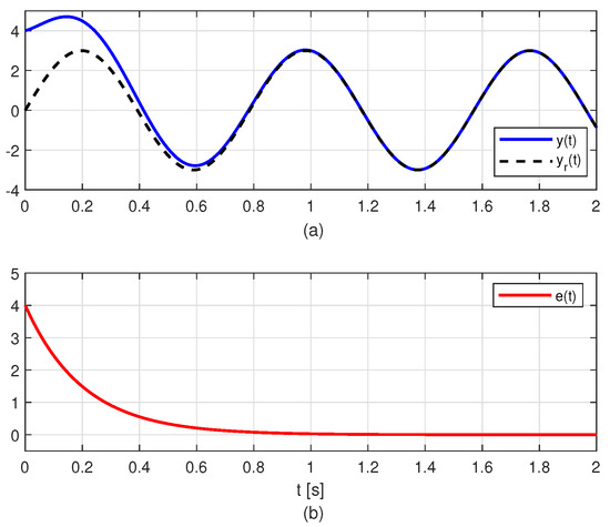
Figure 1. Regulator performance with $\mathsf{\Gamma }=[4.9348,8,-10]$: (a) Comparison of the output $y\left(t\right)$ and the reference $y_r\left(t\right)$, (b) Error between $y\left(t\right)$ and $y_r\left(t\right)$.

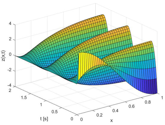
Figure 2. Spatial distribution of the solution surface corresponding to the rejection of constant disturbance.

To the case of trajectory tracking under the influence of harmonic disturbance, we set $M_d=1$, $A_r=3$, $A_d=3$, $\alpha =12$, $\beta =12$, $x_0=0.75$, $x_1=0.25$ and ${\nu }_0={\nu }_1=0.5$. Figure 3a shows the tracking of the reference signal $y_r\left(t\right)$ by the controlled output $y\left(t\right)$ for the initial condition $\phi \left(x\right)=4cos\left(\pi x\right)$. Figure 3b exhibits that $e\left(t\right)\to 0$ as $t\to \infty$. The corresponding solution surface is shown in Figure 4.

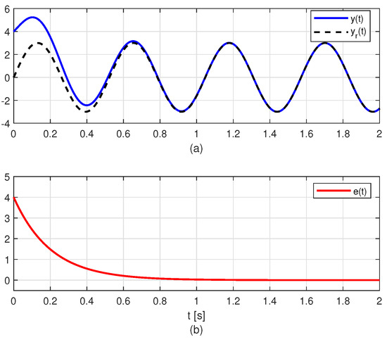
Figure 3. Regulator performance with $\mathsf{\Gamma }=[4.9348,12,-1,0]$: (a) Comparison of the output $y\left(t\right)$ and the reference signal $y_r\left(t\right)$, (b) Error between $y\left(t\right)$ and $y_r\left(t\right)$.

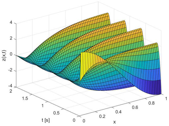
Figure 4. Spatial distribution of the solution surface related with the rejection of harmonic disturbance.

So, the regulator performs well under the presence of external disturbances for both cases, i.e., in the presence of either a constant disturbance or harmonic disturbance.

5. Conclusions

In our work, the SFRP approach is focused on the trajectory tracking control with the rejection of external disturbances to the C–D equation. The C–D system is modeled through a state operator given in the form of the SLDO plus an integral term involved in an abstract control system model from which the regulator equations are derived and solved. From the simulation results, it is concluded that our proposal performs well since when considering both constant and harmonic disturbances, the regulator is capable of tracking the reference trajectory, showing the rejection of external disturbances. As future work, we are focused on extend our proposal to multiple-input/multiple-output systems.

References

- Morris, K.A. Controller Design for Distributed Parameter Systems; Springer: Berlin/Heidelberg, Germany, 2020; pp. 59–67. [Google Scholar]
- Morris, K. Control of Systems Governed by Partial Differential Equations. In The Control Handbook, 2nd ed.; Levine, W.S., Ed.; CRC Press: Boca Raton, FL, USA, 2011; pp. 67-1–67-37. [Google Scholar]
- Isidori, A. Nonlinear Control Systems; Springer: London, UK, 1995. [Google Scholar]
- Pohjolainen, S.A. On the asymptotic regulation problem for distributed parameter systems. In Control of Distributed Parameter Systems; Pergamon: Oxford, UK, 1983; pp. 197–201. [Google Scholar]
- Pohjolainen, S.A. Robust multivariable PI–controller for infinite dimensional systems. IEEE Trans. Autom. Control 1982, 27, 17–30. [Google Scholar] [CrossRef]
- Schumacher, J.M. Dynamic feedback in finite– and infinite–dimensional linear systems. In Mathematisch Centrum Tracts; Centrum Voor Wiskunde en Informatica: Amsterdam, The Netherlands, 1981; Volume 143. [Google Scholar]
- Schumacher, J.M. Finite–dimensional regulators for a class of infinite–dimensional systems. Syst. Control. Lett. 1983, 3, 7–12. [Google Scholar] [CrossRef]
- Byrnes, C.I.; Laukó, I.G.; Gilliam, D.S.; Shubov, V.I. Output regulation for linear distributed parameter systems. IEEE Trans. Autom. Control 2000, 45, 2236–2252. [Google Scholar]
- Müller, P.H. “T. Kato, Perturbation theory for linear operators.(Die Grundlehren der mathematischen Wissenschaften in Einzeldarstellungen mit besonderer Berücksichtigung der Anwendungsgebiete, Band 132) XX+ 592 S. m. 3 Fig. Berlin/Heidelberg/New York Springer-Verlag. Preis geb. DM 79, 20”. Z. Angew. Math. Mech. 1967, 47, 554. [Google Scholar]
- Curtain, R.F.; Zwart, H. An Introduction to Infinite-Dimensional Linear Systems Theory; Springer: New York, NY, USA, 1995. [Google Scholar]
- Aulisa, E.; Gilliam, D. A Practical Guide to Geometric Regulation for Distributed Parameter Systems; CRC Press: Boca Raton, FL, USA, 2016. [Google Scholar]
- Natarajan, V.; Gilliam, D.S.; Weiss, G. The state feedback regulator problem for regular linear systems. IEEE Trans. Autom. Control 2014, 59, 2708–2723. [Google Scholar] [CrossRef]
- Xu, X.; Dubljevic, S. Output and error feedback regulator designs for linear infinite–dimensional systems. Automatica 2017, 83, 170–178. [Google Scholar] [CrossRef]
- Jurado, F.; Ramírez, A.A. State feedback regulation problem to the reaction-diffusion equation. Mathematics 2020, 8, 1983. [Google Scholar] [CrossRef]
- Ramírez, A.A.; Jurado, F. Tracking regulator design with disturbance rejection to the reaction–diffusion equation. In Proceedings of the 2019 16th International Conference on Electrical Engineering, Computing Science and Automatic Control (CCE), Mexico City, Mexico, 11–13 September 2019; pp. 11–13. [Google Scholar]
- Farlow, S.J. Partial Differential Equations for Scientists and Engineers; Dover Publications: New York, NY, USA, 1993. [Google Scholar]
- Hoteit, H. Modeling diffusion and gas–oil mass transfer in fractured reservoirs. J. Pet. Sci. Eng. 2013, 105, 1–17. [Google Scholar] [CrossRef]
- Deleuze, Y.; Chiang, C.-Y.; Thiriet, M.; Sheu, T.W.H. Numerical study of plume patterns in a chemotaxis–diffusion–convection coupling system. Comput. Fluids 2016, 126, 58–70. [Google Scholar] [CrossRef]
- Guenther, R.B.; Lee, J.W. Sturm–Liouville Problems Theory and Numerical Implementation; CRC Press: Boca Raton, FL, USA, 2019. [Google Scholar]
- Spiegel, M.R. Fourier Analysis with Applications to Boundary Value Problems; McGraw–Hill: New York, NY, USA, 1974. [Google Scholar]
- Kreyszig, E. Advanced Engineering Mathematics; John Wiley & Sons: Hoboken, NJ, USA, 2006. [Google Scholar]
- Mathews, J. Walker, R.L. Mathematical Methods of Physics; The Benjamin/Cummings Publishing Co.: Menlo Park, CA, USA, 1970. [Google Scholar]
- Holland, S.S., Jr. Applied Analysis by the Hilbert Space Method, An Introduction with Applications to the Wave, Heat, and Schrödinger Equations; Dover Publications: Mineola, NY, USA, 1990. [Google Scholar]
- Arfken, G.B.; Weber, H.J.; Harris, F.E. Mathematical Methods for Physicists A Comprehensive Guide; Academic Press: Waltham, MA, USA, 2013. [Google Scholar]
- Kaplan, K. Advanced Calculus; Pearson Education: Boston, MA, USA, 2003. [Google Scholar]
- Wyld, H.W. Mathematical Methods for Physics; CRC Press: Boca Raton, FL, USA, 2021. [Google Scholar]
- Pazy, A. Semigroups of Linear Operators and Applications to Partial Differential Equations; Springer: New York, NY, USA, 1983. [Google Scholar]
- Curtain, R.; Zwart, H. Introduction to Infinite-Dimensional Systems Theory; Springer: New York, NY, USA, 2020. [Google Scholar]
Disclaimer/Publisher’s Note: The statements, opinions and data contained in all publications are solely those of the individual author(s) and contributor(s) and not of MDPI and/or the editor(s). MDPI and/or the editor(s) disclaim responsibility for any injury to people or property resulting from any ideas, methods, instructions or products referred to in the content. |
© 2023 by the authors. Licensee MDPI, Basel, Switzerland. This article is an open access article distributed under the terms and conditions of the Creative Commons Attribution (CC BY) license (https://creativecommons.org/licenses/by/4.0/).