A Hybrid CM-BEM Formulation for Solving Large-Scale 3D Eddy-Current Problems Based on ℋ-Matrices and Randomized Singular Value Decomposition for BEM Matrix Compression

Abstract

We present a novel $a,v$-q hybrid method for solving large-scale time-harmonic eddy-current problems. This method combines a hybrid unsymmetric formulation based on the cell method and the boundary element method with a hierarchical matrix-compression technique based on randomized singular value decomposition. The main advantage is that the memory requirements are strongly reduced compared to the corresponding hybrid method without matrix compression while retaining the same robust solution strategy consisting of a simple construction of the preconditioner. In addition, the matrix-compression accuracy and efficiency are enhanced compared to traditional compression methods, such as adaptive cross approximation. The numerical results show that the proposed hybrid approach can also be effectively used to analyze large-scale eddy-current problems of engineering interest.

1. Introduction

Hybrid methods combining, e.g., the finite element method (FEM) and the boundary element method (BEM), can be very effective when solving electromagnetic problems since an air–region mesh is not needed and post-processing is much easier than pure FEM. They allow for an analytical computation of the magnetic field generated by sources, such as coils, which can be useful to reduce the model complexity. Moreover, hybrid approaches avoid the so-called truncation error, which is introduced in standard FEM by the use of an air domain of finite extent on which boundary conditions are applied. For the discretization of the magnetostatic problem in the unbounded exterior region, the BEM is used, whereas for the discretization of the field problem in the interior region, the FEM is typically used.

The cell method (CM), introduced by Tonti in [1], was proposed in [2] as an alternative to the FEM when devising hybrid formulations. The CM is a numerical method for solving boundary value problems (BVPs), which offers the following advantages: (1) equations are formulated directly in algebraic form suitable for numerical computations, (2) the continuity of tangent and normal field components between finite elements is naturally enforced by using integral variables (termed degrees of freedom, DOFs); (3) by using piecewise constant bases, as proposed in [3] for tetrahedral meshes and in [4] for general polyhedral meshes, the assembly of linear system matrices is completely Jacobian-free with great benefits in terms of the computation time and ease of implementation.

These peculiarities make the CM suitable for hybrid methods, where the continuity of field components at the interface between interior and exterior regions is enforced to couple differential and integral equation methods. Starting from these bases, a CM–BEM hybrid method for three-dimensional (3D) magnetostatic problems was proposed in [5]. As a main feature, a final symmetric linear system, amenable to the fast minimal residual method (MINRES) iterative solution, was obtained. This hybrid method was extended in [6] to the analysis of 3D time–harmonic electrothermal problems, leading to a final symmetric (complex valued) linear system, which could be solved by a fast transpose free quasi-minimal residual (TFQMR) solver. Both hybrid methods were formulated in terms of a variables (i.e., line integrals of the magnetic vector potential) in the interior region, and in terms of $\phi$ variables (i.e., magnetic scalar potentials) in the unbounded exterior region, yielding the so-called a-$\phi$ formulation.

Its main advantage is to minimize the number of DOFs used to represent the eddy-current problem, which is particularly convenient when using the BEM leading to dense matrices with huge memory occupation. On the other hand, due to the adoption of a scalar potential as a working variable, numerical analyses were limited to models geometries with simply-connected domains (e.g., without holes or handles). This limitation was removed in [7], where the a-$\phi$ formulation was extended to the most general case of multiply-connected domains.

More recently, a unified framework for devising hybrid formulations was proposed in [8]. Based on the concept of an augmented dual grid [9], i.e., a novel geometric setting for the CM, topological operators were introduced to consistently couple CM and BEM. This led to hybrid formulations with a final symmetric linear system amenable to fast TFQMR iterative solution. As a main outcome, direct and indirect hybrid formulations with comparable numerical performance and accuracy were obtained.

The main limitation to the applicability of hybrid methods to large-scale problems is represented by the high computation time and memory requirements implied in the assembly and storage of dense BEM matrices. The efficient treatment of matrices arising, e.g., from the finite element discretization of integral operators requires special compression techniques [10]. Among different approaches for matrix compression, the adaptive cross approximation (ACA) is know to be, by far, the most simple approach, and it is well-behaved in the low-frequency limit since $O(nlogn)$ computational complexity is attained [11].

By using the so-called $\mathcal{H}$-matrix format, dense BEM matrices are stored in a hierarchical tree of leaves (i.e., submatrices), where admissible leaves are approximated as low-rank matrices by using ACA, and inadmissible leaves are stored as they are without compression. In this way, off-diagonal blocks of a BEM matrix can be dramatically compressed via a low-rank approximation, and solution methods that scale up to millions of elements can be obtained.

Most of the papers in the literature concerning the solution of large-scale problems with dense matrix approximation deal with pure integral equation methods, such as the volume integral method (VIM) [12], the method of moment (MoM) [13], or the BEM [14], whereas only a few examples have been reported for hybrid methods. In [15], $\mathcal{H}$-matrices were used to provide a sparse representation of BEM dense matrices for a hybrid FEM–BEM approach for large-scale micromagnetic simulations.

In [16], a larger compression ratio was obtained by using hierarchical matrices of ${\mathcal{H}}^2$ type, i.e., an improved variant of $\mathcal{H}$-matrices exploiting an algebraic recompression technique. In such a way, test cases with more than one million DOFs were treated with negligible loss of accuracy compared to the uncompressed hybrid approach, and almost linear scaling in terms of allocated memory was attained. In [17], a direct FEM–BEM was combined with a $\mathcal{H}$-matrix-compression technique for the solution of magnetostatic problems. The final system of non-linear equations was solved by using a preconditioned generalized minimal residual (GMRES) Krylov subspace method.

To the authors’ knowledge, no hybrid approach to solve large-scale eddy current problems has been presented to date. This is likely due to the difficulty in finding a good preconditioner and an efficient iterative solver relying on $\mathcal{H}$-matrix algebra and also in finding a good compression technique for the BEM double-layer matrix. In particular, the a-$\phi$ direct and indirect formulations proposed in [8] are unsuited for matrix compression since they are based on matrix inversion to construct the discrete Steklov–Poincaré operator.

The main outcomes of this work are: (i) a novel hybrid formulation suitable for matrix compression that leads to a final linear system amenable to a fast TFQMR iterative solution and (ii) a novel $\mathcal{H}$-matrix-compression algorithm based on randomized singular value decomposition (R-SVD), which is more robust and faster than traditional ACA. The novel $a,v$-q hybrid formulation relies on the use of v variables (i.e., time-integrals of electric scalar potentials at mesh nodes in the conductive parts of the model) and q variables (i.e., fictitious magnetic charges on mesh triangles at the interface between interior and exterior regions).

The paper is structured as follows. The eddy current formulation, subdivided into interior and exterior field problems, is presented in a continuous setting in Section 2. The discretization of interior and exterior problems by using CM and BEM, respectively, is presented in Section 3, where the final unsymmetric linear system is derived. Section 4 presents a novel compression algorithm based on the use of R-SVD. The hybrid method is finally validated in Section 5, where both accuracy and compression performances of ACA and R-SVD algorithms are compared.

2. Eddy Current Problem

The computational domain of the hybrid formulation is unbounded, which is different from typical FEM formulations, and is subdivided into two different regions. The interior region contains conductive and/or magnetic materials, and is defined as the union of n open bounded and possibly multiply-connected subdomains ${\mathsf{\Omega }}_k\subset {\mathbb{R}}^3$, $k=1,\cdots ,n$—that is, $\mathsf{\Omega }={\bigcup }_{k=1}^n{\mathsf{\Omega }}_k$. In this way, $\mathsf{\Omega }$ can be made of handles and/or holes. The interior region can be partitioned into a conductive region ${\mathsf{\Omega }}_C$, with non-trivial electric conductivity, and an insulating region ${\mathsf{\Omega }}_I=\mathsf{\Omega }\backslash {\mathsf{\Omega }}_C$. The complement of the interior region is the exterior region ${\mathsf{\Omega }}_e={\mathbb{R}}^3\backslash \overline{\mathsf{\Omega }}$, where the bar notation indicates the set closure. ${\mathsf{\Omega }}_e$ is assumed to be insulating (i.e., made of air only), unbounded, and possibly multiply-connected. This means that there exists a loop in ${\mathsf{\Omega }}_e$, which cannot be shrunk to a point while remaining in ${\mathsf{\Omega }}_e$ [18]. The interface between $\mathsf{\Omega }$ and ${\mathsf{\Omega }}_e$ coincides with the boundary of $\mathsf{\Omega }$, i.e., $\Gamma =\partial \mathsf{\Omega }$.

2.1. Interior Field Problem

The magnetic diffusion equation in $\mathsf{\Omega }$ is formulated in terms of the magnetic vector potential $\mathbf{A}$ and the time-integral of the electric scalar potential V. The eddy current model is governed by Maxwell’s equations at low frequency, where the displacement current is neglected. By assuming linear media, i.e., piecewise locally constant material parameters (the electric conductivity $\sigma$ and the magnetic reluctivity $\nu$), and AC current-driven sources at constant angular frequency $\omega >0$, these can be expressed in the frequency domain as:

$$\begin{array}{cc}\hfill \nabla \times \mathbf{E}+ı\omega \mathbf{B}& \hfill =\mathbf{0},\hfill \end{array}$$

(1)

$$\begin{array}{cc}\hfill \nabla \times \mathbf{H}& \hfill =\mathbf{J},\hfill \end{array}$$

(2)

$$\begin{array}{cc}\hfill \hspace{1em}\hspace{1em}\hspace{1em}\hspace{1em} \mathbf{J}& \hfill =\sigma \mathbf{E},\hfill \end{array}$$

(3)

$$\begin{array}{cc}\hfill \hspace{1em}\hspace{1em}\hspace{1em} \mathbf{H}& \hfill =\nu \mathbf{B},\hfill \end{array}$$

(4)

where ı is the imaginary unit. In Maxwell’s equations, $\mathbf{E}$ is the electric field, $\mathbf{B}$ is the magnetic flux density, $\mathbf{H}$ is the magnetic field, and $\mathbf{J}$ is the induced current density. By noting from (1) that $\mathbf{B}$ is div-free, the magnetic vector potential can be introduced as:

$$\mathbf{B}=\nabla \times \mathbf{A}.$$

(5)

By inserting (5) in (1), the field $\mathbf{E}+ı\omega \mathbf{B}$ results as curl-free, and thus an electric scalar potential can be introduced as:

$$\mathbf{E}=-ı\omega \left(\mathbf{A}+\nabla V\right),$$

(6)

which is equivalent to (1). By inserting (6) in (3) and by substituting (5) in (4), (2) can be rephrased as the so-called magnetic diffusion equation:

$$\nabla \times \nu \nabla \times \mathbf{A}+ı\omega \sigma \left(\mathbf{A}+\nabla V\right)=\mathbf{0},$$

(7)

describing the magnetic field diffusion inside $\mathsf{\Omega }$. By imposing the div-free condition $\nabla ·\mathbf{J}=0$ resulting from (2), the electric scalar potential is constrained in ${\mathsf{\Omega }}_C$ as:

$$-ı\omega \nabla ·\sigma \left(\mathbf{A}+\nabla V\right)=0.$$

(8)

In this way, the electric vector potential is undefined in ${\mathsf{\Omega }}_I$, where $\sigma =0$.

2.2. Exterior Field Problem

The magnetic field in ${\mathsf{\Omega }}_e$ is governed by the equation of magnetostatics:

$$\begin{array}{cc}\hfill \nabla \times \mathbf{H}& \hfill ={\mathbf{J}}_{\mathbf{0}},\hfill \end{array}$$

(9)

$$\begin{array}{cc}\hfill \nabla ·\mathbf{B}& \hfill =\mathbf{0},\hfill \end{array}$$

(10)

$$\begin{array}{cc}\hfill \hspace{1em}\hspace{1em}\hspace{1em} \mathbf{B}& \hfill ={\mu }_0\mathbf{H}.\hfill \end{array}$$

(11)

The source current density ${\mathbf{J}}_0$ is assumed to be known at any point of the source region ${\mathsf{\Omega }}_0\subseteq {\mathsf{\Omega }}_e$ and represents magnetic field sources at low frequency, such as current-driven coils. In particular, the skin-effect in ${\mathsf{\Omega }}_0$ is neglected, which is reasonable for stranded coils.

As proposed in [7], the magnetic field in ${\mathsf{\Omega }}_e$ can be obtained from the reduced magnetic scalar potential $\phi$ by solving the Exterior Neumann problem (ENP), which is defined as follows. The source magnetic field can be analytically computed by Biot–Savart’s law as:

$${\mathbf{H}}_0\left(x\right)={\int }_{{\mathsf{\Omega }}_0}\frac{{\mathbf{J}}_0\left(y\right)\times (x-y)}{{\parallel x-y\parallel }^3}dy,\mathrm{for}\mathrm{any}x\in {\mathbb{R}}^3\backslash {\overline{\mathsf{\Omega }}}_0.$$

(12)

By using (9) and noting that $\nabla \times {\mathbf{H}}_0={\mathbf{J}}_0$, the reduced field ${\mathbf{H}}_r=\mathbf{H}-{\mathbf{H}}_0$ is found to be curl-free. From homological algebra, it is known that any curl-free field is a representative of the first de Rham cohomology group $H_{dR}^1\left({\mathsf{\Omega }}_e\right)$[19]. This group is finitely generated by a vector basis $\left[{\mathbf{h}}_k\right]$, $k=1,\cdots ,{\beta }_1$, where ${\mathbf{h}}_k$ are representatives of the cohomology group, i.e., the so-called cohomology generators, and the square bracket notation denotes cosets. Due to de Rham’s theorem, i.e., $H_{dR}^1\left({\mathsf{\Omega }}_e\right)\cong H^1\left({\mathsf{\Omega }}_e\right)$, and Alexander duality, i.e., $H^1\left({\mathsf{\Omega }}_e\right)\cong H_1\left(\mathsf{\Omega }\right)$, the dimension of the de Rham cohomology group is equal to that of the first homology group $H_1\left(\mathsf{\Omega }\right)$, which is defined as the first Betti number${\beta }_1$ [20].

By noting that $\left[{\mathbf{H}}_r\right]\in H_{dR}^1\left({\mathsf{\Omega }}_e\right)$, the magnetic field in ${\mathsf{\Omega }}_e$ can be expanded as:

$$\mathbf{H}={\mathbf{H}}_0-\nabla \phi +\sum _{k=1}^{{\beta }_1}{I}_k{\mathbf{h}}_k,$$

(13)

where $I_k$, $k=1,\cdots ,{\beta }_1$, are complex coefficients. It is proven in [7] that these have true physical meaning, i.e., $I_k$ are eddy currents through an independent cut set ${\Sigma }_k$ of $\mathsf{\Omega }$. As described in [21], any cut surface ${\Sigma }_k$ is in one-to-one correspondence to a non-bounding loop in $\mathsf{\Omega }$, ${\gamma }_k$, i.e., a generator of $H_1\left(\mathsf{\Omega }\right)$. Cohomology generators in (13) can be built, for instance, from Biot–Savart’s law as [20]:

$${\mathbf{h}}_k\left(x\right)={\int }_{{\gamma }_k}\frac{{\mathbf{t}}_k\left(y\right)\times (x-y)}{{\parallel x-y\parallel }^3}d{\gamma }_y,\mathrm{for}\mathrm{any}x\in {\mathsf{\Omega }}_e,$$

(14)

where ${\mathbf{t}}_k$ is the unit vector tangent to ${\gamma }_k$.

Additional degrees of freedom required for representing the magnetic field in (13) are enforced by using the following topological constraints [7]:

$${\int }_{{\mathsf{\Omega }}_e}{\mathbf{h}}_k·\left(\mathbf{B}-\nabla \times \mathbf{A}\right)d\mathsf{\Omega }=0,k=1,\cdots ,{\beta }_1.$$

(15)

By inserting (13) in (11), and by noting that ${\mathbf{H}}_0$ and ${\mathbf{h}}_k$ are div-free fields, from (10), the following Laplace’s equation is obtained:

$$\nabla ·\left(-{\mu }_0\nabla \phi \right)=0.$$

(16)

The ENP is formed by taking (16), the radiation condition $\phi \left(x\right)=\mathcal{O}\left(\right|x{|}^{-1})$ for $\left|x\right|\to \infty$ and the Neumann boundary condition on $\Gamma$:

$${\partial }_n\phi =-B_{r,n},$$

(17)

where ${\partial }_n$ indicates the normal derivative along the unit normal vector $\mathbf{n}$ (pointing outward from $\mathsf{\Omega }$), and $B_{r,n}={\mu }_0{\mathbf{H}}_r·\mathbf{n}$ is the normal component of the magnetic flux density. Equation (16) can be solved, for instance, by using an indirect approach, which introduces a fictitious unknown. According to the method of layer potentials, the ENP is transformed into an equivalent Fredholm integral equation [22]:

$${\mu }_{0}c\left(x\right)q\left(x\right)+{\mathcal{T}}^{*}\left[q\right]\left(x\right)=B_{r,n}\left(x\right),\mathrm{for}\mathrm{a}.\mathrm{a}.x\in \Gamma ,$$

(18)

to be solved in terms of an equivalent charge distribution q on $\Gamma$. The coefficient $c=\alpha /\left(4\pi \right)$ is a geometric factor, where $\alpha$ is the solid angle approaching $\Gamma$ from ${\mathsf{\Omega }}_e$. The second term in (18) is the adjoint double–layer integral operator [22]:

$${\mathcal{T}}^{*}\left[q\right]\left(x\right)=-{\mu }_0{\int }_{\Gamma }q\left(y\right)\frac{\partial \mathsf{\Phi }(x,y)}{\partial n_x}d{\sigma }_y,$$

(19)

where $\mathsf{\Phi }(x,y)={\left(4\pi |x-y|\right)}^{-1}$ is the fundamental solution for the 3D Laplacian, and $\partial /\partial n_x$ is the normal derivative evaluated with respect to the x variable. Finally, once (18) has been solved, $\phi$ can be reconstructed in the whole region ${\mathsf{\Omega }}_e$ from q by using the single-layer integral operator with moment q:

$$\phi \left(x\right)=K\left[q\right]\left(x\right)={\int }_{\Gamma }\mathsf{\Phi }(x,y)q\left(y\right)d{\sigma }_y.$$

(20)

2.3. Transmission Conditions

The interior and exterior field problems are coupled by enforcing transmission conditions through $\Gamma$. After defining the trace operators for Dirichlet (D) and Neumann (N) conditions for any smooth field $\mathbf{U}$ defined on $\Gamma$:

$$\begin{array}{cc}\hfill {\gamma }_D\mathbf{U}& \hfill =\left(\mathbf{n}\times \mathbf{U}\right)\times \mathbf{n},\hfill \end{array}$$

(21)

$$\begin{array}{cc}\hfill {\gamma }_N\mathbf{U}& \hfill =\left(\nabla \times \mathbf{U}\right)\times \mathbf{n},\hfill \end{array}$$

(22)

the continuity of the normal component of $\mathbf{B}$ and of the tangent component of $\mathbf{H}$ can be expressed as:

$$\begin{array}{cc}\hfill {\gamma }_D^{-}\mathbf{A}& \hfill ={\gamma }_D^{+}\mathbf{A},\hfill \end{array}$$

(23)

$$\begin{array}{cc}\hfill \nu {\gamma }_N^{-}\mathbf{A}& \hfill ={\nu }_0{\gamma }_N^{+}\mathbf{A},\hfill \end{array}$$

(24)

where ${\nu }_0$ is the air reluctivity, and ± indicate the positive and negative sides of $\Gamma$ (e.g., with + the interface is approached from outside along the direction orthogonal to the interface).

3. Hybrid Formulation

The hybrid formulation is constructed by using the discretization framework described in [8] and briefly summarized here. The magnetic diffusion Equation (7) describing eddy currents in the interior region is discretized by using the CM, whereas the Fredholm integral Equation (18) is approximated by using the collocation BEM. Finally, discretized interior and exterior problems are coupled by means of transmission conditions, i.e., the conservation of both magnetic fluxes and magnetomotive forces at the interface.

3.1. Discrete Interior Problem

The interior region is meshed into tetrahedral cells that yield the so-called primal grid ${\mathcal{G}}_{\mathsf{\Omega }}$. The corresponding dual grid ${\tilde{\mathcal{G}}}_{\mathsf{\Omega }}$ is obtained from the barycentric dual complex related to ${\mathcal{G}}_{\mathsf{\Omega }}$. Primal and dual grids for subdomains ${\mathsf{\Omega }}_C$ and ${\mathsf{\Omega }}_I$ are obtained in the same way. Therefore the primal grid ${\mathcal{G}}_{{\mathsf{\Omega }}_C}$ is a subset of ${\mathcal{G}}_{\mathsf{\Omega }}$, and the corresponding dual grid ${\tilde{\mathcal{G}}}_{{\mathsf{\Omega }}_C}$ is a subset of ${\tilde{\mathcal{G}}}_{\mathsf{\Omega }}$. For coupling interior and exterior field problems at the discrete level, the interface primal grid ${\mathcal{G}}_{\Gamma }$ and the corresponding dual grid ${\tilde{\mathcal{G}}}_{\Gamma }$ are also introduced.

Any physical field is locally approximated by using linear combinations of piecewise constant bases defined in [3]. The coefficients of these combinations are related to geometric entities of either primal or dual grids (i.e., potential on nodes, line integrals, and fluxes through faces) and can be assembled into an array of DOFs—namely, discrete fields globally representing physical fields. Differential operators are approximated as incidence matrices, made up of $0, \pm 1$ coefficients. Constitutive relationships are approximated as positive-definite matrices due to the energy preserving property of piecewise constant bases. A linear system is finally obtained from topological and constitutive relationships in matrix form. From the linear system solution, the physical field can be locally reconstructed by using linear combinations of piecewise constant bases.

The time-harmonic eddy-current problem in $\mathsf{\Omega }$ is formulated in terms of line integrals of the magnetic vector potential, i.e., the array ${\mathbf{a}}_{\mathsf{\Omega }}={\left(a_e\right)}_{e\in {\mathcal{G}}_{\mathsf{\Omega }}}$ with $a_e={\int }_e\mathbf{A}·d\mathbf{l}$ integral along edge e. By integrating (6) along each primal edge, electromotive forces (EMFs) become:

$${\mathbf{e}}_{\mathsf{\Omega }}=-ı\omega \left({\mathbf{a}}_{\mathsf{\Omega }}+{\mathbf{G}}_{\mathsf{\Omega }}{\mathbf{v}}_{\mathsf{\Omega }}\right),$$

(25)

where ${\mathbf{v}}_{\mathsf{\Omega }}={\left(V\left(x_n\right)\right)}_{n\in {\mathcal{G}}_{\mathsf{\Omega }}}$ is the array of electric scalar potentials evaluated at primal nodes $x_n$, and ${\mathbf{G}}_{\mathsf{\Omega }}$ is the edge-to-node incidence matrix of ${\mathcal{G}}_{\mathsf{\Omega }}$ or primal gradient matrix. By integrating (5) over each primal face and by using Stokes’ theorem, magnetic fluxes become:

$${\mathbf{b}}_{\mathsf{\Omega }}={\mathbf{C}}_{\mathsf{\Omega }}{\mathbf{a}}_{\mathsf{\Omega }},$$

(26)

where ${\mathbf{C}}_{\mathsf{\Omega }}$ is the face-to-edge incidence matrix of ${\mathcal{G}}_{\mathsf{\Omega }}$ or primal curl matrix. Local constitutive equations are discretized by means of piecewise constant basis functions (namely, edge ${\mathbf{w}}^e$ and face ${\mathbf{w}}^f$ elements), which yield the conductance matrix ${\mathbf{M}}_{\sigma ,\mathsf{\Omega }}={\left(m_{\sigma ,e{e}^{\prime }}\right)}_{e,e^{\prime }\in {\mathcal{G}}_{\mathsf{\Omega }}}$ and the reluctance matrix ${\mathbf{M}}_{\nu ,\mathsf{\Omega }}={\left(m_{\nu ,f{f}^{\prime }}\right)}_{f,f^{\prime }\in {\mathcal{G}}_{\mathsf{\Omega }}}$, where $m_{\sigma ,e{e}^{\prime }}={\int }_{\mathsf{\Omega }}\sigma {\mathbf{w}}_e^e\left(x\right)·{\mathbf{w}}_{e^{\prime }}^e\left(x\right)dx$ and $m_{\nu ,f{f}^{\prime }}={\int }_{\mathsf{\Omega }}\nu {\mathbf{w}}_f^f\left(x\right)·{\mathbf{w}}_{f^{\prime }}^f\left(x\right)dx$. The local electric (3) and magnetic (4) constitutive relationships, after discretization on ${\mathcal{G}}_{\mathsf{\Omega }}$, become:

$$\begin{array}{cc}\hfill {\tilde{\mathbf{j}}}_{\mathsf{\Omega }}& \hfill ={\mathbf{M}}_{\sigma ,\mathsf{\Omega }}{\mathbf{e}}_{\mathsf{\Omega }},\hfill \end{array}$$

(27)

$$\begin{array}{cc}\hfill {\tilde{\mathbf{h}}}_{\mathsf{\Omega }}& \hfill ={\mathbf{M}}_{\nu ,\mathsf{\Omega }}{\mathbf{b}}_{\mathsf{\Omega }},\hfill \end{array}$$

(28)

where ${\tilde{\mathbf{j}}}_{\mathsf{\Omega }}={\left(j_{\tilde{f}}\right)}_{\tilde{f}\in {\tilde{\mathcal{G}}}_{\mathsf{\Omega }}}$ is the array of currents $j_{\tilde{f}}={\int }_{\tilde{f}}\mathbf{J}·d\mathbf{s}$ through faces $\tilde{f}$ of ${\tilde{\mathcal{G}}}_{\mathsf{\Omega }}$ and ${\tilde{\mathbf{h}}}_{\mathsf{\Omega }}={\left(h_{\tilde{e}}\right)}_{\tilde{e}\in {\tilde{\mathcal{G}}}_{\mathsf{\Omega }}}$ is the array of magnetomotive forces (MMFs) $h_{\tilde{e}}={\int }_{\tilde{e}}\mathbf{H}·d\mathbf{l}$ along any edge $\tilde{e}$ of ${\tilde{\mathcal{G}}}_{\mathsf{\Omega }}$. Coefficients of ${\mathbf{M}}_{\sigma ,\mathsf{\Omega }}$ are non-zero only in correspondence of primal edges of ${\mathcal{G}}_{{\mathsf{\Omega }}_C}$. By integrating (2) over each dual face and by using Stokes’ theorem, (2) can be discretized over ${\tilde{\mathcal{G}}}_{\mathsf{\Omega }}$ as:

$${\tilde{\mathbf{C}}}_{\mathsf{\Omega }}{\tilde{\mathbf{h}}}_{\mathsf{\Omega }}+{\tilde{\mathbf{C}}}_{\mathsf{\Omega }\Gamma }{\tilde{\mathbf{h}}}_{\Gamma }={\tilde{\mathbf{j}}}_{\mathsf{\Omega }},$$

(29)

where ${\tilde{\mathbf{C}}}_{\mathsf{\Omega }}={\mathbf{C}}_{\mathsf{\Omega }}^{\mathrm{T}}$ is the face-to-edge incidence matrix of ${\tilde{\mathcal{G}}}_{\mathsf{\Omega }}$ or dual curl matrix, and ${\tilde{\mathbf{C}}}_{\mathsf{\Omega }\Gamma }$ is the surface curl matrix, i.e., the transpose of the selection matrix (made up of $0,1$ coefficients), which extracts edges of ${\mathcal{G}}_{\Gamma }$ from those of ${\mathcal{G}}_{\mathsf{\Omega }}$. Coefficients of ${\tilde{\mathbf{h}}}_{\Gamma }$ are MMFs computed along the edges of ${\tilde{\mathcal{G}}}_{\Gamma }$ and are useful for coupling the interior (CM) and the exterior (BEM) field problems. Note that currents in (29) are due only to electromagnetic induction, i.e., they are eddy currents, because magnetic field sources are assumed to be in the exterior region.

The discrete diffusion equation is obtained by letting (27) and (28) in (29) and by expressing EMFs and magnetic fluxes in terms of potentials by (25) and (26). One obtains:

$$\left({\mathbf{C}}_{\mathsf{\Omega }}^{\mathrm{T}}{\mathbf{M}}_{\nu ,\mathsf{\Omega }}{\mathbf{C}}_{\mathsf{\Omega }}+ı\omega {\mathbf{M}}_{\sigma ,\mathsf{\Omega }}\right){\mathbf{a}}_{\mathsf{\Omega }}+ı\omega {\mathbf{M}}_{\sigma ,\mathsf{\Omega }}{\mathbf{G}}_{\mathsf{\Omega }}{\mathbf{v}}_{\mathsf{\Omega }}+{\tilde{\mathbf{C}}}_{\mathsf{\Omega }\Gamma }{\tilde{\mathbf{h}}}_{\Gamma }=\mathbf{0}.$$

(30)

By integrating (8) on each cell of ${\tilde{\mathcal{G}}}_{\mathsf{\Omega }}$ and by using Stokes’ theorem, the electric conservation equation at the discrete level becomes:

$$-ı\omega {\tilde{\mathbf{D}}}_{\mathsf{\Omega }}{\mathbf{M}}_{\sigma ,\mathsf{\Omega }}\left({\mathbf{a}}_{\mathsf{\Omega }}+{\mathbf{G}}_{\mathsf{\Omega }}{\mathbf{v}}_{\mathsf{\Omega }}\right)=\mathbf{0},$$

(31)

where ${\tilde{\mathbf{D}}}_{\mathsf{\Omega }}=-{\mathbf{G}}_{\mathsf{\Omega }}^{\mathrm{T}}$ is the cell-to-face incidence matrix of ${\tilde{\mathcal{G}}}_{\mathsf{\Omega }}$. Equation (31) provides additional constraints required for introducing the electric scalar potential in $\mathsf{\Omega }$.

3.2. Discrete Exterior Problem

The Fredholm Equation (18) is approximated by using collocation BEM. The reduced magnetic flux through any primal face f of the primal interface grid ${\mathcal{G}}_{\Gamma }$, i.e., the boundary of ${\mathcal{G}}_{\mathsf{\Omega }}$ is obtained as:

$$b_{r,f}={\int }_f{B}_{r,n}\left(x\right)d{\sigma }_x={\int }_f{\mu }_{0}c\left(x\right)q\left(x\right)+{\mathcal{T}}^{*}\left[q\right]\left(x\right)d{\sigma }_x,$$

(32)

which can be approximated by assuming a linear variation of $B_{r,n}$ on f, as:

$$b_{r,f}\approx \left|f\right|B_{r,n}\left({\tilde{x}}_f\right)=\frac{{\mu }_0\left|f\right|}{2}{q}_f-{\mu }_0\mathbf{f}·{\sum }_{f^{\prime }\in {\mathcal{G}}_{\Gamma }}^{}\left({\int }_{f^{\prime }}\nabla {}_x\mathsf{\Phi }({\tilde{x}}_f,y)d{\sigma }_y\right)q_{f^{\prime }},$$

(33)

where $B_{r,n}$ is evaluated at the face center ${\tilde{x}}_f$, $\left|f\right|$ is the face area, $\mathbf{f}$ is the face vector of f, and $q_{f^{\prime }}$ is the magnetic charge on the source face $f^{\prime }$. The sum in (33) is performed over the faces of ${\mathcal{G}}_{\Gamma }$, and the operator $\nabla {}_x$ indicates the gradient evaluated with respect to the x variable only. Equation (33) can be assembled over the whole interface grid as:

$${\mathbf{b}}_{r,\Gamma }={\mathbf{V}}_{\Gamma }{\mathbf{q}}_{\Gamma },$$

(34)

where ${\mathbf{b}}_{r,\Gamma }={\left(b_{r,f}\right)}_{f\in {\mathcal{G}}_{\Gamma }}$ and ${\mathbf{q}}_{\Gamma }={\left(q_f\right)}_{f\in {\mathcal{G}}_{\Gamma }}$ are the arrays of reduced magnetic fluxes and charges on interface primal faces, respectively. The double-layer matrix ${\mathbf{V}}_{\Gamma }={\left(v_{f,f^{\prime }}\right)}_{f,f^{\prime }\in {\mathcal{G}}_{\Gamma }}$ is defined as:

$$v_{f{f}^{\prime }}=\frac{{\mu }_0\left|f\right|}{2}{\delta }_{f{f}^{\prime }}-{\mu }_0\mathbf{f}·{\int }_{f^{\prime }}\nabla {}_x\mathsf{\Phi }({\tilde{x}}_f,y)d{\sigma }_y,$$

(35)

where ${\delta }_{f{f}^{\prime }}$ is the Kronecker delta, i.e., if source and induced face coincide ($f=f^{\prime }$), then ${\delta }_{f{f}^{\prime }}=1$, and zero otherwise. On the other hand, by evaluating the scalar potential at dual nodes ${\tilde{x}}_f$ according to the collocation method, (20) can be approximated as:

$$\phi \left({\tilde{x}}_f\right)={\int }_{\Gamma }\mathsf{\Phi }({\tilde{x}}_f,y)q\left(y\right)d{\sigma }_y.$$

(36)

Equation (36) assembled over the entire grid ${\mathcal{G}}_{\Gamma }$ becomes:

$${\tilde{\mathbf{\phi }}}_{\Gamma }={\mathbf{K}}_{\Gamma }{\mathbf{q}}_{\Gamma },$$

(37)

where ${\tilde{\mathbf{\phi }}}_{\Gamma }={\left(\phi \left({\tilde{x}}_f\right)\right)}_{f\in {\mathcal{G}}_{\Gamma }}$ is the array of reduced magnetic potentials evaluated at dual nodes ${\tilde{x}}_f)$ of ${\tilde{\mathcal{G}}}_{\Gamma }$, i.e., the centers of primal faces of ${\mathcal{G}}_{\Gamma }$, and the single-layer matrix ${\mathbf{K}}_{\Gamma }={\left(k_{f,f^{\prime }}\right)}_{f,f^{\prime }\in {\mathcal{G}}_{\Gamma }}$ has the coefficients:

$$k_{f{f}^{\prime }}={\int }_{f^{\prime }}\mathsf{\Phi }({\tilde{x}}_f,y)d{\sigma }_y.$$

(38)

3.3. Coupled Problem

For coupling the discrete interior and exterior field problems, transmission conditions at the interface grid are used. By integrating (23) through faces of ${\mathcal{G}}_{\Gamma }$ and (24) along the edges of ${\tilde{\mathcal{G}}}_{\Gamma }$, respectively, and by using the magnetic field decomposition (13), the arrays of magnetic fluxes and MMFs of ${\mathcal{G}}_{\Gamma }$ are obtained:

$$\begin{array}{cc}\hfill {\mathbf{b}}_{\Gamma }& \hfill ={\mathbf{b}}_{0,\Gamma }+{\mathbf{b}}_{r,\Gamma }+\sum _{k=1}^{{\beta }_1}{I}_k{\mathbf{b}}_{k,\Gamma },\hfill \end{array}$$

(39)

$$\begin{array}{cc}\hfill {\tilde{\mathbf{h}}}_{\Gamma }& \hfill ={\tilde{\mathbf{h}}}_{0,\Gamma }+{\tilde{\mathbf{h}}}_{r,\Gamma }+\sum _{k=1}^{{\beta }_1}{I}_k{\tilde{\mathbf{h}}}_{k,\Gamma }.\hfill \end{array}$$

(40)

The arrays of the total magnetic fluxes ${\mathbf{b}}_{\Gamma }$, source magnetic fluxes ${\mathbf{b}}_{0,\Gamma }$, and topological magnetic fluxes ${\mathbf{b}}_{k,\Gamma }$ in (39) can be expressed all in same way by using Stokes’ theorem, e.g.,

$${\mathbf{b}}_{\Gamma }={\mathbf{C}}_{\Gamma }{\mathbf{a}}_{\Gamma },$$

(41)

where ${\mathbf{C}}_{\Gamma }$ is the face-to-edge incidence matrix related to ${\mathcal{G}}_{\Gamma }$. Terms related to virtual loops ${\mathbf{a}}_{k,\Gamma }$ and ${\tilde{\mathbf{h}}}_{k,\Gamma }$ are computed by taking the line integrals of the virtual magnetic vector potential ${\mathbf{a}}_k\left(x\right)={\int }_{{\gamma }_k}{\mathbf{t}}_k\left(y\right)/\parallel x-y\parallel dy$ and the virtual magnetic field (14) along the primal edges and dual edges at the interface, respectively. ${\mathbf{a}}_{0,\Gamma }$ and ${\tilde{\mathbf{h}}}_{0,\Gamma }$ are computed from the source current density by a numerical quadrature of Biot–Savart’s law. The reduced MMFs are expressed as a function of magnetic potentials on dual nodes as:

$${\tilde{\mathbf{h}}}_{r,\Gamma }={\tilde{\mathbf{G}}}_{\Gamma }{\tilde{\mathbf{\phi }}}_{\Gamma },$$

(42)

where ${\tilde{\mathbf{G}}}_{\Gamma }={\mathbf{C}}_{\Gamma }^{\mathrm{T}}$ is the dual edge-node incidence matrix of ${\tilde{\mathcal{G}}}_{\Gamma }$. Boundary DOFs can be extracted from bulk ones by using a selection matrix, as ${\mathbf{a}}_{\Gamma }={\tilde{\mathbf{C}}}_{\mathsf{\Omega }\Gamma }^{\mathrm{T}}{\mathbf{a}}_{\mathsf{\Omega }}$. By letting (34) in (39) and (37) in (40), transmission conditions become:

$$\begin{array}{cc}\hfill {\mathbf{C}}_{\Gamma }{\tilde{\mathbf{C}}}_{\mathsf{\Omega }\Gamma }^{\mathrm{T}}{\mathbf{a}}_{\mathsf{\Omega }}& \hfill ={\mathbf{C}}_{\Gamma }{\mathbf{a}}_{0,\Gamma }+{\mathbf{V}}_{\Gamma }{\mathbf{q}}_{\Gamma }+{\mathbf{C}}_{\Gamma }\sum _{k=1}^{{\beta }_1}{I}_k{\mathbf{a}}_{k,\Gamma },\hfill \end{array}$$

(43)

$$\begin{array}{cc}\hfill {\tilde{\mathbf{h}}}_{\Gamma }& \hfill ={\tilde{\mathbf{h}}}_{0,\Gamma }+{\tilde{\mathbf{G}}}_{\Gamma }{\mathbf{K}}_{\Gamma }{\mathbf{q}}_{\Gamma }+\sum _{k=1}^{{\beta }_1}{I}_k{\tilde{\mathbf{h}}}_{k,\Gamma }.\hfill \end{array}$$

(44)

By defining topological matrices

$$\begin{array}{cc}\hfill {\mathbf{A}}_{\Gamma }& \hfill =\left[{\mathbf{a}}_{1,\Gamma },\cdots ,{\mathbf{a}}_{{\beta }_1,\Gamma }\right],\hfill \end{array}$$

(45)

$$\begin{array}{cc}\hfill {\tilde{\mathbf{H}}}_{\Gamma }& \hfill =\left[{\tilde{\mathbf{h}}}_{1,\Gamma },\cdots ,{\tilde{\mathbf{h}}}_{{\beta }_1,\Gamma }\right],\hfill \end{array}$$

(46)

and the array of virtual currents ${\mathbf{I}}_{\gamma }={\left[I_1,\cdots ,I_{{\beta }_1}\right]}^{\mathrm{T}}$, transmission conditions can be rewritten more compactly as:

$$\begin{array}{cc}\hfill {\mathbf{C}}_{\Gamma }{\tilde{\mathbf{C}}}_{\mathsf{\Omega }\Gamma }^{\mathrm{T}}{\mathbf{a}}_{\mathsf{\Omega }}& \hfill ={\mathbf{C}}_{\Gamma }{\mathbf{a}}_{0,\Gamma }+{\mathbf{V}}_{\Gamma }{\mathbf{q}}_{\Gamma }+{\mathbf{C}}_{\Gamma }{\mathbf{A}}_{\Gamma }{\mathbf{I}}_{\gamma },\hfill \end{array}$$

(47)

$$\begin{array}{cc}\hfill {\tilde{\mathbf{h}}}_{\Gamma }& \hfill ={\tilde{\mathbf{h}}}_{0,\Gamma }+{\tilde{\mathbf{G}}}_{\Gamma }{\mathbf{K}}_{\Gamma }{\mathbf{q}}_{\Gamma }+{\tilde{\mathbf{H}}}_{\Gamma }{\mathbf{I}}_{\gamma }.\hfill \end{array}$$

(48)

Additional constraints required to account for topology are obtained from the discretization of (15) with edge elements. Topological relationships for ${\mathbf{I}}_{\gamma }$ are (for details, see [7]):

$${\tilde{\mathbf{h}}}_{k,\Gamma }^{\mathrm{T}}{\mathbf{a}}_{\Gamma }-{\mathbf{a}}_{k,\Gamma }^{\mathrm{T}}{\tilde{\mathbf{h}}}_{r,\Gamma }-\sum _{j=1}^{{\beta }_1}\left({\mathbf{a}}_{k,\Gamma }^{\mathrm{T}}{\tilde{\mathbf{h}}}_{j,\Gamma }\right)I_j={\tilde{\mathbf{h}}}_{0,\Gamma }^{\mathrm{T}}{\mathbf{a}}_{k,\Gamma }+a_{0,{\gamma }_k},k=1,\cdots ,{\beta }_1,$$

(49)

where the coefficients $a_{0,{\gamma }_k}$, $k=1,\cdots ,{\beta }_1\left(\mathsf{\Omega }\right)$ are the line integral (numerically computed) of the source magnetic vector potential along virtual loops ${\gamma }_k$. By using the definitions of topological matrices and by letting (37) and (42) in (49), topological constraints can be assembled into a unique matrix equation as:

$${\tilde{\mathbf{H}}}_{\Gamma }^{\mathrm{T}}{\tilde{\mathbf{C}}}_{\mathsf{\Omega }\Gamma }^{\mathrm{T}}{\mathbf{a}}_{\mathsf{\Omega }}-{\mathbf{A}}_{\Gamma }^{\mathrm{T}}{\tilde{\mathbf{G}}}_{\Gamma }{\mathbf{K}}_{\Gamma }{\mathbf{q}}_{\Gamma }-{\mathbf{A}}_{\Gamma }^{\mathrm{T}}{\tilde{\mathbf{H}}}_{\Gamma }{\mathbf{I}}_{\gamma }={\mathbf{A}}_{\Gamma }^{\mathrm{T}}{\tilde{\mathbf{h}}}_{0,\Gamma }+{\mathbf{a}}_{0,\gamma }.$$

(50)

By inserting (48) in (30) and by using (31), (47), and (50), the final (unsymmetric and complex valued) linear system for the hybrid formulation is obtained:

$$\left(\begin{array}{cccc}{\mathbf{K}}_{11}& {\mathbf{K}}_{12}& {\mathbf{K}}_{13}& {\mathbf{K}}_{14}\\ {\mathbf{K}}_{21}& {\mathbf{K}}_{22}& \mathbf{0}& \mathbf{0}\\ {\mathbf{K}}_{31}& \mathbf{0}& {\mathbf{K}}_{33}& {\mathbf{K}}_{34}\\ {\mathbf{K}}_{41}& \mathbf{0}& {\mathbf{K}}_{43}& {\mathbf{K}}_{44}\end{array}\right)\left(\begin{array}{c}{\mathbf{a}}_{\mathsf{\Omega }}\\ {\mathbf{v}}_{\mathsf{\Omega }}\\ {\mathbf{q}}_{\Gamma }\\ {\mathbf{I}}_{\gamma }\end{array}\right)=\left(\begin{array}{c}{\mathbf{f}}_1\\ \mathbf{0}\\ {\mathbf{f}}_3\\ {\mathbf{f}}_4\end{array}\right),$$

(51)

where

$$\begin{array}{cc}\hfill {\mathbf{K}}_{11}& ={\mathbf{C}}_{\mathsf{\Omega }}^{\mathrm{T}}{\mathbf{M}}_{\nu ,\mathsf{\Omega }}{\mathbf{C}}_{\mathsf{\Omega }}+ı\omega {\mathbf{M}}_{\sigma ,\mathsf{\Omega }},\hfill \\ \hfill {\mathbf{K}}_{12}& =ı\omega {\mathbf{M}}_{\sigma ,\mathsf{\Omega }}{\mathbf{G}}_{\mathsf{\Omega }},\hfill \\ \hfill {\mathbf{K}}_{13}& ={\tilde{\mathbf{C}}}_{\mathsf{\Omega }\Gamma }{\tilde{\mathbf{G}}}_{\Gamma }{\mathbf{K}}_{\Gamma },\hfill \\ \hfill {\mathbf{K}}_{14}& ={\tilde{\mathbf{C}}}_{\mathsf{\Omega }\Gamma }{\tilde{\mathbf{H}}}_{\Gamma },\hfill \\ \hfill {\mathbf{K}}_{22}& ={\mathbf{G}}_{\mathsf{\Omega }}^{\mathrm{T}}{\mathbf{M}}_{\sigma ,\mathsf{\Omega }}{\mathbf{G}}_{\mathsf{\Omega }},\hfill \\ \hfill {\mathbf{K}}_{31}& ={\tilde{\mathbf{G}}}_{\Gamma }^{\mathrm{T}}{\tilde{\mathbf{C}}}_{\mathsf{\Omega }\Gamma }^{\mathrm{T}},\hfill \\ \hfill {\mathbf{K}}_{33}& =-{\mathbf{V}}_{\gamma },\hfill \\ \hfill {\mathbf{K}}_{34}& ={\mathbf{C}}_{\Gamma }{\mathbf{A}}_{\Gamma },\hfill \\ \hfill {\mathbf{K}}_{43}& =-{\mathbf{A}}_{\Gamma }^{\mathrm{T}}{\tilde{\mathbf{G}}}_{\Gamma }{\mathbf{K}}_{\Gamma },\hfill \\ \hfill {\mathbf{K}}_{44}& =-{\mathbf{A}}_{\Gamma }^{\mathrm{T}}{\tilde{\mathbf{H}}}_{\Gamma },\hfill \\ \hfill {\mathbf{f}}_1& =-{\tilde{\mathbf{C}}}_{\mathsf{\Omega }\Gamma }{\tilde{\mathbf{h}}}_{0,\Gamma },\hfill \\ \hfill {\mathbf{f}}_3& ={\mathbf{C}}_{\Gamma }{\mathbf{a}}_{0,\Gamma },\hfill \\ \hfill {\mathbf{f}}_4& ={\mathbf{A}}_{\Gamma }^{\mathrm{T}}{\tilde{\mathbf{h}}}_{0,\Gamma }+{\mathbf{a}}_{\gamma },\hfill \end{array}$$

and ${\mathbf{K}}_{21}={\mathbf{K}}_{12}^{\mathrm{T}}$, ${\mathbf{K}}_{41}={\mathbf{K}}_{14}^{\mathrm{T}}$. It has to be noted that (51) cannot be explicitly computed, without resorting to matrix-compression techniques because the blocks ${\mathbf{K}}_{13}$, ${\mathbf{K}}_{33}$, and ${\mathbf{K}}_{43}$ in (51) are dense and cannot be explicitly computed in the case of large-scale problems due to the huge amount of memory occupation and the high computation time needed for assembly.

4. Matrix-Compression Algorithms

The use of matrix-compression techniques to reduce the assembly and storage memory requirements of BEM matrices is mandatory when large-scale eddy-current problems are considered. Among different techniques proposed in the literature, the ACA is a frequently used for electromagnetic problems with smooth integral kernels in the low frequency limit. The numerical experiments of Section 5 show, however, that ACA does not provide a good sparse approximation of the dense double-layer matrix, which, in turn, leads to highly inaccurate field solutions. As a remedy to this issue, a novel matrix-compression technique based on randomized singular value decomposition, which is able to rapidly compute accurate sparse approximations of both single- and double-layer matrices, is proposed.

4.1. Adaptive Cross Approximation

The ACA method is a frequently used technique for matrix compression because it is kernel-free, relatively easy to implement, it allows for parallelization, and the matrix-vector products are fast. The method is briefly summarized here (details can be found in [11]).

First, a hierarchical data structure (the so-called $\mathcal{H}$-matrix) has to be constructed. The interior region is encapsulated into a bounding box, i.e., a parallelepiped, which is recursively partitioned by bisection into smaller parallelepipeds forming a multi-level octree or cluster tree. The octree terminates with small boxes that are termed children or leaves of the tree. In this way, the interface mesh ${\mathcal{G}}_{\Gamma }$ is partitioned into pairwise disjoint clusters of triangles—each one contained into a leaf of the octree.

Let $\mathbf{Z}$ of size $l\times l$ be the dense matrix to be compressed, i.e., the so-called matrix of moments. Any cluster pair ${\mathcal{G}}_{\Gamma }\left(I\right)$, ${\mathcal{G}}_{\Gamma }\left(J\right)$ is associated with a submatrix ${\mathbf{Z}}_{IJ}$ extracted from $\mathbf{Z}$, where $I,J\subseteq \{1,\cdots ,l\}$ are sets of indices. In order to identify rank-deficient submatrices (whose existence is guaranteed by the kernel asymptotic decay), an admissibility criterion is used [23]. A submatrix belongs to the set of far-field interactions [23] if the diameters are small compared to their distance, that is:

$$max\{\mathrm{diam}\left({\mathcal{G}}_{\Gamma }\left(I\right)\right),\mathrm{diam}\left({\mathcal{G}}_{\Gamma }\left(J\right)\right)\}\le \eta \mathrm{dist}({\mathcal{G}}_{\Gamma }\left(I\right),{\mathcal{G}}_{\Gamma }\left(J\right)),$$

(52)

where $\mathrm{diam}$ is the cluster diameter, $\mathrm{dist}$ is the distance between clusters, and $\eta >0$ is the admissibility parameter. Far-field submatrices, i.e., off-diagonal blocks with remote interactions, are likely to be low-rank and can be approximated as products of “thin” rectangular matrices. In particular, ${\mathbf{Z}}_{IJ}$, of size $m\times n$, is approximated as ${\mathbf{Z}}_{IJ}\approx \mathbf{U}\mathbf{W}$, with factors $\mathbf{U},\mathbf{W}$ of size $m\times r$ and $r\times n$, respectively. The submatrix rank r is such that $r\ll min(m,n)$. In such a way, the ACA algorithm requires storing only $(m+n)\times r$ entries instead of $m\times n$ and results in almost linear complexity.

On the other hand, if the cluster pair does not fulfill (52), then ${\mathbf{Z}}_{IJ}$ belongs to the set of near-field interactions and does not have to be compressed. The decomposition of ${\mathbf{Z}}_{IJ}$ can ideally be obtained by SVD, which is, however, too computationally expensive (as shown in [24], its computational complexity is $O(n^3+m^3)$). To overcome this issue, ACA approximates any submatrix iteratively by using products of pivot rows and columns extracted from the submatrix itself. In this way, only a few coefficients need to be computed, and the computational complexity yields almost linear instead of quadratic results. The $i+1$th step of the ACA algorithm, thus, becomes [25]:

$${\mathbf{U}}_{i+1}{\mathbf{W}}_{i+1}^{\mathrm{T}}={\mathbf{U}}_i{\mathbf{W}}_i^{\mathrm{T}}+{\mathbf{u}}_{i+1}{\mathbf{v}}_{i+1}^{\mathrm{T}},$$

(53)

where ${\mathbf{u}}_{i+1}$, ${\mathbf{v}}_{i+1}$ are pivot rows and columns, respectively. The ACA algorithm stops when the compression error, defined in terms of the Frobenius norm ${\parallel ·\parallel }_F$, as:

$$e_{Z_{IJ}}=\frac{{\parallel {\mathbf{Z}}_{IJ}-\mathbf{U}\mathbf{W}\parallel }_F}{{\parallel {\mathbf{Z}}_{IJ}\parallel }_F},$$

(54)

is less than a prescribed approximation tolerance $\tau$. It has to be noted, however, that (54) cannot be explicitly calculated due to the high computational cost of ${\mathbf{Z}}_{IJ}$; therefore, an error estimate is used instead (see [25] for details). This estimate is based on the assumption of an asymptotically smooth integral kernel, which holds for the single-layer matrix [26]. For other types of integral kernels, the convergence of ACA is not theoretically guaranteed and can only be investigated with the help of numerical experiments.

4.2. Randomized Singular Value Decomposition

The numerical results in Section 5 show that ACA does not provide a good sparse approximation for the double-layer matrix; therefore, this technique is unsuited for CM-BEM. To overcome this issue, a more robust, accurate, and fast compression technique based on R-SVD is proposed. Its main advantage is that factors are not iteratively constructed, and thus a convergence criterion is not needed. First, an $\mathcal{H}$-matrix is constructed, and a factorization of submatrix ${\mathbf{Z}}_{IJ}$ of size $m\times n$ is sought, such as for the ACA procedure. The main steps of the R-SVD procedure (summarized by Algorithm 1) are described as follows:

• The rank r of ${\mathbf{Z}}_{IJ}$ is estimated by an heuristic rule. Square brackets indicate the nearest integer to a real value (line 1).
• Random row and column indices $R,C$ are selected (lines 2–3).
• The reduced row matrix $\mathbf{R}={\mathbf{Z}}_{I\left(R\right)J}$ is explicitly constructed, where, e.g., notation $I\left(R\right)$ indicates that indices are extracted from the set I by using vector R (line 4).
• The reduced matrix ${\mathbf{R}}_C$, obtained from $\mathbf{R}$ by extracting columns listed in C, is factored by using SVD such that ${\mathbf{R}}_C\approx {\mathbf{U}}_0{\mathbf{S}}_0{\mathbf{W}}_0$. ${\mathbf{S}}_0$ is the eigenvalue diagonal matrix, where eigenvalues are assumed to be sorted in descending order (line 5).
• The indices of dominant eigenvalues, stored in the set E, are obtained by comparing any eigenvalue, i.e., a diagonal coefficient of ${\mathbf{S}}_0$, to the largest eigenvalue ${\mathbf{S}}_0(1,1)$. The same approximation tolerance $\tau$ of ACA is used (line 6).
• By using the set of indices E, reduced matrices $\{{\mathbf{U}}_1,{\mathbf{S}}_1,{\mathbf{W}}_1\}$ are obtained (line 7).
• The reduced column matrix $\mathbf{C}={\mathbf{Z}}_{IJ\left(C\right)}$ is explicitly constructed (line 8).
• Finally, factors $\mathbf{U},\mathbf{V}$ of ${\mathbf{Z}}_{IJ}$ are reconstructed from reduced matrices (lines 9–10).

Algorithm 1 (Randomized singular value decomposition)

1: $r\leftarrow min(\left[6log(max(m,n)\right],min(m,n))$ 2: $R\leftarrow \mathrm{rand}\left(\right\{1,\cdots ,m\},r))$ 3: $C\leftarrow \mathrm{rand}\left(\right\{1,\cdots ,n\},r))$ 4: $\mathbf{R}\leftarrow {\mathbf{Z}}_{I\left(R\right)J}$ 5: $\{{\mathbf{U}}_0,{\mathbf{S}}_0,{\mathbf{W}}_0\}\leftarrow \mathrm{svd}\left({\mathbf{R}}_C\right)$ 6: $E\leftarrow \{i\in R:{\mathbf{S}}_0(i,i)>\tau {\mathbf{S}}_0(1,1)\}$ 7: $\{{\mathbf{U}}_1,{\mathbf{S}}_1,{\mathbf{W}}_1\}\leftarrow \{{\mathbf{U}}_0(:,E),{\mathbf{S}}_0(E,E),{\mathbf{W}}_0(E,:)\}$ 8: $\mathbf{C}\leftarrow {\mathbf{Z}}_{IJ\left(C\right)}$ 9: $\mathbf{U}\leftarrow \mathbf{C}{\mathbf{W}}_1{\mathbf{S}}_1^{-1/2}$ 10: $\mathbf{V}\leftarrow {\mathbf{S}}_1^{-1/2}{\mathbf{U}}_1^{\mathrm{T}}\mathbf{R}$

5. Numerical Results

The hybrid $a,v$-q formulation with $\mathcal{H}$-matrix compression based on both classic ACA and R-SVD algorithms, shown in Section 4, was implemented under the MATLAB^® software environment. For the generation of the $\mathcal{H}$-matrix data structure and for the ACA compression of its submatrices, the functions of the ACAsolver Software library provided in [27] were used. The R-SVD compression function was implemented from scratch together with functions for CM and BEM.

In particular, subroutines for computing single- and double-layer matrices of the BEM, called from the ACAsolver library functions, were implemented in parallel Fortran 90 language with OpenMP library and interfaced with MATLAB^® using MEX files. Moreover, functions for matrix assembly were implemented in a vectorized-language style to run real-size models of a few million DOFs at limited computational cost. All numerical tests were run on a standard laptop equipped with an Intel Core i7-6920HQ processor (4 cores, 8 MB cache, and 2.9 GHz frequency) and 16 GB RAM. The commercial FEM software package COMSOL Multiphysics^® was used for validating the proposed hybrid method.

The accuracy of the hybrid approach was first validated by using an academic benchmark, which could be solved also by third-order 2D FEM to obtain highly accurate results to be used as a reference in comparisons. The effectiveness of the hybrid approach in analyzing large-scale eddy-current problems of engineering interest was then tested by considering the TEAM 3 Problem, a classic benchmark in computational electromagnetics of the International Compumag Society [28].

5.1. Axisymmetric Inductor

Figure 1 shows the axisymmetric model of an inductor, which consists of a cylindrical billet $\mathsf{\Omega }$ made of conductive material (4 cm long, 1 cm radius, $\sigma =25$ MS/m electric conductivity, and ${\mu }_r=2$ relative magnetic permeability) excited by a coaxial current loop $\gamma$ (1.5 cm radius, 1000 A current RMS value, and 100 Hz frequency). A cylindrical coordinate system $r,z$ is located at the billet center. For the sake of comparison, the magnetic flux density distribution (real and imaginary parts) was computed along the line AB in Figure 1 with the coordinates $0\le r\le 3$ cm and $z=2.5$ cm by using both 3D CM-BEM and third-order 2D FEM.

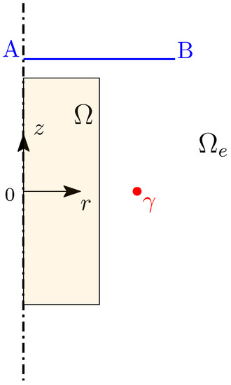
Figure 1. Axisymmetric inductor: a billet (4 cm long and 1 cm radius) is excited by a current loop $\gamma$ (1.5 cm radius and 1000 A); the magnetic flux density was computed along line AB ($0\le r\le 3$ cm and $z=2.5$ cm).

The FEM computational domain is the model cross-section, which corresponds to the $y=0$ plane of the full 3D model. In the FEM model, the exterior region is finite and bounded by a 40 cm radius circle—large enough to make FEM truncation error negligible. A triangle mesh (5461 third-order triangles) was refined up to convergence. The full 3D model was considered in the case of the CM-BEM. The coarsest mesh used for the discretization of $\mathsf{\Omega }$ consisted of 25,157 tetrahedra, 51,282 triangles (1936 of which were on the boundary), 30,863 edges, and 4739 nodes. The mesh was refined in order to obtain a mesh size (i.e., 2.83 mm) smaller than the skin depth of the conductor (7.11 mm at 100 Hz). The eddy-current problem in $\mathsf{\Omega }$ was discretized by using the $a,v$-q formulation with 35,602 DOFs for the CM domain ($a,v$ variables) and 1936 DOFs for the BEM domain (q variables).

To assess the error introduced by matrix compression, the $a,v$-q formulation was implemented: (1) without matrix compression of BEM matrices, (2) with ACA matrix compression, and (3) with R-SVD matrix compression. For case (1), by using the mesh described above, the preprocessing time was 8.37 s, including the construction of CM and BEM matrices of the final linear system, where the latter took most of the time (6.96 s). The solution of the final linear system encompassed the construction of Symmetric Successive Over-Relaxation (SSOR) preconditioner, 0.86 s, and the solution by TFQMR solver, 10.64 s. In this case, the prescribed tolerance of 10⁻¹⁰ was attained in 153 iterations. For case (2), on the same mesh, the corresponding computation times (shown in line 1, Table 1) were: 0.63 for preprocessing, 1.77 s for ACA compression, 0.44 s for preconditioning, and 3.37 s for the TFQMR iterative solution. Finally, for case (3), with R-SVD matrix compression, computation times (shown in line 1, Table 2) were comparable to those of case (2). It can be noted that the preprocessing time for cases (2) and (3) is much less than that for case (1) because the BEM matrices were not explicitly constructed but stored in $\mathcal{H}$-matrix format, by using the same mesh octree with two levels. Moreover, the time required for the construction of the sparse SSOR preconditioner was comparable to that of case (1), while the solution time was almost one third using compressed matrices. It is interesting to note that the same number of iterations (153) and the same smooth convergence pattern were obtained in all three cases, showing that matrix compression does not affect the solver performance. Figure 2 shows the convergence pattern of the TFQMR solver with SSOR preconditioning for case (3).

Table 1. Computation times for the CM-BEM software with ACA compression (prepro: preprocessing, comp: matrix compression, precon: SSOR preconditioner assembly, and sol: TFQMR solver).

# Tets	# DOFs CM/BEM	# Octree Levels	Prepro (s)	ACA Comp (s)	Precon (s)	Sol (s)
25,157	35,602/1936	2	0.63	1.77	0.44	3.37
76,438	106,243/4100	2	2.09	5.44	1.27	17.11
418,089	570,494/12,332	3	13.02	67.00	9.12	140.70
1,735,096	2,346,891/31,132	4	62.09	1684.45	117.41	809.40

Table 2. Computation times for the CM-BEM software with R-SVD compression (prepro: preprocessing, comp: matrix compression, precon: SSOR preconditioner assembly, and sol: TFQMR solver).

# Tets	# DOFs CM/BEM	# Octree Levels	Prepro (s)	R-SVD Comp (s)	Precon (s)	Sol (s)
25,157	35,602/1936	2	0.74	1.42	0.42	3.34
76,438	106,243/4100	2	2.02	4.98	1.25	16.89
418,089	570,494/12,332	3	12.89	41.28	9.08	129.98
1,735,096	2,346,891/31,132	4	64.12	419	119.57	769.34

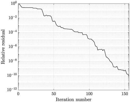
Figure 2. Convergence pattern of the TFQMR solver with SSOR preconditioning at 100 Hz (CM-BEM software with R-SVD compression; coarsest mesh: 25,157 tets).

In order to compare the matrix-compression capabilities of ACA and R-SVD algorithms, four different mesh refinements were considered. The number of octree levels was increased from two (coarsest mesh) to four (finest mesh) in order to reduce the memory usage for BEM matrices and, thus, to make solution feasible also for large-scale problems. Table 1 shows that, for the finest mesh (1,735,096 tetrahedra), the computation time for the construction of $\mathcal{H}$-matrices with ACA is almost four times larger than that with R-SVD, as reported in Table 2, proving the effectiveness of the proposed compression technique. Moreover, it can be noted that the solution times are not affected by the algorithm-type used for compression, while the preprocessing and preconditioning assembly computation times are almost the same because both tasks were performed by using the same code.

The compression ratio for single-layer and double-layer BEM matrices, which are dense and need to be sparsified, is defined as:

$$r\left(\mathbf{M}\right)=1-\frac{\rho \left(\widehat{\mathbf{M}}\right)}{\rho \left(\mathbf{M}\right)},$$

(55)

where the operator $\rho$ indicates the allocated memory, and $\mathbf{M}$, $\widehat{\mathbf{M}}$ are the dense matrix and its corresponding $\mathcal{H}$-matrix, respectively. The definition (55) shows that the ideal compression ($r_{\mathbf{M}}=1$) is obtained when the memory allocated for $\widehat{\mathbf{M}}$ is negligible compared to that of $\mathbf{M}$. Table 3, for the ACA algorithm, and Table 4, for the R-SVD algorithm, show that the compression ratio increases as the number of mesh elements and the number of octree levels increase.

Table 3. Compression ratio of single-layer matrix ${\mathbf{K}}_{\Gamma }$ and double-layer matrix ${\mathbf{V}}_{\Gamma }$ with ACA.

# Tets	Matrix Size	Memory (MB)	# Octree Levels	$\mathit{r}\left({\mathbf{K}}_{\Gamma }\right)$	$\mathit{r}\left({\mathbf{V}}_{\Gamma }\right)$
25,157	1936	28.59	2	35.60%	33.53%
76,438	4100	128.25	2	39.83%	38.90%
418,089	12,332	1160.26	3	82.79%	81.14%
1,735,096	31,132	7394.42	4	93.28%	91.53%

Table 4. Compression ratio of single-layer matrix ${\mathbf{K}}_{\Gamma }$ and double-layer matrix ${\mathbf{V}}_{\Gamma }$ with R-SVD.

# Tets	Matrix Size	Memory (MB)	# Octree Levels	$\mathit{r}\left({\mathbf{K}}_{\Gamma }\right)$	$\mathit{r}\left({\mathbf{V}}_{\Gamma }\right)$
25,157	1936	28.59	2	37.51%	36.08%
76,438	4100	128.25	2	40.84%	40.17%
418,089	12,332	1160.26	3	84.65%	83.88%
1,735,096	31,132	7394.42	4	94.55%	93.80%

In particular, R-SVD shows slightly better compression capabilities along with much smaller computation times (Table 2). It has to be noted that the case with the finest mesh (1,735,096 elements) was intractable without compression since the laptop used for the simulations was equipped with 16 GB RAM. These numerical experiments show that the double-layer matrix (obtained from the analytical-numerical calculation of a non-smooth integral kernel) can also be compressed by using the same ACA (or R-SVD) algorithm used for the single-layer matrix, for which convergence has been theoretically proven [26].

In the compression of single- and double-layer matrices with ACA and R-SVD, the approximation tolerance $\tau$ was set to ${10}^{-3}$. Due to the high computational cost to calculate ${\mathbf{Z}}_{IJ}$, traditional ACA typically makes use of an error estimator, which provides only a rough approximation of (54). This is not required by the R-SVD algorithm, which is not based on an iterative procedure. Figure 3 shows the distribution of compression error (54) for ${\mathbf{V}}_{\Gamma }$, computed by using either ACA or R-SVD. In this histogram, $n_{Z_{IJ}}$ indicates the error count, i.e., the number of submatrices in the $\mathcal{H}$-structure that are in a specific error interval. It can be observed in Figure 3 that most of the submatrices are properly compressed by using either ACA or R-SVD with a compression error smaller than $\tau$. This shows that, for the axisymmetric inductor benchmark, the proposed R-SVD algorithm provides an accurate sparse decomposition while ensuring a much smaller compression time compared to ACA.

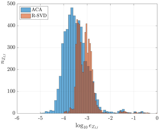
Figure 3. Compression error distribution for the double-layer matrix computed by the ACA and R-SVD algorithms: percentage compression error $e_{Z_{IJ}}$ vs. error count $n_{Z_{IJ}}$. The prescribed tolerance for both algorithms is ${10}^{-3}$, which corresponds to $-3$ in abscissa.

To assess the approximation error produced by matrix compression, numerical results of the CM-BEM software for implementations (1), (2), and (3) were compared with those obtained from third-order 2D FEM. To this end, the magnetic flux density was computed by both CM-BEM and FEM into $N=401$ equally spaced points along the line AB in Figure 1, with the cylindrical coordinates $0\le r\le 3$ cm and $z=2.5$ cm. In particular, the real and imaginary parts of magnetic flux density radial component $B_r$ and axial component $B_z$ were compared. The discrepancy between CM-BEM and FEM values is defined as:

$$\Delta \left(F\right)=\sqrt{\frac{{\sum }_{i=1}^N{\left|F_i-{\overline{F}}_i\right|}^2}{{\sum }_{i=1}^N{\left|{\overline{F}}_i\right|}^2}},$$

(56)

where $F_i$ is the field values computed at the ith point of the line AB by CM-BEM, and ${\overline{F}}_i$ is the reference value computed at the same point by third-order FEM. This definition approximates the $L^2$-norm relative discrepancy along the line AB. The local discrepancy between CM and FEM field values computed at the same points of (56) is defined as:

$$\delta \left(F\right)=\left\{\right|F_i-{\overline{F}}_i|:i=1,\cdots ,N\}.$$

(57)

Even by using the coarsest mesh refinement (25,157 tetrahedra), the discrepancy between third-order FEM (taken as a reference) and CM-BEM was very small. For case (1), without matrix compression, $\Delta \left(\mathrm{R}\mathrm{e}\right(B_r\left)\right)=0.51\%$ for the real part of $B_r$, $\Delta \left(\mathrm{Im}\left(B_r\right)\right)=0.76\%$ for the imaginary part of $B_r$; $\Delta \left(\mathrm{R}\mathrm{e}\right(B_z\left)\right)=0.49\%$ for the real part of $B_z$, $\Delta \left(\mathrm{Im}\left(B_z\right)\right)=0.75\%$ for the imaginary part of $B_z$. Similar results were obtained for case (2) with R-SVD compression: $\Delta \left(\mathrm{R}\mathrm{e}\right(B_r\left)\right)=0.51\%$, $\Delta \left(\mathrm{Im}\left(B_r\right)\right)=0.74\%$, $\Delta \left(\mathrm{R}\mathrm{e}\right(B_z\left)\right)=0.47\%$, $\Delta \left(\mathrm{Im}\left(B_z\right)\right)=0.72\%$. Therefore, accuracy is preserved even after the matrix compression of BEM matrices.

Table 5 and Table 6 show that the discrepancies obtained with ACA and R-SVD algorithms are comparable and decrease as the number of mesh elements increases. Figure 4 and Figure 5 show that the real part and the imaginary part of either $B_r$ or $B_z$, computed by using CM-BEM with R-SVD are in very good agreement with the corresponding second-order FEM profiles. Similar results were obtained by using CM-BEM with ACA matrix compression. Figure 6 and Figure 7 show the local discrepancies computed by (57) when considering field profiles plotted in Figure 4 and Figure 5, respectively.

Table 5. Discrepancy between 3D CM–BEM with ACA compression and third ord. 2D FEM.

# Tets	$\mathsf{\Delta }\left(Re\right({\mathit{B}}_{\mathit{r}}\left)\right)$	$\mathsf{\Delta }\left(\mathbf{Im}\left({\mathit{B}}_{\mathit{r}}\right)\right)$	$\mathsf{\Delta }\left(Re\right({\mathit{B}}_{\mathit{z}}\left)\right)$	$\mathsf{\Delta }\left(\mathbf{Im}\left({\mathit{B}}_{\mathit{z}}\right)\right)$
25,157	0.53%	0.76%	0.49%	0.75%
76,438	0.27%	0.39%	0.28%	0.37%
418,089	0.13%	0.20%	0.16%	0.21%
1,735,096	0.07%	0.12%	0.11%	0.13%

Table 6. Discrepancy between 3D CM–BEM with R-SVD compression and third ord. 2D FEM.

# Tets	$\mathsf{\Delta }\left(Re\right({\mathit{B}}_{\mathit{r}}\left)\right)$	$\mathsf{\Delta }\left(\mathbf{Im}\left({\mathit{B}}_{\mathit{r}}\right)\right)$	$\mathsf{\Delta }\left(Re\right({\mathit{B}}_{\mathit{z}}\left)\right)$	$\mathsf{\Delta }\left(\mathbf{Im}\left({\mathit{B}}_{\mathit{z}}\right)\right)$
25,157	0.51%	0.74%	0.47%	0.72%
76,438	0.27%	0.41%	0.28%	0.41%
418,089	0.13%	0.19%	0.16%	0.20%
1,735,096	0.07%	0.11%	0.11%	0.13%

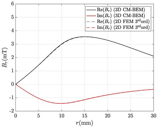
Figure 4. Real and imaginary parts of the magnetic flux density radial component $B_r$ along line A–B depicted in Figure 1 computed by the hybrid method with R-SVD matrix compression: CM-BEM is the straight line, third ord. 2D FEM (reference) is the dashed line.

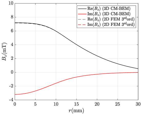
Figure 5. Real and imaginary parts of the magnetic flux density radial component $B_z$ along line A–B depicted in Figure 1 computed by the hybrid method with R-SVD matrix compression: CM-BEM is the straight line, third ord. 2D FEM (reference) is the dashed line.

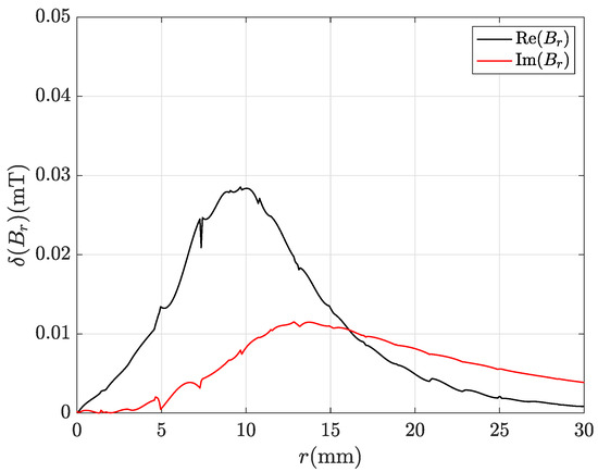
Figure 6. Local discrepancy between CM-BEM and FEM profiles of component $B_r$ in Figure 4.

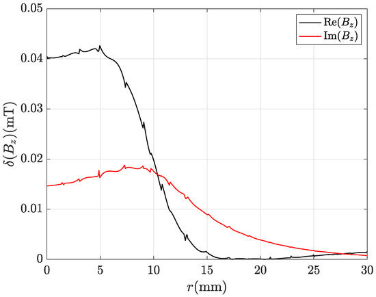
Figure 7. Local discrepancy between CM-BEM and FEM profiles of component $B_z$ in Figure 5.

5.2. TEAM 3 Problem

The following benchmark is useful to show that the hybrid approach with matrix compression can be applied even to 3D models with multiply-connected domains with general topology. As an example, the TEAM 3 Problem (already used in [8] for validating both hybrid a-$\phi$ direct and indirect formulations with dense BEM matrices) is considered here. This benchmark is a classic eddy-current problem used in the literature for validating electromagnetic formulations (see [28] for a detailed description). It consists of an aluminum plate $\mathsf{\Omega }$ (6.35 × 60 × 110 mm, $\sigma =32.78$ MS/m, and ${\mu }_r=1$) with two symmetric holes, excited by a current-driven cylindrical coil ${\mathsf{\Omega }}_0$ (20 mm × 20 mm cross-section, and 20 mm inner radius) carrying 1240 A RMS current at 200 Hz (Figure 8).

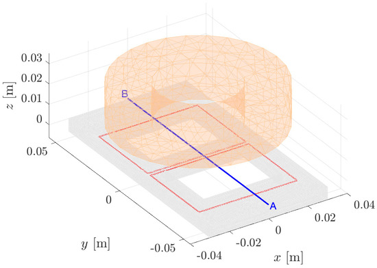
Figure 8. TEAM 3 Problem: an aluminum plate with two symmetric holes excited by current driven coil (orange); virtual loops are depicted in red and the field calculation line AB is depicted in blue.

The case at the smallest frequency (50 Hz) described in the original formulation of the benchmark is not considered here, since it is less stringent for the application of ACA, whose performance deteriorates as the frequency increases as noted in [11]. $\mathsf{\Omega }$ is multiply-connected, with the first Betti number ${\beta }_1=2$. The origin of Cartesian coordinate system $(x,y,z)$ is located at the center of plate top surface. The coil is centered on the plate z vertical axis, 15 mm above the plate. To properly represent the magnetic field in the unbounded air domain ${\mathsf{\Omega }}_e$, virtual loops are introduced in the model geometry (50 × 38 mm rectangular coils), which are depicted as a red line in Figure 8.

For the sake of comparison, the magnetic flux density distribution (real and imaginary parts) was computed by using both 3D CM-BEM and second-order 3D FEM along the line AB with coordinates $x=0$, $-55\le y\le 55$ mm, $z=0.5$ mm (which is depicted in blue in Figure 8). In the FEM model, which also includes the air region, only half geometry is considered due to symmetry (for details, see [8]). The air region of the FEM model is bounded by a parallelepiped of dimensions 0.5 × 0.5 × 1 m—large enough to minimize the truncation error typical of the FEM when homogeneous Neumann boundary conditions at finite distance were applied. The FEM mesh was refined up to convergence: 80,862 second-order tetrahedra were used in the whole domain, corresponding to 517,341 DOFs; the TFQMR solver with multigrid preconditioner attained the ${10}^{-12}$ relative tolerance in 48 s.

The same numerical tests as in the axisymmetric inductor benchmark were performed. The initial mesh refinement was constructed in order to properly capture the skin effect at 200 Hz frequency: it consisted of 69,492 tetrahedra, 143,798 triangles (9628 of which were located on the plate boundary), 88,443 edges, and 14,136 nodes. In such a way, the mesh size (1.45 mm) was smaller than the skin depth (6.22 mm) at the operating frequency. The eddy-current problem in $\mathsf{\Omega }$ was discretized by using the $a,v$-q formulation (only with matrix compression). For the initial mesh refinement, 102,579 DOFs for the CM domain ($a,v$ variables) and 9628 DOFs (q variables) for the BEM domain were used. Two additional DOFs were required to properly represent the magnetic field in ${\mathsf{\Omega }}_e$ because ${\beta }_1=2$. Thus, the algebraic structure of the linear system was different from the simply connected case, and the convergence properties had to be checked again. Moreover, it has to be noted that, for this benchmark, even with a rather coarse mesh (69,492 elements), it was not possible to use the $a,v$-q formulation without matrix compression due to the excessive amount of memory required by dense off-diagonal matrix blocks in (51).

The following scenarios were considered for the hybrid approach: (1) with ACA matrix compression and (2) with R-SVD matrix compression. For case (1), the corresponding computation times (reported in Table 7) were: 101.39 s for preprocessing, 82.54 s for ACA compression, 4.50 s for preconditioning, and 21.71 s for the TFQMR iterative solution. In this case, the ${10}^{-10}$ tolerance was attained in 208 iterations. For case (2), unlike the inductor benchmark, the R-SVD compression allowed in this case for a considerable computation time reduction compared to case (1). In fact, it can be noted in Table 8 that only 25.49 s (almost one third of ACA) were needed for R-SVD compression. The same number of iterations as case (1) was achieved by the TFQMR solver with a smooth convergence pattern (Figure 9). These results show that the convergence behavior of the $a,v$-q formulation does not depend on the type of algorithm used for matrix compression.

Table 7. Computation times for the CM-BEM software with ACA compression (prepro: preprocessing, comp: matrix compression, precon: SSOR preconditioner assembly, and sol: TFQMR solver).

# Tets	# DOFs CM/BEM	# Octree Levels	Prepro (s)	ACA Comp (s)	Precon (s)	Sol (s)
69,492	102,579/9628	5	101.39	82.54	4.50	21.71
105,481	153,422/12,508	5	122.45	96.81	7.59	38.50
248,427	352,526/20,912	5	206.42	135.69	28.42	95.56
435,213	610,778/30,316	5	316.17	285.26	73.16	171.39

Table 8. Computation times for the CM-BEM software with R-SVD compression (prepro: preprocessing, comp: matrix compression, precon: SSOR preconditioner assembly, and sol: TFQMR solver).

# Tets	# DOFs CM/BEM	# Octree Levels	Prepro (s)	R-SVD Comp (s)	Precon (s)	Sol (s)
69,492	102,579/9628	5	99.31	25.49	4.36	19.81
105,481	153,422/12,508	5	124.32	32.88	7.77	33.08
248,427	352,526/20,912	5	208.75	58.26	28.70	93.39
435,213	610,778/30,316	5	314.30	93.45	72.66	181.12

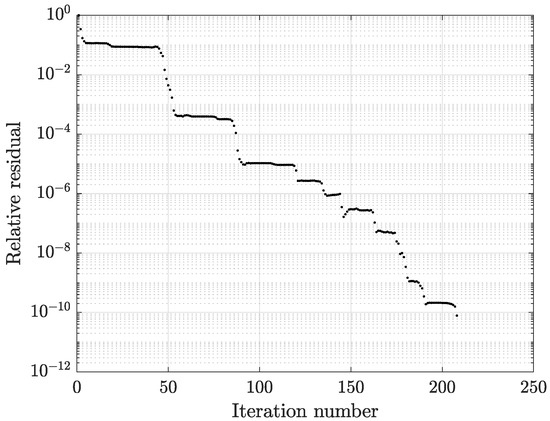
Figure 9. Convergence pattern of the TFQMR solver with SSOR preconditioning at 200 Hz (CM-BEM software with R-SVD compression, coarsest mesh: 69,492 tets).

In order to compare the matrix-compression capabilities of ACA and R-SVD algorithms, four different mesh refinements were used. Five levels were taken for the construction of octree need for $\mathcal{H}$-matrices, in order to obtain a good trade-off between memory occupation and computation time required for matrix compression. By comparing the computation times needed by ACA and R-SVD for different discretizations (Table 7 and Table 8), it can be observed that R-SVD algorithm is much faster (i.e., only one-third of the ACA time is needed). This proves the effectiveness of the proposed compression algorithm. The other computation times (preprocessing, preconditioning, and TFQMR solution) are almost unchanged because the same code was used for these tasks.

Table 9 shows that compression ratios of the CM-BEM with ACA are lower than those of the CM-BEM with R-SVD as given in Table 10. The compression ratio increases as the number of elements increases for both ACA and R-SVD algorithms. By using an octree with five levels for the $\mathcal{H}$-matrix generation the compression ratio becomes very high (around 90%). It can be noted that, when the finest mesh is considered (435,213 tetrahedra), single- and double-layer matrices cannot be stored without matrix compression on a standard laptop equipped with 16 GB RAM. These numerical experiments show that double-layer matrix can be compressed as well by using the same ACA (or R-SVD) algorithm used for the single-layer matrix.

Table 9. Compression ratio of single-layer matrix ${\mathbf{K}}_{\Gamma }$ and double-layer matrix ${\mathbf{V}}_{\Gamma }$ with ACA.

Mesh	Matrix Size	Memory (MB)	# Octree Levels	$\mathit{r}\left({\mathbf{K}}_{\Gamma }\right)$	$\mathit{r}\left({\mathbf{V}}_{\Gamma }\right)$
69,492	9628	707.23	5	87.56%	84.52%
105,481	12,508	1193.62	5	90.28%	87.91%
248,427	20,912	3336.42	5	93.67%	92.22%
435,213	30,316	7011.87	5	95.18%	94.11%

Table 10. Compression ratio of single-layer matrix ${\mathbf{K}}_{\Gamma }$ and double-layer matrix ${\mathbf{V}}_{\Gamma }$ with R-SVD.

Mesh	Matrix Size	Memory (MB)	# Octree Levels	$\mathit{r}\left({\mathbf{K}}_{\Gamma }\right)$	$\mathit{r}\left({\mathbf{V}}_{\Gamma }\right)$
69,492	9628	707.23	5	90.37%	88.08%
105,481	12,508	1193.62	5	92.57%	90.76%
248,427	20,912	3336.42	5	95.12%	94.03%
435,213	30,316	7011.87	5	96.19%	95.43%

The effectiveness of both compression algorithms is examined again by considering the compression error (54), which evaluates the accuracy of low-rank sub-block approximations in the $\mathcal{H}$-matrix. By setting the threshold value $\tau$ as usual to ${10}^{-3}$ for both ACA and R-SVD, it can be noted in Figure 10 that ACA is not accurate since most of error occurrences are above $\tau$. This shows that ACA is ineffective for the compression of the double-layer matrix. It is also not robust since its performance depends on the type of model geometry (i.e., ACA works for the axysimmetric inductor model but not for the TEAM 3 model). In contrast, R-SVD provides an accurate sparse approximation and it is also robust for both models.

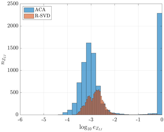
Figure 10. Compression error distribution for the double-layer matrix computed by ACA and R-SVD algorithms: percentage compression error $e_{Z_{IJ}}$ vs. error count $n_{Z_{IJ}}$. The prescribed tolerance for both algorithms is ${10}^{-3}$, which corresponds to $-3$ in abscissa.

It can be observed that such inaccuracy of the ACA in matrix compression leads to an inaccurate solution of the field problem. To show this issue, real and imaginary parts of the magnetic flux density components along $y,z$ axes were computed on equally spaced 401 points, along the line AB in Figure 8. In Table 11, it can be observed that, by increasing the number of mesh elements the discrepancy from the reference field distribution (obtained with second-order 3D FEM) increases as well. On the contrary, this loss in accuracy is not present in simulations obtained by the CM-BEM with R-SVD compression (see Table 12).

Table 11. Discrepancy between 3D CM–BEM with ACA compression and second order 3D FEM.

# Tets	$\mathbf{\Delta }\left(Re\right({\mathit{B}}_{\mathit{y}}\left)\right)$	$\mathbf{\Delta }\left(\mathbf{Im}\left({\mathit{B}}_{\mathit{y}}\right)\right)$	$\mathbf{\Delta }\left(Re\right({\mathit{B}}_{\mathit{z}}\left)\right)$	$\mathbf{\Delta }\left(\mathbf{Im}\left({\mathit{B}}_{\mathit{z}}\right)\right)$
69,492	1.56%	5.89%	1.98%	5.28%
105,481	2.19%	8.27%	3.05%	8.05%
248,427	2.53%	9.88%	3.41%	9.46%
435,213	3.03%	11.02%	4.26%	10.81%

Table 12. Discrepancy between 3D CM–BEM with R-SVD compression and second order 3D FEM.

# Tets	$\mathbf{\Delta }\left(Re\right({\mathit{B}}_{\mathit{y}}\left)\right)$	$\mathbf{\Delta }\left(\mathbf{Im}\left({\mathit{B}}_{\mathit{y}}\right)\right)$	$\mathbf{\Delta }\left(Re\right({\mathit{B}}_{\mathit{z}}\left)\right)$	$\mathbf{\Delta }\left(\mathbf{Im}\left({\mathit{B}}_{\mathit{z}}\right)\right)$
69,492	1.24%	4.74%	1.50%	4.82%
105,481	1.05%	4.56%	1.27%	4.73%
248,427	0.77%	4.36%	0.82%	4.55%
435,213	0.70%	4.37%	0.72%	4.61%

Even by using the coarsest mesh refinement (69,492 tetrahedra), numerical results of CM-BEM with R-SVD matrix compression (case 2) are in good agreement with second-order FEM taken as a reference. Figure 11 and Figure 12 show that real and imaginary parts of either $B_y$ or $B_z$, computed by using CM-BEM with R-SVD matrix compression, are in very good agreement with the corresponding second-order FEM values. Figure 13 and Figure 14 show the corresponding local discrepancy profiles computed by (57). In particular, the discrepancies computed by (56) are: $\Delta \left(\mathrm{R}\mathrm{e}\right(B_y\left)\right)=1.24\%$, $\Delta \left(\mathrm{Im}\left(B_y\right)\right)=4.74\%$ for $B_y$ component; $\Delta \left(\mathrm{R}\mathrm{e}\right(B_z\left)\right)=1.50\%$, $\Delta \left(\mathrm{Im}\left(B_z\right)\right)=4.82\%$ for $B_z$ component. Moreover, it can be observed in Table 12 that the discrepancy decreases as the number of mesh elements increases. The imaginary part shows a larger discrepancy compared to the real part because since the imaginary part is ten-times smaller. In contrast, results from the CM-BEM with ACA matrix compression show that this approach is not reliable since it is not convergent, i.e., the discrepancy of $B_z$ imaginary part increases as the number of mesh elements increases (Table 11).

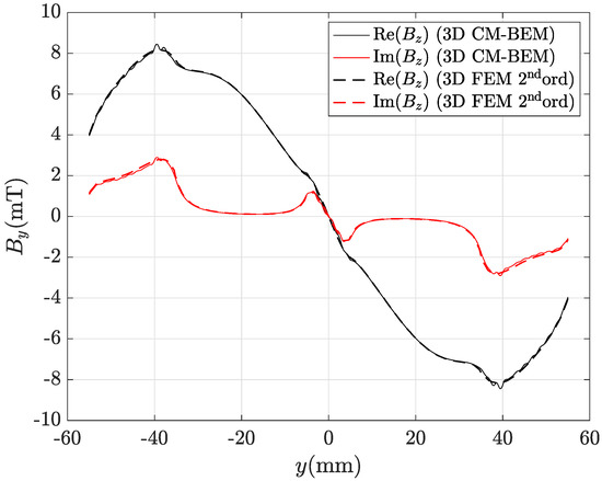
Figure 11. Real and imaginary parts of the magnetic flux density radial component $B_y$ along line AB in Figure 8 computed by the hybrid method (R-SVD matrix compression) with the coarsest mesh (69,492 tets): CM-BEM is the straight line, second ord. 3D FEM (reference) is the dashed line.

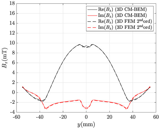
Figure 12. Real and imaginary parts of the magnetic flux density radial component $B_z$ along line AB depicted in Figure 8 computed by the hybrid method (R-SVD matrix compression) with the coarsest mesh (69,492 tets): CM-BEM is the straight line, second ord. 3D FEM (reference) is the dashed line.

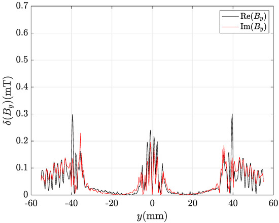
Figure 13. Local discrepancy between CM-BEM and FEM profiles of component $B_y$ in Figure 11.

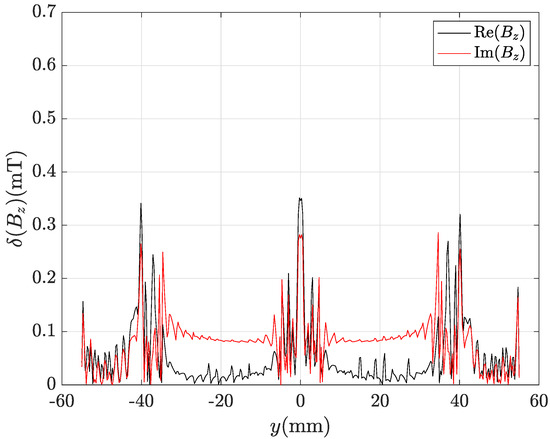
Figure 14. Computed byLocal discrepancy between CM-BEM and FEM profiles of component $B_z$ in Figure 12.

Even by using the finest mesh refinement (435,213 tetrahedra), the CM-BEM with ACA matrix compression provides incorrect results as can be observed from profiles of $B_y$, $B_z$ real and imaginary parts shown in Figure 15 and Figure 16. Figure 17 and Figure 18 show the corresponding local discrepancy profiles. In particular, it can be noted that around $y=\pm 40$ mm is almost doubled compared to the corresponding plots for CM-BEM with R-SVD (Figure 13 and Figure 14). The discrepancies computed by (56) are: $\Delta \left(\mathrm{R}\mathrm{e}\right(B_y\left)\right)=3.03\%$, $\Delta \left(\mathrm{Im}\left(B_y\right)\right)=11.02\%$ for $B_y$ component; $\Delta \left(\mathrm{R}\mathrm{e}\right(B_z\left)\right)=4.26\%$, $\Delta \left(\mathrm{Im}\left(B_z\right)\right)=10.81\%$ for $B_z$ component. These values are much higher than those shown above for CM-BEM with R-SVD.

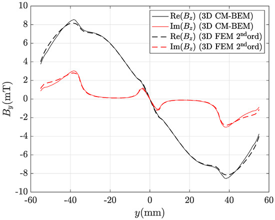
Figure 15. Real and imaginary parts of the magnetic flux density radial component $B_y$ along line AB in Figure 8 computed by the hybrid method (ACA matrix compression) with the finest mesh (435,213 tets): CM-BEM is the straight line, second ord. 3D FEM (reference) is the dashed line.

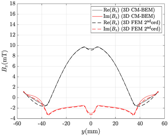
Figure 16. Real and imaginary parts of the magnetic flux density radial component $B_z$ along line AB depicted in Figure 8 computed by the hybrid method (ACA matrix compression) with the finest mesh (435,213 tets): CM-BEM is the straight line, second ord. 3D FEM (reference) is the dashed line.

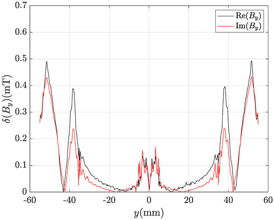
Figure 17. Local discrepancy between CM-BEM and FEM profiles of component $B_y$ in Figure 15.

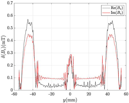
Figure 18. Local discrepancy between CM-BEM and FEM profiles of component $B_z$ in Figure 16.

The TEAM 3 model was also simulated using FEM to compare the performance of a state-of-the-art method with that of the proposed hybrid method. A MATLAB^® vectorized implementation of the standard A, V–A formulation (typically adopted in FEM commercial software for electromagnetic analysis) was performed. The implementation is based on use of edge and face Whitney elements for discretization (these are vector basis functions described, e.g., in [29]), and on the numerical treatment of the RHS proposed in [30], which ensures a good convergence behavior of Krylov iterative solvers. The final system of linear equations is complex symmetric and was solved by the same solver used for CM-BEM (i.e., TFQMR + SSOR preconditioner).

For a fair comparison, first-order FEM was considered (which corresponds to a pure CM) and the FEM mesh in the plate was generated with a number of tetrahedra similar to that of the CM-BEM. In this way, approximately the same number of DOFs was used by pure FEM and CM-BEM model (which includes only the discretization of the plate). The air region was bounded by a cube of the 1 m side, as the parallelepiped used for the second-order FEM model. To ensure a good transition of the mesh between the conductive region and the air region, and thus a reliable solution, a large number of tetrahedra was required with the FEM, which led, in turn, to a large number of DOFs.

To compare the computational performance of the FEM with respect to that of the CM-BEM with R-SVD compression (see computation times in Table 8), four different mesh refinements, with a number of tetrahedra similar to that of the CM-BEM models, were considered. Figure 19 shows the FEM mesh distribution near the plate and the coil for the first examined model with the coarsest mesh refinement (69,702 tets for plate, 1,171,167 tets for air): many elements were required to ensure a good transition of the mesh from the conductive region to the air region.

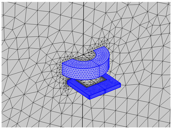
Figure 19. Distribution of the FEM mesh near the plate and the coil, whose elements are depicted in blue (coarsest case: 69,702 tets for plate and 1,171,167 tets for air): element size within the plate has to be smaller than skin depth; many elements have to be used in the air region to ensure a good transition.

For this discretization, the computation times for preprocessing (i.e., the assembly of FEM matrices and RHS, and the numerical treatment of the coil), SSOR preconditioning, and solution were 148.73 s, 67.93 s, and 148.56 s, respectively (Table 13). It can be observed that the solution time for the FEM is at least seven times greater than that required by the CM-BEM with R-SVD matrix compression (Table 8), which clearly shows the validity of the proposed method. The same consideration holds also when refining the mesh: computation times in Table 13, for the FEM, are much greater than those in Table 8, for the CM-BEM.

Table 13. Computation times for first ord. FEM software implementing the A, V-A formulation (prepro: preprocessing, comp: matrix compression, precon: SSOR preconditioner assembly, and sol: TFQMR solver).

# Tets Plate	# Tets Air	# DOFs FEM	Prepro (s)	Precon (s)	Sol (s)
69,702	1.171,167	1,500,258	148.73	67.93	148.56
105,384	1,706,681	2,178,508	232.42	127.38	271.33
248,174	2,300,615	3,067,714	337.43	270.50	463.64
433,737	3,157,965	4,323,418	519.17	429.78	772.48

Concerning the FEM solution, the number of TFQMR iterations to attain the solver prescribed tolerance of ${10}^{-10}$ was almost doubled compared to the CM-BEM: for the coarsest case, the solver converged into 372 iterations instead of 208 of the CM-BEM. Figure 20 shows the convergence pattern of the TFQMR + SSOR solver for the FEM, which corresponds to Figure 9 evaluated for the same solver when running the CM-BEM model.

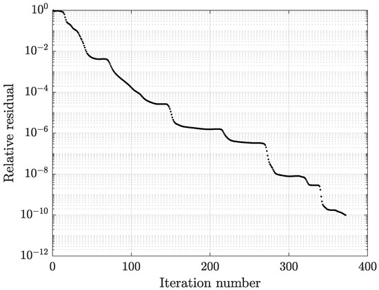
Figure 20. Convergence pattern of the TFQMR solver with SSOR preconditioning at 200 Hz (first ord. 3D FEM with coarsest mesh: 69,702 tets for plate, 1,171,167 tets for air).

Finally, despite the large number of tetrahedra used in the air region, it can be noted that first-order FEM is not very accurate. Figure 21 and Figure 22 show that FEM profiles are very irregular and differ from those of second-order FEM, which are very smooth, such as those of the CM-BEM. In particular, the discrepancies computed by (56) are: $\Delta \left(\mathrm{R}\mathrm{e}\right(B_y\left)\right)=11.93\%$, $\Delta \left(\mathrm{Im}\left(B_y\right)\right)=9.98\%$ for $B_y$ component; $\Delta \left(\mathrm{R}\mathrm{e}\right(B_z\left)\right)=14.19\%$, $\Delta \left(\mathrm{Im}\left(B_z\right)\right)=12.18\%$ for $B_z$ component. These values are much greater than those of the CM-BEM with R-SVD compression for a mesh in the plate of comparable size (Table 12).

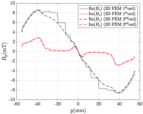
Figure 21. Real and imaginary parts of the magnetic flux density radial component $B_y$ along line AB depicted in Figure 8 computed by FEM with the coarsest mesh (69,702 tets for plate, 1,171,167 tets for air): first ord. 3D FEM is the straight line, second ord. 3D FEM (reference) is the dashed line.

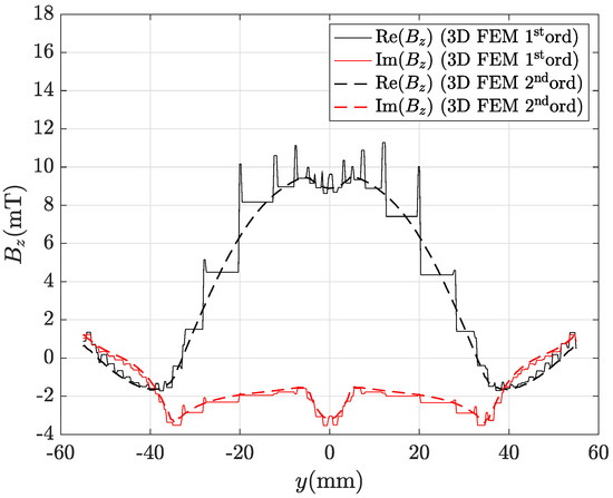
Figure 22. Real and imaginary parts of the magnetic flux density radial component $B_z$ along line AB depicted in Figure 8 computed by FEM with the coarsest mesh (69,702 tets for plate, 1,171,167 tets for air): first ord. 3D FEM is the straight line, second ord. 3D FEM (reference) is the dashed line.

6. Conclusions

We proposed a novel hybrid method for the analysis of time-harmonic eddy-current problems. This method was coupled to a novel R-SVD matrix-compression technique to reduce both the assembly time and the amount of allocated memory needed for BEM matrices. As a result, the simulation of large-scale unbounded field problems becomes feasible even on a standard laptop at a reasonable computational cost. Numerical examples show that the R-SVD algorithm is more accurate, faster and more robust than the classical ACA algorithm when applied to the compression of BEM matrices.

A comparison with first-order FEM also shows that the CM-BEM provides much higher performance in terms of computation time due to a much smaller number of DOFs. Furthermore, when analyzing a test case of engineering interest, the CM-BEM with R-SVD matrix compression shows very good agreement with high-order FEM although the former uses much fewer degrees of freedom.

References

- Tonti, E. Finite Formulation of the Electromagnetic Field. Prog. Electromagn. Res. 2001, 32, 1–44. [Google Scholar] [CrossRef]
- Giuffrida, C.; Gruosso, G.; Repetto, M. Finite formulation of nonlinear magnetostatics with Integral boundary conditions. IEEE Trans. Magn. 2006, 42, 1503–1511. [Google Scholar] [CrossRef]
- Codecasa, L.; Minerva, V.; Politi, M. Use of barycentric dual grids for the solution of frequency domain problems by FIT. IEEE Trans. Magn. 2004, 40, 1414–1419. [Google Scholar] [CrossRef]
- Codecasa, L.; Trevisan, F. Constitutive equations for discrete electromagnetic problems over polyhedral grids. J. Comput. Phys. 2007, 225, 1894–1918. [Google Scholar] [CrossRef]
- Moro, F.; Codecasa, L. Indirect Coupling of the Cell Method and BEM for Solving 3-D Unbounded Magnetostatic Problems. IEEE Trans. Magn. 2016, 52, 1–4. [Google Scholar] [CrossRef]
- Moro, F.; Codecasa, L. A 3-D Hybrid Cell Method for Induction Heating Problems. IEEE Trans. Magn. 2017, 53, 1–4. [Google Scholar] [CrossRef]
- Moro, F.; Codecasa, L. A 3-D Hybrid Cell Boundary Element Method for Time-Harmonic Eddy Current Problems on Multiply Connected Domains. IEEE Trans. Magn. 2019, 55, 1–11. [Google Scholar] [CrossRef]
- Moro, F.; Codecasa, L. Coupling the Cell Method with the Boundary Element Method in Static and Quasi–Static Electromagnetic Problems. Mathematics 2021, 9, 1426. [Google Scholar] [CrossRef]
- Codecasa, L. Refoundation of the Cell Method Using Augmented Dual Grids. IEEE Trans. Magn. 2014, 50, 497–500. [Google Scholar] [CrossRef]
- Bebendorf, M. Approximation of boundary element matrices. Numer. Math. 2000, 86, 565–589. [Google Scholar] [CrossRef]
- Lahaye, D.; Tang, J.; Vuik, K. Modern Solvers For Helmholtz Problems; Birkhäuser: Basel, Switzerland, 2017. [Google Scholar]
- Alotto, P.; Bettini, P.; Specogna, R. Sparsification of BEM Matrices for Large-Scale Eddy Current Problems. IEEE Trans. Magn. 2016, 52, 1–4. [Google Scholar] [CrossRef]
- Echeverri Bautista, M.A.; Francavilla, M.A.; Vipiana, F.; Vecchi, G. A Hierarchical Fast Solver for EFIE-MoM Analysis of Multiscale Structures at Very Low Frequencies. IEEE Trans. Antennas Propag. 2014, 62, 1523–1528. [Google Scholar] [CrossRef]
- Smajic, J.; Andjelic, Z.; Bebendorf, M. Fast BEM for Eddy-Current Problems Using H-Matrices and Adaptive Cross Approximation. Magn. IEEE Trans. 2007, 43, 1269–1272. [Google Scholar] [CrossRef]
- Knittel, A.; Franchin, M.; Bordignon, G.; Fischbacher, T.; Bending, S.; Fangohr, H. Compression of boundary element matrix in micromagnetic simulations. J. Appl. Phys. 2009, 105, 07D542. [Google Scholar] [CrossRef]
- Hertel, R.; Christophersen, S.; Börm, S. Large-scale magnetostatic field calculation in finite element micromagnetics with H2-matrices. J. Magn. Magn. Mater. 2019, 477, 118–123. [Google Scholar] [CrossRef]
- Bruckner, F.; Vogler, C.; Feischl, M.; Praetorius, D.; Bergmair, B.; Huber, T.; Fuger, M.; Suess, D. 3D FEM–BEM coupling method to solve magnetostatic Maxwell equations. J. Magn. Magn. Mater. 2012, 324, 1862–1866. [Google Scholar] [CrossRef]
- Alonso Rodríguez, A.; Bertolazzi, E.; Ghiloni, R.; Valli, A. Finite element simulation of eddy current problems using magnetic scalar potentials. J. Comput. Phys. 2015, 294, 503–523. [Google Scholar] [CrossRef]
- Munkres, J. Elem. Algebr. Topol.; Perseus Books: New York, NY, USA, 1984. [Google Scholar]
- Gross, P.; Kotiuga, P. Electromagnetic Theory and Computation: A Topological Approach; Cambridge University Press: Cambridge, UK, 2011. [Google Scholar]
- Hiptmair, R.; Sterz, O. Current and voltage excitations for the eddy current model. Int. J. Numer. Model. Electron. Netw. Devices Fields 2005, 18, 1–21. [Google Scholar] [CrossRef]
- Folland, G. Introduction to Partial Differential Equations; Princeton University Press: Princeton, NJ, USA, 1995. [Google Scholar]
- Ostrowski, J.; Andjelic, Z.; Bebendorf, M.; Cranganu-Cretu, B.; Smajic, J. Fast BEM-solution of Laplace problems with H-matrices and ACA. IEEE Trans. Magn. 2006, 42, 627–630. [Google Scholar] [CrossRef]
- Kurz, S.; Rain, O.; Rjasanow, S. The adaptive cross-approximation technique for the 3D boundary-element method. IEEE Trans. Magn. 2002, 38, 421–424. [Google Scholar] [CrossRef]
- Heldring, A.; Ubeda, E.; Rius, J.M. On the Convergence of the ACA Algorithm for Radiation and Scattering Problems. IEEE Trans. Antennas Propag. 2014, 62, 3806–3809. [Google Scholar] [CrossRef]
- Bebendorf, M.; Rjasanow, S. Adaptive Low-Rank Approximation of Collocation Matrices. Computing 2003, 70, 1–24. [Google Scholar] [CrossRef]
- Rius, J.; Tamayo, J.; Heldring, A.; Parrón, J.; Ubeda, E. ACAsolver Software. Available online: https://antennalab.upc.edu/en/acasolver-software (accessed on 2 October 2022).
- International Compumag Society. TEAM 3 Problem: Bath Plate with Two Holes. Available online: https://www.compumag.org/jsite/images/stories/TEAM/problem3.pdf (accessed on 6 October 2022).
- Bossavit, A. Computational Electromagnetism: Variational Formulations, Complementarity, Edge Elements; Academic: New York, NY, USA, 1998. [Google Scholar]
- Ren, Z. Influence of the RHS on the convergence behaviour of the curl–curl equation. IEEE Trans. Magn. 1996, 32, 655–658. [Google Scholar] [CrossRef]
Disclaimer/Publisher’s Note: The statements, opinions and data contained in all publications are solely those of the individual author(s) and contributor(s) and not of MDPI and/or the editor(s). MDPI and/or the editor(s) disclaim responsibility for any injury to people or property resulting from any ideas, methods, instructions or products referred to in the content. |
© 2023 by the authors. Licensee MDPI, Basel, Switzerland. This article is an open access article distributed under the terms and conditions of the Creative Commons Attribution (CC BY) license (https://creativecommons.org/licenses/by/4.0/).