Weighted Competing Risks Quantile Regression Models and Variable Selection

Abstract

The proportional subdistribution hazards (PSH) model is popularly used to deal with competing risks data. Censored quantile regression provides an important supplement as well as variable selection methods due to large numbers of irrelevant covariates in practice. In this paper, we study variable selection procedures based on penalized weighted quantile regression for competing risks models, which is conveniently applied by researchers. Asymptotic properties of the proposed estimators, including consistency and asymptotic normality of non-penalized estimator and consistency of variable selection, are established. Monte Carlo simulation studies are conducted, showing that the proposed methods are considerably stable and efficient. Real data about bone marrow transplant (BMT) are also analyzed to illustrate the application of the proposed procedure.

1. Introduction

In survival analysis, sometimes events fail because of a specific cause or from some other causes or competing risks. Consider the dataset of bone marrow transplant (BMT) in [1] for example, which includes 177 patients who received a stem cell transplant for acute leukemia. Whereas 56 patients in this dataset relapsed (REL), considered as the event of interest, 75 patients died from causes related to the transplant (transplant related mortality, TRM), which is considered a competing risk, as it hinders the occurrence of leukemia relapse. The other 46 patients are regarded as censored due to the end of the study. In the analysis of such a dataset, treating competing risks (TRM) as censoring cases and using usual Cox modelling may be inaccurate, as the competing risks are probably affected by covariates. To deal with such competing risks data, Ref. [2] proposed a novel semiparametric proportional hazards for the subdistribution, or PSH model, which directly analyzes the effect of covariates on the marginal probability function or cumulative incidence function (CIF). The competing risks data often occur in clinical trials containing large numbers of covariates, among which only a few have significant or essential influence on the response, generating the variable selection issues, such as the general penalized log-partial likelihood method proposed by [3].

Quantile regression introduced by [4] is widely known to more comprehensively describe the conditional distribution of response on covariates. Existing work about competing risks quantile regression includes [5], which first transforms competing risks quantile regression models to accelerated the failure model and uses an estimating equation procedure for estimation. In addition, Ref. [6] discussed the quantile regression for competing risks data with missing cause of failure. Then [7,8] developed variable selection procedures based on unbiased estimating equations with group structures and penalization methods for competing risks quantile regression models.

In the paper, in spite of the estimating equation method, we propose developing a more general method for competing risks quantile regression and expanding the weighted procedures by considering the re-distribution methods [9] for the PSH model. By transformed responses, we can rewrite the competing risks quantiles formulation as a general quantile regression objective function, then apply the constructed weights. With unbiasedness of the subgradient of this weighted objective function at the true cumulative-incidence function and coefficient proved, consistency and asymptotic normality of the penalty-free estimators are established under regularity conditions. To realize the variable selection, penalization methods such as the least absolute shrinkage and selection operator (LASSO) proposed by [10] and the adaptive LASSO (ALASSO) developed by [11] are applied to the weighted objective function, which can be easily applied with the R package. The consistency of the variable selection procedure is also established, and Monte Carlo simulation is performed to illustrate the efficiency and stability of our proposed procedures. Real data about bone marrow transplant are analyzed using our methods.

The paper is organized as follows. Our proposed weighted competing risks quantile regression model and its penalized methods are developed in Section 2, with asymptotic properties demonstrated in Section 3. Simulation studies as well as the application to the BMT data are performed in Section 4 to illustrate the performance of proposed methods.

2. Models

We take the formulation of competing risks quantile regression in [5]. In the setting of competing risks models, assume there exist K causes of failure, denoted by an observable indicator $ϵ\in \{1,\dots ,K\}$, the same denotation as [2]. Without loss of generality, we can set $K=2$. Let T and C denote the failure and censoring time, respectively, and we observe $X=min(T,C)$, and censoring or risk indicator $\delta =I(T\le C),$ where $I(·)$ is an indicator function. Denote a $p\times 1$ bounded time-independent covariate vector as $\tilde{Z}$ and $Z={(1,{\tilde{Z}}^{\top })}^{\top }$. Assume that $\{X_i,{\delta }_i{ϵ}_i,Z_i\},i=1,\dots ,n$ are independent and identically distributed observed samples.

Ref. [2] modeled the CIF for failure from cause 1 conditionally on the covariates, $F_1\left(t\right|Z)=P(T\le t,ϵ=1|Z)$. They proposed the PSH model based on the formula of subdistribution hazard, which is defined as

$$\begin{array}{ccc}\hfill {\lambda }_1\left(t\right|Z)& =& \underset{\Delta t\to 0}{lim}\frac{1}{\Delta t}P\left\{t<T\le t+\Delta t,ϵ=1\left|\right(T\ge t)\cup (T\le t\cap ϵ\ne 1),Z\right\}\hfill \\ & =& \{d{F}_1\left(t\right|Z)/dt\}/\{1-F_1\left(t\right|Z)\}\hfill \end{array}$$

in [12]. Analogue to the definition of quantile, we define the conditional quantile as $Q_k\left(\tau \right|Z)=inf\{t:F_k\left(t\right|Z)\ge \tau \},k=1,\dots ,K$, where $F_k\left(t\right|Z)=P\{T\le t,ϵ=k\}$ is the CIF for cause k; for more details, refer to [5]. For $\tau \in [{\tau }_L,{\tau }_U]$, consider $Q_1\left(\tau \right|Z)$ to be modeled as

$$\begin{array}{c}\hfill Q_1\left(\tau \right|Z)=g\left\{Z^{\top }{\beta }_0\left(\tau \right)\right\},\end{array}$$

(1)

where ${\beta }_0\left(\tau \right)$ is a $(p+1)\times 1$ coefficient vector, $g(·)$ is a known monotone increasing and continuously differential bounded link function, $0<{\tau }_L\le {\tau }_U<1$. With the statement in [2], if we denote $T_1^{*}=I(ϵ=1)\times T+\{1-I(ϵ=1)\}\times \infty$, then $T_1^{*}$ has a distribution function equal to $F_1\left(t\right|Z)$ when $t<\infty$ and a point mass $P(T^{*}=\infty |Z)=P(T<\infty ,ϵ\ne 1)=1-F_1(\infty |Z)$ at $t=\infty$. Then, at $\tau <F_1(\infty |Z)$, the $\tau -$quantile of $T_1^{*}$ equals $F_1^{-1}\left(\tau \right|Z)=Q_1\left(\tau \right|Z)=g\left\{Z^{\top }{\beta }_0\left(\tau \right)\right\}$ under the formulation of (1).

Remark 1.

According to the formulation of $T_1^{*}$, we can see that when $\tau \ge F_1(\infty ;Z)$, the $\tau -$quantile of $T_1^{*}$ will become ∞, which is obvious when reviewing the definition that $F_1(t;Z)=P(T\le t,ϵ=1|Z)\le P(T\le \infty ,ϵ=1|Z)=F_1(\infty ;Z)$ and the fact that $g(·)$ is monotone increasing. This fact provides a thought about the choice of ${\tau }_U$.

With reference to [13], for proper $\tau$, ${\beta }_0\left(\tau \right)$ is supposed to be the minimizer of the following expected loss function with respect to $\beta \left(\tau \right)$:

$$\begin{array}{c}\hfill {\beta }_0\left(\tau \right)=arg\underset{\beta \left(\tau \right)}{min}E{\rho }_{\tau }(g^{-1}\left(T_1^{*}\right)-Z^{\top }\beta \left(\tau \right)),\end{array}$$

(2)

where E denotes the expectation, and ${\rho }_{\tau }\left(u\right)=u\{\tau -I(u\le 0)\}$ is called the “check” function.

In a sample scenario, we can obtain the estimator $\widehat{\beta }\left(\tau \right)$ of ${\beta }_0\left(\tau \right)$ via minimizing the following objective function:

$$\begin{array}{c}\hfill \underset{\beta \left(\tau \right)}{min}\sum _{i=1}^n{\rho }_{\tau }\left(g^{-1}\left(T_{1,i}^{*}\right)-Z_i^{\top }\beta \left(\tau \right)\right).\end{array}$$

(3)

2.1. Weighted Competing Risks Quantile Regression

Similar to [5], our paper first considers the case in which there are no missing data (i.e., there is no censoring). As a result, $X=T$ and $\delta =1,\delta ϵ=ϵ$. As aforementioned, we can estimate ${\beta }_0\left(\tau \right)$ via the minimization problem (3). Because $T_{1,i}^{*}$ is not observed, we modify (3) to

$$\begin{array}{c}\hfill \sum _{i=1}^{n}I({ϵ}_i=1){\rho }_{\tau }(g^{-1}\left(X_i\right)-Z_i^{\top }\beta \left(\tau \right))+I({ϵ}_i\ne 1){\rho }_{\tau }(g^{-1}\left(X^{\infty }\right)-Z_i^{\top }\beta \left(\tau \right)),\end{array}$$

(4)

where $X^{\infty }$ is any value sufficiently large to exceed all $Z_i^{\top }\beta \left(\tau \right)$. Then, it is not difficult to derive the negative subgradient of (4) with respect to $\beta \left(\tau \right)$.

For the censoring case, we aim to construct such a weighted quantile objective function to estimate ${\beta }_0\left(\tau \right)$ as follows:

$$\begin{array}{ccc}\hfill Q(\beta \left(\tau \right),w_0)& =& \sum _{i=1}^n\left\{w_{0i}{\rho }_{\tau }(g^{-1}\left(X_i\right)-Z_i^{\top }\beta \left(\tau \right))\right.\hfill \\ & & \left.+(1-w_{0i}){\rho }_{\tau }(g^{-1}\left(X^{+\infty }\right)-Z_i^{\top }\beta \left(\tau \right))\right\}.\hfill \end{array}$$

(5)

The weight function is re-constructed based on competing risks analogy to [14], as follows:

$$\begin{array}{c}\hfill w_{0i}=\left\{\begin{array}{cc}1,\hfill & {\delta }_i{ϵ}_i=1,\hfill \\ 0,\hfill & {\delta }_i{ϵ}_i\ne 1,F_1\left(C_i\right|Z_i)>\tau ,\hfill \\ \frac{\tau -F_1\left(C_i\right|Z_i)}{1-F_1\left(C_i\right|Z_i)},\hfill & {\delta }_i{ϵ}_i\ne 1,F_1\left(C_i\right|Z_i)\le \tau .\hfill \end{array}\right.\end{array}$$

(6)

Remark 2.

In our case of competing risks quantile regression, each point contributes to the subgradient condition only via the sign of $g^{-1}\left(T_{1,i}^{*}\right)-Z_i^{\top }{\beta }_0\left(\tau \right)$. For data with ${\delta }_i{ϵ}_i=1$, we know $X_i=T_i\le C_i,{ϵ}_i=1,i.e.,X_i=T_{1,i}^{*}$, and $I(g^{-1}\left(T_{1,i}^{*}\right)-Z_i^{\top }{\beta }_0\left(\tau \right)<0)$ can be observed, thus we assign a weight of 1 for this case. For data with ${\delta }_i{ϵ}_i\ne 1$ and $F_1\left(C_i\right|Z_i)>\tau$, then $T_i>C_i,F_1\left(C_i\right|Z_i)>\tau$ or $T_i\le C_i,{ϵ}_i=2,F_1\left(C_i\right|Z_i)>\tau$; in the first scenario, $T_{1,i}^{*}\ge T_i\ge X_i=C_i>g\left(Z_i^{\top }{\beta }_0\left(\tau \right)\right),I(g^{-1}\left(T_{1,i}^{*}\right)-Z_i^{\top }{\beta }_0\left(\tau \right)<0)=0$; in the second scenario, $T_i\le C_i,ϵ=2,I(g^{-1}\left(T_{1,i}^{*}\right)-Z_i^{\top }{\beta }_0\left(\tau \right)<0)=0$, where we assign a weight of 0. The ambiguous situation is ${\delta }_i{ϵ}_i\ne 1$ and $F_1\left(C_i\right|Z_i)<\tau$, i.e., $C_i\le F_1^{-1}\left(\tau \right|Z_i)=g\left(Z_i^{\top }{\beta }_0\left(\tau \right)\right)$. If ${\delta }_i=1,{ϵ}_i=2,X_i=T_i<C_i<g\left(Z_i^{\top }{\beta }_0\left(\tau \right)\right)$, or $I\{g^{-1}\left(X_i\right)-Z_i^{\top }{\beta }_0\left(\tau \right)<0\}=1$; if ${\delta }_i=0,X_i=C_i<Z_i^{\top }{\beta }_0\left(\tau \right),$ i.e., $I\{g^{-1}\left(X_i\right)-Z_i^{\top }{\beta }_0\left(\tau \right)<0\}=1$. However, the $I(T_{1,i}^{*}-g\left(Z_i^{\top }{\beta }_0\left(\tau \right)\right)<0)$ cannot be observed.

Thus, we assign the weight $w_i\left(F_0\right)=\frac{\tau -F_1\left(C_i\right|Z_i)}{1-F_1\left(C_i\right|Z_i)}$ for this case, where given $(Z_i,C_i)$,

$$\begin{array}{ccc}& & E\left\{I(g^{-1}\left(T_{1,i}^{*}\right)-Z_i^{\top }{\beta }_0\left(\tau \right)<0)|{\delta }_i{ϵ}_i\ne 1,Z_i\right\}\hfill \\ & & =\frac{P\left\{{ϵ}_i=1,T_i<g\left(Z_i^{\top }{\beta }_0\left(\tau \right)\right)|Z_i\right\}-P\left\{{ϵ}_i=1,T_i<C_i\right\}}{1-P\left(T_i\le C_i,{ϵ}_i=1|Z_i\right)}\hfill \\ & & =\frac{\tau -F_1\left(C_i\right|Z_i)}{1-F_1\left(C_i\right|Z_i)}.\hfill \end{array}$$

(7)

We can show that a subgradient of the weighted quantile objective function (5) with respect to $\beta \left(\tau \right)$

$$\begin{array}{c}\hfill M_n(\beta \left(\tau \right),w_0)=\sum _{i=1}^n{Z}_i\left\{\tau -w_{0i}I(g^{-1}\left(X_i\right)<Z_i^{\top }\beta \left(\tau \right))\right\}\end{array}$$

(8)

is an unbiased estimating function of ${\beta }_0\left(\tau \right)$.

$$\begin{array}{ccc}& & E\left[w_{0i}I\{g^{-1}\left(X_i\right)<Z_i^{\top }{\beta }_0\left(\tau \right)\}|Z_i\right]\hfill \\ & & =E\left(I\{{\delta }_i{ϵ}_i=1\}{w}_{0i}I\{g^{-1}\left(X_i\right)<Z_i^{\top }{\beta }_0\left(\tau \right)\}|Z_i\right)\hfill \\ & & +E\left(I\{{\delta }_i{ϵ}_i\ne 1,F_1\left(C_i\right)>Z_i^{\top }{\beta }_0\left(\tau \right)\}{w}_{0i}I\{g^{-1}\left(X_i\right)<Z_i^{\top }{\beta }_0\left(\tau \right)\}|Z_i\right)\hfill \\ & & +E\left(I\{{\delta }_i{ϵ}_i\ne 1,F_1\left(C_i\right)\le Z_i^{\top }{\beta }_0\left(\tau \right)\}{w}_{0i}I\{g^{-1}\left(X_i\right)<Z_i^{\top }{\beta }_0\left(\tau \right)\}|Z_i\right)\hfill \\ & & =P\left({ϵ}_i=1,g^{-1}\left(T_i\right)<Z_i^{\top }{\beta }_0\left(\tau \right)|Z_i\right)=\tau .\hfill \end{array}$$

Although the unbiasedness of (8) is proved with $F_1\left(C_i\right|Z_i)$ in $w_{0i}$, the underlying distribution $F_1\left(t\right|Z)$ or $w_{0i}$ is unknown in practice. Here we use the IPCW [15] estimator proposed by [5] to estimate $F_1\left(t\right|Z)$,

$$\begin{array}{c}\hfill {\widehat{F}}_1\left(x\right|Z)=\frac{1}{n}\sum _{i=1}^n\left\{\frac{I(X_i\le x,{\delta }_i{ϵ}_i=1)}{1-\widehat{G}\left(X_i\right|Z_i)}\right\},\end{array}$$

(9)

where $1-G(·t|Z)$ is the survival function of C given Z, which can be estimated semiparametrically or nonparametrically. Here for simplicity, as in [2], we assume the independence of C and $(T,ϵ,Z)$, then the Kaplan–Meier estimator in [16] could be used. Such a computation-friendly estimator (9) has been proved to behave quite well in simulation results, which should be well improved combined with more effective estimators of $F_1\left(t\right|Z)$.

By plugging (9) in the expression of $w_{0i}$, we can get the estimated weights $w_i\left({\widehat{F}}_1\right)$,

$$\begin{array}{c}\hfill w_i\left({\widehat{F}}_1\right)=\left\{\begin{array}{cc}1,\hfill & {\delta }_i{ϵ}_i=1,\hfill \\ 0,\hfill & {\delta }_i{ϵ}_i\ne 1,{\widehat{F}}_1\left(C_i\right|Z_i)>\tau ,\hfill \\ \frac{\tau -{\widehat{F}}_1\left(C_i\right|Z_i)}{1-{\widehat{F}}_1\left(C_i\right|Z_i)},\hfill & {\delta }_i{ϵ}_i\ne 1,{\widehat{F}}_1\left(C_i\right|Z_i)\le \tau ,\hfill \end{array}\right.\end{array}$$

(10)

where ${\widehat{F}}_1$ is as in (9) or replaced with other consistent estimators. Then, we obtain the weighted censoring quantile regression estimator $\widehat{\beta }\left(\tau \right)$ by minimizing the weighted objective function,

$$\begin{array}{ccc}\hfill Q(\beta \left(\tau \right),{\widehat{F}}_1)& =& \sum _{i=1}^n\left\{w_i\left({\widehat{F}}_1\right){\rho }_{\tau }(g^{-1}\left(X_i\right)-Z_i^{\top }\beta \left(\tau \right))\right.\hfill \\ & & \left.+(1-w_i\left({\widehat{F}}_1\right)){\rho }_{\tau }(g^{-1}\left(X^{+\infty }\right)-Z_i^{\top }\beta \left(\tau \right))\right\}.\hfill \end{array}$$

(11)

2.2. Variable Selection Procedure

To select important variables, a penalty function is added to the weighted objective function (11) to obtain the penalized estimator $\tilde{\beta }\left(\tau \right)$:

$$\begin{array}{ccc}\hfill Q_p(\beta \left(\tau \right),w_i\left({\widehat{F}}_1\right))& =& \sum _{i=1}^n\left\{w_i\left({\widehat{F}}_1\right){\rho }_{\tau }(g^{-1}\left(X_i\right)-Z_i^{\top }\beta \left(\tau \right))\right.\hfill \\ & & \left.+(1-w_i\left({\widehat{F}}_1\right)){\rho }_{\tau }(g^{-1}\left(X^{+\infty }\right)-Z_i^{\top }\beta \left(\tau \right))\right\}\hfill \\ & & +\sum _{j=1}^p{p}_{\lambda }\left(\right|{\beta }_j\left(\tau \right)\left|\right),\hfill \end{array}$$

(12)

where $p_{\lambda }(·)$ can be LASSO, adaptive LASSO, and so on.

For LASSO and ALASSO penalty, we can easily write $p_{\lambda }\left(\right|{\beta }_j\left|\right)={\lambda }_n{\left|{\widehat{\beta }}_j\right|}^{-\gamma }$, where $|{\widehat{\beta }}_j|$ is the jth element of the initial consistent unpenalized estimator. We choose $\gamma =0$ for LASSO and $\gamma =1$ for ALASSO. The minimization of (12) and (11) can be directly solved with the R package quantreg without linear programming, leading our proposed methods to conveniently applicable tools.

3. Theoretical Property

To establish the asymptotic results in this paper, we require the following assumptions:

A1

The covariate Z is bounded in probability. There exists a constant $K_z$ such that ${E\parallel Z\parallel }^3\le K_z$, and $E\left(Z{Z}^{\top }\right)$ is a positive definite $(p+1)\times (p+1)$ matrix.

A2

The functions $F_1\left(t\right|Z)$ and $G\left(t\right)$ have first derivatives with respect to t, denoted as $f_1\left(t\right|Z)$ and $g_0\left(t\right)$, which are uniformly bounded away from infinity. Additionally, $F_1\left(t\right|Z)$ and $G\left(t\right)$ have bounded (uniformly in t) second-order partial derivatives with respect to Z.

A3

For $\beta$ in the neighborhood of ${\beta }_0\left(\tau \right)$, $E\left(Z{Z}^{\top }{g}^{\prime }\left(Z^{\top }\beta \right)f_1\left(g\left(Z^{\top }\beta \right)\right|Z)\{1-G\left(g\left(Z^{\top }\beta \right)\right)\}\right)$ and $E\left(Z{Z}^{\top }{g}^{\prime }\left(Z^{\top }\beta \right)g_0\left(g\left(Z^{\top }\beta \right)\right)\right)$ are positive definite.

Assumption A1 states some tail and moment conditions on the covariate Z, which are standard for the quantile regression. Assumption A2 is needed for the local Kaplan–Meier estimator. It allows us to obtain the local expansions of $F_1\left(t\right|z)$ and $G\left(t\right)$ in the neighborhood of $Z^{\top }{\beta }_0\left(\tau \right)$ in order to obtain the uniform consistency and the linear representation of ${\widehat{F}}_1\left(t\right|Z)$. Assumption A3 ensures that the expectation of the estimating function $E\left\{M_n(\beta ,F_1)\right\}$ has a unique zero at ${\beta }_0\left(\tau \right)$, and it is needed to establish the asymptotic distribution of $\widehat{\beta }\left(\tau \right)$.

C1

There exists $\nu >0$ such that $P(C=\nu )>0$ and $P(C>\nu )$=0.

C2

${\beta }_0\left(\tau \right)$ is Lipschitz continuous for $\tau \in [{\tau }_L,{\tau }_U].$

C3

$P(ϵ=1|Z)<1$ a.s.

Assumptions C1 and C2 are regularity conditions for competing risks quantile regressions. Assumption C3 is easily satisfied for the situation of competing risks; otherwise, it will turn out to be a standard Cox model.

Theorem 1.

Assume that triples $\{Z_i,X_i,{\delta }_i{ϵ}_i\},i=1,\cdots ,n$ constitute an i.i.d. multivariate random sample and that the censoring variable $C_i$ is independent of $T_i$ conditionally on the covariate $Z_i$. Under model (1) and assumptions A1–A3, C1–C3,

$$\widehat{\beta }\left(\tau \right)\to {\beta }_0\left(\tau \right)$$

(13)

in probability as $n\to \infty .$

Theorem 2.

Under the assumptions of Theorem 1 and $r<1/4$, we have

$$n^{1/2}(\widehat{\beta }\left(\tau \right)-{\beta }_0\left(\tau \right))\stackrel{D}{\to }\mathrm{N}(0,{\mathsf{\Gamma }}^{-\mathbf{1}}\mathbf{V}{\mathsf{\Gamma }}^{-\mathbf{1}}),$$

(14)

where

$${\Gamma }^{-1}=E\left[Z{Z}^{\top }{g}^{\prime }\left(Z^{\top }{\beta }_0\left(\tau \right)\right)\{1-G\left(g\left(Z^{\top }{\beta }_0\left(\tau \right)\right)\right)\}{f}_1\left(g\left(Z^{\top }{\beta }_0\left(\tau \right)\right)\right|Z)\right],$$

(15)

and

$$\mathbf{V}=\mathrm{Cov}(m_i({\beta }_0,F_1)+(1-\tau ){\varphi }_i),$$

(16)

with $m_i({\beta }_0,F_1)=Z_i\{\tau -w_i\left(F_1\right)I(X_i<g\left(Z_i^{\top }{\beta }_0\left(\tau \right)\right))\}$, ${\varphi }_i$ defined in Equation (A9).

Theorems 1 and 2 established the consistency and asymptotic normality of the unpenalized estimator $\widehat{\beta }\left(\tau \right)$. We then establish the property of consistency in variable selection of the proposed penalized estimator $\tilde{\beta }\left(\tau \right)$. Let $\mathcal{A}\left(\tau \right)=\{j:{\beta }_{0j}\ne 0\}$ and ${\mathcal{A}}^c\left(\tau \right)=\{j:{\beta }_{0j}\left(\tau \right)=0\}$.

Theorem 3.

If A1–A3, C1–C3 hold, and if $n^{-1/2}{\lambda }_n\to 0$ and $n^{(\gamma -1)/2}{\lambda }_n\to \infty$, then

$$\begin{array}{c}\hfill P\left(\{j:{\tilde{\beta }}_j\left(\tau \right)\ne 0\}=\mathcal{A}\left(\tau \right)\right)\to 1\mathrm{as}n\to \infty .\end{array}$$

Theorem 3 states that the proposed procedure is able to select the correct model with probability approaching one. By the remark of Theorem 2 of [14], the oracle properties are satisfied by the proposed estimators.

The proofs are presented in Appendix A.

4. Numerical Studies

4.1. Monte Carlo Simulation

We conduct Monte Carlo simulations to evaluate the performance of the proposed methods and consider the data-generating ways as in [5] with a larger dimension of covariates.

We generate $(T,ϵ)$ satisfying $P(ϵ=1|Z)=p_{0}I(Z_2=0)+p_{1}I(Z_2=1)$, $P(T\le t|ϵ=1,Z)=\Phi (logt-{\gamma }_0^{\top }Z)$, and $P(T\le t|ϵ=2,Z)=\Phi (logt-{\alpha }_0^{\top }Z)$, where $\Phi (·)$ denotes the standard normal distribution function, $p_0=0.8,p_1=0.6$, ${\gamma }_0$ and ${\alpha }_0$ are true parameters in the model above. Set ${\gamma }_0=(-2,-2.5,2,-2.4,0,\cdots ,0)$ while ${\alpha }_0=-{\gamma }_0.$ Then

$$\begin{array}{ccc}\hfill log{Q}_1\left(\tau \right|Z)& =& {\Phi }^{-1}\left(\frac{\tau }{p_0}\right)+{\gamma }_0^{\left(1\right)}{Z}_1+\left\{{\gamma }_0^{\left(2\right)}+{\Phi }^{-1}\left(\frac{\tau }{p_1}\right)-{\Phi }^{-1}\left(\frac{\tau }{p_0}\right)\right\}{Z}_2\hfill \\ & & +{\gamma }_0^{\left(3\right)}{Z}_3+{\gamma }_0^{\left(4\right)}{Z}_4\hfill \end{array}$$

where $Z_j$ is the jth component of covariate Z, and ${\gamma }_0^{\left(j\right)}$ is the jth component of ${\gamma }_0$. Then the estimated coefficient in model (1) is

$$\begin{array}{c}\hfill {\beta }_0\left(\tau \right)=({\Phi }^{-1}\left(\frac{\tau }{p_0}\right),{\gamma }_0^{\left(1\right)},{\gamma }_0^{\left(2\right)}+{\Phi }^{-1}\left(\frac{\tau }{p_1}\right)-{\Phi }^{-1}\left(\frac{\tau }{p_0}\right),{\gamma }_0^{\left(3\right)},{\gamma }_0^{\left(4\right)},0,\cdots ,0).\end{array}$$

Thus the true number of non-zero coefficients is 5 for $\tau \ne 0.4$ and 4 for $\tau =0.4$ due to ${\Phi }^{-1}\left(\frac{0.4}{p_0}\right)=0$.

In simulations, we set the number of irrelevant predictors to be $s=\#\{j:{\beta }_{0j}\ne 0\}=30$, the sample size to be $n=200$. For the structure of the covariance matrix for covariates, we consider ${\Sigma }_{1,ij}=\rho$, where $\rho =0,0.25,0.5,0.75$.

We generate the covariate vector $Z={(Z_1,Z_2,Z_3,\cdots ,Z_p)}^{\top }$ as follows: $Z_1\sim$ Unif(0,1) and $Z_2\sim$ Bernoulli(0.5), $Z_j\sim N(0,\Sigma )$, $j=3,\cdots ,p$. For each scenario, the simulation is repeated 500 times. The censoring rate average is 36%.

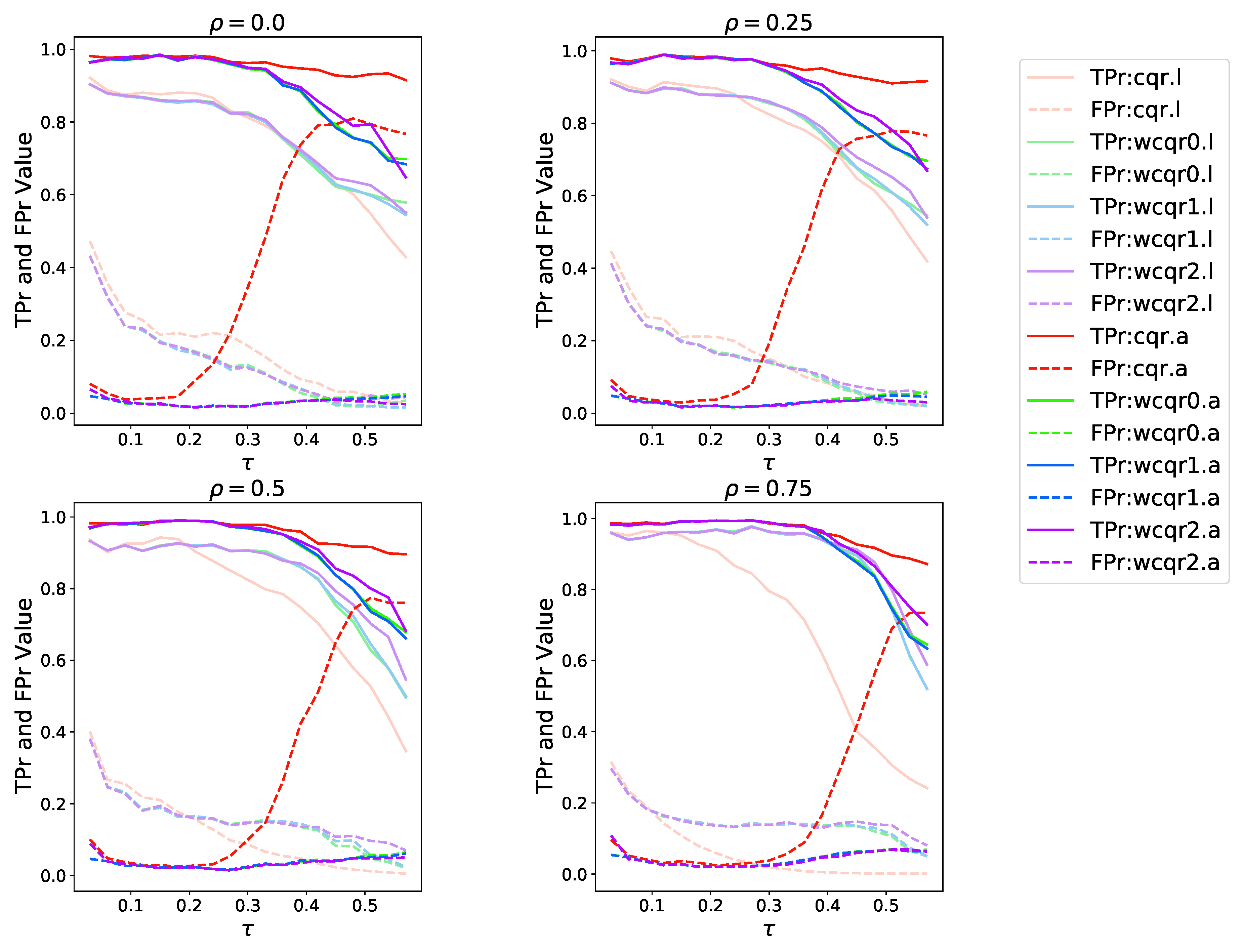
We use the following criteria to evaluate the performances: the ratio of number of relevant variables correctly selected to true number of relevant variables (TPr) defined as $\mathrm{TPr}=\frac{\#\left\{\right\{j:|{\widehat{\beta }}_j\left(\tau \right)|\ne 0\}\cap \{j:|{\beta }_{0j}\left(\tau \right)|\ne 0\}\}}{\#\{j:|{\beta }_{0j}\left(\tau \right)|\ne 0\}}$, the ratio of number of irrelevant variables incorrectly selected to true number of irrelevant variables (FPr) defined as $\mathrm{FPr}=\frac{\#\{\{j:{\widehat{\beta }}_j\left(\tau \right)\ne 0\}\cap \{j:|{\beta }_{0j}|=0\}\}}{\#\{j:|{\beta }_{0j}|=0\}}$, the absolute error $P_1={\sum }_{j=1}^p|\widehat{{\beta }_j}\left(\tau \right)-{\beta }_{0j}\left(\tau \right)|$, and the squared error $P_2={\sum }_{j=1}^p|{\widehat{\beta }}_j\left(\tau \right)-{\beta }_{0j}\left(\tau \right){\left)\right|}^2$. The closer TPr is to 1 and FPr is to 0, the better. Both TPr and FPr range from 0 to 1, thus we present them together in Figure 1 for comparison.

Figure 1. Case $n=200,s=30,p_0=0.8,p_1=0.6$. Comparison of TPr and FPr for four levels of $\rho$. In each subplot, the Y axis reports the TPr and FPr values at different $\tau$. The solid line is TPr and the dashed line is FPr. Four colors are used to represent the methods: red for wcqr, green for wcqr0, blue for wcqr1, and purple for wcqr2. Light colors represent the LASSO penalty and dark colors are the ALASSO penalty for all methods.

We compare our proposed weighted estimators with the estimated estimator of competing risks quantile regression model proposed in [8], denoted as wcqr and cqr, respectively, implying the weighting method or not. In simulation tables, we use cqr.l and cqr.a to represent cqr estimators with LASSO and ALASSO penalty, respectively. Similarly, our estimators, denoted as wcqri.l and wcqri.a, $i=0,1$ stands for administrative censoring where C is known and randomly right censoring cases where X is in place of C, respectively; wcqr2 uses a different weight:

$$\begin{array}{ccc}\hfill w_i\left(F_1\right)& =& \left\{\begin{array}{cc}1\hfill & {\delta }_i{ϵ}_i=1\hfill \\ \frac{\tau -{\widehat{F}}_1\left(C_i\right)}{1-{\widehat{F}}_1\left(C_i\right)-{\widehat{F}}_2\left(C_i\right)}\hfill & {\delta }_i=0,{\widehat{F}}_1\left(C_i\right)<\tau \hfill \\ 0\hfill & \mathrm{otherwise}.\hfill \end{array}\right.\hfill \end{array}$$

As the weight above involves the estimation of $F_2\left(t\right|Z)=P(T\le t,ϵ=2|Z)$, which probably is complicated in practical circumstances, we only use it for comparison in simulations. Here in wcqr2, we apply a similar estimating method of $F_1$ to $F_2$.

Alhough our theoretical results are not based on these two estimators of $w_i$, most simulation results show that wcqr0 and wcqr1 are considerably close, as the weight is only different at $\delta =1$, suggesting good estimates in large censoring rates. Research about massive competing risks data with enormous censored observations will appear in our future work.

Before the variable selection, we also conduct the simulation for unpenalized estimators. In this case, we use ${\gamma }_0=(1,-1.5,-0.5)$, $p_0=0.8,p_1=0.6$, and $\rho =0$. We repeat this 1000 times and compare the empirical bias (EmpBias) and average coverage probabilities based on 95% confidence intervals computed with empirical variance. The results are summarized in Table 1, where in lower quantiles, the cqr method shows extreme excellence, whereas in high quantiles, it displays some instability. For weighted methods, though inferior to cqr in lower quantiles, these methods still behave well in most simulations, especially wcqr1 and wcqr2. The average coverage probabilities display similar patterns; cqr behaves well until $\tau <0.4$. In relatively high quantiles such as $\tau =0.5$, wcqr2 behaves the best for most coefficients.

Table 1. Bias and empirical coverage; $n=300,\rho =0,p_0=0.8,p_1=0.6$.

$\mathit{\tau }$	Method	Bias				EmpCoverage
		${\mathbf{\beta }}_{\mathbf{1}}$	${\mathbf{\beta }}_{\mathbf{2}}$	${\mathbf{\beta }}_{\mathbf{3}}$	${\mathbf{\beta }}_{\mathbf{4}}$	${\mathbf{\beta }}_{\mathbf{1}}$	${\mathbf{\beta }}_{\mathbf{2}}$	${\mathbf{\beta }}_{\mathbf{3}}$	${\mathbf{\beta }}_{\mathbf{4}}$
0.1	cqr	−0.012	−0.003	0.003	0.003	0.952	0.953	0.953	0.958
	wcqr1	−0.027	−0.026	0.031	0.014	0.950	0.952	0.950	0.949
	wcqr2	−0.027	−0.032	0.036	0.018	0.948	0.952	0.946	0.950
0.2	cqr	0.000	−0.015	−0.007	0.008	0.946	0.950	0.943	0.952
	wcqr1	−0.024	−0.061	0.042	0.032	0.948	0.944	0.949	0.943
	wcqr2	−0.019	−0.081	0.055	0.040	0.949	0.940	0.952	0.940
0.3	cqr	−0.010	−0.023	0.008	0.014	0.947	0.949	0.956	0.953
	wcqr1	−0.042	−0.108	0.095	0.055	0.938	0.952	0.944	0.943
	wcqr2	−0.027	−0.131	0.104	0.065	0.939	0.949	0.934	0.941
0.4	cqr	0.219	−1.244	−0.069	0.316	0.999	0.999	0.999	0.999
	wcqr1	−0.065	−0.203	0.168	0.121	0.947	0.943	0.931	0.937
	wcqr2	0.007	−0.153	0.111	0.095	0.949	0.939	0.941	0.922
0.5	cqr	−5.878	−25.526	−12.526	10.139	0.975	0.957	0.967	0.953
	wcqr1	−0.313	−0.632	0.594	0.280	0.965	0.943	0.963	0.914
	wcqr2	0.144	0.034	0.041	−0.007	0.913	0.955	0.952	0.953

With moderate dimensions of covariates ($s=30$), Figure 1 presents the TPr and FPr values evaluated for $n=200$ and $\tau \in (0,0.6)$ and four $\rho$s for ${\Sigma }_1$, respectively. Generally speaking, we can observe that almost all selection performances appear to decline as $\tau$ increases, and with higher TPr and lower FPr, ALASSO penalized methods are overall superior to LASSO methods. Specifically, in quantiles lower than 0.4, with ALASSO penalty, cqr and wcqr both have good performances for identification of important variables, with TPr close to 1. Compared to the ALASSO method, LASSO methods have higher FPr values and tend to select much more irrelevant variables. In Figure 1, wcqr estimators display comparable performance with cqr estimators according to high TPr and low FPr at moderate $\tau \in (0,0.35)$. At higher quantiles, although a little bit inferior to cqr estimators in TPr, wcqr estimators have very low FPr values despite a rapid increase of FPr for cqr estimators, which means wcqr estimators have a strong ability to drop irrelevant variables as well as select correct variables even when cqr estimators almost fail in particularly high quantiles. We should state that in all simulations, wcqr estimators present quite stable performances in higher quantiles and higher dimensions. The decline of performance with increasing $\tau$ can be explained by a higher $\tau$ that is approaching the probability $P(ϵ=1|Z)$, which induces larger biases. In addition, it is notable that TPr has a very small decrease when $\rho$ increases except for cqr.l, which has a large decrease, since when the correlation of covariates increases, it is more difficult for identification. Even when $\rho =0.75$, the wcqr estimators with ALASSO behave quite well in simulations.

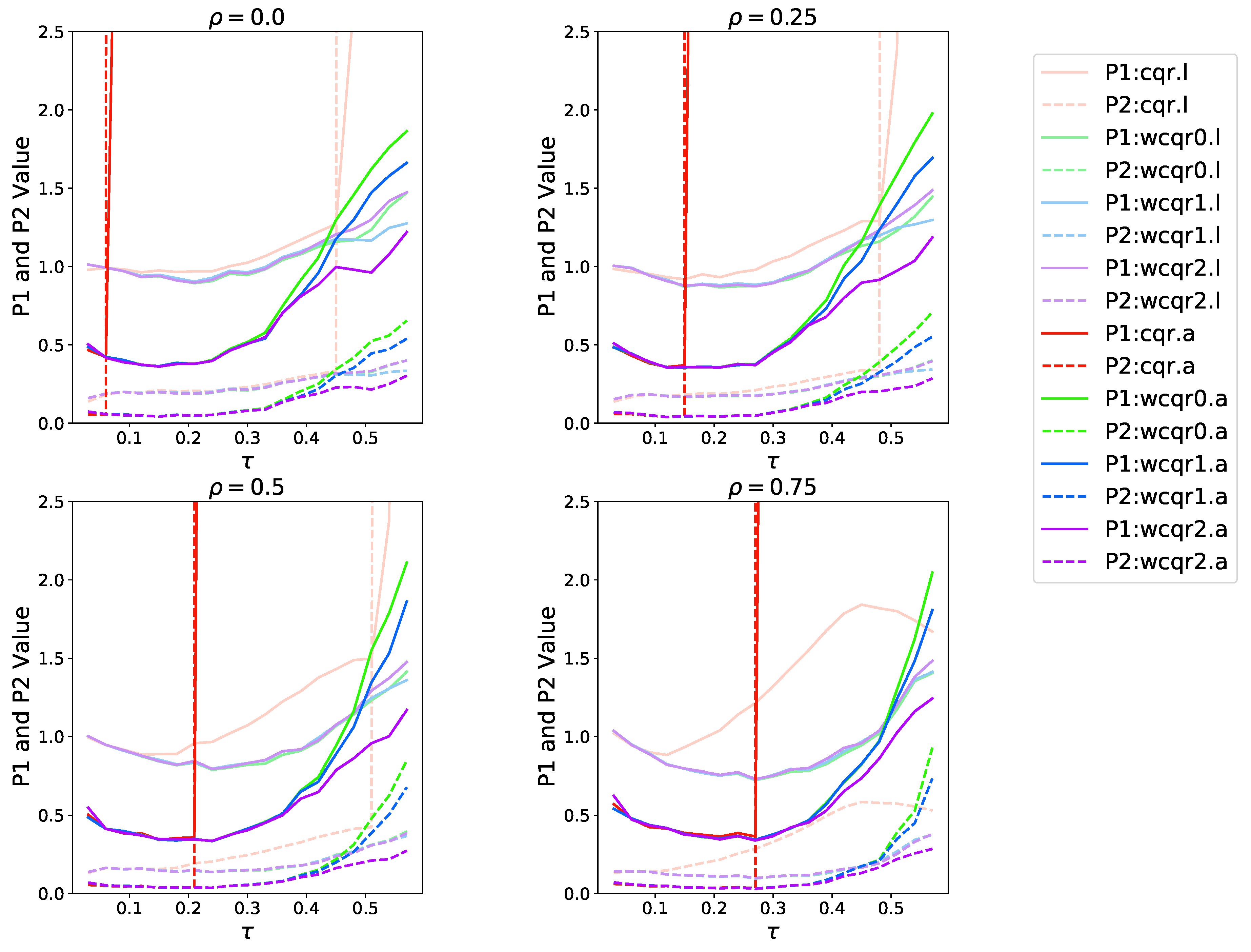
Figure 2 shows the P1 and P2 performances for the eight methods, and the two values for cqr estimators are too large to be displayed in the plot. In contrast, wcqr estimators stably indicate a decrease from 0.1 to about 0.27 and an increase from 0.3 to 0.6. It can be explained that in low quantiles, few ambiguous cases are used for estimation, which causes insufficient use of information; whereas in high quantiles, where more ambiguous observations are weighted, the accuracy of weights will affect the estimation performance. The improvement of estimation for $w_{0i}$ can be an investigation in the future.

Figure 2. Case $n=200,s=30,p_0=0.8,p_1=0.6$. Comparison of P1 and P2 for four levels of $\rho$. In each subplot, the Y axis reports the P1 and P2 values at different $\tau$. The solid line is P1 and the dashed line is P2. Four colors are used to represent the methods: red for cqr, green for wcqr0, blue for wcqr1, and purple for wcqr2. Light colors represent the LASSO penalty and dark colors are the ALASSO penalty for all methods.

We also present other simulation results in Figures S1–S11 in the supplementary material. Figures S1 and S2 show the TPr, FPr, P1, and P2 for $s=20$ and 50, respectively. We can observe that, in Figure S1, the TPr of wcqr estimators with ALASSO are above 0.9 except for very high quantiles, indicating stability with low FPr compared to cqr estimators; in Figure S2, the tendency remains but the selection performance is inferior, although TPr still stays higher than 0.8 at $\tau =0.4$. We also conduct the case when $s=100,n=100$, which means the number of predictors exceeds the sample size. In this case, cqr estimators fail due to singular design matrix as well as the ALASSO estimator. We discover, surprisingly, that our wcqr estimators still work and behave quite well, as illustrated in Figure S3. Numerical studies for $s=10$ and ${\gamma }_0=(-2,-2.5,0.5,0,\cdots ,0)$ are also discussed in the supplementary material, illustrated by Figures S4–S11. For the structure of the covariance matrix, we consider another kind of setup: ${\Sigma }_{2,ij}={\rho }^{|i-j|}$. We also consider a different choice for $p_0$ and $p_1$ as 0.6 and 0.45, respectively, in order to test the performance under a different probability of $P({ϵ}_i=1)$. In addition, we also simulate the heavy-tailed distributions $t\left(3\right)$ instead of Gaussian distribution for $P(T\le t|ϵ=1,Z)$. Figures S4–S7 show that the ALASSO penalty significantly decreases the FP for both estimators, which suggests the superiority of ALASSO. Our estimators behave fairly close to the cqr estimator in most cases. Although the TP of our estimators behave slightly worse, the FP shows a relatively better performance. Not only does wcqr shows smaller deviation about estimated coefficients, but it also shows great stability, especially for the ALASSO penalty, in the case of higher quantiles $\tau =0.5$. This shows the meaningful application of our estimators in high quantiles. Figure S8 represents the case of $n=400$, where the performances of all criteria are greatly improved.

Figure S9 shows the performance for ${\Sigma }_2$, which presents slightly better results than the case of ${\Sigma }_1$. Figure S10 is for a different pair of $(p_0,p_1)=(0.6,0.45)$, and our $\tau$s ranges from 0 to 0.4, and $\tau =0.3$ turns out to be the quantile of 3 nonzero coefficients, which fits our simulation results. Figure S11 simulates t(3) distribution in place of standard normal distribution, displaying that our estimators behave significantly well for heavy-tailed distributions.

To conclude, wcqr estimators behaves comparably with the cqr estimator, with slightly worse performance for TP but better for FP. Interestingly, for the higher correlations and higher quantiles and heavy-tailed distribution, the superior performance the wcqr estimators display show good potential applicability to more complex data and higher quantiles.

4.2. Real Data Analysis

In this subsection, we use the BMT dataset in [1] for practical application. As the simulation illustrates, wcqr estimators display more stability to the complexity of data and high quantiles than existing cqr estimators, which motivates us to conduct the data analysis with our methods.

In this dataset, a total of 177 patients received a stem cell transplant for acute leukemia. The failure event is relapse (REL, 56 patients), and death from causes related to the transplant (transplant related mortality, TRM, 75 patients) is the competing risk. Forty-six patients are censored, thus the censoring rate is 26%. Covariates that affect REL and TRM includes sex, disease (lymphoblastic or myeloblastic leukemia), phase at transplant (Relapse, CR1, CR2, CR3), source of stem cells (bone marrow and peripheral blood, coded as BM+PB, or peripheral blood, coded as PB), and age. The link function is assumed to be exponential.

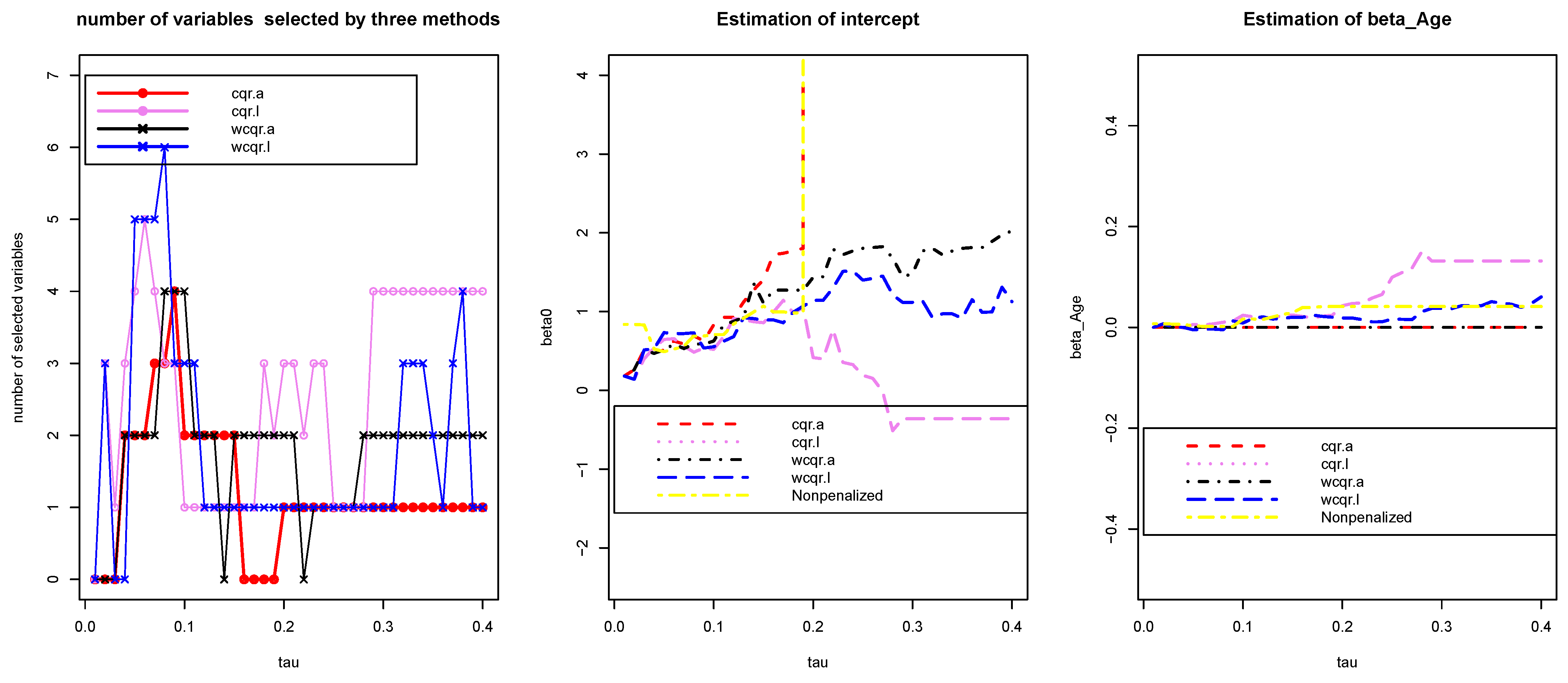
Figure 3, Figure 4 and Figure 5 report the numbers of selected variables as well as coefficient estimates by our weighted estimators compared with penalized quantile estimating equations proposed by [8] and the penalty-free methods with $\tau$ ranging from 0 to $0.4$.

Figure 3. Variable selection and estimation results for intercept and ${\beta }_{\mathrm{Age}}$. The Y axis reports the coefficient values at different $\tau$. Various colors of lines represent eight methods.

Figure 4. Estimation results for ${\beta }_{\mathrm{Sex}:\mathrm{F}}$, ${\beta }_{\mathrm{D}:\mathrm{AML}}$, and ${\beta }_{\mathrm{Phase}:\mathrm{CR}1}$.The Y axis reports the coefficient values at different $\tau$. Various colors of lines represent eight methods.

Figure 5. Estimation results for ${\beta }_{\mathrm{Phase}:\mathrm{CR}2}$, ${\beta }_{\mathrm{Phase}:\mathrm{CR}3}$ and ${\beta }_{\mathrm{Source}:\mathrm{PB}}$. The Y axis reports the coefficient values at different $\tau$. Various colors of lines represent eight methods.

From the figure we can see mainly our estimators select similar numbers of variables to cqr estimators at lower quantiles, but in higher quantiles, the wcqr estimators lie between the cqr-LASSO and cqr-ALASSO. For the intercept, in lower quantiles, five estimators appears conincident with one another, although cqr-ALASSO estimators tend to be unstable, whereas wcqr estimators shows stability here. For age, all estimators regard this variable as unimportant, except that the two LASSO estimators probably overestimate the importance. For sex:F, almost all estimators shrink the corresponding coefficients to zero. The ALASSO estimators tend to treat D:AML as an unimportant variable, except for quantiles around 0.1. For phase:CR1 and phase:CR2, all estimators tend to select them in lower quantiles, but wcqr tends to select phase:CR1 at higher quantiles larger than 0.21 but neglects phase:CR2 from 0.22 to 0.27. For phase:CR3, all the estimators show analogue performances but with slight shifts. For source:PB, the wcqr estimators perform more stably than cqr for all quantiles. The estimations for $F_1$ based on the five methods are placed in Figure 6.

Figure 6. Estimation of $F_1$. The Y axis reports the estimated values of $F_1\left(t\right)$ at different t. Various colors of lines represent eight methods.

To conclude, our wcqr estimators present stability and keep similar performances to the results of cqr estimators. More importantly, our weighted estimates provide a relatively general objective function for researchers to directly use R packages for application.

5. Conclusions

In this paper, we proposed a weighted method for competing risks quantile regression model to transform the estimating equation to a common weighted objective function and applied the LASSO and ALASSO penalization for variable selection. We established the consistency and asymptotic normality for penalty-free estimators as well as the consistency of variable selection. Monte Carlo simulations were conducted for several scenarios, presenting good variable selection performance and stability. Finally, a real dataset was utilized to illustrate the application of our methods, which is comparable with other methods.

References

- Scrucca, L.; Santucci, A.; Aversa, F. Regression modeling of competing risk using R: An in depth guide for clinicians. Bone Marrow Transpl. 2010, 45, 1388–1395. [Google Scholar] [CrossRef] [PubMed]
- Fine, J.P.; Gray, R.J. A proportional hazards model for the subdistribution of a competing risk. J. Am. Stat. Assoc. 1999, 94, 496–509. [Google Scholar] [CrossRef]
- Fu, Z.; Parikh, C.R.; Zhou, B.J. Penalized variable selection in competing risks regression. Lifetime Data Anal. 2017, 23, 353–376. [Google Scholar] [CrossRef] [PubMed]
- Koenker, R.W.; Bassett, G. Regression quantile. Econometrica 1978, 46, 33–50. [Google Scholar] [CrossRef]
- Peng, L.; Fine, J.P. Competing risks quantile regression. J. Am. Stat. Assoc. 2009, 104, 1440–1453. [Google Scholar] [CrossRef]
- Sun, Y.Q.; Wang, H.; Gilbert, P. Quantile regression for competing risks data with missing cause of failure. Stat. Sin. 2012, 22, 703–728. [Google Scholar] [CrossRef] [PubMed]
- Ahn, K.W.; Kim, S. Variable selection with group structure in competing risks quantile regression. Stat. Med. 2018, 37, 1577–1586. [Google Scholar] [CrossRef] [PubMed]
- Li, E.; Tian, M.; Tang, M. Variable selection in competing risks models based on quantile regression. Stat. Med. 2019, 38, 4670–4685. [Google Scholar] [CrossRef] [PubMed]
- Wang, H.J.; Wang, L. Locally weighted censored quantile regression. J. Am. Stat. Assoc. 2009, 104, 1117–1128. [Google Scholar] [CrossRef]
- Tibshirani, R. Regression shrinkage and selection via the lasso. J. R. Stat. Soc. B. 1996, 58, 267–288. [Google Scholar] [CrossRef]
- Zou, H. The adaptive lasso and its oracle properties. J. Am. Stat. Assoc. 2006, 101, 121–152. [Google Scholar] [CrossRef]
- Gray, R.J. A class of k-sample tests for comparing the cumulative incidence of a competing risk. Ann. Stat. 1988, 16, 1141–1154. [Google Scholar] [CrossRef]
- Koenker, R. Quantile Regression; Cambridge University Press: New York, NY, USA, 2005. [Google Scholar]
- Wang, H.J.; Zhou, J.; Li, Y. Variable selection for censored quantile regresion. Stat. Sin. 2013, 23, 145–167. [Google Scholar] [PubMed]
- Robins, J.M.; Rotnitzky, A. Recovery of information and adjustment for dependent censoring using surrogate markers. In AIDS Epidemiology Theorethodological Issues; Jewell, N., Dietz, K., Farewell, V., Eds.; Birkhäuser: Boston, MA, USA, 1992; pp. 24–33. [Google Scholar]
- Kaplan, E.L.; Meier, P. Nonparametric estimation from incomplete observations nonparametric estimation from incomplete observations. J. Am. Stat. Assoc. 1958, 53, 457–481. [Google Scholar] [CrossRef]
- Pepe, M.S. Inference for Events With Dependent Risks in Multiple Endpoint Studies. J. Am. Stat. Assoc. 1991, 86, 770–778. [Google Scholar] [CrossRef]
- Chen, X.; Linton, O.; Van Keilegom, I. Estimation of semiparametric models when the criterion function is not smooth. Econometrica 2003, 71, 1591–1608. [Google Scholar] [CrossRef]
- van der Vaart, A.W. Asymptotic Statistics; Cambridge University Press: Cambridge, UK, 1998. [Google Scholar]
- Jureckova, J. Asymptotic relations of m-estimates and r-estimates in linear regression. Ann. Statist. 1977, 5, 464–472. [Google Scholar] [CrossRef]
Disclaimer/Publisher’s Note: The statements, opinions and data contained in all publications are solely those of the individual author(s) and contributor(s) and not of MDPI and/or the editor(s). MDPI and/or the editor(s) disclaim responsibility for any injury to people or property resulting from any ideas, methods, instructions or products referred to in the content. |
© 2023 by the authors. Licensee MDPI, Basel, Switzerland. This article is an open access article distributed under the terms and conditions of the Creative Commons Attribution (CC BY) license (https://creativecommons.org/licenses/by/4.0/).