A Novel Model for Quantitative Risk Assessment under Claim-Size Data with Bimodal and Symmetric Data Modeling

Abstract

A novel flexible extension of the Chen distribution is defined and studied in this paper. Relevant statistical properties of the novel model are derived. For the actuarial risk analysis and evaluation, the maximum likelihood, weighted least squares, ordinary least squares, Cramer–von Mises, moments, and Anderson–Darling methods are utilized. For actuarial purposes, a comprehensive simulation study is presented using various combinations to evaluate the performance of the six methods in analyzing insurance risks. These six methods are used in evaluating actuarial risks using insurance claims data. Two applications on bimodal data are presented to highlight the flexibility and relevance of the new distribution. The new distribution is compared to several competing distributions. Actuarial risks are analyzed and evaluated using actuarial data, and the ability to disclose actuarial risks is compared by a comprehensive simulation study, through which actuarial disclosure models are compared using a wide range of well-known models.

1. Introduction

There are several justifications for creating a risk measurement system; such a technique is often used to compare and measure risk. Considering this, we must make sure that any risk measuring system generates coherent findings or at the very least can spot situations where it might not be. The two independent random variables (RVs) employed in each property claim procedure are the claim-count RV and the claim-size RV. The aggregate-loss RV (ALRV), which is produced by combining the first two fundamental claim RVs, represents the total claim amount produced by the underlying claim process. Following Chen [1], a novel flexible extension of the Chen distribution called the generalized Rayleigh Chen (GRC) is defined and studied in this work.

The new risk-density function is used in risk exposure analysis, risk assessment, and risk analysis under some actuarial indicators. Several actuaries employ a broad variety of parametric families of continuous distributions to model the size of property and casualty insurance claim amounts. An examination of the actuarial literature for insurance claims data finds that it is mostly right skewed (see Cooray and Ananda [2], Shrahili et al. [3] and Mohamed et al. [4]). This work analyses and models some data sets including a new actuarial data set of negatively skewed insurance claims. Additionally, the risk exposure is an actuarial estimation of the potential loss that could develop in the future because of a specific action or occurrence. Risks are often ranked according to their likelihood of happening in the future multiplied by the potential loss if they did as part of an assessment of the business’s risk exposure. By assessing the likelihood of expected losses in the future, insurance and reinsurance companies may distinguish between little and major losses. Speculative risks frequently lead to losses, including breaking rules, losing brand value, having security flaws, and having liability problems. Generally, the risk exposure (${\nabla }_{RE}$) can be calculated from:

$${\nabla }_{RE}\left(x\right)=T\left(x\right)\times \mathrm{Pr}\left(x\right),$$

where $T\left(x\right)$ is the total loss of the risk occurrence, and $\mathrm{Pr}\left(x\right)$ refers to the probability of the risk occurring. On the other hand, extensive research has been put into employing time series analysis, regression modelling, or continuous distributions to analyze historical insurance data. Actuaries have recently used continuous distributions, especially ones with long tails, to reflect actual insurance data (see, for example, Mohamed et al. [4] and Shrahili et al. [3]). Using continuous heavy-tailed probability distributions, real data have been modeled in a number of real-world applications, including engineering, risk management, dependability, and the actuarial sciences. Due to its monotonically decreasing density form, the Pareto model does not offer a good fit for many actuarial applications when the frequency distributions are hump-shaped. The lognormal is frequently used to model these data sets in these circumstances. It is obvious that neither the lognormal nor the Pareto can account for left-skewed payment data. To address this flaw in the outdated conventional models, we provide the GRC distribution for the left-skewed actuarial claims.

Distributions based on probabilities can provide an accurate depiction of the risk exposure and have been recently used for this actuarial purpose (see Shrahili et al. [3] and Mohamed et al. [4]). The levels of exposure are functions frequently referred to as major risk indicators (RIs) (Klugman et al. [5] ). Such RIs provide risk managers and actuaries with information on the level of risk that the firm is exposed to. There are a variety of RIs that can be taken into consideration and researched, including tailed-value-at-risk (TVAR) (also known as the conditional tail expectation (CTE)). We also study how the mean excess loss (MEL) function may be used to reduce actuarial and economic risks, (see Wirch [6], value-at-risk (VAR), (see Wirch [6], Tasche [7], and Acerbi [8] ), conditional-VAR (CVAR), and tail-variance (TV) (see Furman and Landsman [9] and Landsman [10]).

The probability distribution of massive losses in particular is quantized by the VAR. Actuaries and risk managers usually concentrate on calculating the probability of a bad outcome. The probability of a negative outcome can be represented by the VAR indicator at a given probability/confidence level. Calculating the amount of money required to plan for these potentially devastating circumstances is typically performed using the VAR indicator.

The capacity of the insurance firm to handle such occurrences is of importance to actuaries, regulators, investors, and rating agencies. The GRC model, which is a novel model, takes into account certain RIs, including VAR, TMV, TVAR, and TV, for the left-skewed actuarial claims data (see Artzner [11]).

2. The New Model

Due to Chen [1], the cumulative distribution function (CDF) of the Chen (C) model is given by

$$W_{\theta ,\beta }\left(x\right)=1-\mathit{exp}\left[\beta -\beta \mathit{exp}\left(x^{\theta }\right)\right]\}{|}_{x>0},$$

(1)

where $\theta ,\beta >0$ control the shape of the C distribution. For $\beta =1$, the C model reduces to another one-parameter C model. The hazard rate function (HRF) of the C model just has a U-shape (decreasing–constant–increasing) for al $\theta <1$ and has “monotonically increasing HRF “when $\theta \ge 1$. The CDF of the generalized Rayleigh (GR-G) family (see Yousof et al. [12] and Cordeiro et al. [13]) is defined as

$$F_{\alpha ,\underset{\_}{\xi }}\left(x\right)={\left\{1-\mathit{exp}\left[-{\Pi }_{\underset{\_}{\xi }}^2\left(x\right)\right]\right\}}^{\alpha }{|}_{x\in R},$$

(2)

where $\alpha >0$ controls the shape of the GR-G family of distributions, ${\Pi }_{\underset{\_}{\xi }}\left(x\right)=\frac{W_{\underset{\_}{\xi }}\left(x\right)}{{\overline{W}}_{\underset{\_}{\xi }}\left(x\right)}$; $W_{\underset{\_}{\xi }}\left(x\right)$ refers to the CDF of the selected baseline model with baseline parameter vector $\underset{\_}{\xi };$ and ${\overline{W}}_{\underset{\_}{\xi }}\left(x\right)=1-W_{\underset{\_}{\xi }}\left(x\right)$ refers to the survival function (SF) (SF) of the baseline model with baseline parameter vector $\underset{\_}{\xi }$. Inserting Equation (1) into Equation (2), the CDF of the GRC distribution can be expressed as

$$F_{\underset{\_}{V}}\left(x\right)={\left\{1-\mathit{exp}\left[-{\Pi }_{\theta ,\beta }^2\left(x\right)\right]\right\}}^{\alpha }{|}_{x,\alpha ,\theta >0},$$

(3)

where ${\Pi }_{\theta ,\beta }^{}\left(x\right)=\frac{1-\mathit{exp}\left[\beta -\beta \mathit{exp}\left(x^{\theta }\right)\right]}{\mathit{exp}\left[\beta -\beta \mathit{exp}\left(x^{\theta }\right)\right]}$, $\underset{\_}{V}=\left(\alpha ,\theta ,\beta \right)$. The probability density function (PDF) corresponding to (3) can then be derived as

$$f_{\underset{\_}{V}}\left(x\right)=2\alpha \theta \beta x^{\theta -1}\frac{{\overline{C}}_{\theta ,\beta }\left(x\right)\mathit{exp}\left(x^{\theta }\right)}{C_{\theta ,\beta }^2\left(x\right)\mathit{exp}\left[{\Pi }_{\theta ,\beta }^2\left(x\right)\right]}{\left\{1-\mathit{exp}\left[-{\Pi }_{\theta ,\beta }^2\left(x\right)\right]\right\}}^{\alpha -1}{|}_{x,\alpha ,\theta >0},$$

(4)

where ${\overline{C}}_{\theta }\left(x\right)=1-C_{\theta }\left(x\right)$ and $C_{\theta ,\beta }\left(x\right)=\mathit{exp}\left[\beta -\beta \mathit{exp}\left(x^{\theta }\right)\right].$ The following quantile function can be used for simulating the GRC model:

$$X_{\upsilon }={\left(\mathit{log}\left[1-\mathit{log}\left(1-{\left\{1+{\left[-\frac{1}{\beta }\mathit{log}\left(1-u^{\frac{1}{\alpha }}\right)\right]}^{-1/2}\right\}}^{-1}\right)\right]\right)}^{\frac{1}{\theta }}, 0<u<1.$$

(5)

Figure 1 depicts the extensive flexibility of the new GRC PDF, which can be used to explore the new GRC PDF’s adaptability. A few PDF graphs for the GRC model are shown in Figure 1. Some HRF plots for the GRC model are shown in Figure 2.

Figure 1. Some PDF plots.

Figure 2. Some HRF plots.

We are motivated to define and study the GRC for the following reasons:

(1)

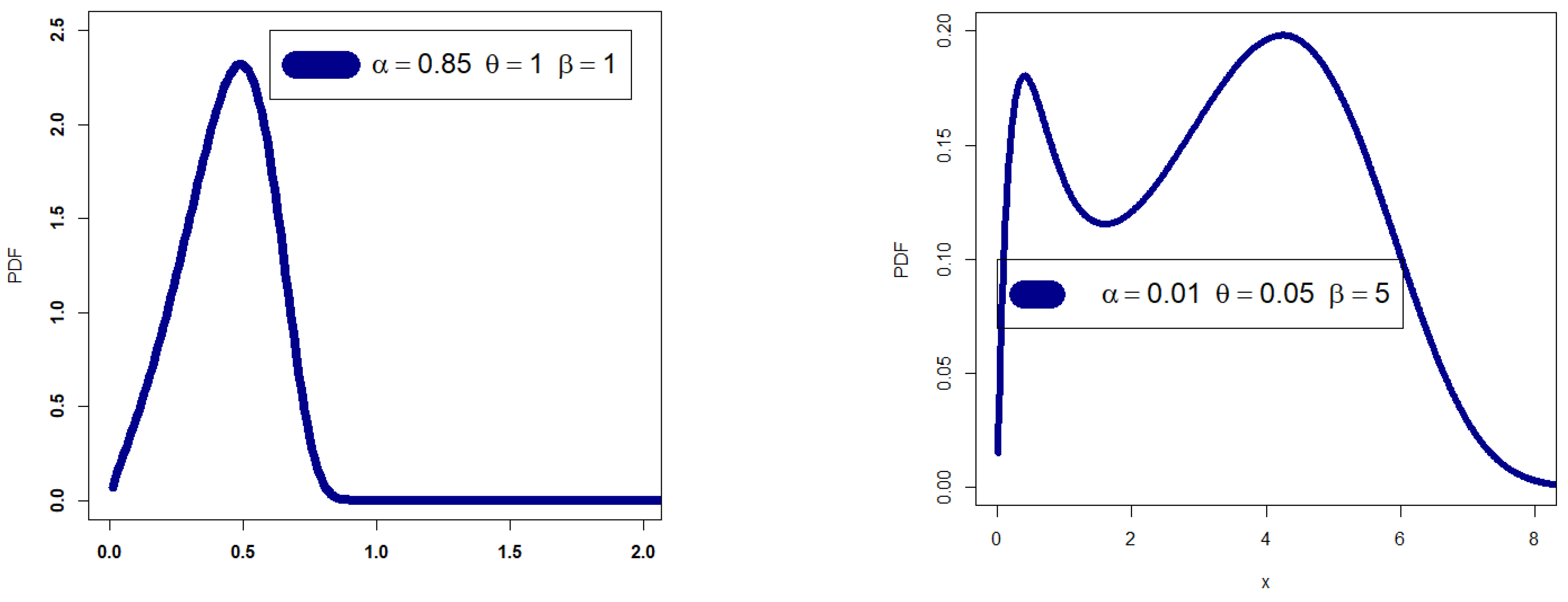
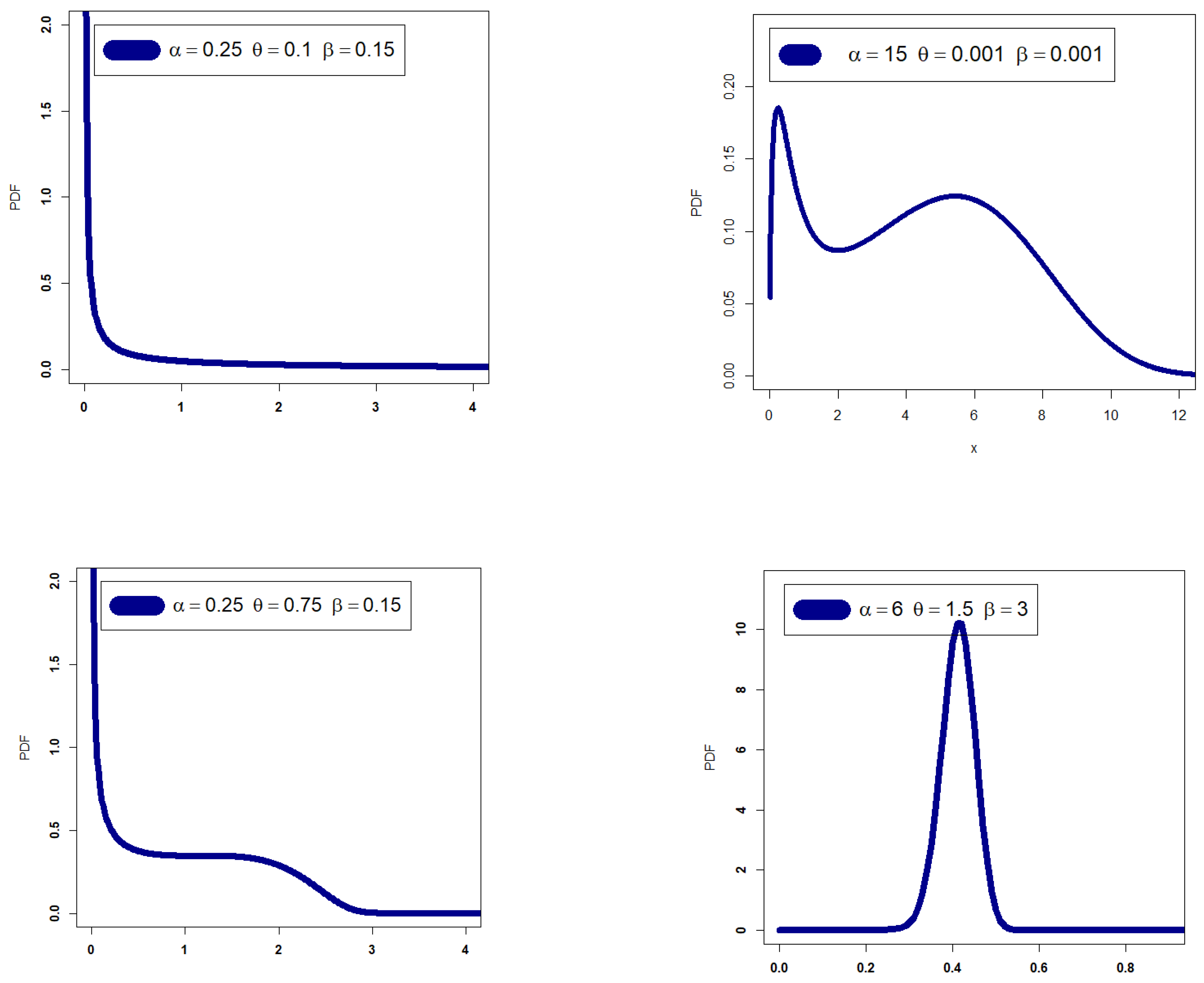
The new PDF in (4) can be “symmetric density”, “unimodal with right skewed shape”, “bimodal with right skewed shape”, and “left skewed density with no peaks” (see Figure 1).

(2)

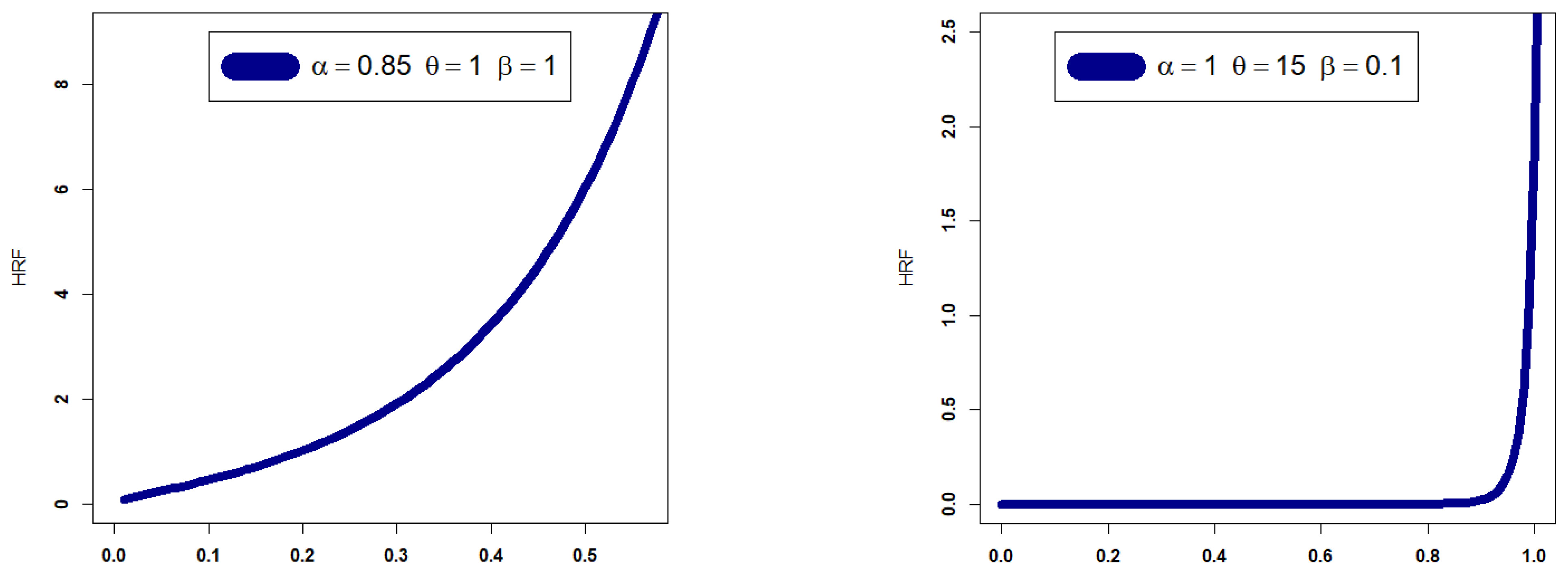
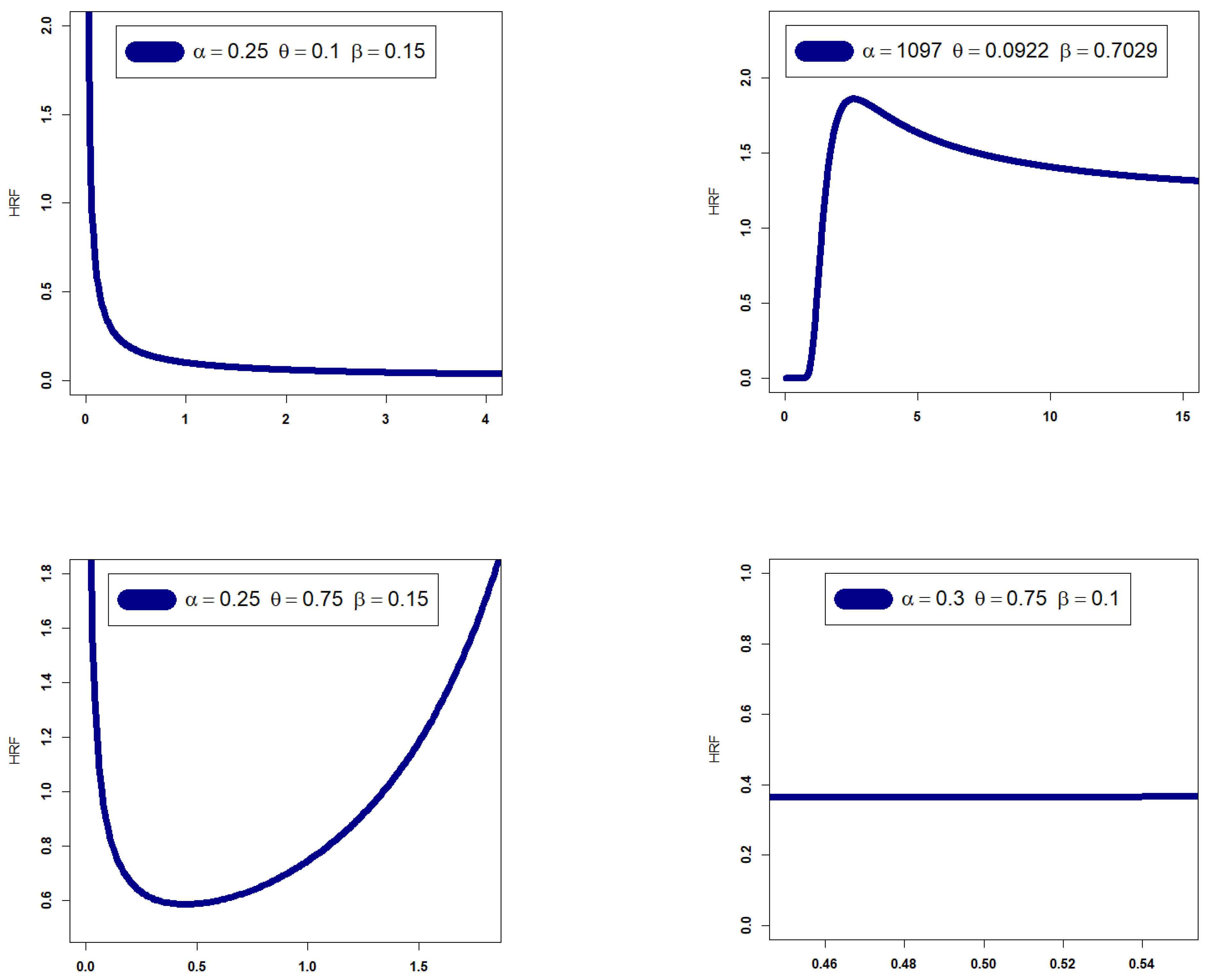
The HRF of the GRC model can be “monotonically increasing”, “J-HRF” and “upside down”, “decreasing–constant–increasing (bathtub)”, “monotonically decreasing”, and “constant-HRF “ (see Figure 2).

(3)

The GRC model may be selected as the optimum probabilistic model for reliability analysis, particularly when modelling the right heavy tail bimodal asymmetric and left heavy tail bimodal asymmetric real data.

3. Properties

3.1. Linear Representation

Using various algebraic techniques, such as the power series, the binomial expansion, and the extended binomial expansion, we summarize and simplify the PDF and the CDF of the GRC model in this section. We may readily obtain several of the GRC model’s associated mathematical and statistical features by simplifying the PDF and CDF. This section’s general goal is to express the PDF and CDF of the GRC model in terms of the exponentiated Chen (Ex-C) model. After that, it is possible to directly deduce the relevant mathematical and statistical characteristics of the exponentiated baseline model from those of the GRC model. Following Yousof et al. [12], the GRC density can then be expressed as

$$f_{\underset{\_}{V}}\left(x\right)=\stackrel{+\infty }{{\displaystyle \sum _{𝓀,𝒾=0}}}{\mathit{\nabla }}_{𝓀,𝒾}{h}_{\varpi ,\theta ,\beta }\left(x\right){|}_{\varpi =2𝓀+𝒾+2},$$

(6)

where

$$h_{\varpi ,\theta ,\beta }\left(x\right)=\varpi w_{\theta ,\beta }\left(x\right){\left[W_{\theta ,\beta }\left(x\right)\right]}^{\varpi -1},$$

(7)

is the Ex-C pdf with power parameter $\varpi$, $w_{\theta ,\beta }\left(x\right)=d{W}_{\theta ,\beta }\left(x\right)/dx$ and

$${\mathit{\nabla }}_{𝓀,𝒾}=\frac{2\alpha {\left(-1\right)}^{𝓀}\Gamma \left(\alpha \right)\Gamma \left(\varpi +1\right)}{\varpi 𝒾!𝓀!\Gamma \left(2𝓀+3\right)}\stackrel{+\infty }{{\displaystyle \sum _{𝒿=0}}}{\left(-1\right)}^{𝒿}\frac{{\left(𝒿+1\right)}^{𝓀}}{\Gamma \left(\alpha -𝒿\right)𝒿!}.$$

This formula can be derived directly from (6) as

$$F_{\underset{\_}{V}}\left(x\right)=\stackrel{+\infty }{{\displaystyle \sum _{𝓀,𝒾=0}}}{\mathit{\nabla }}_{𝓀,𝒾}{H}_{\varpi ,\theta ,\beta }\left(x\right){|}_{\varpi =2𝓀+𝒾+2},$$

(8)

where $h_{\varpi ,\theta ,\beta }\left(x\right)=d{H}_{\varpi ,\theta ,\beta }\left(x\right)/dx$. Two theorems related to the Ex-C model are presented in Dey et al. [14]. These two theorems are used in this paper, especially in actuarial indicators calculations. Using Equation (6) and the theorems of Dey et al. [14], one can derive many related properties for the new model. Equation (6) is the main result of this subsection and without deriving it, we will face many difficulties in deriving the properties of the new model.

3.2. Moments

Based on Theorem 1 of Dey et al. [14], the $𝓃\mathrm{th}$ ordinary moment of the GRC model can then be expressed as

$${\mu }_{𝓃,X}^{\prime }=E\left[X^{𝓃}\right]=\varpi \theta \stackrel{+\infty }{{\displaystyle \sum _{𝓀,𝒾,{\ell }_1,{\ell }_2=0}}}{\mathit{\nabla }}_{𝓀,𝒾}{\varpi }_{{\ell }_1}\left(\frac{𝓃}{\theta }\right){\varpi }_{{\ell }_2}\left(\frac{𝓃}{\theta }+{\ell }_1\right)\frac{{\left(-1\right)}^{\frac{2𝓃}{\theta }+{\ell }_1}}{{\beta }^{\frac{2𝓃}{\theta }+{\ell }_1}\left[\theta \left(\varpi +{\ell }_1+{\ell }_2\right)+𝓃\right]}$$

(9)

3.3. The Conditional Moments

The conditional moments $E\left(X^{𝓃}|X⟩x\right)$ can be expressed as

$$E\left(X^{𝓃}|X⟩x\right)=\varpi \theta \stackrel{+\infty }{{\displaystyle \sum _{𝓀,𝒾,{\ell }_1,{\ell }_2=0}}}\frac{{\mathit{\nabla }}_{𝓀,𝒾}{\varpi }_{{\ell }_1}\left(\frac{𝓃}{\theta }\right){\varpi }_{{\ell }_2}\left(\frac{𝓃}{\theta }+{\ell }_1\right){\left(-1\right)}^{\frac{2𝓃}{\theta }+{\ell }_1}{C}_{\theta ,\beta }\left(x\right)}{{\beta }^{\frac{2𝓃}{\theta }+{\ell }_1}\left[\theta \left(\varpi +{\ell }_1+{\ell }_2\right)+𝓃\right]\left\{1-{\left[1-C_{\theta ,\beta }\left(x\right)\right]}^{\varpi }\right\}}.$$

(10)

3.4. Rényi Entropy

The Rényi entropy is a measure of entropy, a concept in information theory, which is widely used in various fields, including actuarial risk analysis. In actuarial risk analysis, entropy measures are used to quantify the uncertainty or randomness associated with a set of data or events. The Rényi entropy is defined as a generalization of the Shannon entropy and can be used to capture the distributional properties of a random variable more effectively in certain cases. For instance, the Rényi entropy provides a more robust measure of entropy for distributions that are heavy tailed, have high kurtosis, or have other non-standard distributional properties.

In actuarial risk analysis, the Rényi entropy is particularly useful in the modeling of extreme events, such as catastrophic losses. For example, it can be used to quantify the risk associated with natural disasters, pandemics, or other extreme events that may have a significant impact on the insurance industry. The Rényi entropy can also be used to evaluate the uncertainty associated with the future development of the insured population or the underlying economic conditions, which can impact the performance of the insurance business. Generally, the Rényi entropy is a useful tool in actuarial risk analysis as it provides a more comprehensive measure of uncertainty and can be used to evaluate various types of risks. The Rényi entropy of the RV $X$ is defined by

$$I_{\delta }\left(X\right)=\frac{1}{\left(1-\delta \right)}\mathit{log}\left(\underset{-\infty }{\overset{+\infty }{{\displaystyle \int }}}f{\left(x\right)}^{\delta }dx\right){|}_{\delta >0\mathrm{and}\delta \ne 1}.$$

Using (4), we have

$$f_{\underset{\_}{V}}{\left(x\right)}^{\delta }={\displaystyle \sum }_{𝓀,𝒾=0}^{+\infty }{\tau }_{𝓀,𝒾}{x}^{\theta \delta -\delta }\mathit{exp}\left(\delta x^{\theta }\right)\mathit{exp}\left\{\delta \left[\beta -\beta \mathit{exp}\left(x^{\theta }\right)\right]\right\}{\left\{1-\mathit{exp}\left[\beta -\beta exp\left(x^{\theta }\right)\right]\right\}}^{2𝓀+𝒾+\delta },$$

where

$${\tau }_{𝓀,𝒾}={\left(2\alpha \theta \beta \right)}^{\delta }\stackrel{+\infty }{{\displaystyle \sum _{𝒿=0}}}\frac{{\left(-1\right)}^{𝒿+𝓀}{\left(\delta +𝒿\right)}^{𝓀}\Gamma \left(\left[\alpha -1\right]\delta +1\right)\Gamma \left(2𝓀+3\delta +𝒾\right)}{𝒿!𝓀!𝒾!\Gamma \left(2𝓀+3\delta \right)\Gamma \left(\left[\alpha -1\right]\delta -𝒿+1\right)}.$$

Then,

$$I_{\delta }\left(X\right)=\frac{1}{\left(1-\delta \right)}\mathit{log}\left[\stackrel{+\infty }{{\displaystyle \sum _{𝓀,𝒾=0}}}{\tau }_{𝓀,𝒾}{\displaystyle \underset{0}{\overset{+\infty }{\int }}}\left(\begin{array}{c}{x}^{\theta \delta -\delta }\mathit{exp}\left(\delta x^{\theta }\right)\mathit{exp}\left\{\delta \left[\beta -\beta exp\left(x^{\theta }\right)\right]\right\}\\ \times {\left\{1-\mathit{exp}\left[\beta -\beta \mathit{exp}\left(x^{\theta }\right)\right]\right\}}^{2𝓀+𝒾+\left(2-1\right)\delta }\end{array}\right)dx\right].$$

4. Actuarial Risk Indictors

4.1. VAR Indicator

Any insurance company will inevitably experience risk exposure. Actuaries developed a range of risk indicators as a result for statistically estimating risk exposure. VAR is an effort to calculate the most likely maximum amount of capital that might be lost over a predetermined amount of time. The maximum loss, which may be infinite or at least equal to the portfolio’s value, is not particularly instructive. Portfolios with the same maximum loss may differ greatly in their risk profiles. VAR therefore typically depends on the loss random variable’s probability distribution. The combined distribution of the risk variables impacting the portfolio determines how losses are distributed. There is a wealth of research on modelling risk factors and portfolio loss distributions that depend on the combined distribution of risk factors. Then, for GRC distributions, we can simply write

$$\stackrel{}{\mathrm{Pr}}\left(X>\sqrt[\theta ]{\mathit{log}\left[1-\mathit{log}\left(1-{\left\{1+\sqrt[2]{{\left[-\frac{1}{\beta }\mathit{log}\left(1-\sqrt[\alpha ]{q}\right)\right]}^{-1}}\right\}}^{-1}\right)\right]}\right)=\{\begin{array}{l}1\%{|}_{q=99\%}\hspace{1em}\\ 5\%{|}_{q=95\%}\hspace{1em}\\ ⋮\hspace{1em}\end{array}.$$

(11)

4.2. TVAR Risk Indicator

Let X denote a LRV. Then, the TVAR$q\left(X\right)$ at the $100 q\%$ confidence level is the expected loss given that the loss exceeds the $100 q\%$ of the distribution of $X$. Then, the TVAR($X$) can be expressed as

$$\epsilon \left(X\right)=E\left(X\right|X>𝜋\left(q\right))=\frac{1}{1-q}{\displaystyle \underset{𝜋\left(q\right)}{\overset{+\infty }{\int }}}x{f}_{\underset{\_}{V}}(x)dx.$$

(12)

Then, depending on Theorem 2 of Dey et al. [14], we have

$$\epsilon \left(X\right)=\frac{\varpi \theta }{1-q}\stackrel{+\infty }{{\displaystyle \sum _{𝓀,𝒾,{\ell }_1,{\ell }_2=0}}}{K}_{{\ell }_1,{\ell }_2}^{\left[1,\theta \right]}\frac{{\mathit{\nabla }}_{x,x}{\varpi }_{{\ell }_1}\left(\frac{1}{\theta }\right)C_{\theta }\left(x\right)}{K_{\varpi ,{\ell }_1,{\ell }_2}^{\left[1,\theta ,\beta \right]}\left\{1-{\left[1-C_{\theta }\left(x\right)\right]}^{\varpi }\right\}},$$

(13)

where $K_{{\ell }_1,{\ell }_2}^{\left[1,\theta \right]}={\varpi }_{{\ell }_2}\left(\frac{1}{\theta }+{\ell }_1\right){\left(-1\right)}^{\frac{2}{\theta }+{\ell }_1}$, $K_{\varpi ,{\ell }_1,{\ell }_2}^{\left[1,\theta ,\beta \right]}={\beta }^{\frac{2}{\theta }+{\ell }_1}\left[\theta \left(\varpi +{\ell }_1+{\ell }_2\right)+1\right],$ and ${\varpi }_{{\ell }_1}\left(\frac{1}{\theta }\right)$ is the coefficient of ${\left[\mathit{log}\left(1-t\right)\right]}^{\frac{2}{\theta }+{\ell }_1}$ in the expansion of ${\left\{{\sum }_{m_1=1}^{+\infty }\frac{1}{m_1}\left[log\right(1-t\left)\right]\right\}}^{\frac{1}{\theta }}$ and ${\varpi }_{{\ell }_2}\left(\frac{1}{\theta }+{\ell }_1\right)$ is the coefficient of $t^{{\ell }_1+{\ell }_2+\frac{1}{\theta }}$ in the expansion of ${\left({\sum }_{m_2=1}^{+\infty }\frac{t^{m_2}}{m_2}\right)}^{\frac{1}{\theta }+{\ell }_1}$. Thus, TVAR$\left(X\right)$ can be considered as the average of all VAR values above the confidence level $\ell$. This means that the TVAR$\left(X\right)$ indicator provides us more information about the tail of the GRC distribution. Finally, TVAR can also be expressed as

$$e\left(X\right)=\mathrm{TVAR}\left(X\right)-\mathrm{VAR}\left(X\right),$$

where $e\left(X\right)$ is the mean excess loss (MEL) function evaluated at the $100 q\mathrm{th}$ quantile.

4.3. TV Risk Indicator

Let $X$ denote an LRV. The TV risk indicator (TV ($X$)) can be expressed as

$$\mathrm{TV}\left(X\right)=E\left(X^2\right|X>𝜋(\ell ))-{\left[\mathrm{TVAR}\left(X\right)\right]}^2.$$

Then, depending on Theorem 2 of Dey et al. [14] and (15), we have

$$\mathrm{TV}\left(X\right)=\frac{\varpi \theta }{1-q}\stackrel{+\infty }{{\displaystyle \sum _{𝓀,𝒾,{\ell }_1,{\ell }_2=0}}}{K}_{{\ell }_1,{\ell }_2}^{\left[2,\theta \right]}\frac{{\mathit{\nabla }}_{𝓀,𝒾}{\varpi }_{{\ell }_1}\left(\frac{2}{\theta }\right)C_{\theta ,\beta }\left(x\right)}{K_{\varpi ,{\ell }_1,{\ell }_2}^{\left[2,\theta ,\beta \right]}\left\{1-{\left[1-C_{\theta ,\beta }\left(x\right)\right]}^{\varpi }\right\}}-{[\mathrm{TVAR}\left(X\right)]}^2.$$

(14)

where $K_{{\ell }_1,{\ell }_2}^{\left[2,\theta \right]}={\varpi }_{{\ell }_2}\left(\frac{2}{\theta }+{\ell }_1\right){\left(-1\right)}^{\frac{4}{\theta }+{\ell }_1}$, $K_{\varpi ,{\ell }_1,{\ell }_2}^{\left[2,\theta ,\beta \right]}={\beta }^{\frac{4}{\theta }+{\ell }_1}\left[\theta \left(\varpi +{\ell }_1+{\ell }_2\right)+2\right],$ and TVAR$\left(X\right)$ is given in (13).

4.4. TMV Risk Indicator

Let $X$ denote a loss LRV. The TMV risk indicator (TMV ($X$)) can then be expressed as

$$\mathrm{TMV}\left(X;\pi \right){|}_{0<\pi <1}=\mathrm{TVAR}\left(X;\pi \right)+\pi \mathrm{TV}\left(X;\pi \right).$$

(15)

Then, for any LRV, $\mathrm{TMV}\left(X;\pi \right)>$ $\mathrm{TV}\left(X;\pi \right)$, $\mathrm{TMV}\left(X;\pi \right)>$ $\mathrm{TVAR}\left(X;\pi \right)$, for $\pi =0,$ the $\mathrm{TMV}\left(X;\pi \right)=\mathrm{TVAR}\left(X;\pi \right),$ and for $\pi =1,$ the $\mathrm{TMV}\left(X;\pi \right)=\mathrm{TVAR}\left(X;\pi \right)+\mathrm{TV}\left(X;\pi \right)$.

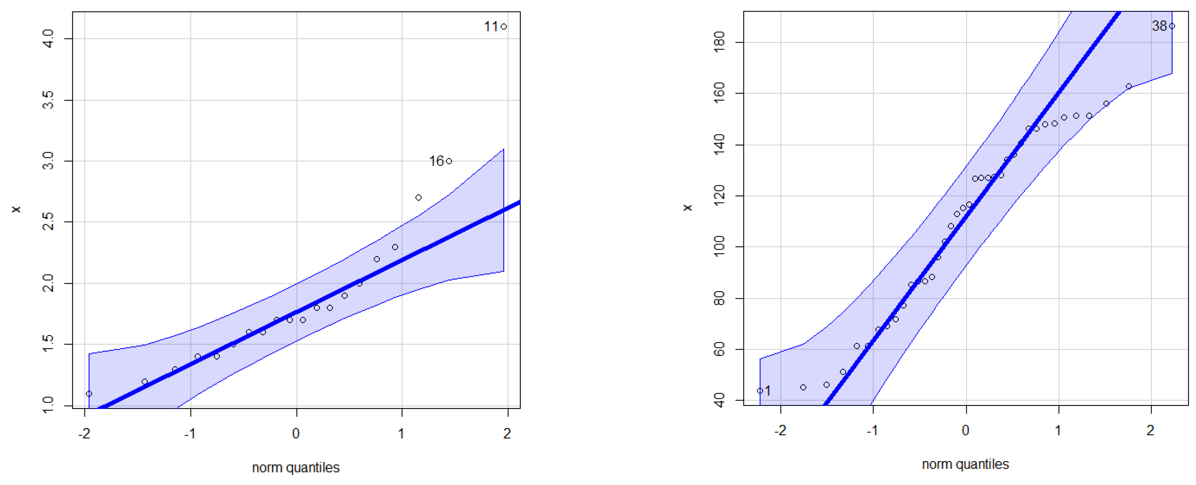
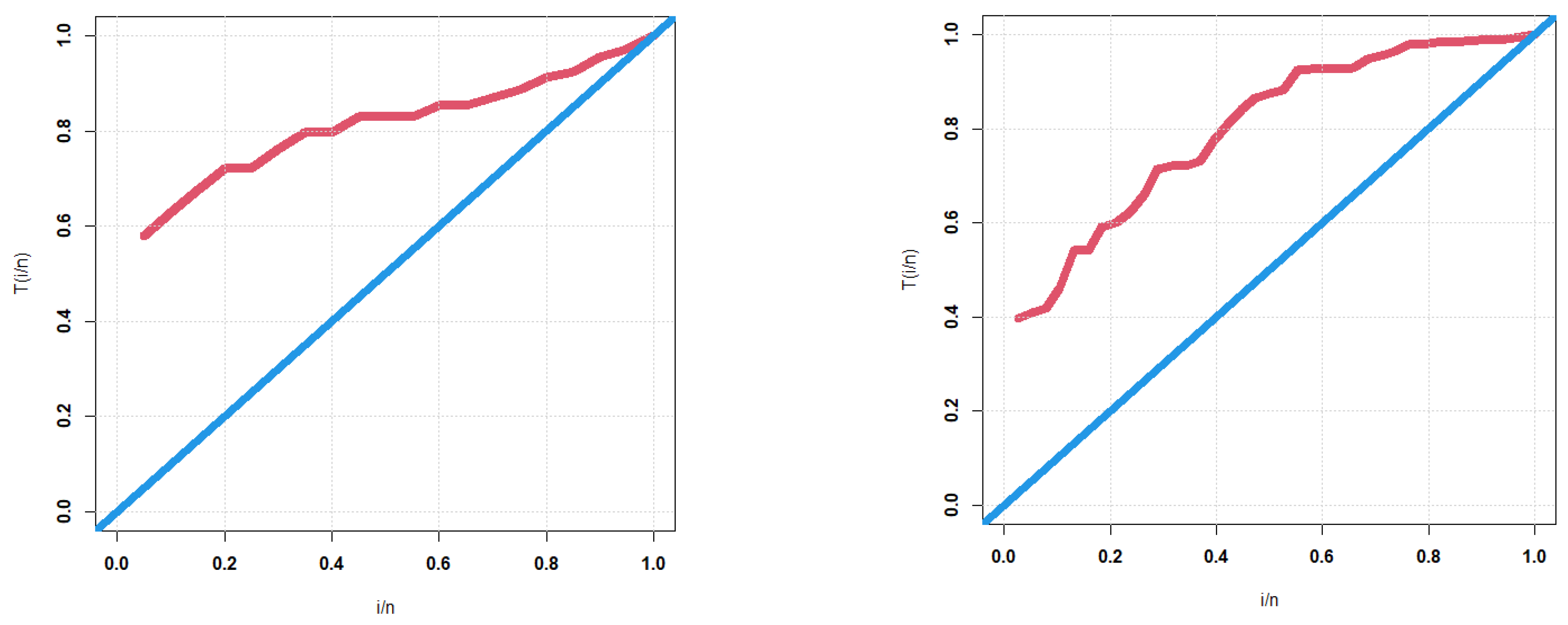
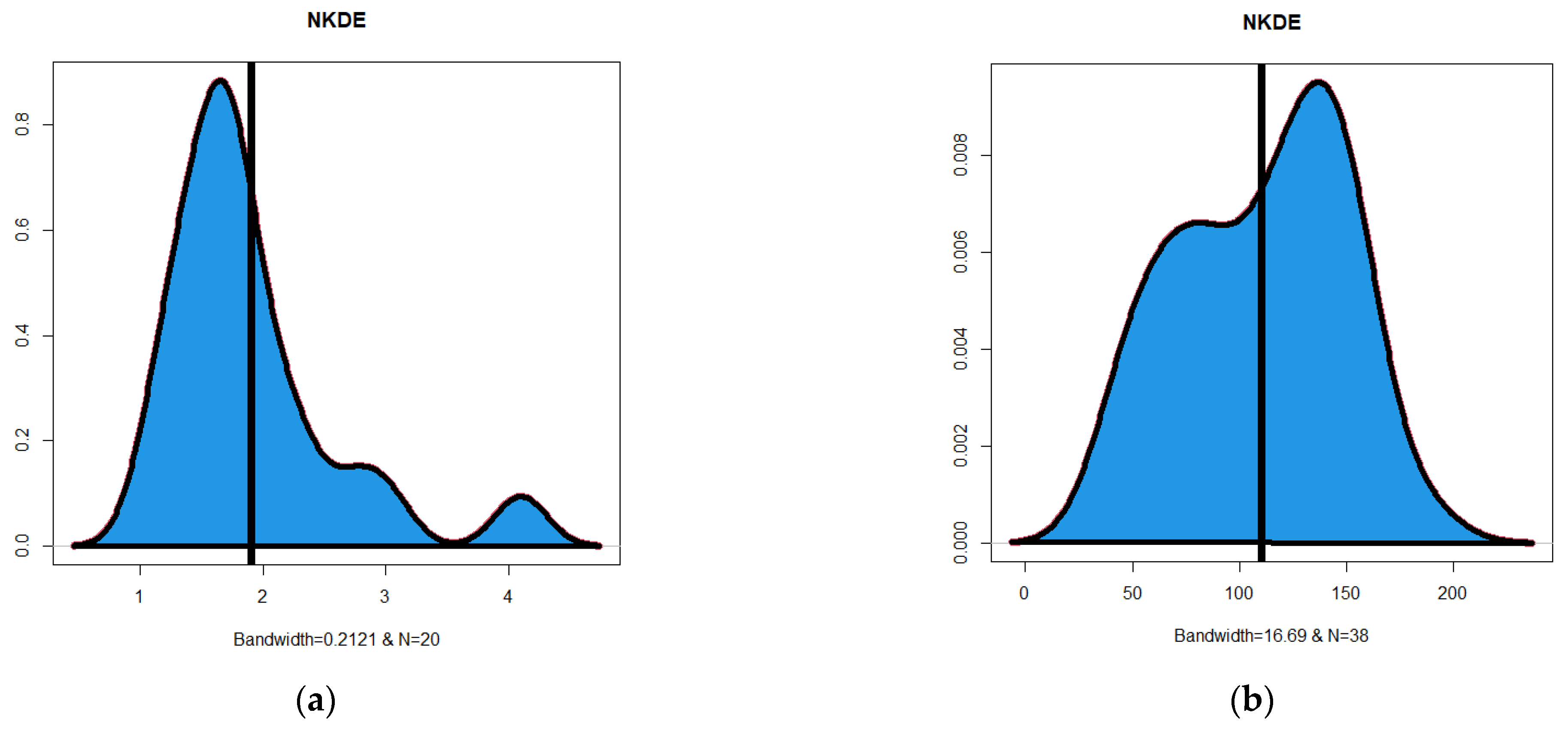
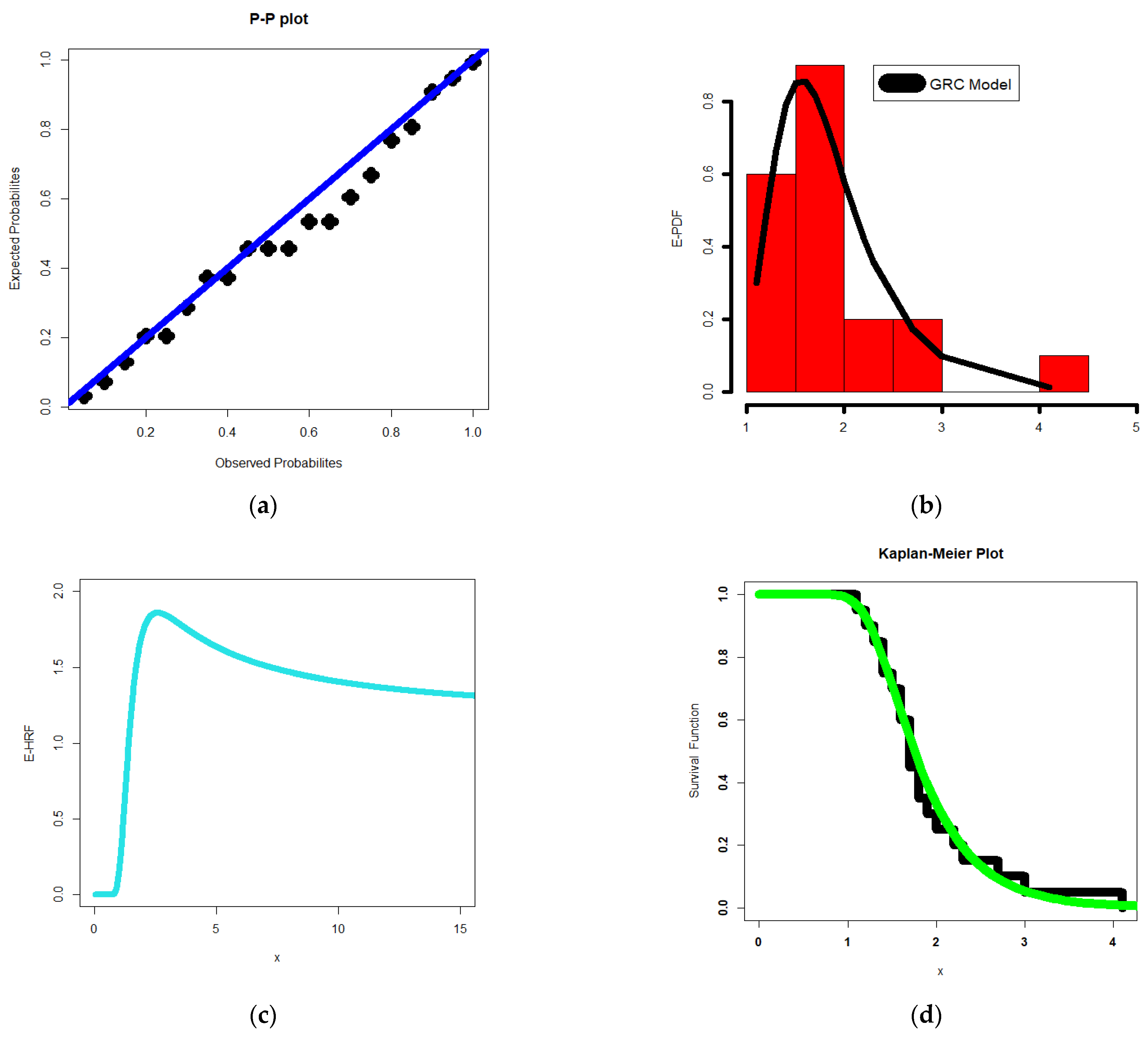
5. Applications for Asymmetrical Bimodal Data

Two actual data sets are examined and taken into account in this part using the maximum likelihood estimation (MLE) approach to demonstrate the applicability of the GRC model. The Akaike Information Criteria (AIC), Consistent Akaike Information Criteria (CAIC), Bayesian Akaike Information Criteria (BAIC), the Cramér–Von Mises test (CVMT), and the Anderson–Darling Criteria (ADC) are some of the criteria we take into consideration while evaluating models. The Kolmogorov–Smirnov (K.S) test and associated p-value (p-v) are also carried out. The MLE approach has been used to estimate model parameters. The relief times of data of 20 patients are included in the first data set (1.1, 1.3, 1.4, 1.7, 1.8, 1.6, 1.9, 2.2, 1.7, 4.1, 2.7, 1.8, 1.2, 1.4, 1.5, 3, 1.7, 1.6, 2, 2.3). The second set of data is referred to as the minimum flow and includes the following values: 43.86, 44.97, 46.27, 51.29, 61.19, 61.20, 67.80, 69.00, 71.84, 77.31, 85.39, 86.59, 86.66, 88.16, 96.03, 102.00, 108.29, 113.00, 115.14, 116.71, and 126.00. Table 1 gives the results of the comparing models under the relief data set. Table 2 provides the MLEs and SEs for the relief data set. Table 3 gives the results of comparing the models under the flow data set. Table 4 lists the MLEs and SEs for the minimum flow data. Utilizing the relief times real data set, Table 1 presents statistical tests for contrasting the competing Chen extensions. The MLEs and associated standard errors (SEs) for the relief times real data set are listed in Table 2. The competing Chen extensions are represented in Table 1 and Table 2 as the GRC (the proposed model), Gamma-Chen (GC), Kumaraswamy Chen (KUMC), Beta-Chen (BC), Marshall–Olkin Chen (MOC), Transmuted Chen (TC), and traditional two-parameters Chen. Table 3 offers statistical tests for contrasting the competing models using the minimal flow data set. Table 4 contains a list of the MLEs and SEs for the minimal flow data set. The two real data sets are presented using box charts, quantile–quantile (Q–Q), total time in test (TTT), and nonparametric kernel density estimation (NKDE) plots.

Table 1. Comparing results using the relief data set.

Model	BIC	AIC	ADC	CVMT	p-Value	K.S
GRC	40.492	37.505	0.2321	0.0402	0.9524	0.1155
EWC	40.624	37.632	0.2411	0.042	0.9525	0.116
GC	50.335	46.353	0.2845	0.046	<0.013	0.992
BC	44.493	40.517	0.348	0.065	0.7688	0.155
TC	56.625	53.635	1.576	0.274	0.2427	0.233
KUMC	44.324	40.024	0.303	0.059	0.8200	0.140
MOC	47.877	44.879	0.848	0.147	0.7738	0.157
Chen	55.129	53.144	1.6666	0.297	0.2055	0.244

Table 2. The MLEs and their corresponding SEs for the relief data set.

Model	MLE (SEs)
$\mathrm{GRC}(\alpha ,\theta ,\beta$)	$1.097\times {10}^3$$,9.222\times {10}^{-2}$$,7.028\times {10}^{-1}$
	$(1.640\times {10}^3$$),(2.467\times {10}^{-2}$$),(5.39\times {10}^{-2}$)
$\mathrm{EWC}(\alpha ,\theta ,\beta$)	1663.342, 1.1672, 0.1213
	(3.863), (2.4872), (5.7591)
$\mathrm{GC}(\mathsf{\gamma },\alpha ,\theta ,\beta$)	7.5914, 1.988, 5.0023, 0.534
	(2.091), (0.462), (1.077), (0.0030)
$\mathrm{MOC}(\alpha ,\theta ,\beta$)	400.01231, 2.32433, 0.4343
	(488.0654), (0.643), (0.082)
$\mathrm{KUMC}(\mathsf{\gamma },\alpha ,\theta ,\beta$)	160.07, 0.491, 2.212, 0.5234
	(222.413), (0.514), (0.752), (0.214)
$\mathrm{BC}(\mathsf{\gamma },\alpha ,\theta ,\beta$)	85.873, 0.481, 2.013, 0.552
	(103.1), (0.512), (0.69), (0.202)
$\mathrm{TC}(\alpha ,\theta ,\beta$)	0.74554, 0.07144, 1.0221
	(0.2841), (0.034), 0.09)
$\mathrm{Chen}(\theta ,\beta$)	0.13888, 0.9453
	(0.05121, 0.093)

Table 3. Comparing models under the flow data set.

Model	BIC	AIC	ADC	CVMT	p-Value	K.S
GRC	394.349	389.436	0.443	0.054 5	0.7617	0.1086
EWC	394.373	389.360	0.6021	0.1198	0.7050	0.1133
MOC	395.471	390.563	0.6111	0.0930	0.6892	0.1239
GC	398.033	391.480	1.7112	0.2888	<0.010	0.5735
Chen	401.900	398.623	0.6465	0.1014	0.2623	0.1665
BC	398.761	392.210	0.7532	0.1219	0.343	0.1542
KUMC	397.788	391.236	0.6664	0.1191	0.4090	0.1451
TEC	398.290	391.735	0.7054	0.1111	0.3728	0.1549
TC	394.444	389.533	0.6632	0.1132	0.3825	0.1555
EC	394.818	389.912	0.7223	0.1312	0.3488	0.1513

Table 4. The MLEs and SEs for the minimum flow data.

Model	MLE (SEs)
$\mathrm{GRC}(\alpha ,\theta ,\beta$)	0.5443, 0.3596,8 0.0017
	(0.0938), (0.002), (0.013)
$\mathrm{GRC}(\alpha ,\theta ,\beta$)	19.79869, 0.05371, 0.24494
	(4.666), (0.0049), (0.00363)
$\mathrm{BC}(\mathsf{\gamma },\alpha ,\theta ,\beta$)	3.0143, 0.7741, 0.014, 0.3542
	(1.9013), (1.244), (0.011), (0.051)
$\mathrm{KUMC}(\mathsf{\gamma },\alpha ,\theta ,\beta$)	4.514, 21.1104, 0.022, 0.273
	(2.022), (42.855), (0.02), (0.054)
$\mathrm{GC}(\mathsf{\gamma },\alpha ,\theta ,\beta$)	3.1353, 4.364, 0.096, 0.345
	(1.143), (4.4), (0.02), (0.02)
$\mathrm{MOC}(\alpha ,\theta ,\beta$)	13.0014, 0.0232, 0.3454
	(18.666), (0.024), (0.044)
$\mathrm{EC}(\alpha ,\theta ,\beta$)	2.85937, 0.01443, 0.3553
	(0.9832), (0.0045), (0.0234)
$\mathrm{TEC}(\mathsf{\gamma },\alpha ,\theta ,\beta$)	2.737, −0.248, 0.01, 0.348
	(1.213), (0.466), (0.013), (0.023)
$\mathrm{TC}(\alpha ,\theta ,\beta$)	−1.00442, 0.00394, 0.3684
	(0.702), (0.002), (0.012)
$\mathrm{Chen}(\theta ,\beta$)	0.00323, 0.3654
	(0.00113), 0.0133)

These Q–Q plots are shown in Figure 3. In Figure 4, the TTT graphs are displayed. The NKDE graphs are shown in Figure 5. The Q–Q shows that the first data have some extreme values. The TTT plot shows that the HRFs for the two data sets are “monotonically increasing”. The KDE of the minimum flow data is “asymmetric bimodal density” with a right tail, as shown by the NKDE plot (see Figure 5a). The KDE of the relief data is “asymmetric bimodal density” (see Figure 5b).

Figure 3. Q–Q plots.

Figure 4. TTT plots.

Figure 5. (a) The NKDE plot for the relief times data with suitable bandwidth, and (b) the NKDE plot for the minimum flow data with suitable bandwidth.

Table 1 indicates that the GRC model yields the best outcomes: AIC = 37.505, BIC = 40.492, CVM = 0.402, AD = 0.2321, K.S = 0.1515, and p = 9524. The MLEs (SEs) for the relief periods data are shown in Table 3. Table 3 indicates that the GRC model yields the best outcomes: AIC = 389.436, BIC = 394.349, CVM = 0.0545, AD = 0.443, K.S = 0.1106, and p = 766.

For the relief periods and lowest flow data sets, Figure 6 and Figure 7 show the probability–probability (P–P), estimated-PDF (E-PDF), estimated-HRF (E-HRF), and the Kaplan–Meier survival plot, respectively.

Figure 6. The P–P (a); E-PDF (b); E-HRF (c); Kaplan–Meier plot (d); for the relief times data.

Figure 7. The P–P (a); E-PDF (b); E-HRF (c) Kaplan–Meier plot (d); for the minimum flow data.

Figure 6 and Figure 7 indicate that the new model successfully modelled the relief timings and minimum flow data sets while fitting the empirical functions quite closely.

6. Risk Analysis

6.1. Risk Analysis under Artificial Experiments

For risk analysis and evaluation, the maximum likelihood, weighted least squares, ordinary least squares, Cramér–von Mises, moments, and Anderson–Darling approaches are considered. We will ignore the algebraic derivations and theoretical results of these methods since it is already present in a lot of the statistical literature. On the other hand, we will focus a lot on the practical results and statistical applications of mathematical modeling in general and of the risk disclosure, analysis risk, and evaluation of actuarial risks. For computing the abovementioned KRIs, the following estimation techniques are discussed in these sections: the MLE method, the OLS method, the WLSE method, and the ADE method. Six CLs (q = 60, 70, 90, 95, 99, and 99.9%) and N = 1000 with various sample sizes (n = 20, 50, 150, 300, 500) are considered under ${\alpha }_0=2, {\theta }_0=0.5, {\beta }_0=0.7$. All results are reported in Table A1, Table A2, Table A3 and Table A4. Table A1 gives the KRIs for the GRC under artificial data where n = 50. Table A2 shows the KRIs for the GRC under artificial data where n = 150. Table A3 lists the KRIs for the GRC under artificial data where n = 300. Table A4 provides the KRIs for the GRC under artificial data where n = 500. The simulation’s primary objective is to evaluate the efficacy of the four risk analysis methodologies and select the most appropriate and efficient ones. Table A1, Table A2, Table A3, Table A4 and Table A5 allow us to display the significant conclusions:

• The $\mathrm{VAR}$($X;\widehat{\underset{\_}{V}}$), $\mathrm{TVAR}\left(X;\widehat{\underset{\_}{V}}\right),$ and $\mathrm{TMV}\left(X;\widehat{\underset{\_}{V}},0.5\right)$ increase when q increases for all estimation methods.
• The $\mathrm{TV}\left(X;\widehat{\underset{\_}{V}}\right)$ and $\mathrm{MEL}\left(X;\widehat{\underset{\_}{V}}\right)$ decrease when q increases for all estimation methods.
• The results of the four tables allow us to confirm that all methods work properly and that it is impossible to clearly advocate one strategy over another. We are required to create an application based on real data considering this basic discovery in the hopes that it will help us choose one approach over another and identify the best and most relevant ways. In other words, while the four approaches gave us comparable findings in risk assessment, the simulation research did not assist us in deciding how to weight the methodologies. These convergent findings reassure us that all techniques perform well and within acceptable limits when modelling actuarial data and assessing risk. More specifically, some main results can be highlighted due to Table A1, Table A2, Table A3, Table A4 and Table A5.

Based on Table A1, we conclude that it is not easy to determine the best way to assess and analyze risks where n = 20. It can be said (in general) that in the case of small samples, all estimation methods help in the risk assessment processes in close proximity to each other. Based on Table A2, we conclude that it is not easy to determine the best way to assess and analyze risks where n = 50. It can be said (in general) that in the case of small samples, all estimation methods help in the risk assessment processes in close proximity to each other. However, based on Table A3 (for n = 150), we conclude that the MLE is the best method for all risk indicators, for example VAR$\left(X;\widehat{{\displaystyle \underset{\_}{V}}}\right)$ started with 0.577686|$60\%$ and ended with 1.125096|$99.9\%$. The same conclusions can be obtained for the other risk indicators. Based on Table A4 and Table A5 (for n = 300 and n = 500), we conclude that the moment method is the worst one; however, all other methods perform well. Table A1, Table A2, Table A3, Table A4 and Table A5 are given in Appendix A.

6.2. Risk Analysis for Insurance Claims Data

In this part, we use a U.K. motor non-comprehensive account as an example of the insurance claims payment triangle in this study for practical purposes. For the sake of convenience, we decide to place the origin period between 2007 and 2013 (see Mohamed et al. [4]). The claims data are presented in the insurance claims payment data frame in the same way that a database would typically store it. The first column lists the development year, the incremental payments, and the origin year, which spans from 2007 to 2013. It is vital to remember that a probability-based distribution was first used to analyze this data on insurance claims. Real data analysis can be performed numerically, graphically, or by fusing the two. When examining initial fits of theoretical distributions, such as the normal, uniform, exponential, logistic, beta, lognormal, Weibull, and the numerical technique, a few graphical tools, such as the skewness-kurtosis plot (or the Cullen and Frey plot), are taken into consideration (see Figure 8). Figure 8 depicts our left-skewed data with a kurtosis less than three. The initial shape of the insurance claims density is examined using the NKDE approach (see Figure 9a), the current data’s “normality” is examined using the Q–Q plot (see Figure 9b), the empirical HRF’s initial shape is examined using the TTT plot (see Figure 9c), and the explanatory variables are determined using the “box plot” (see Figure 9c,d).

Figure 8. Cullen–Frey plot for the actuarial claims data.

Figure 9. NKDE (a); Q–Q (b); TTT (c); box plots (d).

The initial density is depicted as an asymmetric function with a left tail in Figure 9a. Based on Figure 9, no outlandish assertions are apparent in Figure 9d. The HRF for the models that account for the present data should also be monotonically growing (see Figure 9c). The scattergrams for the data on insurance claims are shown in Figure 10. For the data on insurance claims, Figure 11a shows the autocorrelation function (ACF), and Figure 11b shows the partial autocorrelation function (partial ACF). We provide the ACF, which can be used to demonstrate how the correlation between any two signal values alters when the distance between them alters the ACF. The theoretical ACF is a time domain measure of the stochastic process memory and offers no insight into the frequency content of the process. With Lag = k = 1, it offers some details on the distribution of hills and valleys on the surface (see Figure 11a). Additionally included is the theoretical partial ACF with Lag = k = 1 (see Figure 11b). In contrast to the other partial autocorrelations for all other lags, the first lag value is shown in Figure 11b to be statistically significant. The initial NKDE has an asymmetric density with a left tail, as shown in Figure 9a. On the other hand, the interview, matching, and density of the novel model, which incorporates the left tail shape, are significant in statistical modelling. Therefore, it is advised to use the GRC model to simulate the payments for insurance claims. We present an application for risk analysis under VAR, TVAR, TV, TMV, and $\mathrm{EL}$ measures for the insurance claims data. The risk analysis is performed for some confidence level as follows:

$$q=60\%,70\%,80\%,90\%,95\%,99\%,\mathrm{and}99.9\%.$$

Figure 10. The scattergrams.

Figure 11. (a) The ACF plot for the insurance claims data, and (b) the partial ACF plot for the insurance claims data.

The five measures are estimated for the GRC and C models. Table 5 gives the KRIs for the GRC under insurance claims data. Table 6 lists the KRIs for the GRC under insurance claims data. Table 7 provides the estimators and ranks for the GRC model under the claims data for all estimation methods. Table 8 provides the estimators and ranks for the C model under the claims data for all estimation methods. Table 8 shows the estimators and ranks for the C model under the claims data for all estimation methods. The C distribution was chosen because it is the baseline distribution on which the new distribution is based. Based on these tables, the following results can be highlighted:

Table 5. The KRIs for the GRC under insurance claims data.

$\mathbf{Method}\downarrow$	$\mathbf{CL}\downarrow$	$\mathbf{VAR}\left(\mathit{X};\widehat{\underset{\_}{\mathit{V}}}\right)$	$\mathbf{TVAR}\left(\mathit{X};\widehat{\underset{\_}{\mathit{V}}}\right)$	$\mathbf{TV}\left(\mathit{X};\widehat{\underset{\_}{\mathit{V}}}\right)$	$\mathbf{TMV}\left(\mathit{X};\widehat{\underset{\_}{\mathit{V}}},0.5\right)$	$\mathbf{MEL}\left(\mathit{X};\widehat{\underset{\_}{\mathit{V}}}\right)$
MLE	$60\%$	2995.433059	4275.474776	1,042,528.782433	525,539.865993	1280.041717
	$70\%$	3468.400242	4625.137504	895,045.930997	452,148.103003	1156.737262
	$80\%$	4038.356035	5066.752664	744,038.824351	377,086.16484	1028.396629
	$90\%$	4846.834605	5723.310099	572,400.996532	291,923.808365	876.475495
	$95\%$	5521.447578	6292.299079	460,064.535012	236,324.566585	770.851502
	$99\%$	6781.639964	7399.960377	207,362.181718	111,081.051237	618.320413
	$99.9\%$	8156.146208	8635.322651	196,466.546046	106,868.595674	479.176442
LS	$60\%$	2995.79625	4823.79565	2,565,875.85054	1,287,761.72092	1827.9994
	$70\%$	3605.64058	5334.88391	2,366,027.27058	1,188,348.5192	1729.24334
	$80\%$	4391.41575	6013.29109	2,142,778.10812	1,077,402.34515	1621.87534
	$90\%$	5601.69265	7087.85952	1,856,663.30908	935,419.51407	1486.16688
	$95\%$	6697.28146	8081.14632	1,641,518.22068	828,840.25666	1383.86487
	$99\%$	8949.4202	10,160.16005	1,291,686.50067	656,003.41039	1210.73985
	$99.9\%$	11,699.26883	12,740.63136	977,455.63285	501,468.44778	1041.36252
WLS	$60\%$	2993.45166	4368.83178	1,198,197.19961	603,467.43158	1375.38011
	$70\%$	3502.27954	4744.4535	1,026,058.03873	517,773.47286	1242.17396
	$80\%$	4115.72289	5218.34142	849,786.00448	430,111.34366	1102.61853
	$90\%$	4984.46424	5921.19761	649,727.92329	330,785.15925	936.73337
	$95\%$	5707.04377	6528.38195	519,378.08162	266,217.42276	821.33818
	$99\%$	7050.06113	7698.10238	342,283.93764	178,840.0712	648.04125
	$99.9\%$	8505.4338	9010.49496	217,699.48623	117,860.23808	505.06116
CVM	$60\%$	2975.27503	4684.45314	2,201,083.89688	1,105,226.40158	1709.1781
	$70\%$	3551.76054	5161.13256	2,017,075.48552	1,013,698.87532	1609.37202
	$80\%$	4289.09745	5790.95426	1,812,296.77407	911,939.34129	1501.85681
	$90\%$	5415.39634	6782.63414	1,554,382.10192	783,973.6851	1367.2378
	$95\%$	6427.2668	7694.09081	1,363,501.38182	689,444.78172	1266.82401
	$99\%$	8489.86108	9589.04377	1,057,767.93624	538,473.01189	1099.18269
	$99.9\%$	10,984.15414	11,922.07451	789,278.32307	406,561.23605	937.92037
ADE	$60\%$	2977.72629	4499.40165	1,593,652.26016	801,325.53173	1521.67536
	$70\%$	3516.26365	4919.35247	1,411,403.46935	710,621.08715	1403.08883
	$80\%$	4184.76712	5461.36406	1,217,267.95014	614,095.33913	1276.59695
	$90\%$	5167.3597	6289.28735	984,627.83405	498,603.20438	1121.92765
	$95\%$	6016.03503	7026.48158	823,529.60842	418,791.28579	1010.44655
	$99\%$	7665.33888	8499.81389	586,821.22316	301,910.42547	834.475
	$99.9\%$	9548.8129	10,227.62167	402,428.42768	211,441.83551	678.80877
Moment	$60\%$	2938.57331	4201.12314	1,050,991.15004	529,696.69817	1262.54983
	$70\%$	3396.72068	4547.52614	915,340.92543	462,217.98885	1150.80546
	$80\%$	3955.16777	4989.23409	774,776.31709	392,377.39264	1034.06633
	$90\%$	4759.76904	5654.47064	611,475.60507	311,392.27317	894.7016
	$95\%$	5442.35853	6238.90719	501,528.1582	257,002.98629	796.54866
	$99\%$	6743.48259	7388.89619	346,141.988	180,459.89019	645.4136
	$99.9\%$	8197.24619	8712.92223	229,937.55821	123,681.70134	515.67604

Table 6. The KRIs for the C model under insurance claims data.

$\mathbf{Method}\downarrow$	$\mathbf{CL}\downarrow$	$\mathbf{VAR}\left(\mathit{X};\widehat{\underset{\_}{\mathit{V}}}\right)$	$\mathbf{TVAR}\left(\mathit{X};\widehat{\underset{\_}{\mathit{V}}}\right)$	$\mathbf{TV}\left(\mathit{X};\widehat{\underset{\_}{\mathit{V}}}\right)$	$\mathbf{TMV}\left(\mathit{X};\widehat{\underset{\_}{\mathit{V}}},0.5\right)$	$\mathbf{MEL}\left(\mathit{X};\widehat{\underset{\_}{\mathit{V}}}\right)$
MLE	$60\%$	3018.151137	4228.504423	895,307.42374	451,882.216293	1210.353286
	$70\%$	3476.191406	4557.144289	755,914.936649	382,514.612614	1080.952883
	$80\%$	4018.195081	4967.151113	617,382.044371	313,658.173299	948.956032
	$90\%$	4771.39211	5568.556439	448,149.30637	229,643.209624	797.16433
	$95\%$	5388.71247	6083.137469	369,667.951793	190,917.113365	694.424999
	$99\%$	6523.604751	7069.40067	243,602.679891	128,870.740616	545.795919
	$99.9\%$	7749.241041	8177.125483	157,453.697061	86,903.974013	427.884442
LS	$60\%$	3057.31723	4616.08258	1,572,944.00665	791,088.08591	1558.76535
	$70\%$	3627.94661	5042.87182	1,359,642.80998	684,864.27681	1414.92521
	$80\%$	4320.48304	5584.35879	1,139,971.02561	575,569.8716	1263.87575
	$90\%$	5309.58291	6393.90828	889,164.50728	450,976.16192	1084.32537
	$95\%$	6140.27802	7100.03757	724,434.88826	369,317.4817	959.75955
	$99\%$	7707.47013	8481.07818	498,718.1162	257,840.13628	773.60805
	$99.9\%$	9449.44305	10,070.24175	335,705.12524	177,922.80437	620.7987
WLS	$60\%$	3016.57287	4357.54867	1,125,040.18728	566,877.64231	1340.97581
	$70\%$	3517.26542	4722.90662	959,163.35091	484,304.58208	1205.6412
	$80\%$	4115.89338	5181.88499	791,913.74316	401,138.75657	1065.99161
	$90\%$	4957.14659	5860.26126	605,455.00866	308,587.76559	903.11467
	95%	5653.57081	6445.60633	485,959.42745	249,425.32005	792.03552
	$99\%$	6947.55125	7576.56834	325,971.49602	170,562.31636	629.01709
	$99.9\%$	8361.65005	8859.53398	214,308.30495	116,013.68646	497.88393
CVM	$60\%$	3042.58341	4571.44196	1,507,415.34803	758,279.11598	1528.85855
	$70\%$	3603.50313	4989.81522	1,301,028.07761	655,503.85402	1386.31208
	80%	4283.12424	5520.04414	1,088,976.79416	550,008.44122	1236.9199
	$90\%$	5252.03564	6311.76547	847,325.32097	429,974.42596	1059.72983
	$95\%$	6064.47679	7001.50331	689,362.44601	351,682.72631	937.02652
	$99\%$	7594.63827	8348.70189	472,931.24023	244,814.322	754.06362
	$99.9\%$	9292.25602	9896.43605	317,706.23491	168,749.55351	604.18003
ADE	$60\%$	3025.58204	4382.96196	1,155,270.56969	582,018.24681	1357.37992
	$70\%$	3531.75877	4752.90735	985,824.9595	497,665.3871	1221.14858
	$80\%$	4137.52807	5217.94783	814,745.39537	412,590.64551	1080.41976
	$90\%$	4989.70807	5905.79682	623,720.17381	317,765.88372	916.08875
	$95\%$	5695.83725	6499.7418	501,000.37295	256,999.92827	803.90455
	$99\%$	7009.15169	7648.20733	336,694.11449	175,995.26458	639.05564
	$99.9\%$	8445.96804	8952.25142	221,709.26206	119,806.88245	506.28338
Moment	60%	966.65702	4103.34393	13,926,896.58904	6,967,551.63844	3136.68691
	$70\%$	1653.56101	5043.53049	15,020,357.32578	7,515,222.19338	3389.96948
	$80\%$	2811.11642	6476.60327	16,314,187.9627	8,163,570.58462	3665.48685
	90%	5145.63806	9139.30372	18,006,882.83894	9,012,580.72319	3993.66566
	$95\%$	7776.40195	11,987.80281	19,224,262.08164	9,624,118.84363	4211.40085
	$99\%$	14,529.11205	19,024.55224	20,916,418.13409	10,477,233.61929	4495.4402
	$99.9\%$	24,938.9476	29,594.42541	21,896,109.43017	10,977,649.14049	4655.47781

Table 7. The estimators and ranks for the GRC model under the claims data for all estimation methods.

$\mathbf{Estimates}\mathbf{and}\mathbf{Rank}\to$ $\mathbf{Methods}\downarrow$	$\widehat{\mathit{\alpha }}$	$\widehat{\mathit{\theta }}$	$\widehat{\mathit{\beta }}$	Rank
MLE	1.52776	0.15012	0.02804	6
LS	2.31433	0.11868	0.06689	1
WLS	1.34353	0.15026	0.02708	4
CVM	2.3485	0.12133	0.06332	2
ADE	0.17658	0.13559	0.04256	3
Moment	2.17018	0.14186	0.03780	5

Table 8. The estimators and ranks for the C model under insurance claims data for all estimation methods.

$\mathbf{Estimates}\mathbf{and}\mathbf{Rank}\to$ $\mathbf{Methods}\downarrow$	$\widehat{\mathit{\theta }}$	$\widehat{\mathit{\beta }}$	Rank
MLE	0.25197	0.00049	6
LS	0.23566	0.00121	2
WLS	0.24496	0.00074	5
CVM	0.23669	0.00116	3
ADE	0.24429	0.00077	4
Moment	0.15750	0.05048	1

1. For all risk assessment methods|$q=60, 70, 80, 90, 95, 99,\mathrm{and}99.9\%$:

$$\mathrm{VAR}\left(X;\underset{\_}{V}\right){|}_{q=60\%}<\mathrm{VAR}\left(X;\underset{\_}{V}\right){|}_{q=70\%}\dots <\mathrm{VAR}\left(X;\underset{\_}{V}\right){|}_{q=99.9\%}.$$

2. For all risk assessment methods|$q=60, 70, 80, 90, 95, 99,\mathrm{and}99.9\%$:

$$\mathrm{TVAR}\left(X;\underset{\_}{V}\right){|}_{q=60\%}<\mathrm{TVAR}\left(X;\underset{\_}{V}\right){|}_{q=70\%}\dots <\mathrm{TVAR}\left(X;\underset{\_}{V}\right){|}_{q=99.9\%}.$$

3. For Most risk assessment methods|$q=60,70,80,90,95,99,\mathrm{and}99.9\%$:

$$\mathrm{TV}\left(X;\underset{\_}{V},0.5\right){|}_{q=60\%}<\mathrm{TV}\left(X;\underset{\_}{V},0.5\right){|}_{q=70\%}\dots <\mathrm{TV}\left(X;\underset{\_}{V},0.5\right){|}_{q=99.9\%}.$$

4. For all risk assessment methods|$q=60,70,80,90,95,99,\mathrm{and}99.9\%$:

$$\mathrm{TMV}\left(X;\underset{\_}{V},0.5\right){|}_{q=60\%}>\mathrm{TMV}\left(X;\underset{\_}{V},0.5\right){|}_{q=70\%}\dots >\mathrm{TMV}\left(X;\underset{\_}{V},0.5\right){|}_{q=99.9\%}.$$

5. For all risk assessment methods|$q=60, 70, 80, 90, 95, 99,\mathrm{and}99.9\%$:

$$\mathrm{MEL}\left(X;\underset{\_}{V},0.5\right){|}_{q=60\%}>\mathrm{MEL}\left(X;\underset{\_}{V},0.5\right){|}_{q=70\%}\dots >\mathrm{MEL}\left(X;\underset{\_}{V},0.5\right){|}_{q=99.9\%}.$$

6. Under the GRC model and the MLE method, the VAR($X;\widehat{\underset{\_}{V}}$) is a monotonically increasing indicator starting with 2995.433059 ${|}_{q=60\%}$ and ending with 8156.146208${|}_{q=99.9\%}$. The TVAR($X;\widehat{\underset{\_}{V}}$) in a monotonically increasing indicator starts with 4275.474776${|}_{q=60\%}$ and ends with 4275.474776${|}_{q=99.9\%}$. However, the TV($X;\widehat{\underset{\_}{V}}$), the TMV($X;\widehat{\underset{\_}{V}}$), and the MEL($X;\widehat{\underset{\_}{V}}$) are monotonically decreasing.

7. Under the GG model and the MLE method, the VAR($X;\widehat{\underset{\_}{V}}$) is a monotonically increasing indicator starting with 3018.151137 ${|}_{q=60\%}$ and ending with 7749.241041${|}_{q=99.9\%}$. The TVAR($X;\widehat{\underset{\_}{V}}$) in a monotonically increasing indicator starts with 4228.504423 ${|}_{q=60\%}$ and ends with 8177.125483${|}_{q=99.9\%}$. The TV($X;\widehat{\underset{\_}{V}}$), the TMV($X;\widehat{\underset{\_}{V}}$), and the MEL($X;\widehat{\underset{\_}{V}}$) are monotonically decreasing indicators.

8. Under the GRC model and the LS method, the VAR($X;\widehat{\underset{\_}{V}}$) is a monotonically increasing indicator starting with 2995.79625${|}_{q=60\%}$ and ending with 11,699.26883${|}_{q=99.9\%}$. The TVAR($X;\widehat{\underset{\_}{V}}$) in a monotonically increasing indicator starts with 4823.79565 ${|}_{q=60\%}$ and ends with 12,740.63136${|}_{q=99.9\%}$. However, the TV($X;\widehat{\underset{\_}{V}}$), the TMV($X;\widehat{\underset{\_}{V}}$), and the ($X;\widehat{\underset{\_}{V}}$) are monotonically decreasing.

9. Under the GG model and the OLSE method, the VAR($X;\widehat{\underset{\_}{V}}$) is a monotonically increasing indicator starting with 3057.31723${|}_{q=60\%}$ and ending with 9449.44305${|}_{q=99.9\%}$. The TVAR($X;\widehat{\underset{\_}{V}}$) in a monotonically increasing indicator starts with 4616.08258${|}_{q=60\%}$ and ends with 10,070.24175${|}_{q=99.9\%}$. However, the TV ($X;\widehat{\underset{\_}{V}}$), the TMV ($X;\widehat{\underset{\_}{V}}$), and the MEL($X;\widehat{\underset{\_}{V}}$) are monotonically decreasing.

10. Under the GRC model and the WLSE method, the VAR($X;\widehat{\underset{\_}{V}}$) is a monotonically increasing indicator starting with 2993.45166${|}_{q=60\%}$ and ending with 8505.4338${|}_{q=99.9\%}$. The TVAR($X;\widehat{\underset{\_}{V}}$) in a monotonically increasing indicator starts with 4368.83178${|}_{q=60\%}$ and ends with 9010.49496${|}_{q=99.9\%}$. However, the TV($X;\widehat{\underset{\_}{V}}$), the TMV($X;\widehat{\underset{\_}{V}}$), and the MEL($X;\widehat{\underset{\_}{V}}$) are monotonically decreasing.

11. Under the GG model and the WLSE method, the VAR($X;\widehat{\underset{\_}{V}}$) is a monotonically increasing indicator starting with 8361.65005${|}_{q=60\%}$ and ending with 8859.53398${|}_{q=99.9\%}$. The TVAR($X;\widehat{\underset{\_}{V}}$) in a monotonically increasing indicator starts with 4357.54867${|}_{q=60\%}$ and ends with 8859.53398${|}_{q=99.9\%}$. However, the TV($X;\widehat{\underset{\_}{V}}$), the TMV($X;\widehat{\underset{\_}{V}}$), and the MEL($X;\widehat{\underset{\_}{V}}$) are monotonically decreasing.

12. Under the GRC model and the CVM method, the VAR($X;\widehat{\underset{\_}{V}}$) is a monotonically increasing indicator starting with 2975.27503${|}_{q=60\%}$ and ending with 10,984.15414${|}_{q=99.9\%}$. The TVAR($X;\widehat{\underset{\_}{V}}$) in a monotonically increasing indicator starts with 4684.45314${|}_{q=60\%}$ and ends with 11,922.07451${|}_{q=99.9\%}$. However, the TV($X;\widehat{\underset{\_}{V}}$), the TMV($X;\widehat{\underset{\_}{V}}$), and the MEL($X;\widehat{\underset{\_}{V}}$) are monotonically decreasing.

13. Under the GG model and the AE method, the VAR($X;\widehat{\underset{\_}{V}}$) is a monotonically increasing indicator starting with 3042.58341${|}_{q=60\%}$ and ending with 9292.25602${|}_{q=99.9\%}$. The TVAR($X;\widehat{\underset{\_}{V}}$) in a monotonically increasing indicator starts with 4571.44196${|}_{q=60\%}$ and ends with 9896.43605${|}_{q=99.9\%}$. However, the TV($X;\widehat{\underset{\_}{V}}$), the TMV($X;\widehat{\underset{\_}{V}}$), and the MEL($X;\widehat{\underset{\_}{V}}$) are monotonically decreasing.

14. Under the GRC model and the ADE method, the VAR($X;\widehat{\underset{\_}{V}}$) is a monotonically increasing indicator starting with 2977.72629${|}_{q=60\%}$ and ending with 9548.8129${|}_{q=99.9\%}$. The TVAR($X;\widehat{\underset{\_}{V}}$) in a monotonically increasing indicator starts with 4499.40165 ${|}_{q=60\%}$ and ends with 10,227.62167${|}_{q=99.9\%}$. However, the TV($X;\widehat{\underset{\_}{V}}$), the TMV($X;\widehat{\underset{\_}{V}}$), and the MEL($X;\widehat{\underset{\_}{V}}$) are monotonically decreasing.

15. Under the GG model and the AE method, the VAR($X;\widehat{\underset{\_}{V}}$) is a monotonically increasing indicator starting with 3025.58204${|}_{q=60\%}$ and ending with 8445.96804${|}_{q=99.9\%}$. The TVAR($X;\widehat{\underset{\_}{V}}$) in a monotonically increasing indicator starts with 4382.96196${|}_{q=60\%}$ and ends with 8952.25142${|}_{q=99.9\%}$. However, the TV($X;\widehat{\underset{\_}{V}}$), the TMV($X;\widehat{\underset{\_}{V}}$), and the MEL($X;\widehat{\underset{\_}{V}}$) are monotonically decreasing.

16. Under the GRC model and the moment method, the VAR($X;\widehat{\underset{\_}{V}}$) is a monotonically increasing indicator starting with 2938.57331${|}_{q=60\%}$ and ending with 8197.24619${|}_{q=99.9\%}$. The TVAR($X;\widehat{\underset{\_}{V}}$) in a monotonically increasing indicator starts with 4201.12314${|}_{q=60\%}$ and ends with 8712.92223${|}_{q=99.9\%}$. However, the TV($X;\widehat{\underset{\_}{V}}$), the TMV($X;\widehat{\underset{\_}{V}}$), and the MEL($X;\widehat{\underset{\_}{V}}$) are monotonically decreasing.

17. Under the GG model and the AE method, the VAR($X;\widehat{\underset{\_}{V}}$) is a monotonically increasing indicator starting with 966.65702${|}_{q=60\%}$ and ending with 24,938.9476${|}_{q=99.9\%}$. The TVAR($X;\widehat{\underset{\_}{V}}$) in a monotonically increasing indicator starts with 4103.34393 ${|}_{q=60\%}$ and ends with 29,594.42541${|}_{q=99.9\%}$. However, the TV($X;\widehat{\underset{\_}{V}}$), the TMV($X;\widehat{\underset{\_}{V}}$), and the MEL($X;\widehat{\underset{\_}{V}}$) are monotonically decreasing.

18. For the GRC model, the OLSE approach is recommended since it offers the most acceptable risk exposure analysis, followed by the CVME method, and finally the ADE method. The other three techniques work well, though.

19. For the GG model, the moment technique is suggested for all q values since it offers the most acceptable risk exposure analysis. The LSE method is suggested next as a backup, and finally the CVME approach. The other three techniques work nicely, though.

20. The GRC model performs better than the GG model for all q values and for all risk methodologies. The new distribution performs the best when modelling insurance claims reimbursement data and determining actuarial risk, despite the fact that the probability distributions have the same number of parameters. In upcoming actuarial and applied research, we anticipate that actuaries and practitioners will be very interested in the new distribution.

6.3. Quantitative Risk Analysis Based on the Quantiles

To compare the effectiveness of the estimators of VAR based on the quantiles of the proposed GRC distribution, it is recommended to apply the Peaks Over Random Threshold (PORT) Mean-of-Order-p (MOp) methodology. However, in this work, we present a simulation analysis in this section. In order to compare the performance of the proposed distribution, we conduct a simulation study. Here, we consider two cases of sample generation. First, we generate samples of size n, (n = 50, 200, 500, 1000), for selected parameter values of the Chen and then from the proposed GRC distributions. In each case, our interest is to compare the estimation of two basic parameters of the Chen, β and θ, using the maximum likelihood method. Recall that all the other distributions are variants of the Chen distribution, and hence, it is natural that we can check how well the two parameters of the Chen distribution are estimated by the other variants. In addition, we assess the performance using the metrics, mean square error, and bias. Table 9, Table 10, Table 11 and Table 12 show the results of the simulation study for samples of different sizes generated from the Chen distribution with parameters β = 1.25 and θ = 0.75. The estimators of the two parameters from the MOC and GC are the most appropriate as they have less bias and MSE values. In addition, the proposed GRC estimator has smaller bias and MSE values in the estimation of θ than the Chen estimator. On the other hand, in the case of the estimation of β, the Chen estimator is better.

Table 9. Results for samples generated from the Chen distribution with n = 50.

$\mathbf{Distribution}\mathbf{and}\mathbf{Bias}\downarrow$
Estimator	Chen	GRC	GC	KUMC	MOC	TEC
$\widehat{\alpha }$	-	0.7821	1.14740	252.8311	1.8194	3.1188
$\widehat{\beta }$	0.1020	0.8678	0.29340	90.97970	0.2563	2.2633
$\widehat{\theta }$	1.4172	0.0437	0.01265	0.094400	0.0047	2.5657
$\widehat{a}$	-	-	-	308.0258	-	30.4398
$\widehat{b}$	-	-	-	76.06600	-	-
Distribution and bias$\downarrow$
Estimator	Chen	GRC	GC	KUMC	MOC	TEC
$\widehat{\alpha }$	-	−0.7662	−0.9539	15.9007	−1.0547	−1.766
$\widehat{\beta }$	−0.3125	−0.9316	−0.0095	9.5383	−0.0565	−1.5009
$\widehat{\theta }$	−1.1904	−0.2053	0.0195	−0.3067	0.0247	1.6018
$\widehat{a}$	-	-	-	17.5507	-	5.5172
$\widehat{b}$	-	-	-	8.7156	-	-

Table 10. Results for samples generated from the Chen distribution with n = 200.

$\mathbf{Distribution}\mathbf{and}\mathbf{MSE}\downarrow$
Estimator	Chen	GRC	GC	KUMC	MOC	TEC
$\widehat{\alpha }$	-	0.5537	0.6893	250.5503	1.0569	3.0902
$\widehat{\beta }$	0.1139	0.8768	0.0694	95.1393	0.0777	2.2738
$\widehat{\theta }$	1.4408	0.0446	0.0026	0.09490	0.0014	1.3801
$\widehat{a}$	-	-	-	305.5076	-	46.4741
$\widehat{b}$	-	-	-	85.5873	-	-
Distribution and bias$\downarrow$
Estimator	Chen	GRC	GC	KUMC	MOC	TEC
$\widehat{\alpha }$	-	−0.7441	−0.829	15.8287	−0.9145	−1.7579
$\widehat{\beta }$	−0.3375	−0.9364	0.02116	9.7539	−0.0459	−1.5079
$\widehat{\theta }$	−1.2003	−0.2106	0.0034	-0.3081	0.0113	1.1748
$\widehat{a}$	-	-	-	17.4787	-	6.8172
$\widehat{b}$	-	-	-	9.2513	-	-

Table 11. Results for samples generated from the Chen distribution with n = 500.

$\mathbf{Distribution}\mathbf{and}\mathbf{MSE}\downarrow$
Estimator	Chen	GRC	GC	KUMC	MOC	TEC
$\widehat{\alpha }$	-	0.6478	0.7424	247.2826	0.8578	3.0847
$\widehat{\beta }$	0.114	0.8663	0.0239	91.596	0.0362	2.2754
$\widehat{\theta }$	1.4408	0.0433	0.00077	0.0949	0.0005	1.0698
$\widehat{a}$	-	-	-	301.8983	-	82.8442
$\widehat{b}$	-	-	-	82.4628	-	-
Distribution and bias↓
Estimator	Chen	GRC	GC	KUMC	MOC	TEC
$\widehat{\alpha }$	-	−0.8049	−0.8616	15.7252	−0.898	−1.7563
$\widehat{\beta }$	−0.3376	−0.9308	−0.0054	9.5706	−0.0002	−1.5085
$\widehat{\theta }$	−1.2003	−0.208	0.0022	−0.3081	0.0041	1.0343
$\widehat{a}$	-	-	-	17.3752	-	9.1018
$\widehat{b}$	-	-	-	9.0809	-	-

Table 12. Results for samples generated from the Chen distribution with n = 1000.

$\mathbf{Distribution}\mathbf{and}\mathbf{MSE}\downarrow$
Estimator	Chen	GRC	GC	KUMC	MOC	TEC
$\widehat{\alpha }$	-	0.5236	0.6238	240.3421	0.6534	2.8015
$\widehat{\beta }$	0.1152	0.8663	0.0112	86.93	0.0196	2.2746
$\widehat{\theta }$	1.4414	0.0485	0.0004	0.0947	0.0003	0.8668
$\widehat{a}$	-	-	-	292.2038	-	127.32
$\widehat{b}$	-	-	-	80.3590	-	-
Distribution and bias$\downarrow$
Estimator	Chen	GRC	GC	KUMC	MOC	TEC
$\widehat{\alpha }$	-	−0.6216	−0.8507	15.444	−0.8859	−1.7497
$\widehat{\beta }$	−0.3395	−0.9307	0.0074	9.3236	−0.0072	−1.5082
$\widehat{\theta }$	−1.2006	−0.2202	0.0016	−0.3078	0.0009	0.9310
$\widehat{a}$	-	-	-	17.0939	-	11.283
$\widehat{b}$	-	-	-	8.9643	-	-

In the case of samples generated from the GRC distribution, the results are shown in Table 13, Table 14, Table 15 and Table 16. It can be observed that the estimation of β and θ from the GRC distribution offers the lowest bias and MSE in all cases. In addition, the estimators of the two distributions, GRC and Chen, show empirical consistency as the MSE decreases with increasing sample size.

Table 13. Results for samples generated from the GRC distribution with n = 50.

$\mathbf{Distribution}\mathbf{and}\mathbf{MSE}\downarrow$
Estimator	Chen	GRC	GC	KUMC	MOC	TEC
$\widehat{\alpha }$	-	0.2363	0.6892	832.8201	0.9754	1.3653
$\widehat{\beta }$	40.6931	0.0448	125.888	510.6551	46.1623	3.8990
$\widehat{\theta }$	0.02363	0.0022	0.6668	1.194900	0.1256	14.061
$\widehat{a}$	-	-	-	894.526	-	33.912
$\widehat{b}$	-	-	-	368.289	-	-
Distribution and bias$\downarrow$
Estimator	Chen	GRC	GC	KUMC	MOC	TEC
$\widehat{\alpha }$	-	−0.0991	−0.7347	28.8586	0.6776	−1.1685
$\widehat{\beta }$	6.3791	0.2115	11.22	22.5977	6.794283	1.9746
$\widehat{\theta }$	−0.1534	0.0192	0.8166	1.09310	0.3545	3.7498
$\widehat{a}$	-	-	-	29.9086	-	5.8234
$\widehat{b}$	-	-	-	19.1888	-	-

Table 14. Results for samples generated from the GRC distribution with n = 200.

$\mathbf{Distribution}\mathbf{and}\mathbf{MSE}\downarrow$
Estimator	Chen	GRC	GC	KUMC	MOC	TEC
$\widehat{\alpha }$	-	0.0486	0.45580	832.335	0.8829	1.3531
$\widehat{\beta }$	39.9115	0.0361	91.6124	521.084	47.0146	1.9761
$\widehat{\theta }$	0.02520	0.0004	0.52890	1.00610	0.1149	8.1882
$\widehat{a}$	-	-	-	894.023	-	18.522
$\widehat{b}$	-	-	-	366.152	-	-
Distribution and bias↓
Estimator	Chen	GRC	GC	KUMC	MOC	TEC
$\widehat{\alpha }$	-	−0.019	−0.6740	28.8502	0.9352	−1.1632
$\widehat{\beta }$	6.3176	0.1901	9.5714	22.8273	6.8567	1.4057
$\widehat{\theta }$	−0.1588	0.0090	0.7272	1.00300	0.339	2.8615
$\widehat{a}$	-	-	-	29.9002	-	4.3038
$\widehat{b}$	-	-	-	19.1351	-	-

Table 15. Results for samples generated from the GRC distribution with n = 500.

$\mathbf{Distribution}\mathbf{and}\mathbf{MSE}\downarrow$
Estimator	Chen	GRC	GC	KUMC	MOC	TEC
$\widehat{\alpha }$	-	0.0226	0.4749	832.0821	1.4275	1.3509
$\widehat{\beta }$	39.5123	0.0354	90.4661	522.9859	47.6067	1.3186
$\widehat{\theta }$	0.0251	0.0003	0.5513	0.9602	0.106	5.5305
$\widehat{a}$	-	-	-	893.7608	-	12.716
$\widehat{b}$	-	-	-	365.7548	-	-
Distribution and bias$\downarrow$
Estimator	Chen	GRC	GC	KUMC	MOC	TEC
$\widehat{\alpha }$	-	−0.0403	−0.689	28.8458	1.1948	−1.1622
$\widehat{\beta }$	6.2859	0.1881	9.5113	22.8689	6.8998	1.1483
$\widehat{\theta }$	−0.1584	0.0105	0.7425	0.9799	0.3256	2.3517
$\widehat{a}$	-	-	-	29.8958	-	3.5659
$\widehat{b}$	-	-	-	19.1247	-	-

Table 16. Results for samples generated from the GRC distribution with n = 1000.

$\mathbf{Distribution}\mathbf{and}\mathbf{MSE}\downarrow$
Estimator	Chen	GRC	GC	KUMC	MOC	TEC
$\widehat{\alpha }$	-	0.0102	0.4522	832.152	1.3039	1.3400
$\widehat{\beta }$	39.1249	0.0343	87.444	523.0877	47.5951	1.2668
$\widehat{\theta }$	0.02578	0.0001	0.5307	0.943	0.1066	5.2669
$\widehat{a}$	-	-	-	893.8333	-	12.5085
$\widehat{b}$	-	-	-	365.3734	-	-
Distribution and bias$\downarrow$
Estimator	Chen	GRC	GC	KUMC	MOC	TEC
$\widehat{\alpha }$	-	−0.0218	−0.6725	28.847	1.1419	−1.1576
$\widehat{\beta }$	6.255	0.1851	9.3511	22.8711	6.899	1.1255
$\widehat{\theta }$	−0.1606	0.0082	0.7285	0.9711	0.3265	2.295
$\widehat{a}$	-	-	-	29.897	-	3.5367
$\widehat{b}$	-	-	-	19.1147	-	-

Therefore, we conclude that the GRC provides competitive estimators of the two parameters of the Chen distribution. In particular, it is universally the best for samples generated from the GRC distribution and shows lesser bias and MSE even for samples generated from the Chen distribution.

7. Conclusions and Discussions

In practice, a novel flexible extension of the Chen model called the generalized Rayleigh Chen (GRC) which accommodates “monotonically increasing”, “J-HRF”, “decreasing–constant–increasing (bathtub)”, “monotonically decreasing”, “upside down”, and “ constant” failure rates is defined and studied. The new model is motivated by its wide applicability in modeling the “symmetric shape”, “unimodal with right skewed shape”, “bimodal with right skewed shape”, and “left skewed density with no peaks” real data. Relevant statistical properties of the novel model are derived. The maximum likelihood, weighted least squares, ordinary least squares, Cramér–von Mises, moments, and Anderson–Darling methods are considered for risk analysis and assessment. For this actuarial purpose, a comprehensive simulation study was presented using various combinations in order to evaluate the performance of the six methods in analyzing insurance risks. These six methods were used in evaluating actuarial risks using insurance claims data. The new model has multiple applications in the field of statistical modeling and forecasting as illustrated below:

• In the field of insurance and actuarial sciences, we can use the GRC distribution to examine the insurance claims payment. The standard exponential distribution, the standard Chen distribution, the Rayleigh Chen distribution, the exponential Chen distribution, the Marshall–Olkin generalized Chen distribution, the reduced Burr-X Chen distribution, the Weibull Chen distribution, the Lomax Chen distribution, the standard exponentiated distribution, and the Burr-X exponentiated Chen distribution are just a few of the competing distributions in the field of statistical modelling in insurance and actuarial sciences data. With minimum values of the Akaike Information Criteria, Bayesian Information Criteria, Cramer–Von Mises test, Anderson–Darling test, Kolmogorov–Smirnov test, and its corresponding p-value, the GRC distribution demonstrated its superiority in statistically modelling the planning and management of the use of water resources data.
• The new density accommodates the “symmetric shape”, “unimodal with right skewed shape”, “bimodal with right skewed shape”, and “left skewed density with no peaks”. The new hazard function can be “monotonically increasing”, “J-HRF”, “decreasing–constant–increasing (bathtub)”, “monotonically decreasing”, “upside down”, and “ constant”. Under the proposed distribution, five risk indicators are considered and examined in reference to the insurance claims payments data. The GRC distribution has an advantage over the standard exponentiated distribution, the Burr-X exponentiated Chen distribution, the Burr-XII Chen distribution, the reduced Burr-X Chen distribution, the Weibull Chen distribution, the Lomax Chen distribution, and the Marshall–Olkin generalized Chen distribution as a result of the variety of the HRFs.

Regarding the analysis and assessment of actuarial risks, the following results can be highlighted:

• For all risk assessment methods

  $$\mathrm{VAR}\left(X;\underset{\_}{V}\right){|}_{q=60\%}<\dots <\mathrm{VAR}\left(X;\underset{\_}{V}\right){|}_{q=99.9\%},\mathrm{TVAR}\left(X;\underset{\_}{V}\right){|}_{q=60\%}<\dots <\mathrm{TVAR}\left(X;\underset{\_}{V}\right){|}_{q=99.9\%},$$

  $$\mathrm{TV}\left(X;\underset{\_}{V},0.5\right){|}_{q=60\%}<\dots <\mathrm{TV}\left(X;\underset{\_}{V},0.5\right){|}_{q=99.9\%},\mathrm{TMV}\left(X;\underset{\_}{V},0.5\right){|}_{q=60\%}>\mathrm{T}\dots >\mathrm{TMV}\left(X;\underset{\_}{V},0.5\right){|}_{q=99.9\%},$$

  and

  $$\mathrm{MEL}\left(X;\underset{\_}{V},0.5\right){|}_{q=60\%}>\mathrm{MEL}{\left(X;\underset{\_}{V},0.5\right)}_{q=70\%}\dots >\mathrm{MEL}\left(X;\underset{\_}{V},0.5\right){|}_{q=99.9\%}.$$
• Under the GRC model and the MLE method, the VAR($X;\widehat{\underset{\_}{V}}$) is a monotonically increasing indicator starting with 2995.433059 ${|}_{q=60\%}$ and ending with 8156.146208${|}_{q=99.9\%}$. The TVAR($X;\widehat{\underset{\_}{V}}$) in a monotonically increasing indicator starts with 4275.474776${|}_{q=60\%}$ and ends with 4275.474776${|}_{q=99.9\%}$.
• Under the GRC model and the LS method, the VAR($X;\widehat{\underset{\_}{V}}$) is a monotonically increasing indicator starting with 2995.79625${|}_{q=60\%}$ and ending with 11,699.26883${|}_{q=99.9\%}$. The TVAR($X;\widehat{\underset{\_}{V}}$) in a monotonically increasing indicator starts with 4823.79565 ${|}_{q=60\%}$ and ends with 12740.63136${|}_{q=99.9\%}$. However, the TV($X;\widehat{\underset{\_}{V}}$), the TMV($X;\widehat{\underset{\_}{V}}$), and the MEL($X;\widehat{\underset{\_}{V}}$) are monotonically decreasing.
• Under the GRC model and the WLSE method, the VAR($X;\widehat{\underset{\_}{V}}$) is a monotonically increasing indicator starting with 2993.45166${|}_{q=60\%}$ and ending with 8505.4338${|}_{q=99.9\%}$. The TVAR($X;\widehat{\underset{\_}{V}}$) in a monotonically increasing indicator starts with 4368.83178${|}_{q=60\%}$ and ends with 9010.49496${|}_{q=99.9\%}$. However, the TV($X;\widehat{\underset{\_}{V}}$), the TMV($X;\widehat{\underset{\_}{V}}$), and the MEL($X;\widehat{\underset{\_}{V}}$) are monotonically decreasing.
• Under the GRC model and the CVM method, the VAR($X;\widehat{\underset{\_}{V}}$) is a monotonically increasing indicator starting with 2975.27503${|}_{q=60\%}$ and ending with 10,984.15414${|}_{q=99.9\%}$. The TVAR($X;\widehat{\underset{\_}{V}}$) in a monotonically increasing indicator starts with 4684.45314${|}_{q=60\%}$ and ends with 11,922.07451${|}_{q=99.9\%}$. However, the TV($X;\widehat{\underset{\_}{V}}$), the TMV($X;\widehat{\underset{\_}{V}}$), and the MEL($X;\widehat{\underset{\_}{V}}$) are monotonically decreasing.
• Under the GRC model and the ADE method, the VAR($X;\widehat{\underset{\_}{V}}$) is a monotonically increasing indicator starting with 2977.72629${|}_{q=60\%}$ and ending with 9548.8129${|}_{q=99.9\%}$. The TVAR($X;\widehat{\underset{\_}{V}}$) in a monotonically increasing indicator starts with 4499.40165 ${|}_{q=60\%}$ and ends with 10227.62167${|}_{q=99.9\%}$.
• Under the GRC model and the moment method, the VAR($X;\widehat{\underset{\_}{V}}$) is a monotonically increasing indicator starting with 2938.57331${|}_{q=60\%}$ and ending with 8197.24619${|}_{q=99.9\%}$. The TVAR($X;\widehat{\underset{\_}{V}}$) in a monotonically increasing indicator starts with 4201.12314${|}_{q=60\%}$ and ends with 8712.92223${|}_{q=99.9\%}$.
• For the GRC model, the OLSE approach is recommended since it offers the most acceptable risk exposure analysis, followed by the CVME method and finally the ADE method. The other three techniques work well, though.
• The GRC model performs better than the Chen model for all q values and for all risk methodologies. The new distribution performs the best when modelling insurance claims reimbursement data and determining actuarial risk, despite the fact that the probability distributions have the same number of parameters. In upcoming actuarial and applied research, we anticipate that actuaries and practitioners will be very interested in the new distribution.
• The proposed GRC estimator has smaller bias and MSE values in the estimation of the parameter θ than the Chen estimator. On the other hand, in the case of the estimation of the parameter β, the Chen estimator is better. It can be observed that the estimation of β and θ from the GRC distribution offers the lowest bias and MSE in all cases. In addition, the estimators of the two distributions, GRC and Chen, show empirical consistency as the MSE decreases with increasing sample size. The GRC provides competitive estimators of the two parameters of the Chen distribution. It is universally the best for samples generated from the GRC distribution and shows lesser bias and MSE even for samples generated from the Chen distribution.

References

- Chen, Z. A new two-parameter lifetime distribution with bathtub shape or increasing failure rate function. Stat. Probab. Lett. 2000, 49, 155–161. [Google Scholar] [CrossRef]
- Cooray, K.; Ananda, M.M. Modeling actuarial data with a composite lognormal-Pareto model. Scand. Actuar. J. 2005, 2005, 321–334. [Google Scholar] [CrossRef]
- Shrahili, M.; Elbatal, I.; Yousof, H.M. Asymmetric Density for Risk Claim-Size Data: Prediction and Bimodal Data Applications. Symmetry 2021, 13, 2357. [Google Scholar] [CrossRef]
- Mohamed, H.S.; Cordeiro, G.M.; Minkah, R.; Yousof, H.M.; Ibrahim, M. A size-of-loss model for the negatively skewed insurance claims data: Applications, risk analysis using different methods and statistical forecasting. J. Appl. Stat. Forthcom. 2022. [Google Scholar] [CrossRef]
- Klugman, S.A.; Panjer, H.H.; Willmot, G.E. Loss Models: From Data to Decisions; John Wiley & Sons: Hoboken, NJ, USA, 2012; Volume 715. [Google Scholar]
- Wirch, J.L. Raising value at risk. N. Am. Actuar. J. 1999, 3, 106–115. [Google Scholar] [CrossRef]
- Tasche, D. Expected Shortfall and Beyond. J. Bank. Financ. 2002, 26, 1519–1533. [Google Scholar] [CrossRef]
- Acerbi, C.; Tasche, D. On the coherence of expected shortfall. J. Bank. Financ. 2002, 26, 1487–1503. [Google Scholar] [CrossRef]
- Furman, E.; Landsman, Z. Tail Variance premium with applications for elliptical portfolio of risks. ASTIN Bull. J. IAA 2006, 36, 433–462. [Google Scholar] [CrossRef]
- Landsman, Z. On the tail mean–Variance optimal portfolio selection. Insur. Math. Econ. 2010, 46, 547–553. [Google Scholar] [CrossRef]
- Artzner, P. Application of coherent risk measures to capital requirements in insurance. N. Am. Actuar. J. 1999, 3, 11–25. [Google Scholar] [CrossRef]
- Yousof, H.M.; Afify, A.Z.; Hamedani, G.G.; Aryal, G. The Burr X generator of distributions for lifetime data. J. Stat. Theory Appl. 2017, 16, 288–305. [Google Scholar] [CrossRef]
- Cordeiro, G.M.; Afify, A.Z.; Yousof, H.M.; Pescim, R.R.; Aryal, G.R. The exponentiated Weibull-H family of distributions: Theory and Applications. Mediterr. J. Math. 2017, 14, 155. [Google Scholar] [CrossRef]
- Dey, S.; Kumar, D.; Ramos, P.L.; Louzada, F. Exponentiated Chen distribution: Properties and estimation. Commun. Stat. Simul. Comput. 2017, 46, 8118–8139. [Google Scholar] [CrossRef]