A New Polymorphic Comprehensive Model for COVID-19 Transition Cycle Dynamics with Extended Feed Streams to Symptomatic and Asymptomatic Infections

Abstract

This work presents a new polymorphic, reusable, and comprehensive mathematical model for COVID-19 epidemic transition cycle dynamics. This model has the following characteristics: (1) The core SEIR model includes asymptomatic and symptomatic infections; (2) the symptomatic infection is a multi-variant; (3) the recovery stage provides a partial feed to the symptomatic infection; and (4) the symptomatic and asymptomatic stages have additional feed streams from the protected stage. The proposed formalisation template is a canonical way to achieve different models for the underlying health control environment. This template approach endows the model with polymorphic and reusable capability across different scenarios. To verify the model’s reliability and validity, this work utilised two sets of initial conditions: date range and COVID-19 data for Canada and Saudi Arabia.

1. Introduction

Epidemic infection growth modelling is an essential tool for establishing which remedies and intercessions are the most efficient for a given epidemic. A tool’s efficiency is measured in terms of timing, location, and cost-effective procedures to reduce and eradicate an epidemic. Statistical or mechanistic [1] epidemic cycle modelling tools utilise available epidemic data as input and apply initial conditions and constraints as needed to provide the growth forecast as output. As a result, these models contribute to developing practical and effective public health control plans and policies.

To model multi-variant COVID-19, we need to understand the evolution of its mutant history across many countries. Hence, this paper includes a brief history of the emergence of COVID-19 mutants (Section 2). However, the model’s comprehensiveness depends on the defined COVID-19 epidemic growth rates of the transition stages: susceptible (S), protected (P), exposed (E), infected (symptomatic (I) and asymptomatic (M)), recovered (R), quarantine (Q), hospitalised (H), and dead (D). Additionally, it depends on (1) the plausible mutations of I, and (2) the extent of potential feeds to M and I.

The COVID-19 data published by the WHO do not include such a level of distinction (e.g., (I) the M’s details and individual I’s mutations, (II) the number of vaccinated individuals who become infected, and (III) the number of recovered individuals who become infected again). These are fundamental gaps in the quality of the input data, making it difficult to verify the model. In such circumstances, computational techniques are needed to compensate for the lack of field verification and validation data. Hence, we devised several use cases to verify the reliability and validity of the model. In this paper, the word “model” refers to the optimum solution of the customised Com-SEIR system of differential equations, which includes all growth rates for given restrictions. The stage growth rate means the number of cases per day or any observation time unit. Coronavirus mutations include two essential attributes: the mutant’s contribution weight (ϒ_i) and its growth rate I_i(t), where i ∈ {0, 1, 2, …, n} and n is the number of mutants. I_i(t) is the number of cases per day of individual mutations/variants. In this paper, the word “mutant” is used interchangeably with the word “variant”.

Compartmental models are supposed to evaluate and predict the number of infected people, hospitalised people, and people who have died in a community. These models make it possible to conduct computational case studies on non-pharmaceutical therapies, giving policymakers a solid foundation to plan to eliminate the risks associated with the epidemic. As research into the transmission dynamics of SARS-CoV-2 continues, epidemic models that can characterise the evolution of the COVID-19 respiratory disease are needed [2]. The researchers of [3] proposed a new model that forecasted the epidemic’s trajectory to aid the development of an effective control strategy. Their model, SIDARTHE, included eight stages for the infection life cycle. In principle, the model distinguishes between infected people based on whether they have been diagnosed and the severity of their symptoms.

The primary purpose of [4] was to develop a fundamental SEIR model using a stochastic solver that recognises a collection of alternative scenarios for projecting epidemic evolution, together with a risk assessment. Furthermore, the mathematical model in [4] was modified to adequately depict an actual situation to add a time-dependent infection rate. According to [5], the model in [4] did not distinguish between symptomatic and asymptomatic infection cases. It is essential to highlight that while Italian and Spanish data were adequately matched to their model, South Korean data fitting needed some help [4]. The authors of [4] noted that this disparity demonstrates how different health policies in various countries can cause different patterns in disease spread. Hence, the models should be tweaked to fit various scenarios by adding or removing parameters and relevant initial conditions.

The authors of [6] proposed a multi-group SIR model to mimic COVID-19’s propagation in an island community. The multi-group feature of the modelling approach was used to predict virus transmissions between non-vaccinated (exposed) persons within an age group and between age groups. Fuzzy subsets and aggregation operators were also used to account for the elevated hazards linked with age and obesity in other groups. The results demonstrated that if barrier gestures were not respected, a first wave would affect the elderly, followed by adults and young people, which was consistent with actual data. To use such a model, a local dataset must be available.

The modelling methodology in [7] was intended to resolve the issue related to the total number of screening tests performed in France. This approach targeted tested patients who were not directly accounted for by the number of cases that had been reported and the infection mortality rate. Consequently, the authors of [7] created a “mechanistic-statistics” approach, which included a SIR epidemiological model that describes unobserved epidemiological dynamics, a probabilistic model that describes the data collection process, and a statistical inference method.

In [8], the research team proposed a strategy for anticipating epidemiological health series over two weeks on regional and interregional scales. The model-order reduction in parametric compartmental models was the basis for this modelling technique, which was intended to consider small pieces of hygiene information. The two COVID-19 pandemic waves in France occurred between approximately February and November 2020. This approach was shown to be efficient in forecasting the number of infected individuals and individuals removed from the obtained data due to death or recovery. However, this kind of model’s data characteristics limits its generality.

The multi-method modelling technique proposed in [9] included interrelated age-stratified system dynamics models in an agent-based model. This framework allowed for a detailed analysis of the scale and severity of disease transmission, including metrics such as infection (symptomatic and asymptomatic) cases, deaths, hospitalisations, and ICU utilisation. Using a multi-criteria decision analysis framework, the authors of [9] demonstrated how the model outcomes’ response could be used to assess the levels of perception of COVID-19 risk throughout several localities. The main conclusion drawn from this study is that the model could be used as a virtual laboratory to examine a variety of what-if situations, and it could be quickly modified for future high-impact public health risks.

COVID-19 transmission dynamics were simulated with a Monte Carlo model in [10]. The researchers examined various expected performance levels in terms of theoretical simulation features while considering a variety of arbitrary scenarios. These simulations were carried out over three months on actual COVID-19 data reported for Australia and the United Kingdom. The results of the estimated COVID-19 reproduction numbers for a set of initiatives aligned with the provided information. This simulation model could be used to manage COVID-19 in the short term and to model any other infectious diseases that arise in the future.

As an alternative to differential equation-based SIR models, [2] proposed an age-stratified discrete compartment model. The model in [2] reflects COVID-19’s extremely age-dependent advancement and may represent an infected person’s day-to-day progress in a modern healthcare system. According to [2], the fully identified model for Switzerland was able to forecast the overall history of the number of infected, hospitalised, and dead, as well as the accompanying age distributions. As a result, the model-based analysis of the outbreak revealed an average infection mortality ratio of 0.4%, with a pronounced maximum of 9.5% for people over 80. Predictions for several possibilities of easing the soft lockdown indicated a low likelihood of hospitals becoming overburdened by the second wave of infections. However, the model suggested that if schools reopened with inadequate control measures, there was a concealed risk of a considerable rise in total mortality (up to 200%).

The authors of [11] used a hierarchical Bayesian space-time SEIR model to analyse the randomness of COVID-19 expansion and mortality in small areas in England per week for approximately 30 weeks in 2020, taking into account essential determinants, modelled transmission dynamics, and spatial-temporal random influence. This study also estimated the number of cases and mortalities in a small geographical area with (1) uncertainty projected forward in time by high-risk areas, (2) the impact of mobility reductions followed by the easing of COVID-19 caseloads, and (3) calculations of the impact of critical socio-demographic risk elements on the COVID-19-related death hazard by risk area. The authors of [11] noticed that reductions in population mobility during the first lockdown significantly impacted COVID-19 caseloads across England. The gradual increase in population mobility that began in late April 2020 slowed caseload reductions by late June and the subsequent commencement of the second wave. Some small contiguous locations appeared to be at a significantly greater risk of high COVID-19 transmission, with several seeing higher fatality rates.

The researchers of [12] explored how the timing and efficiency of control measures in the UK, Sweden, and Denmark influenced COVID-19 mortality in each nation using a counterfactual analysis to see what would happen if each government implemented the policies of the others. While [13] used a convolution model to evaluate health efforts, [12] employed a semi-mechanistic Bayesian model without making any assumptions about how interventions work. This study used daily mortality data to calculate the time-varying reproduction numbers for the United Kingdom, Sweden, and Denmark. Two techniques were used to assess counterfactuals that transposed the transmission profile from one country to another. The main conclusion was that although differences between the UK and Denmark were substantial for one counterfactual approach, Danish policies were the most successful. On the other hand, the analysis in [12] showed that small changes in the timing of intervention effectiveness had disproportionately huge effects on total mortality in a fast-spreading epidemic.

Using Brazilian data, [14] developed a model and predictions for the early stages of the COVID-19 epidemic in Brazil from 25 February 2020 to 30 March 2020. In [14], the researchers employed two versions of the SIR model and a component that accounted for the effects of social distancing policies. Forecasts for the near and extended future showed that the government’s social estrangement program could smooth the pattern of COVID-19 infection. The results in [14] also showed that if this policy was applied for a short time, it would move the infection’s peak into the future while keeping its value close to the same. Finally, [14] demonstrated that a fraction of asymptomatic persons impacts the peak amplitude of symptomatic infection, implying that population testing is critical.

In [15], researchers merged COVID-19 case data with mobility data in the United States to develop a modified susceptible–infected–recovered (SIR) model. However, the authors of [15] concluded that, unlike a standard SIR model, the incidence of COVID-19 dissemination is concave in terms of the number of infectious people, just as one would predict if people have interconnected social networks. Hence, the concave shape substantially impacts the COVID-19 instances predicted in the future. The model in [15] indicated that the number of COVID-19 instances would exponentially expand for a short time at the start of the infection event or soon after a reopening but would then settle down to a protracted period of stable, slightly diminishing disease spread. This pattern is consistent with COVID-19 cases recorded in the United States, though not with typical SIR modelling, according to the research in [15]. Additionally, [15] predicted rates of new COVID-19 infections under various social distancing norms and discovered that if social distancing was removed, the number of COVID-19 instances would skyrocket.

The authors of [16] provided a new stochastic model to account for COVID-19’s distinctive spread dynamics and capture the effects of intervention efforts implemented in Mainland China. The authors of [16] discovered that (1) instead of being an outlier, there were a surprising number of asymptomatic virus carriers; (2) a virus carrier with symptoms was roughly twice as likely as an asymptomatic virus carrier to spread the disease to others; (3) since the introduction of control measures in Mainland China, the expansion rate has decreased dramatically; and (4) the epidemic outbreak in China’s designated provinces and cities was predicted to be confined by early March 2021.

According to [17], the prediction error of an LSTM model could increase over time with insufficient data, and for medium- and long-term forecasting, such a model is inclined to severe bias. To address this issue, the study authors developed an LSTM–Markov model that employed the Markov model to improve the LSTM model’s prediction level. The authors of Ref. [17] computed the LSTM training errors and created a probability transfer matrix of the Markov model using errors based on confirmed case data from the United States, the United Kingdom, Brazil, and Russia. Finally, the prediction results in [17] were achieved by integrating the LSTM model’s output data with the Markov model’s prediction errors. The results revealed that: (1) compared with the traditional LSTM model’s prediction outcomes, the average prediction error of the LSTM–Markov model was decreased by more than 75%; (2) the RMSE was lowered by more than 60%;, and (3) the mean R2 of the LSTM–Markov model was more significant than 0.96. These model performance attributes showed that the suggested LSTM–Markov model’s prediction accuracy was higher than that of an LSTM model, resulting in a precise forecast.

Regarding infection category analysis, the researchers of [10,12,13,15,17] only covered the symptomatic infection category, while the authors of [2,9,11,14,16,18] included symptomatic and asymptomatic infection cases. None of these models included infection variants or any possible additional indirect feed streams to the infection stage from the protected (i.e., vaccinated) and recovered stages. The currently presented work addressed these two critical gaps in the epidemic mathematical model. Additionally, this study used several procedures to verify and validate the newly proposed model. Such verification and validation were essential due to the absence of published COVID-19 data [19] that could be used to support statistical evidence for more comprehensive real scenarios.

In this paper, Section 2 is a synopsis of COVID-19’s mutant history. Section 3 presents the foundation pillars (framework, epidemic lifecycle stages, feeding streams, system of differential equations, and binding constraints) that define the comprehensive Com-SEIR model. Section 3 also explains the formulation rules. Section 4 explores the implementation tasks of Com-SEIR model computation based on a set of use cases that covers two target countries (Canada and Saudi Arabia), two sets of initial conditions (ICs), and two date ranges. Section 5 exhibits the results and examines the outputs of 24 artefacts associated with the use cases. Section 6 concludes the primary outcomes, proposes two simplification approaches, and suggests future work.

2. Brief History of COVID-19 Mutants

COVID-19 is a global pandemic of coronavirus 2019 caused by severe acute respiratory syndrome coronavirus 2 (SARS-CoV-2). It is a member of the Coronaviridae family, and it comprises a positive-polarity, single-stranded RNA genome that infects amphibians, birds, and mammals [1]. This RNA genome causes lethal respiratory infections such as MERS-CoV, a viral respiratory infection generated by a coronavirus (Middle East respiratory syndrome coronavirus) that was initially recognised in Saudi Arabia in 2012 [20]. The novel COVID-19 initially broke out in December 2019 in Wuhan, China, where the etiologic agent was identified as a new coronavirus. From a historical perspective, the first case of SARS-CoV-2 was declared in 2003 [21,22,23]. MERS-CoV was detected [24] on 11 March 2020, and based on further assessments, the World Health Organization (WHO) declared that COVID-19 could be categorised as a pandemic with significant human, societal, and economic consequences [25].

By 16 March 2020, the virus had rapidly spread worldwide due to its high transmission rate, and the outbreak outside China drastically increased in many countries [26,27]. By 15 October 2020, there were 1,189,261 deaths and 39,899,901 confirmed cases worldwide [27], with 341,062 confirmed cases in Saudi Arabia and 138,803 confirmed cases in Canada; there were 5127 and 33,125 deaths in Saudi Arabia and Canada, respectively [27]. The exponential rise in infected people, particularly critically ill patients, put public health systems under stress worldwide. Furthermore, severe cases of the condition were manifested by breathing difficulties and chest pain, necessitating treatment in intensive care units (ICUs) [24].

Similar to all other viruses, the coronavirus mutates over time. Mutant viruses are known as strains, and a mutation is defined as any permanent change in the virus’s RNA [24]. This virus has mutated thousands of times since its inception. Most of these changes have had little or no effect on the virus’s properties and have faded over time. However, the virus has occasionally mutated in a way that enhanced its survival and spread. Additionally, as the number of infections increased, the chances of the emergence of new mutations also rose. In other words, when the virus is transmitted from one person to another, it can mutate, and these mutations can multiply as the virus spreads faster. Some mutations may lead to the emergence of new species. Experts and specialists have monitored how the coronavirus has spread worldwide so that governments can respond to its significant changes and control it [27]. The WHO classifies coronavirus mutations into Variants of Interest (VOIs) and Variants of Concern (VOCs) based on their severity. The VOC category is used when a virus increases transmissibility, presents changes in clinical manifestations, or can decrease the effectiveness of public and social health measures, such as available diagnoses, vaccines, and treatments. The VOI category involves genetic sequence mutations that are expected or renowned for influencing the features of the virus, such as transmission, illness seriousness or severity, diagnostics, and therapeutic or immune escape [28].

The VOC category includes four mutants so far: B.1.1.7 (Alpha), B.1.351 (Beta), P1 (Gamma), and B.1.617 (Delta). In September 2020, the B.1.1.7 mutant was first reported in the UK, and the WHO assigned it the Alpha label. It demonstrated the ability to spread faster than the initial strain, and within a short period, it had become the leading cause of infection in Europe [1]. It has a higher transmission rate and is associated with increased incidence, hospitalisations, and healthcare costs [29,30,31]. According to research, the variant is associated with a 35% increased risk of death. Epidemiological reports and modelling proposed that it spreads 56% quicker than other lineages. However, no more severe disorders in children and adolescents have been reported [30,32]. Twenty-three mutations have been accumulated in the Alpha variant; fourteen are non-synonymous, six are synonymous, and three are deletions.

In May 2020, a new Beta mutant [28] was reported in South Africa. The most notable characteristic of the variant was its remarkably faster transmissibility [33,34]. Compared with the Wuhan reference strain, the Beta variant was reported to possess 12 mutations and one deletion. It was also reported that Beta variant mutations might escape neutralising antibodies, limiting vaccination effectiveness [31,33,35,36,37].

In November 2020, the P.1 (Gamma) mutation emerged in Brazil; it had the same characteristics as the Beta mutation, including the ability to evade some antibodies [28]. There are 17 mutations and one deletion in the P.1 variant. The N501Y mutation is specified in three variants, whereas the L18F, K417T, E484K, and D614G mutations are found in the Beta variants [30,35,38,39]. This category of mutations has significant implications for antibody-mediated immunity evasion. A reduction in the efficiency of serum neutralisation against this virus mutation was reported [31,40,41] for both vaccination and convalescent sera.

In October 2020, the Delta B.1.617.2 mutant was first discovered in India, and it is now the primary variant in the UK. This mutant has led to concern among health officials in several countries worldwide because it can transmit faster than the Alpha mutant. This mutant was reclassified as a VOC on 11 May 2021, after being categorised as a VOI on 4 April 2021 [28]. It appears that it is approximately 60% more transmissible than the Alpha variant, which is already highly infectious [42]. The Delta genome has 17 mutations [43]. The Delta variations expanded from India to several countries. The L452R, T478K, D614G, and P681R mutations are of the most concern, which could be related to the virus’s enhanced transmissibility [43,44].

There are currently two types of mutations in the VOI category: the Lambda C.37 mutation, which was discovered in Peru in December 2020, and the B.1.621 mutant, which was found in Colombia in January 2021 and given the name “Mu” [28]. The Lambda variation contains 19 mutations, making it more transmissible or resistant to antibodies generated by vaccination or past viral infection [45,46,47].

In November 2020, the B.1.466.2 mutant was recognised for the first time in Indonesia [28]. In March 2020, the B.1.427 and B.1.429 mutants first appeared in the USA, and they were labelled as Epsilon, and the L452R and D614G mutants were identified as spike mutations in September 2020 [43]. The Epsilon mutant has demonstrated resistance to antibodies produced by RNA vaccines (such as Pfizer and Moderna) and antibodies produced by a previous coronavirus infection. On 5 March 2021, the WHO declared the Epsilon mutant a VOI, and on 6 July 2021, it was designated as a Variant under Monitoring (VUM) [28].

In May 2021, the C.1.2 mutant was recognised for the first time in South Africa, and in October 2020, the B.1.617.1 mutant was recognised in India; it was given the name Kappa. The WHO designated it a VOI on 4 April 2021, and a VUM on 20 September 2021. The Kappa has the L452R, E484Q, D614G, and P681R spike mutations [43]. The E484Q mutation has been linked to partial immunological escape following infection and immunisation, and it is also responsible for monoclonal antibody resistance [16]. The B.1.526 mutant was discovered for the first time in the USA in November 2020, and it was given the name Iota, with the E484K, D614G, and A701V spike mutations affecting antibody neutralisation [43]. On 24 March 2021, the WHO identified it as a VOI, and on 20 September 2021, it was designated as a VUM [28].

In December 2020, the B.1.525 (Eta) mutant arose in many countries after first being identified in Nigeria [43,44]. On 17 March 2021, it was declared a VOI, and on 20 September 2021, it was reported as a VUM. Its mutations that cause spikes comprise E484K, D614G, and Q677H, which affect antibody neutralisation and transmission [43].

In April 2021, the P.2 mutant first appeared in Brazil; in January 2021, the P.3 mutant first appeared in the Philippines. They were named Zeta and Theta, respectively [28]. Spike mutations (E484K, N501Y, D614G, and P681H) affect antibody neutralisation and transmission in the Theta variant. In addition, the Zeta mutant has spike mutations (E484K and D614G) that affect antibody neutralisation.

3. Comprehensive SEIR (PCom–SEIR) Model Definition

With expanded knowledge of the COVID-19 life cycle, many versions of the System of Differential Equations (SoDE) have been published for SEIR model equations. These variations include the foundation equations, parameters, and alternative computational fitting approaches used to ensure that such a model accurately represents reality [27,38,48].

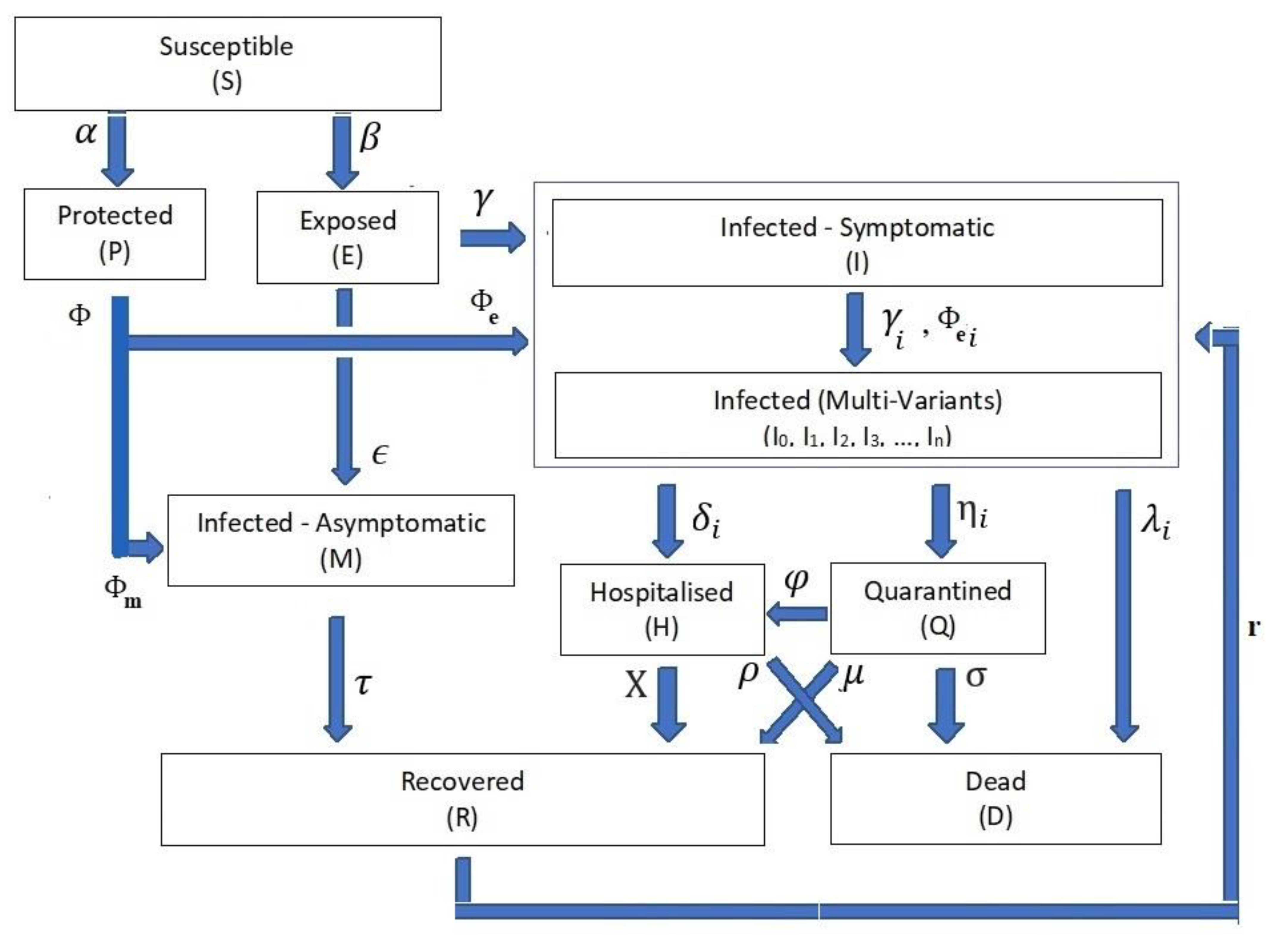
Our new detailed COVID-19 infection model is principally based on the SEIR model [4]. Figure 1 shows the foundation framework of our proposed modelling system. To ease reading the discussions in this paper, we use the following notations:

Figure 1. PCom–SEIR Model Framework with Symptomatic, Asymptomatic, and Multi-Variant Stages.

(1)

The infection stage’s population time-dependent variable is Z(t), where the Z(t) ∈ {S(t), P(t), E(t), I(t), I_i(t), M(t), H(t), Q(t), D(t), R(t)}. Table 1 shows the definitions of these time-dependent variables. For the rest of the paper, we drop the time-independent notation for stage rate variables to ease reading except when necessary.

(2)

The stage parameter variable ψ is defined as ψ ∈ {α, β, ϵ, ϒ, δ_i, η_i, λ_i, μ, χ, σ, ρ, φ}. Table 2 shows the definitions of these parameters as contribution levels from the feeding stage to the target stage. The authors of [3,13] noticed that ψ are time-dependent parameters.

(3)

i ∈ {0, 1, 2, …, n}, where n is defined as the total number of variants, including the mainstream I₀(t).

Table 1. Equation Time-Dependent Variable Descriptions.

	Variable (Z(t))	Description
1	S(t)	The population of the susceptible stage.
2	P(t)	The population of the protected stage.
3	E(t)	The population for the exposed stage.
4	I(t)	The infection population of the symptomatic infection stage.
5	Ii(t), i ∈ {0, 1, 2,…, n}	The population of the ith symptomatic infection variant.
6	M(t)	The population of the asymptomatic infection.
7	Q(t)	The population of the quarantined stage.
8	H(t)	The population of the hospitalisation stage.
9	D(t)	The population of the death stage.
10	N	Country’s population.

Table 1. Equation Time-Dependent Variable Descriptions.

	Variable (Z(t))	Description
1	S(t)	The population of the susceptible stage.
2	P(t)	The population of the protected stage.
3	E(t)	The population for the exposed stage.
4	I(t)	The infection population of the symptomatic infection stage.
5	Ii(t), i ∈ {0, 1, 2,…, n}	The population of the ith symptomatic infection variant.
6	M(t)	The population of the asymptomatic infection.
7	Q(t)	The population of the quarantined stage.
8	H(t)	The population of the hospitalisation stage.
9	D(t)	The population of the death stage.
10	N	Country’s population.

Table 2. Equation Parameter Feed Descriptions.

	Parameter (ψ)	Feeding Parameter
		From Stage	To Stage
1	α	Susceptible (S)	Protected (P)
2	Β		Exposed (E)
3	Φ	Protected (P)
4	Φe	Protected Pe = P ∗ Φe component	Symptomatic infection (I)
5	Φm	Protected Pm = P ∗ Φm component	Asymptomatic infection (M)
6	ϒ	Exposed (E)	Symptomatic infection (I)
7	ϵ		Asymptomatic infection (M)
8	Ii	Symptomatic infection (I)	Symptomatic infection variant i
9	ϒi	Exposed component	Symptomatic infection variant (Ii)
10	Φei	Protected component
11	Δi	Symptomatic variant with (Ii)	Hospitalisation (H)
12	ηi		Quarantine (Q)
13	λi		Death (D)
14	Τ	Asymptomatic (M)	Recovered (R)
15	Χ	Hospitalisation (H)	Recovered (R)
16	Ρ		Death (D)
17	Μ	Quarantine (Q)	Recovered (R)
18	Σ		Death (D)
19	Φ		Hospitalisation (H)
20	ri	Recovered component	Symptomatic infection variant i

Table 2. Equation Parameter Feed Descriptions.

	Parameter (ψ)	Feeding Parameter
		From Stage	To Stage
1	α	Susceptible (S)	Protected (P)
2	Β		Exposed (E)
3	Φ	Protected (P)
4	Φe	Protected Pe = P ∗ Φe component	Symptomatic infection (I)
5	Φm	Protected Pm = P ∗ Φm component	Asymptomatic infection (M)
6	ϒ	Exposed (E)	Symptomatic infection (I)
7	ϵ		Asymptomatic infection (M)
8	Ii	Symptomatic infection (I)	Symptomatic infection variant i
9	ϒi	Exposed component	Symptomatic infection variant (Ii)
10	Φei	Protected component
11	Δi	Symptomatic variant with (Ii)	Hospitalisation (H)
12	ηi		Quarantine (Q)
13	λi		Death (D)
14	Τ	Asymptomatic (M)	Recovered (R)
15	Χ	Hospitalisation (H)	Recovered (R)
16	Ρ		Death (D)
17	Μ	Quarantine (Q)	Recovered (R)
18	Σ		Death (D)
19	Φ		Hospitalisation (H)
20	ri	Recovered component	Symptomatic infection variant i

Based on the above definitions, we can now specify the foundations of the model framework:

 (A) 

Differential Equation System: The relationships from Equations (1)–(10) form the structure of the differential equation set that governs the dynamics of the transitions between the COVID-19 life cycle stages (Figure 1).

$$\frac{dS\left(t\right)}{dt}=-\left(\alpha +\beta \frac{I}{N}\right)S\left(t\right)$$

(1)

$$\frac{dP\left(t\right)}{dt}=\alpha S\left(t\right)-\left( {\Phi }_e+{\Phi }_m \right) P\left(t\right)$$

(2)

where $\left({\Phi }_e+{\Phi }_m\right)$ = $\Phi$

$$\frac{dE\left(t\right)}{dt}=\beta S\left(t\right)\frac{I}{N}-ϵ E\left(t\right)+\gamma E\left(t\right)$$

(3)

$$\frac{dM\left(t\right)}{dt}=ϵ E\left(t\right)-{\Phi }_{m}P\left(t\right)$$

(4)

$$\frac{d{I}_i\left(t\right)}{dt}=-({\delta }_i+{\mathsf{\eta }}_i+{\lambda }_i) I_i\left(t\right)+{\gamma }_{i } E\left(t\right)+{\Phi }_{ei}P\left(t\right)+r_{i}R\left(t\right)$$

(5)

where i ∈ {0, 1, 2, …, n}

$$\frac{dH\left(t\right)}{dt}={\sum }_{i=1}^n{\delta }_i I_i\left(t\right)-\left( \mathsf{{\rm X}}+\rho \right)H\left(t\right)+\phi Q\left(t\right)$$

(6)

$$\frac{dQ\left(t\right)}{dt}={\sum }_{i=1}^n{\mathsf{\eta }}_i{I}_i\left(t\right)-\left(\mu +\mathsf{\sigma }+\phi \right) Q\left(t\right)$$

(7)

$$\frac{dD\left(t\right)}{dt}={\sum }_{i=1}^n{\lambda }_{i } I_i\left(t\right)+\rho H\left(t\right)+\mathsf{\sigma } Q\left(t\right)$$

(8)

$$\frac{dR\left(t\right)}{dt}=\mathrm{X} H\left(t\right)+\mu Q\left(t\right) - r R\left(t\right)$$

(9)

where i ∈ {0, 1, 2, …, n} and n represents the maximum number of variants. The following constraints govern Equation (5):

$$\gamma ={\sum }_1^n{\gamma }_i$$

(10a)

$${\Phi }_e={\displaystyle \sum }_1^n{\Phi }_{ei}$$

(10b)

and

$$I ={\sum }_1^n{I}_i$$

(10c)

Equation (10) must be satisfied at any given point in time over the entire period of observation. The factoring of I(t) in Equation (5) and its impact on Equations (6)–(9) does not mean that we can separately group the equations for each ith variant and then individually find its solution. This statement is based on the fact that the transformation of populations between the proposed stages is not linear; instead, it is an accumulated convolutional relationship [13]. Additionally, the conditions shown in Equation (10) mean that the solutions for each individual stage rate cannot be independently reached. In other words, individual variant optimisation does not guarantee the overall SoDE solution optimisation that constitutes the COVID-19 model. This paper uses the word “model” equivalent to the SoDE “optimum solution”. The word optimum here means that the solution for the {Z(t)} set is not necessarily the best for each individual stage rate but collectively comprises an excellent overall solution.

 (B) 

Stage Population Transition:

Equations (1)–(9) cover the transitions between the listed stage populations in Table 1 and associated transition controlling parameters in Table 2.

 (C) 

Extended Feed Streams:

(C-I) Equations (2), (4) and (5) show that the model accounts for the possibility that some vaccinated (protected (P)) individuals might be infected in the form of symptomatic or asymptomatic infection.

(C-II) Equations (5) and (9) show that the model accounts for the possibility that some recovered (R) individuals might be infected in the form of symptomatic infection.

 (D) 

Infection Categories:

(D-I) The PCom–SEIR framework accounts for the following infection categories: (a) asymptomatic infection M in Equation (4) and (b) symptomatic multi-variant I_i. in Equation (5), which represent a set of equations that describe all I_i variants. In this manner, the new model is not limited to any specific number of variants.

(D-II) Additionally, in Equation (5), the {γ_i}, {Φ_ei}, and {r_i} parameter sets indicate that the individual contribution levels from the exposed stage (E), the protected stage (P), and the recovered (R) stage, respectively, to each ith infection variant (I_i) cannot be guaranteed to be the same.

 (E) 

Health Efforts: It is vitally important to point out that the infection stage’s population Z and the cumulative influencing probability parameter ψ on the infection life cycle govern the transitions’ influx and outflux, as shown in Figure 1. The controlling efforts regulated and imposed by the health authorities are typically the most dominant element within the cumulative parameter due to the state-wide law support. The PCom–SEIR model’s equation parameters map those factors across all stages. Additionally, each of these parameters is a random variable along the time axis. Consequently, the PCom–SEIR model simulates the convoluted impact of the manipulating efforts on each stage population Z. Indeed, this was the basis of the convolution model (CPM) proposed in [13]. Hence, we can write the following:

Z_out(t) = ψ(t)*Z_in(t)

(11)

where * denotes the convolution operation and Z_in(t) and Z_out(t) are the underlying stages of feeding and receiving populations, respectively. Consequently, health authority leaders should be able to drill down each element that influences each Z, providing an opportunity to propose more effective measures.

 (F) 

In and Out Stages’ Population Feeds: The PCom–SEIR model accounts for detailed population feeds for the H, Q, D, and R stages. Such formatting enables the drill-down analysis that many other models lack [2,3,4,5,6,7,8,9,10,11,12,14,15,16,17,49,50].

The feed channels for the H stage, expressed in Equation (6), are:

I.

symptomatic infection variants $\sum _{i=1}^n{\delta }_i\left(t\right) I_i\left(t\right)$;

II.

Q.

The feed channel for the Q stage, expressed in Equation (7), is:

I.

Symptomatic infection variants $\sum _{i=1}^n{\mathsf{\eta }}_i\left(t\right) I_i\left(t\right)$.

The feed channels for the D stage, expressed in Equation (8), are:

I.

symptomatic infection variants $\sum _{i=1}^n{\lambda }_{i }\left(t\right) I_i\left(t\right)$;

II.

H;

III.

Q.

The feed channels for the R stage, expressed in Equation (9), are:

I.

H;

II.

Q;

III.

M.

(G)

Equations’ Constraints:

I.

Equation (10) indicates the governing constraints that ensure the equilibrium between the in and out stage populations within the COVID-19 infection cycle defined from Equations (3)–(9). Equation (10) reflects the fact that all symptomatic infection data I(t) include all variant types without any variant-specific information. This means we could not use published COVID-19 data to verify the derived model. Hence, we needed to use a different approach to validate the derived model, as explained in Section 4.

II.

In Equation (10b), ${\gamma }_i\left(t\right)$ reflects the fact that the effective growth rates I_i(t) of each variant are independent of each other, so there is no guarantee they will have the same rate on a given day. Additionally, this Equation is necessary to ensure the conservation of the total population N. However, there is no well-defined data-based knowledge about the level of impedance of multi-variant infection to vaccination.

4. PCom–SEIR Model Computation

While the PCom–SEIR foundations provide model comprehensiveness, they increase the number of system parameters to 17 + 3 * n (where n is the number of variants) and push the numerical processing time to five hours compared with nine parameters without variants (i.e., n = 1) and two hours of numerical processing [13]. The difference in processing power depends on the Z(t) profile and sizable distracting discontinuity. In our view, the limitations in Equation (10) coupled with the proliferation of equation parameters lead to the narrowing of the solution space, thus reducing error variance and improving the model’s validity. This work used a computing platform based on an Intel i7 CPU @ 2.60 GHz 12 cores with 32 GB of physical memory and a Windows 11 Pro operating system.

To execute the numerical computation to establish a reliable and optimum solution model for the stage rates {Z(t)} in the SoDE (Equations (1)–(9)) and associated conditions in Equation (10) and initial conditions in Table 3, we needed to define the sets of the SoDE use cases. The PCom–SEIR solution describes the rate trends of (a) asymptomatic infection M, (b) interdependent symptomatic infection variants I_i, and (c) the cascading interdependencies between these streams and the Q, H, and R stages. The mapping of the numerical implementation output artefacts to the underlying use cases is exhibited in Table 4. The following are the details of four groups of use cases.

Table 3. Initial Condition Sets.

Initial Condition I
S0	P0	E0	I0	M0	H0	Q0	R0
N	0.1 * N	0.9 * N	I[0]	M[0]	H[0]	Q[0]	R[0]
Initial Condition II
S0	P0	E0	I0	M0	H0	Q0	R0
N	0.7 * N	0.3 * N	1.0	0.0	0.0	0.0	0.0

Table 4. Model Implementation Use Cases.

	Date Range 1			Date Range 2 (Island Range)
560 Points (Days)	23 January 2020, to 5 August 2021			23 April 2020, to 4 November 2021
Initial Conditions (ICs)	I, II	I, II	I, II	I, II	I, II	I, II
Context	Models and Predictions	Parameters	Convergence Ratio	Models and Predictions	Parameters	Convergence Ratio
Canada	Figure 2A(a,b) Figure 2B(a,b)	Figure 2C(a)	Figure 4a	Figure 2A(c,d) Figure 2B(c,d)	Figure 2C(d)	Figure 4a
Saudi Arabia	Figure 3A(a,b) Figure 3B(a,b)	Figure 3C(a)	Figure 4b	Figure 3A(c,d) Figure 3B(c,d)	Figure 3C(d)	Figure 4b

4.1. The Country Use Cases

The COVID-19 data published by the WHO [19,50] for member countries carry the footprint of each country’s health efforts and adopted statistical procedures. Hence, examining the COVID-19 model for more than one country was deemed critical for at least two different use cases: one for Canada and another for Saudi Arabia. The use case for Canada reflects the inherent impact of combining federal and different provincial health controls and district statistical procedures. In contrast, the use case for Saudi Arabia represents one central health system with one set of statistical procedures.

4.2. The Initial Condition Use Cases

Using the two groups of initial conditions (ICs) shown in Table 3 helped verify the model’s responsiveness. Additionally, these ICs assisted our exploration of the impact of vaccination on the model stage profiles. We should point out that the contribution parameters α and β play significant roles in controlling the population feed into the protected (P) and exposed (E) stages, respectively. Consequently, the optimum values of these parameters over the time axis are indirectly determined by the proposed initial conditions, which influence the trend of the solution. The first IC is the actual zero position value of each stage population from the collected data from [19]. The second IC is a hypothetical condition, and its purpose is to introduce a perturbation to the model and observe the model response. This induced response helps detect the solution (model) agility for the underlying scenario.

4.3. Vaccination Representation Use Cases

This work utilised the initial conditions to examine the impact level of vaccination on the model and prediction profile. In Table 3, P₀ for IC-I was set at 10% of N (the entire country’s population), while for IC-II, P₀ was set at 70% of N (the vaccination campaign at the near-completion level). The wide gap of P₀ values was deliberately chosen to enable the scrutinization of the trend of the model profile. The same approach was applied to the infection rate I₀. IC-I was based on actual COVID-19 data, and IC-II was a hypothetical condition used to verify that the solution of the SoDE (i.e., the model) was not the same for all scenarios.

4.4. The Date Range Use Cases

According to Section 2, (1) all COVID-19 variants coexist in addition to the main infection variant, and (2) the variants were not detected until a few months after the emergence of the COVID-19 epidemic. Hence, it is expected that the extent of the date range, in terms of the number of days/points and the range limits, reflects specific behaviour or outline dominance, which would ultimately influence the overall model profile. We devised two date ranges based on this observation to examine the model profile’s changes. In Table 4, these ranges are defined: (1) the first date range spanned from the 0th day to the 560th day, and (2) the second range spans from the 100th day to the 660th day (i.e., island range).

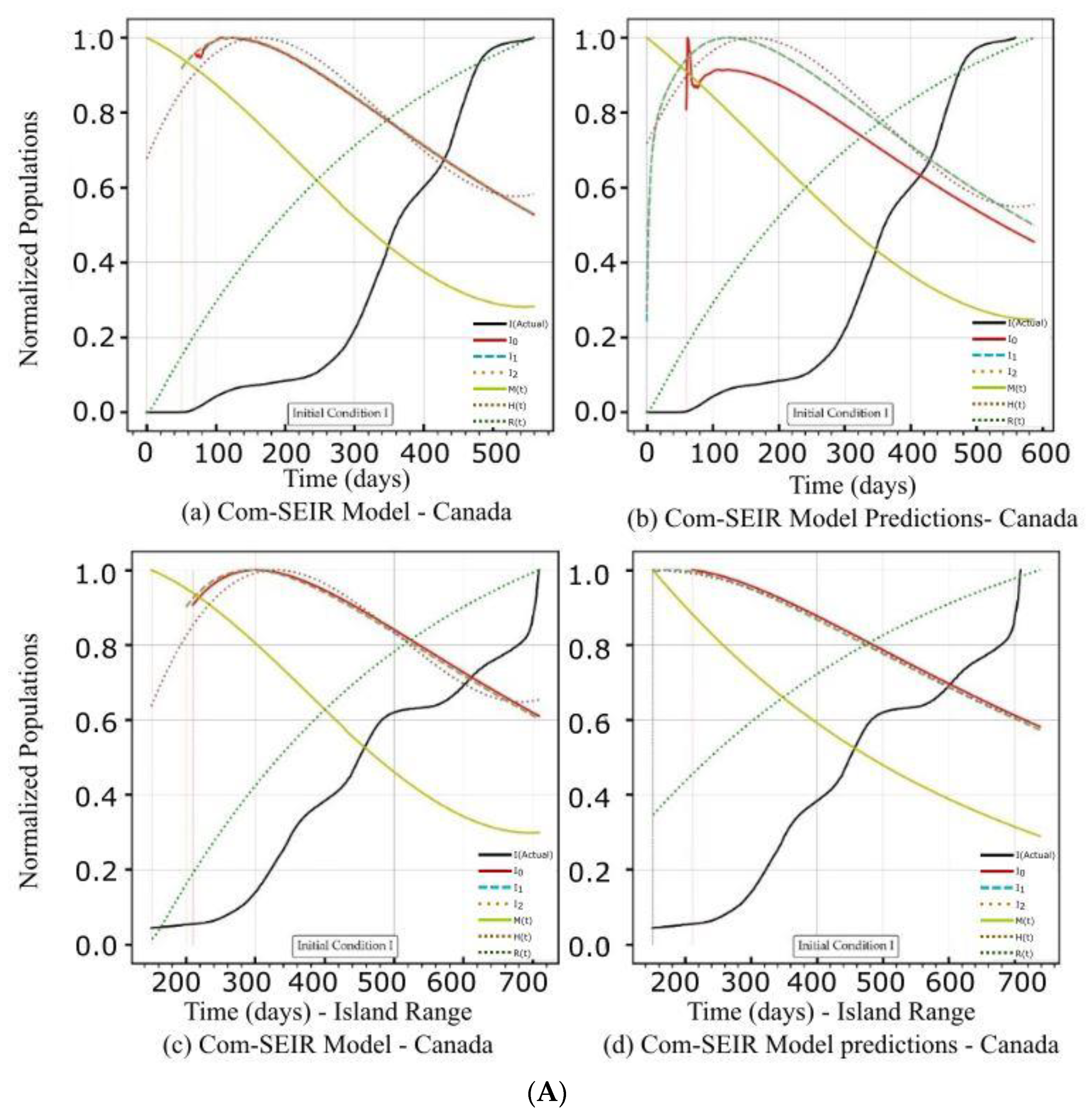
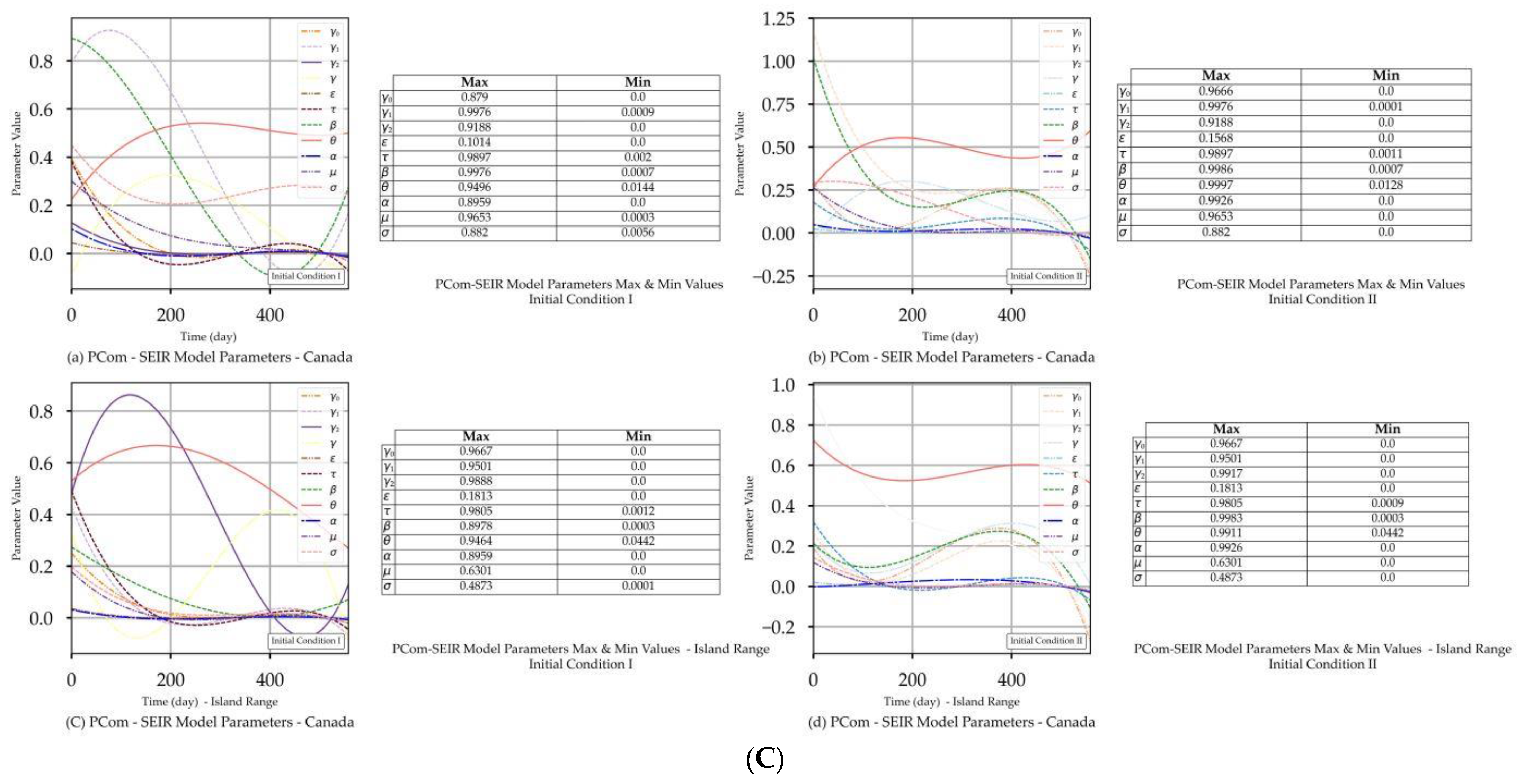
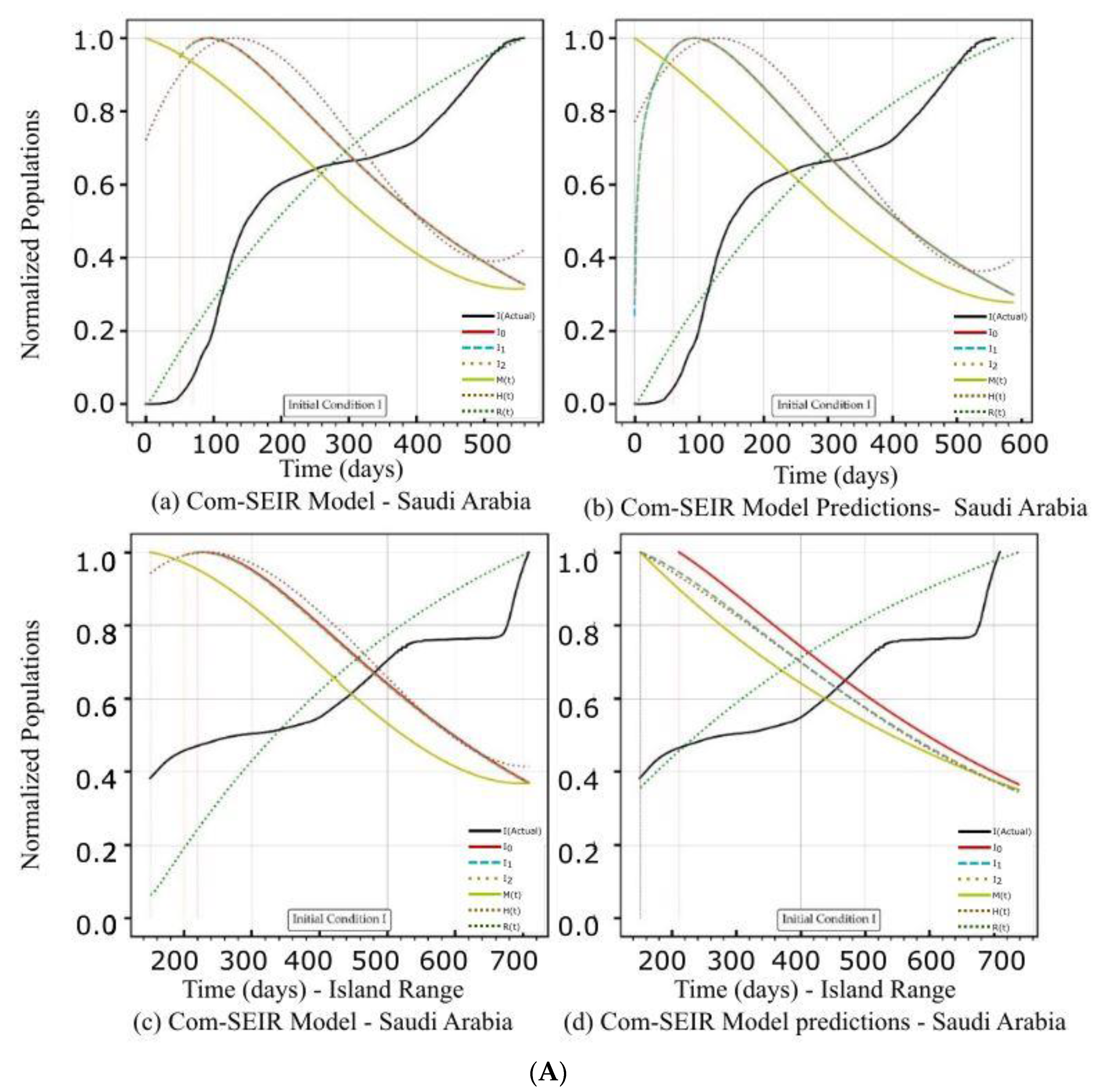
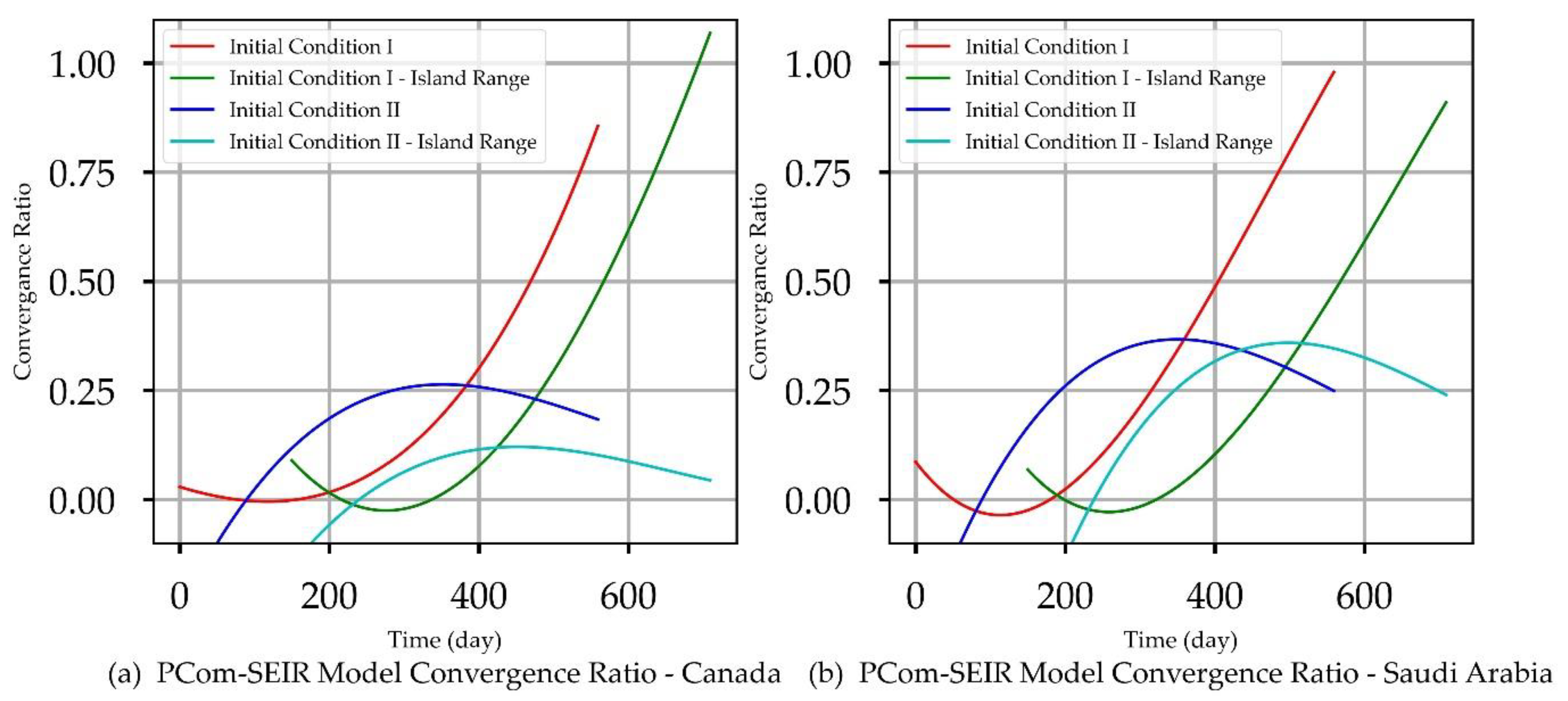
The output of the use cases described the SoDE solution model using 24 artefacts (Figure 2, Figure 3 and Figure 4). These artefacts were organised by country use cases; each group included two sets of ICs and two date ranges that included four diagrams: (I) model stage rates {Z(t)} vs. days, (II) model predictions, (III) equation parameters {ψ} vs. days, and (IV) convergence ratios vs. days. These sets were grouped per each date range use case and for each country use case (Table 4).

Figure 2. (A) PCom–SEIR Model and Prediction Components—Canada. (B) PCom–SEIR Model and Prediction Components—Canada. (C) PCom–SEIR Model Parameters—Canada.

Figure 3. (A) PCom–SEIR Model and Prediction Components—Saudi Arabia. (B) PCom–SEIR Model and Prediction Components—Saudi Arabia. (C) PCom–SEIR Model Parameters—Saudi Arabia.

Figure 4. Solution Convergence Ratios.

4.5. Implementation Steps

As we indicated in our previous work [13], to determine the optima in a 2D space, most classical optimisation strategies rely on evaluating the first derivative Z′(t) and the second derivative Z″(t). There is no certainty that the first or second derivative exists, so finding the optimal solution for many rough and discontinuous surfaces is risky. Many numerical computation libraries start by smoothing the input data and then finding the solution in response to such a challenge. This approach has an inherent risk of increasing the RMSE for most data grid points due to the expansion of the solution surface, and it might mask some behaviours of interest. As a result, one must employ a derivative-free optimisation strategy such as an intelligent search problem [51]. For a core optimisation problem, one or more computational agents are used to find the optima in a real-value search space with its embedded set of initial conditions [19]. The particle swarm optimisation (PSO) approach [49] and the differential evolution (DE) method [51] are two of the most prominent algorithms. The DE method is a type of differential operator that may be readily invoked and implemented by adjusting model parameters [19]. In this study, the Python DE library [52] provided the opportunity to collect the optimum equation parameters, listed in Table 2, at each solution point Z(t) via a user-defined callback function of a defined signature. This callback signature included two global static arrays. The first array was used to calculate the 17 + 3 parameters, where each was associated with a corresponding solution point Z(t). The second array was used to calculate the solution convergence ratio at each solution point Z(t). The Python DE library’s main optimisation call takes a pointer to the callback function as one of its call attributes, and this callback function then populates the global/static m-dimensional array and one-dimensional convergence array, where m = 20. Here, the DE library optimisation call also let us choose one of three optimum search algorithms; we chose “best1bin”.

To ensure the restriction of the optimum solution surface to minimise the RMSE values for each parameter, we had to define the relevant value limitations in Equations (1)–(9) to guarantee the good conservation of the overall country’s population N and to satisfy the definition of the parameters’ weighting role. To deploy such a mechanism into the DE optimisation Python call, we introduced 0.0 to 1.0 limits to each parameter. We used these parameters’ limits in an array and passed them to the DE call as one of its parameters. The DE library used these limits as guidance rather than imposed limits. The DE package has a built-in curve smoothing at the final stage of its computation, which usually uses the entire length of the data grid as a smoothing window. As a result of this intrinsic feature, a model profile has one peak and lacks incremental behaviour [13].

5. Results and Discussion

The mappings of Canadian and Saudi Arabian use cases to the results’ artefacts are illustrated in Table 4. Section 5.1 and Section 5.2 exhibit and review the results for Date Range 1 and Date Range 2 (Table 4) for Canada and Saudi Arabia, respectively, for each initial condition in Table 3. These sections also include the model validity and reliability indicators. The issue of solution discontinuity and convergence is assessed for all use cases concerning Figure 4.

5.1. PCom–SEIR Model and 30-Day Prediction for Canada

The artefacts in Figure 2A(a,b),B(a,b) show the convergence weakness of the solution over the first 50 points. This means that the Python DE package required a finer mesh (i.e., a quarter or half-day point set) of data to build up the search intelligence to find a suitable solution point. In other words, the starting points of the COVID-19 data grid truly had no first and second derivatives. The root causes of such “dirty” data were: (1) the data needed to be collected more than once per day, and (2) the data were not statistically appropriately collected. This statement is based on the fact that the Canadian data had significantly more convergence issues (Figure 2A(a,b),B(c,d)) than the Saudi Arabian data (Figure 3A(a,b)). The discontinuity issue manifested the low convergence ratio shown in Figure 4a.

Figure 2C and Figure 3C show that extracted equation parameters {ψ} (see Section 4.5) had a time-dependency. The figures also show the minimum and maximum values of the corresponding {ψ} set members.

The rates of the asymptomatic infection M, hospitalised H, and recovered R exhibited different profiles for both sets of initial conditions and over the date ranges. Here, we focus on the symptomatic infection variants’ {I_i} rate curves’ behaviour as they showed broad changes that are reviewed in Table 5 and Table 6. Comparing the decline slope in Table 5 and Table 6 and observing the diagrams in Figure 2A(a–d) for IC-I and Figure 2B(a–d) for IC-II reveals that induced protection (P₀ = 70%) in IC-II produced the expected increase in the decline slope of the symptomatic infection variants {I_i}.

Table 5. Summary Discussion for Initial Conditions I—Canada.

	Date Range 1 (Start Date: 0 Days).		Date Range 2 (Start Date: 100 Days).
Figure	Model—Figure 2A(a)	Prediction—Figure 2A(b)	Model—Figure 2A(c)	Prediction—Figure 2A(d)
Curve discontinuity	Not stable over the first 50+ days.		The {Ii} curves showed an improvement, but we still needed to truncate the curve’s start by 20 points.	The prediction curves for {I1, I2} did not show discontinuity, but I0 (main stream) did.
Peak position	The first peaks located before the 100 days were due to solution discontinuity. The peak on the 120th day was within the range of the actual stable solution.		The curves for {Ii} had nearly the same peak on the 200th day after the start date.	The {Ii} curves shared the same peak on the 110th day after the start date.
Curve profiles	The {Ii} curves showed the same profile with a limited plateau.	The {Ii} curves showed different individual profiles but all had small plateaus.	The {Ii} curves showed the same profile with a noticeable plateau.	The {Ii} curves showed the same profile but differed from the models.
Decline rate	The predicted declines of the infection growth rate were relatively slower than those of the model.		The predicted infection growth rate declines were slower than those of the models.
Decline slope	2.15/4	2.0/4	2.2/4	1.9/4

Table 6. Summary Discussion for Initial Conditions II—Canada.

	Date Range 1 (Start Date: 0 Days).		Date Range 2 (Start Date: 100 Days).
Figure	Model—Figure 2B(a)	Prediction—Figure 2B(b)	Model—Figure 2B(c)	Prediction—Figure 2B(d)
Curve discontinuity	Relatively stable over the first 50 days.		The {I1, I2} curves did not show a realistic solution, but I0 (main stream) did.
Peak position	The peak appeared on the 110th day.	The peak appeared on the 100th day.	The I0 curve peaked at the 150th day (i.e., 250th day) after the start date.	The I0 curve showed no peak.
Curve profiles	The {Ii} curves showed the same profile with a limited plateau.	The {Ii} curves showed different individual profiles with a limited plateau.	The I0 curve showed nearly the exact profile of Date Range 1 with a finite plateau.	The I0 curve showed a different profile than the model without a plateau.
Decline rate	The predicted infection growth decline was at nearly the same rate as that of the model. However, it showed a steeper decline than that of IC-I.		The predicted infection growth decline rate was slower than that of the model.
Decline slope	2.5/4	2.5/4	2.4/4	2.1/4

5.1.1. Initial Conditions I—Canada

Initial Conditions I was based on actual COVID-19 data. It assumed the zero positions of the stage growth rates {Z(t)} (Table 3). It is vitally important to mention that the solutions in Figure 2A(a) and the corresponding 30-day prediction in Figure 2A(b) were unstable over the first 50+ days. This discontinuity caused the appearance of early peaks. The peaks for the actual solutions (for the model prediction curves) appeared on the 120th day. Figure 4a shows that the solution convergence ratio was very low and even negative over some early points. Over these early points, the DE algorithm needed help establishing a safe solution. To partially overcome this challenge, we truncated the beginning of the curve. We utilised external curve smoothing with a small smoothing window to overcome this aberration and preserve the actual curve behaviour. The observed discontinuity was much less in the island range.

5.1.2. Initial Conditions II—Canada

In this section, we discuss the impact of IC-II on the model and prediction curves over the two date ranges (Table 4). While IC-I was based on actual values, IC-II was an artificial initial condition that was mainly used to examine the model behaviour under induced conditions (Table 3). In this manner, we tested the sensitivity of the solution beyond its intended data scope to show the validity of the model framework approach. The model and prediction curves’ steeper decline shown in Figure 2B(a,c) and in Figure 2B(b,d), respectively, was induced by the 70% P₀ in IC-II. In other words, vaccination slowed down the infection growth rate. This observation is one of the model formulation’s validation indicators. Additionally, Figure 2B(c,d) show significant discontinuity issues for the {I₁, I₂} solutions. This discontinuity reflects the low convergence ratio shown in Figure 4a. We can observe that the solution convergence ratio was more than 0.25 for IC-II. This is a good validity and reliability indicator for the PCom–SEIR formulation; different initial conditions led to different solution spaces with different levels of point convergence.

5.2. PCom–SEIR Model and 30-Day Prediction for Saudi Arabia

Reviewing the artefacts in Figure 3A(a,b),B(a–d) and Figure 4b indicates that the solution convergence issue was mild, as shown in Figure 2A(a,b),B(a–d) and Figure 4a over the first 50 points. This could be attributed to the fact that the collected COVID-19 data for Saudi Arabia were more statistically coherent than those for Canada. The better data quality could be attributed to Saudi Arabia’s unified health controls, as Canada’s are a mixture of federal and several local health control systems.

Figure 4b indicates that the solution’s convergence was weak over the first 50 points but less severe than that of Range 1. Comparing the PCom–SEIR model’s curves for {I_i} in Figure 3A(c,d),B(c,d) (for Range 2) with the corresponding curves in Figure 3A(a,b),B(a,b) reveals that the model’s curves showed a sharper decline over Range 2. This result indicates that Range 2 had more health controls (i.e., more vaccinations) than Range 1. This is significant evidence that indicates the high reliability of the new PCom–SEIR model. Section 5.2.1 and Section 5.2.2 provide detailed discussions in this regard.

The rates for asymptomatic infection M, hospitalised H, and recovered R showed different profiles for both sets of the initial conditions over both date ranges. In this section, we focus on the symptomatic infection variant {I_i} rate curves’ behaviour, as they showed broad changes that are summarised in Table 7 and Table 8. Comparing the decline slopes in Table 7 and Table 8 and observing the diagrams in Figure 3A(a–d) for IC-I and Figure 3B(a–d) for IC-II reveals that the induced protection (P₀ = 70%) in IC-II produced the expected increase in the decline slope of the symptomatic infection variants {I_i}.

Table 7. Summary Discussion for Initial Conditions I—Saudi Arabia.

	Date Range 1 (Start Date: 0 Days).		Date Range 2 (Start Date: 100 Days).
Figure	Model—Figure 3A(a)	Prediction—Figure 3A(b)	Model—Figure 3A(c)	Prediction—Figure 3A(d)
Curve discontinuity	The {Ii} curves showed an improvement, but we still needed to truncate the curve’s start by 50 points.	The {Ii} curves showed good improvement without the need to truncate the curve’s start.	The {Ii} curves showed an improvement, but we still needed to truncate the curve’s start by 50 points.	The prediction curves for {Ii} did not show a discontinuity.
Peak position	The peaks appeared on the 110th day.	The peaks appeared on the 90th day.	The curves for {Ii} had nearly the same peak on the 120th day after the start date.	The {I1, I2} curves shared the same peak on the 30th day after the start date. I0 showed no peak.
Curve profiles	The {Ii} curves showed the same profile with a noticeable plateau.	The {Ii} curves showed the same profile with a noticeable plateau. The prediction profile was different from the model curve profiles.	The {Ii} curves showed the same profile with a small plateau.	The {I1, I2} curves showed the same profile, while I0 showed a distinct profile. This indicates that there was a different level of infection dominance.
Decline rate	The predicted and model infection growth decline rates were the same.		The predicted infection growth decline rates were slower than those of the model.
Decline slope	3.1/4	3.1/4	3.1/4	2.2, 2.2, 2.5/4

Table 8. Summary Discussion for Initial Conditions II—Saudi Arabia.

	Date Range 1 (Start Date: 0 Days).		Date Range 2 (Start Date: 100 Days).
Figure	Model—Figure 3B(a)	Prediction—Figure 3B(b)	Model—Figure 3B(c)	Prediction—Figure 3B(d)
Curve discontinuity	The {Ii} curves showed an improvement, but we still needed to truncate the curve’s start by 50 points.		The {Ii} curves showed improvement with the need to truncate the curve’s start.	The {Ii} curves showed an improvement, but we still needed to truncate the curve’s start by 50 points.
Peak position	The peaks appeared on the 100th day.		The peaks appeared on the 95th day.	The {I1, I2} curves had different maxima, with the same peak on the 120th day after the start date.
Curve profiles	The {Ii} curves showed the same profile with a noticeable plateau.	The {Ii} curves showed the same profile with a noticeable plateau. The prediction profile was different from the model curve profiles.	The {Ii} curves showed practically the same profile without a plateau.	The {I1, I2} curves showed the same profile, while I0 showed a distinct profile. This indicates that there was a different level of infection dominance.
Decline rate	The predicted infection growth decline rates were slightly slower than those of the model.		The rate of infection growth decline was relatively slower than that of the model.
Decline slope	3.3/4	3.3/4	3.3/4	3.2, 3.3, 3.4/4

5.2.1. Initial Conditions I—Saudi Arabia

The model’s curves for Saudi Arabia are shown in Figure 3A(a,b) under IC-I. These curves had different profiles than those in Figure 3A(c,d). Since the convergence was not severe in this use case, no external curve smoothing was utilised. As in Figure 2A(c,d) and Figure 3A(c,d) shows that the equation parameters {ψ} had time-dependency. In Figure 3A(a) for IC-I, the three symptomatic infection variants {I_i}, where i ∈ {0, 1, 2}, exhibit their peaks at the same point and the same curve profile. In Figure 3B(b) for IC-II, the I₀ curve shows an early narrow peak and sharp decline, while I₁ and I₂ show different profiles, which could indicate instability in the solution curves. In Figure 3A(a,b), the M curves for asymptomatic infection for IC-I and IC-II display different profiles but share the same declining trends at the end of the date period. Additionally, Figure 3A(b) shows that the induced 70% protection bias embedded in IC-II (which represents the vaccination) clearly impacted I₀ because it had an earlier peak and a steeper decline than I₀ for IC-I in Figure 3A(a). The profiles of symptomatic infection variants I₁ and I₂ shown in Figure 3A(b) exhibit different behaviours than those in Figure 3A(a) for IC-I, which is attributed to a different level of dominance for I₁ and I₂ in Date Range 2 than in Date Range 1.

5.2.2. Initial Conditions II—Saudi Arabia

In this section, we discuss the impact of IC-II on the model and 30-day prediction curves over the two date ranges (Table 4). The sensitivity of the solution beyond its intended data space is explored to show the validity of the model framework approach. The model and prediction curves’ steeper decline shown in Figure 3B(a,c) and in Figure 3B(b,d), respectively, was induced by the 70% P₀ in IC-II. In other words, vaccination slowed down the infection growth rate. This observation is one of the model formulation’s validation indicators. The level of discontinuity for Saudi Arabia was reflected by the better low convergence ratio shown in Figure 4b. This result is a good validity and reliability indicator for the PCom–SEIR formulation; different data sources led to different solution spaces with different levels of convergence.

6. Conclusions

The formulation of the published SEIR models was based on a framework that includes the typical COVID-19 transition stages and their direct feeding streams. However, such foundations do not include indirect feeding streams that influence the infection stage. Additionally, these models do not consider multiple variants for symptomatic infection. Such exclusions resulted in a skewed model of the published data. These models are still valid and logical, though strictly under their assumptions. Additionally, the model validation could be mapped 1:1 to the published data schema.

In reality, published COVID-19 data mask indirect feeding streams and multi-variant infections. The decomposition mask is due to the limited testing capacity of health authorities. Our new, comprehensive polymorphic SEIR model (PCom–SEIR) considers indirect feeding streams and multi-variant infections. This means that the PCom–SEIR framework data object instance inherits a schema as a concrete data class from the published data. In addition to the inherited data schema, the PCom–SEIR data class includes the new model schema specifics (i.e., extra feeding streams and multi-variant infections). Consequently, we were not able to 1:1 map the new data model with the published data schema. Hence, we were not able to use COVID-19 data for model validation. To facilitate the validation of the new model, we had to deploy an X-ray examination by designing a set of use cases (scenarios) to cover a broad scope of model examinations. Additionally, we needed to verify the generality of the PCom–SEIR model. Such a task is not required for other models because they are specific to the minimum of feeding streams and do not consider multi-variant infections.

The new PCom–SEIR model validation and reliability examination steps were based on: (I) devising a diverse set of use cases for (a) two sets of initial conditions, (b) two sets of the data range, and (c) two different health authorities (Canada and Saudi Arabia); (II) generality testing by reducing the scope of PCom–SEIR to a typical, simple SEIR model.

6.1. Validity and Reliability Use Cases

The results shown in Figure 2, Figure 3 and Figure 4 indicate the reliability of the new PCom–SEIR model in terms of the prominent rate model trends for {I_i}, M, Q, and R over a broad scope of use cases involving (a) two different sets of initial conditions, (b) different date range sets with different events’ dominance, and (c) two countries’ COVID-19 data under two different health system controls. The summary of the models’ behaviours in Table 5 and Table 6 for Canada and Table 7 and Table 8 for Saudi Arabia exhibits many indicators that the model is valid and reliable. These indicators support the finding that the new PCom–SEIR model had no fixed profile for all scenarios. This observation is a good indicator of the model’s credibility.

6.2. Model Generality

The SoDE (Equations (1)–(10)) represents the general and comprehensive model format. The new PCom–SEIR model could also be validated by reducing its SoDE to a particular case by eliminating some of the stage feed elements (Figure 1 and Table 2), namely: (I) the 3rd, 4th, 5th, and the 10th streams, which controlled the direct feed from the protected stage (P) to the symptomatic infection stage (I); (II) the 14th stream, which controlled the feed from the asymptomatic (M) feed to the recorded stage (R); and (III) the 20th stream, which controlled the feed from the recovered stage (R) to the symptomatic infection stage (I). Such simplifications led to the production of the models shown in Figure 5A for Canada and Figure 5B for Saudi Arabia. This model’s simplification showed that (I) the extended stage feeds had a considerable impact on the general profiles of the model’s curve, and (II) reducing the number of parameters helped improve the solution stability over the initial period.

Figure 5. (A) Simplified PCom–SEIR Model Components—Canada. (B) Simplified PCom–SEIR Model Components—Saudi Arabia.

The main conclusion of Section 6.1 and Section 6.2 is that the new PCom–SEIR model is polymorphic and reusable across many scenarios.

6.3. Future Work—Hybrid Approach

We are going to adopt a hybrid approach to deduce the profiles for symptomatic infection variants {I_i}. The first step in this approach is to collapse the set of Equation (5) for {I_i} into a unified equation for the symptomatic infection I. The methodology we are now researching will be used to determine the set {I_i} outside the model’s equations. Then, we will analyse the computed unified I into its assumed infection variants {I_i} using the Gaussian Mixture Model (GMM) algorithm [53,54], which is a typical machine learning algorithm for clustering. This hybrid approach will be the topic of our subsequent publication.

References

- Lv, L.; Li, G.; Chen, J.; Liang, X.; Li, Y. Comparative genomic analysis revealed specific mutation pattern between human coronavirus SARS-CoV-2 and Bat-SARSr-CoV RaTG13. BioRxiv 2020. [Google Scholar] [CrossRef]
- Balabdaoui, F.; Mohr, D. Age-stratified discrete compartment model of the COVID-19 epidemic with application to Switzerland. Sci. Rep. 2020, 10, 21306. [Google Scholar] [CrossRef] [PubMed]
- Giordano, G.; Blanchini, F.; Bruno, R.; Colaneri, P.; Di Filippo, A.; Di Matteo, A.; Colaneri, M. Modelling the COVID-19 epidemic and implementation of population-wide interventions in Italy. Nat. Med. 2020, 26, 855–860. [Google Scholar] [CrossRef]
- Godio, A.; Pace, F.; Vergnano, A. SEIR Modeling of the Italian Epidemic of SARS-CoV-2 Using Computational Swarm Intelligence. Int. J. Environ. Res. Public Health 2020, 17, 3535. [Google Scholar] [CrossRef] [PubMed]
- Shaikh, A.S.; Shaikh, I.N.; Nisar, K.S. A Mathematical Model of COVID-19 Using Fractional Derivative: Outbreak in India with Dynamics of Transmission and Control. Adv. Differ. Equ. 2020, 2020, 373. [Google Scholar] [CrossRef]
- Lin, Q.; Zhao, S.; Gao, D.; Lou, Y.; Yang, S.; Musa, S.S.; Wang, M.H.; Cai, Y.; Wang, W.; Yang, L.; et al. A conceptual model for the coronavirus disease 2019 (COVID-19) outbreak in Wuhan, China with individual reaction and governmental action. Int. J. Infect. Dis. 2020, 93, 211–216. [Google Scholar] [CrossRef]
- Roques, L.; Klein, E.K.; Papaix, J.; Sar, A.; Soubeyrand, S. Using Early Data to Estimate the Actual Infection Fatality Ratio from COVID-19 in France. Biology 2020, 9, 97. [Google Scholar] [CrossRef]
- Bakhta, A.; Boiveau, T.; Maday, Y.; Mula, O. Epidemiological Forecasting with Model Reduction of Compartmental Models. Application to the COVID-19 Pandemic. Biology 2021, 10, 22. [Google Scholar] [CrossRef]
- Mokhtari, A.; Mineo, C.; Kriseman, J.; Kremer, P.; Neal, L.; Larson, J. A multi method approach to modeling COVID 19 disease dynamics in the United States. Sci. Rep. 2021, 11, 12426. [Google Scholar] [CrossRef]
- Xie, G. A novel Monte Carlo simulation procedure for modelling COVID-19 spread over time. Sci. Rep. 2020, 10, 13120. [Google Scholar] [CrossRef]
- Sartorius, B.; Lawson, A.B.; Pullan, R.L. Modelling and predicting the spatiotemporal spread of COVID-19, associated deaths and impact of key risk factors in England. Sci. Rep. 2021, 11, 5378. [Google Scholar] [CrossRef]
- Mishra, S.; Scott, J.A.; Laydon, D.J.; Flaxman, S.; Gandy, A.; Mellan, T.A.; Unwin, H.J.T.; Vollmer, M.; Coupland, H.; Ratmann, O.; et al. Comparing the responses of the UK, Sweden, and Denmark to COVID 19 using counterfactual modelling. Sci. Rep. 2021, 11, 16342. [Google Scholar] [CrossRef] [PubMed]
- Al-Hadeethi, Y.; Ramley, I.F.E.; Sayyed, M.I. Convolution model for COVID-19 rate predictions and health effort levels computation for Saudi Arabia, France, and Canada. Sci. Rep. 2021, 11, 22664. [Google Scholar] [CrossRef] [PubMed]
- Bastos, S.B.; Cajueiro, D.O. Modeling and forecasting the early evolution of the COVID-19 pandemic in Brazil. Sci. Rep. 2020, 10, 19457. [Google Scholar] [CrossRef]
- Liu, M.; Thomadsen, R.; Yao, S. Forecasting the spread of COVID-19 under different reopening strategies. Sci. Rep. 2020, 10, 20367. [Google Scholar] [CrossRef] [PubMed]
- Zhang, Y.; You, C.; Cai, Z.; Sun, J.; Hu, W.; Zhou, X.H. Prediction of the COVID-19 outbreak in China based on a new stochastic dynamic model. Sci. Rep. 2020, 10, 21522. [Google Scholar] [CrossRef]
- Ma, R.; Zheng, X.; Wang, P.; Liu, H.; Zhang, C. The prediction and analysis of COVID-19 epidemic trend by combining LSTM and Markov method. Sci. Rep. 2021, 11, 17421. [Google Scholar] [CrossRef]
- Oraby, T.; Tyshenko, M.G.; Maldonado, J.C.; Vatcheva, K.; Elsaadany, S.; Alali, W.Q.; Longenecker, J.C.; Al-Zoughool, M. Modeling the effect of lockdown timing as a COVID-19 control measure in countries with differing social contacts. Sci. Rep. 2021, 11, 3354. [Google Scholar] [CrossRef]
- GitHub. Available online: https://raw.githubusercontent.com/datasets/covid-19/master/data/countries-aggregated.csv (accessed on 22 September 2021).
- WHO. Available online: https://www.who.int/news-room/fact-sheets/detail/middle-east-respiratory-syndrome-coronavirus-(mers-cov) (accessed on 28 October 2021).
- Gorbalenya, A.E.; Baker, S.C.; Baric, R.S.; de Groot, R.J.; Drosten, C.; Gulyaeva, A.A.; Haagmans, B.L.; Lauber, C.; Leontovich, A.M.; Neuman, B.W.; et al. The species Severe acute respiratory syndrome-related coronavirus: Classifying 2019-nCoV and naming it SARS-CoV-2. Nat. Microbiol. 2020, 5, 536. [Google Scholar]
- Na, W.; Moon, H.; Song, D. A comprehensive review of SARS-CoV-2 genetic mutations and lessons from animal coronavirus recombination in one health perspective. J. Microbiol. 2021, 59, 332–340. [Google Scholar] [CrossRef]
- Ahn, D.G.; Shin, H.J.; Kim, M.H.; Lee, S.; Kim, H.S.; Myoung, J.; Kim, B.T.; Kim, S.J. Current status of epidemiology, diagnosis, therapeutics, and vaccines for novel coronavirus disease 2019 (COVID-19). J. Microbiol. Biotechnol. 2020, 30, 313–324. [Google Scholar] [CrossRef]
- Tu, Y.F.; Chien, C.S.; Yarmishyn, A.A.; Lin, Y.Y.; Luo, Y.H.; Lin, Y.T.; Lai, W.Y.; Yang, D.M.; Chou, S.J.; Yang, Y.P.; et al. A review of SARS-CoV-2 and the ongoing clinical trials. Int. J. Mol. Sci. 2020, 21, 2657. [Google Scholar] [CrossRef]
- Wu, Z.; McGoogan, J.M. Characteristics of and important lessons from the coronavirus disease 2019 (COVID-19) outbreak in China: Summary of a report of 72 314 cases from the Chinese Center for Disease Control and Prevention. JAMA 2020, 323, 1239–1242. [Google Scholar] [CrossRef]
- Huang, N.E.; Qiao, F. A data-driven time-dependent transmission rate for tracking an epidemic: A case study of 2019-nCoV. Sci. Bull. 2020, 65, 425. [Google Scholar] [CrossRef] [PubMed]
- Available online: https://www.worldometers.info/coronavirus/#countries (accessed on 5 October 2021).
- Available online: https://www.who.int/en/activities/tracking-SARS-CoV-2-variants (accessed on 2 October 2021).
- Shen, X.; Tang, H.; McDanal, C.; Wagh, K.; Fischer, W.; Theiler, J.; Yoon, H.; Li, D.; Haynes, B.F.; Sanders, K.O.; et al. SARS-CoV-2 variant B. 1.1. 7 is susceptible to neutralising antibodies elicited by ancestral spike vaccines. Cell Host Microbe 2021, 29, 529–539. [Google Scholar] [CrossRef]
- Altmann, D.M.; Boyton, R.J.; Beale, R. Immunity to SARS-CoV-2 variants of concern. Science 2021, 371, 1103–1104. [Google Scholar] [CrossRef] [PubMed]
- Rees-Spear, C.; Muir, L.; Griffith, S.A.; Heaney, J.; Aldon, Y.; Snitselaar, J.L.; Thomas, P.; Graham, C.; Seow, J.; Lee, N.; et al. The effect of spike mutations on SARS-CoV-2 neutralisation. Cell Rep. 2021, 34, 108890. [Google Scholar] [CrossRef] [PubMed]
- Hu, J.; Peng, P.; Wang, K.; Fang, L.; Luo, F.Y.; Jin, A.S.; Liu, B.Z.; Tang, N.; Huang, A.L. Emerging SARS-CoV-2 variants reduce neutralisation sensitivity to convalescent sera and monoclonal antibodies. Cell. Mol. Immunol. 2021, 18, 1061–1063. [Google Scholar] [CrossRef]
- Wang, P.; Nair, M.S.; Liu, L.; Iketani, S.; Luo, Y.; Guo, Y.; Wang, M.; Yu, J.; Zhang, B.; Kwong, P.D.; et al. Antibody resistance of SARS-CoV-2 variants B.1.351 and B.1.1.7. Nature 2021, 593, 130–135. [Google Scholar] [CrossRef] [PubMed]
- Moyo-Gwete, T.; Madzivhandila, M.; Makhado, Z.; Ayres, F.; Mhlanga, D.; Oosthuysen, B.; Lambson, B.E.; Kgagudi, P.; Tegally, H.; Iranzadeh, A.; et al. SARS-CoV-2 501Y. V2 (B. 1.351) elicits cross-reactive neutralising antibodies. bioRxiv 2021. preprint. [Google Scholar]
- Koyama, T.; Platt, D.; Parida, L. Variant analysis of SARS-CoV-2 genomes. Bull. World Health Organ. 2020, 98, 495. [Google Scholar] [CrossRef]
- Slavov, S.N.; Patané, J.S.; Bezerra, R.D.S.; Giovanetti, M.; Fonseca, V.; Martins, A.J.; Viala, V.L.; Rodrigues, E.S.; Santos, E.V.; Barros, C.R.; et al. Genomic monitoring unveil the early detection of the SARS-CoV-2 B. 1.351 lineage (20H/501Y. V2) in Brazil. J. Med. Virol. 2021, 93, 6782–6787. [Google Scholar] [CrossRef] [PubMed]
- Shen, X.; Tang, H.; Pajon, R.; Smith, G.; Glenn, G.M.; Shi, W.; Korber, B.; Montefiori, D.C. Neutralisation of SARS-CoV-2 Variants B.1.429 and B.1.351. N. Engl. J. Med. 2021, 384, 2352–2354. [Google Scholar] [CrossRef]
- Singh, J.; Samal, J.; Kumar, V.; Sharma, J.; Agrawal, U.; Ehtesham, N.Z.; Sundar, D.; Rahman, S.A.; Hira, S.; Hasnain, S.E. Structure-Function Analyses of New SARS-CoV-2 Variants B.1.1.7, B.1.351 and B.1.1.28.1: Clinical, Diagnostic, Therapeutic and Public Health Implications. Viruses 2021, 13, 439. [Google Scholar] [CrossRef] [PubMed]
- Gupta, R.K. Will SARS-CoV-2 variants of concern affect the promise of vaccines? Nat. Rev. Immunol. 2021, 21, 340–341. [Google Scholar] [CrossRef] [PubMed]
- Focosi, D.; Maggi, F. Neutralising antibody escape of SARS-CoV-2 spike protein: Risk assessment for antibody-based COVID-19 therapeutics and vaccines. Rev. Med. Virol. 2021, 31, e2231. [Google Scholar] [CrossRef] [PubMed]
- Fontanet, B.; Autran, B.; Lina, M.P.; Kieny, S.S.; Karim, A.; Sridhar, D. SARS-CoV-2 variants and ending the COVID-19 pandemic. Lancet 2021, 397, 952–954. [Google Scholar] [CrossRef] [PubMed]
- Campbell, F.; Archer, B.; Laurenson-Schafer, H.; Jinnai, Y.; Konings, F.; Batra, N.; Pavlin, B.; Vandemaele, K.; Van Kerkhove, M.D.; Jombart, T.; et al. Increased transmissibility and global spread of SARS-CoV-2 variants of concern as at June 2021. Eurosurveillance 2021, 26, 2100509. [Google Scholar] [CrossRef] [PubMed]
- Mohammadi, M.; Shayestehpour, M.; Mirzaei, H. The impact of spike mutated variants of SARS-CoV2 [Alpha, Beta, Gamma, Delta, and Lambda] on the efficacy of subunit recombinant vaccines. Braz. J. Infect. Dis. 2021, 25, 101606. [Google Scholar] [CrossRef]
- Hajj-Hassan, H.; Hamze, K.; Sater, F.A.; Kizilbash, N.; Khachfe, H.M. Probing the Increased Virulence of Severe Acute Respiratory Syndrome Coronavirus 2 B.1.617 (Indian Variant) From Predicted Spike Protein Structure. Cureus 2021, 13, e16905. [Google Scholar] [CrossRef]
- Romero, P.E.; Dávila-Barclay, A.; Salvatierra, G.; González, L.; Cuicapuza, D.; Solís, L.; Marcos-Carbajal, P.; Huancachoque, J.; Maturrano, L.; Tsukayama, P. The emergence of SARS-CoV-2 variant lambda (C. 37) in South America. Microbiol. Spectr. 2021, 9, e00789-21. [Google Scholar] [CrossRef]
- Tada, T.; Zhou, H.; Dcosta, B.M.; Samanovic, M.I.; Mulligan, M.J.; Landau, N.R. SARS-CoV-2 lambda variant remains susceptible to neutralisation by mRNA vaccine-elicited antibodies and convalescent serum. bioRxiv 2021. preprint. [Google Scholar]
- Acevedo, M.L.; Alonso-Palomares, L.; Bustamante, A.; Gaggero, A.; Paredes, F.; Cortés, C.P.; Valiente-Echeverría, F.; Soto-Rifo, R. Infectivity and immune escape of the new SARS-CoV-2 variant of interest Lambda. medRxiv 2021. preprint. [Google Scholar]
- Lanas, D.; Bruel, T.; Grzelak, L.; Guivel-Benhassine, F.; Staropoli, I.; Porrot, F.; Planchais, C.; Buchrieser, J.; Rajah, M.M.; Bishop, E.; et al. Sensitivity of infectious SARS-CoV-2 B.1.1.7 and B.1.351 variants to neutralising antibodies. Nat. Med. 2021, 27, 917–924. [Google Scholar] [CrossRef]
- Zhang, Y.; Yu, X.; Sun, H.; Tick, G.R.; Wei, W.; Jin, B. COVID-19 infection and recovery in various countries: Modeling the dynamics and evaluating the non-pharmaceutical mitigation scenarios. arXiv 2020, arXiv:2003.13901. [Google Scholar]
- Peng, L.; Yang, W.; Zhang, D.; Zhuge, C.; Hong, L. Epidemic analysis of COVID-19 in China by dynamical modelling. MedRxiv Epidemiol. 2020, 2002, 06563. [Google Scholar]
- Storn, P.; Price, K. A Simple and Efficient Heuristic for Global Optimisation over Continuous Spaces. J. Glob. Optim. 1997, 11, 341–359. [Google Scholar] [CrossRef]
- Python Optimization (Scipy. Optimize). Available online: https://docs.scipy.org/doc/scipy/tutorial/optimize.html (accessed on 10 October 2022).
- Lerch, F.; Ultsch, A.; Lötsch, J. Distribution Optimisation: An evolutionary algorithm to separate Gaussian mixtures. Sci. Rep. 2020, 10, 648. [Google Scholar] [CrossRef]
- Covões, T.F.; Hruschka, E.R.; Ghosh, J. Evolving Gaussian Mixture Models with Splitting and Merging Mutation Operators. Evol. Comput. 2015, 24, 293–317. Available online: http://www.mitpressjournals.org/doi/10.1162/EVCO_a_00152 (accessed on 1 August 2022). [CrossRef] [PubMed]
Disclaimer/Publisher’s Note: The statements, opinions and data contained in all publications are solely those of the individual author(s) and contributor(s) and not of MDPI and/or the editor(s). MDPI and/or the editor(s) disclaim responsibility for any injury to people or property resulting from any ideas, methods, instructions or products referred to in the content. |
© 2023 by the authors. Licensee MDPI, Basel, Switzerland. This article is an open access article distributed under the terms and conditions of the Creative Commons Attribution (CC BY) license (https://creativecommons.org/licenses/by/4.0/).