
A New Class of Generalized Probability-Weighted Moment Estimators for the Pareto Distribution


Abstract
1. Introduction
2. Traditional and New Techniques for Estimating the Parameters of the Pareto Distribution
2.1. Maximum Likelihood Estimators
2.2. Moment Estimators
2.3. Probability Weighted Moment Estimators
2.4. Extended Class of PWM Estimators
2.5. New Class of LGPWM Estimators
3. Distributional Behavior of the LGPWM Estimators
4. Numerical Results
4.1. Data-Driven Tuning Parameter Selection for the LGPWM Estimator
- Kolmogorov–Smirnov (KS) statistic:withand
- Cramér–von Mises (CvM) statistic:
- Modified Anderson–Darling (MAD) statistic (Ahmad et al. [44]):
4.2. Simulation Study
4.3. Real Data Analysis
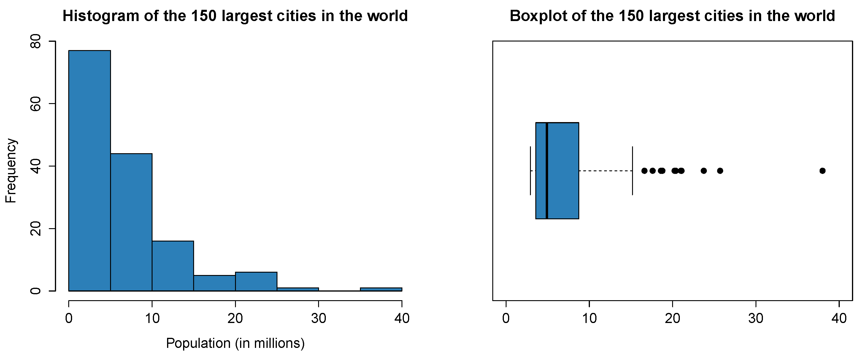
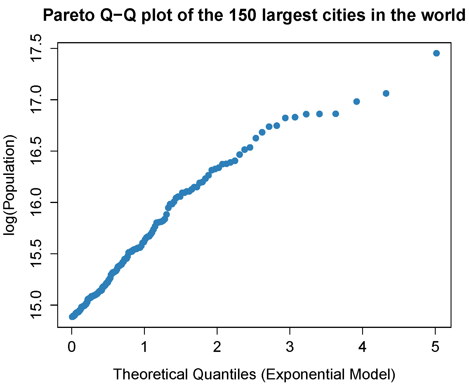
4.3.1. Population of the Largest Metropolitan Areas in the World
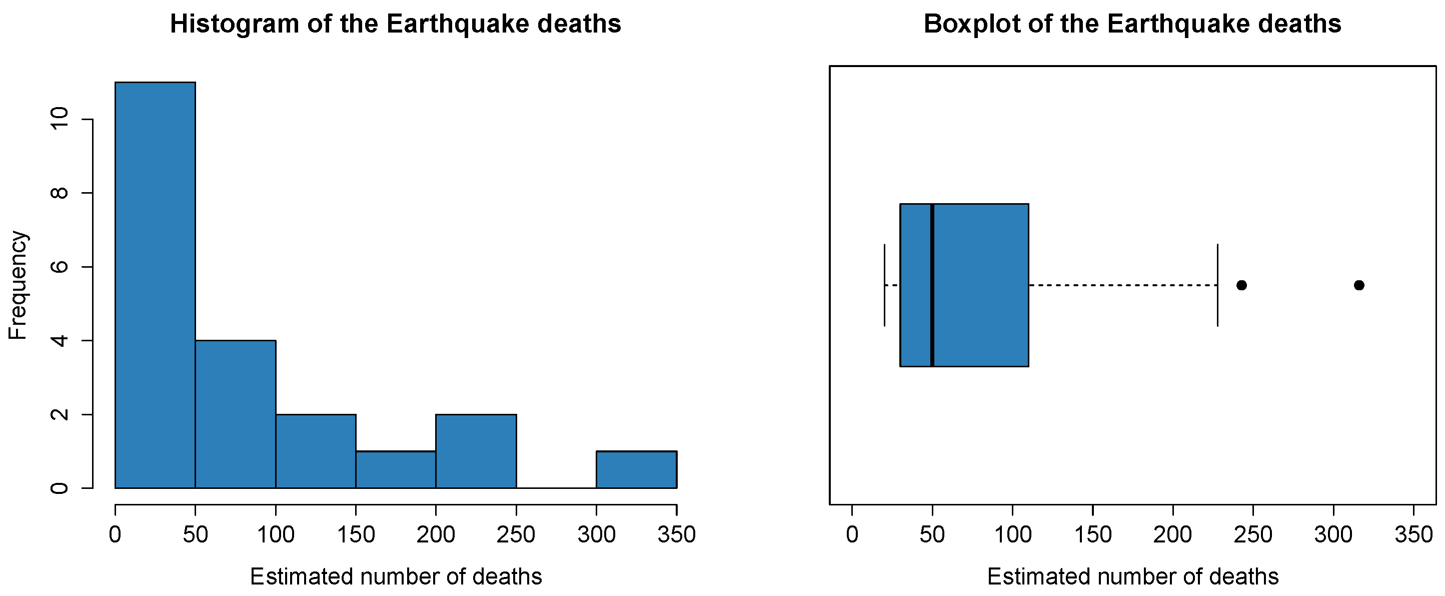
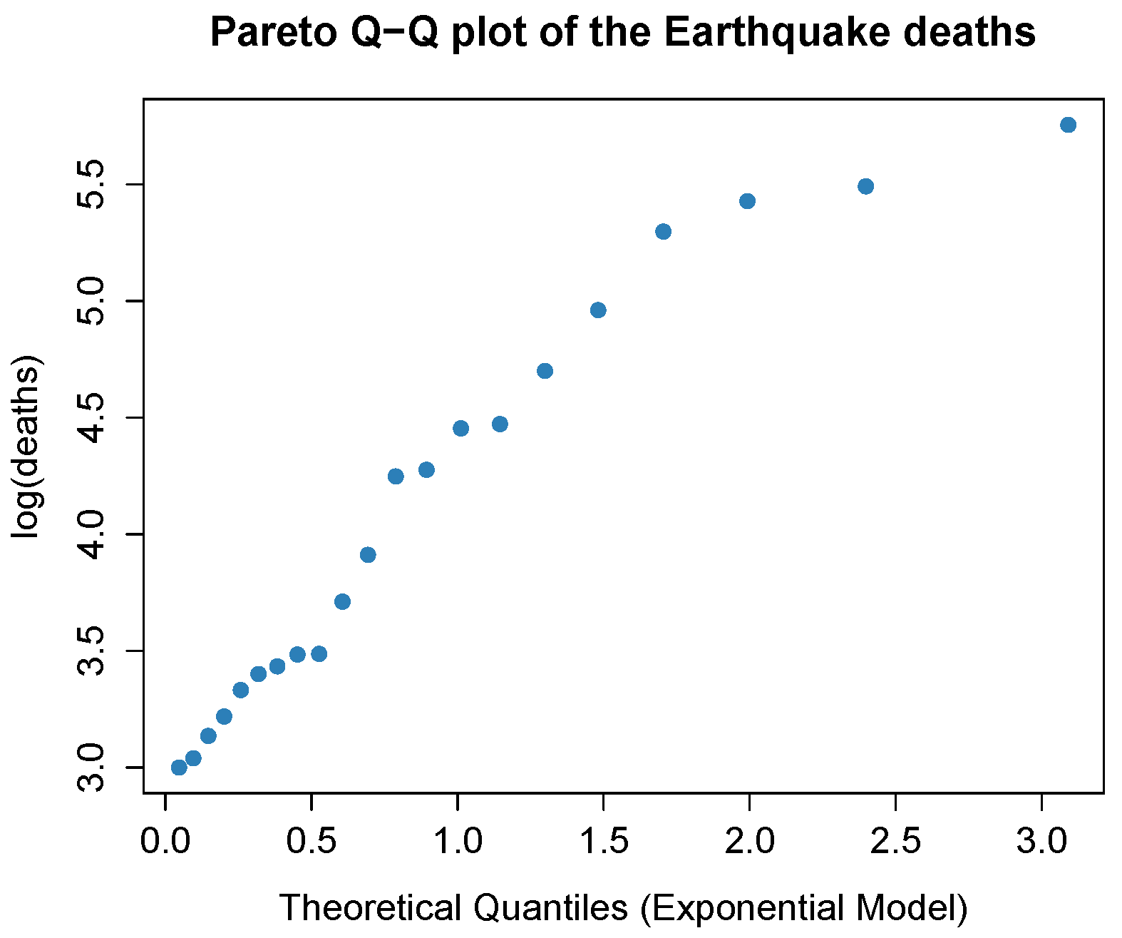
4.3.2. Estimated Number of Deaths in Major Earthquakes
5. Conclusions
Author Contributions
Funding
Data Availability Statement
Conflicts of Interest
Appendix A

| Rank | City | Country | Population | Rank | City | Country | Population |
|---|---|---|---|---|---|---|---|
| 1 | Tokyo | Japan | 38,001,000 | 76 | Abidjan | Cote d’Ivoire | 4,859,798 |
| 2 | Delhi | India | 25,703,168 | 77 | Guadalajara | Mexico | 4,843,241 |
| 3 | Shanghai | China | 23,740,778 | 78 | Yangon | Myanmar | 4,801,930 |
| 4 | São Paulo | Brazil | 21,066,245 | 79 | Alexandria | Egypt | 4,777,677 |
| 5 | Mumbai | India | 21,042,538 | 80 | Ankara | Turkey | 4,749,968 |
| 6 | Mexico City | Mexico | 20,998,543 | 81 | Kabul | Afghanistan | 4,634,875 |
| 7 | Beijing | China | 20,383,994 | 82 | Qingdao | China | 4,565,549 |
| 8 | Osaka | Japan | 20,237,645 | 83 | Chittagong | Bangladesh | 4,539,393 |
| 9 | Cairo | Egypt | 18,771,769 | 84 | Monterrey | Mexico | 4,512,572 |
| 10 | New York | United States | 18,593,220 | 85 | Sydney | Australia | 4,505,341 |
| 11 | Dhaka | Bangladesh | 17,598,228 | 86 | Dalian | China | 4,489,380 |
| 12 | Karachi | Pakistan | 16,617,644 | 87 | Xiamen | China | 4,430,081 |
| 13 | Buenos Aires | Argentina | 15,180,176 | 88 | Zhengzhou | China | 4,387,118 |
| 14 | Kolkata | India | 14,864,919 | 89 | Boston | United States | 4,249,036 |
| 15 | Istanbul | Turkey | 14,163,989 | 90 | Melbourne | Australia | 4,203,416 |
| 16 | Chongqing | China | 13,331,579 | 91 | Brasília | Brazil | 4,155,476 |
| 17 | Lagos | Nigeria | 13,122,829 | 92 | Jiddah | Saudi Arabia | 4,075,803 |
| 18 | Manila | Philippines | 12,946,263 | 93 | Phoenix | United States | 4,062,605 |
| 19 | Rio de Janeiro | Brazil | 12,902,306 | 94 | Ji’nan | China | 4,032,150 |
| 20 | Guangzhou | China | 12,458,130 | 95 | Montréal | Canada | 3,980,708 |
| 21 | Los Angeles | United States | 12,309,530 | 96 | Shantou | China | 3,948,813 |
| 22 | Moscow | Russia | 12,165,704 | 97 | Nairobi | Kenya | 3,914,791 |
| 23 | Kinshasa | D. Rep. Congo | 11,586,914 | 98 | Medellín | Colombia | 3,910,989 |
| 24 | Tianjin | China | 11,210,329 | 99 | Fortaleza | Brazil | 3,880,202 |
| 25 | Paris | France | 10,843,285 | 100 | Kunming | China | 3,779,558 |
| 26 | Shenzhen | China | 10,749,473 | 101 | Changchun | China | 3,762,390 |
| 27 | Jakarta | Indonesia | 10,323,142 | 102 | Changsha | China | 3,761,018 |
| 28 | London | United Kingdom | 10,313,307 | 103 | Recife | Brazil | 3,738,526 |
| 29 | Bangalore | India | 10,087,132 | 104 | Rome | Italy | 3,717,956 |
| 30 | Lima | Peru | 9,897,033 | 105 | Zhongshan | China | 3,691,360 |
| 31 | Chennai | India | 9,890,427 | 106 | Cape Town | South Africa | 3,660,447 |
| 32 | Seoul | South Korea | 9,773,746 | 107 | Detroit | United States | 3,639,050 |
| 33 | Bogotá | Colombia | 9,764,769 | 108 | Hanoi | Vietnam | 3,629,493 |
| 34 | Nagoya | Japan | 9,406,264 | 109 | Tel Aviv | Israel | 3,608,265 |
| 35 | Johannesburg | South Africa | 9,398,698 | 110 | Porto Alegre | Brazil | 3,602,526 |
| 36 | Bangkok | Thailand | 9,269,823 | 111 | Kano | Nigeria | 3,587,049 |
| 37 | Hyderabad | India | 8,943,523 | 112 | Salvador | Brazil | 3,582,967 |
| 38 | Chicago | United States | 8,744,835 | 113 | Faisalabad | Pakistan | 3,566,952 |
| 39 | Lahore | Pakistan | 8,741,365 | 114 | Berlin | Germany | 3,563,194 |
| 40 | Tehran | Iran | 8,432,196 | 115 | Aleppo | Syria | 3,561,796 |
| 41 | Wuhan | China | 7,905,572 | 116 | Dakar | Senegal | 3,520,215 |
| 42 | Chengdu | China | 7,555,705 | 117 | Casablanca | Morocco | 3,514,958 |
| 43 | Dongguan | China | 7,434,935 | 118 | Urumqi | China | 3,498,591 |
| 44 | Nanjing | China | 7,369,157 | 119 | Taiyuan | China | 3,481,810 |
| 45 | Ahmadabad | India | 7,342,850 | 120 | Curitiba | Brazil | 3,473,681 |
| 46 | Hong Kong | Hong Kong | 7,313,557 | 121 | Jaipur | India | 3,460,701 |
| 47 | Ho Chi Minh City | Vietnam | 7,297,780 | 122 | Shizuoka | Japan | 3,368,988 |
| 48 | Foshan | Foshan | 7,035,945 | 123 | Hefei | China | 3,347,591 |
| 49 | Kuala Lumpur | Malaysia | 6,836,911 | 124 | San Francisco | United States | 3,300,075 |
| 50 | Baghdad | Iraq | 6,642,848 | 125 | Fuzhou | China | 3,282,932 |
| 51 | Santiago | Chile | 6,507,400 | 126 | Shijiazhuang | China | 3,264,498 |
| 52 | Hangzhou | China | 6,390,637 | 127 | Seattle | United States | 3,248,724 |
| 53 | Riyadh | Saudi Arabia | 6,369,710 | 128 | Addis Ababa | Ethiopia | 3,237,525 |
| 54 | Shenyang | China | 6,315,470 | 129 | Nanning | China | 3,234,379 |
| 55 | Madrid | Spain | 6,199,254 | 130 | Lucknow | India | 3,221,817 |
| 56 | Xi’an | China | 6,043,700 | 131 | Busan | South Korea | 3,216,298 |
| 57 | Toronto | Canada | 5,992,739 | 132 | Wenzhou | China | 3,207,846 |
| 58 | Miami | United States | 5,817,221 | 133 | Ibadan | Nigeria | 3,160,190 |
| 59 | Pune | India | 5,727,530 | 134 | Ningbo | China | 3,131,921 |
| 60 | Belo Horizonte | Brazil | 5,716,422 | 135 | San Diego | United States | 3,107,034 |
| 61 | Dallas | United States | 5,702,641 | 136 | Milan | Italy | 3,098,974 |
| 62 | Surat | India | 5,650,011 | 137 | Yaounde | Cameroon | 3,065,692 |
| 63 | Houston | United States | 5,638,045 | 138 | Athens | Greece | 3,051,899 |
| 64 | Singapore | Singapore | 5,618,866 | 139 | Wuxi | China | 3,049,042 |
| 65 | Philadelphia | United States | 5,585,211 | 140 | Campinas | Brazil | 3,047,102 |
| 66 | Kitakyushu | Japan | 5,510,478 | 141 | Izmir | Turkey | 3,040,416 |
| 67 | Luanda | Angola | 5,506,000 | 142 | Kanpur | India | 3,020,795 |
| 68 | Suzhou | China | 5,472,033 | 143 | Mashhad | Iran | 3,014,424 |
| 69 | Haerbin | China | 5,457,414 | 144 | Puebla | Mexico | 2,984,048 |
| 70 | Barcelona | Spain | 5,258,319 | 145 | Sana’a | Yemen | 2,961,934 |
| 71 | Atlanta | United States | 5,142,140 | 146 | Santo Domingo | Domican Rep. | 2,945,353 |
| 72 | Khartoum | Sudan | 5,129,358 | 147 | Douala | Cameroon | 2,943,318 |
| 73 | Dar es Salaam | Tanzania | 5,115,670 | 148 | Kiev | Ukraine | 2,941,884 |
| 74 | Saint Petersburg | Russia | 4,992,991 | 149 | Guatemala City | Guatemala | 2,918,337 |
| 75 | Washington D.C. | United States | 4,955,139 | 150 | Caracas | Venezuela | 2,916,183 |
References
- Pareto, V. Cours d’Economie Politique; Librairie Droz: Lausanne, Switzerland, 1897; Volume 2. [Google Scholar]
- Kleiber, C.; Kotz, S. Statistical Size Distributions in Economics and Actuarial Sciences; John Wiley & Sons: Hoboken, NJ, USA, 2003; Volume 470. [Google Scholar] [CrossRef]
- Finkelstein, M.; Tucker, H.G.; Veeh, J.A. Pareto Tail Index Estimation Revisited. N. Am. Actuar. J. 2006, 10, 1–10. [Google Scholar] [CrossRef]
- Lomax, K.S. Business Failures: Another Example of the Analysis of Failure Data. J. Am. Stat. Assoc. 1954, 49, 847–852. [Google Scholar] [CrossRef]
- Bourguignon, M.; Gallardo, D.I.; Gómez, H.J. A Note on Pareto-Type Distributions Parameterized by Its Mean and Precision Parameters. Mathematics 2022, 10, 528. [Google Scholar] [CrossRef]
- Charpentier, A.; Flachaire, E. Pareto models for top incomes and wealth. J. Econ. Inequal. 2022, 20, 1–25. [Google Scholar] [CrossRef]
- Beirlant, J.; Goegebeur, Y.; Segers, J.; Teugels, J.L. Statistics of Extremes: Theory and Applications; John Wiley & Sons: Chichester, UK, 2004. [Google Scholar]
- Beirlant, J.; Caeiro, F.; Gomes, M.I. An overview and open research topics in statistics of univariate extremes. Revstat-Stat. J. 2012, 10, 1–31. [Google Scholar] [CrossRef]
- Albrecher, H.; Beirlant, J.; Teugels, J.L. Reinsurance: Actuarial and Statistical Aspects; John Wiley & Sons, Ltd.: Chichester, UK, 2017. [Google Scholar] [CrossRef]
- Gomes, M.I.; Guillou, A. Extreme value theory and statistics of univariate extremes: A review. Int. Stat. Rev. 2015, 83, 263–292. [Google Scholar] [CrossRef]
- Peng, L.; Qi, Y. Inference for Heavy-Tailed Data: Applications in Insurance and Finance; Academic Press: Cambridge, MA, USA, 2017. [Google Scholar] [CrossRef]
- Quandt, R.E. Old and new methods of estimation and the Pareto distribution. Metrika 1966, 10, 55–82. [Google Scholar] [CrossRef]
- Lu, H.L.; Tao, S.H. The Estimation of Pareto Distribution by a Weighted Least Square Method. Qual. Quant. 2007, 41, 913–926. [Google Scholar] [CrossRef]
- Caeiro, F.; Martins, A.P.; Sequeira, I.J. Finite sample behaviour of classical and quantile regression estimators for the Pareto distribution. AIP Conf. Proc. 2015, 1648, 540007. [Google Scholar] [CrossRef]
- Kantar, Y.M. Generalized least squares and weighted least squares estimation methods for distributional parameters. REVSTAT-Stat. J. 2015, 13, 263–282. [Google Scholar] [CrossRef]
- Kim, J.H.; Ahn, S.; Ahn, S. Parameter estimation of the Pareto distribution using a pivotal quantity. J. Korean Stat. Soc. 2017, 46, 438–450. [Google Scholar] [CrossRef]
- Brazauskas, V.; Serfling, R. Robust and Efficient Estimation of the Tail Index of a Single-Parameter Pareto Distribution. N. Am. Actuar. J. 2000, 4, 12–27. [Google Scholar] [CrossRef]
- Vandewalle, B.; Beirlant, J.; Christmann, A.; Hubert, M. A robust estimator for the tail index of Pareto-type distributions. Comput. Stat. Data Anal. 2007, 51, 6252–6268. [Google Scholar] [CrossRef]
- Arnold, B.C.; Press, S.J. Bayesian estimation and prediction for Pareto data. J. Am. Stat. Assoc. 1989, 84, 1079–1084. [Google Scholar] [CrossRef]
- Rasheed, H.A.; Al-Gazi, N.A.A. Bayes estimators for the shape parameter of Pareto type I distribution under generalized square error loss function. Math. Theory Model. 2014, 4, 20–32. [Google Scholar]
- Han, M. The E-Bayesian estimation and its E-MSE of Pareto distribution parameter under different loss functions. J. Stat. Comput. Simul. 2020, 90, 1834–1848. [Google Scholar] [CrossRef]
- Singh, V.P.; Guo, H. Parameter estimations for 2-parameter Pareto distribution by pome. Water Resour. Manag. 1995, 9, 81–93. [Google Scholar] [CrossRef]
- Caeiro, F.; Gomes, M.I. Semi-parametric tail inference through probability-weighted moments. J. Stat. Plan. Inference 2011, 141, 937–950. [Google Scholar] [CrossRef]
- Caeiro, F.; Gomes, M.I. A Class of Semi-parametric Probability Weighted Moment Estimators. In Recent Developments in Modeling and Applications in Statistics; Springer: Berlin/Heidelberg, Germany, 2013; pp. 139–147. [Google Scholar] [CrossRef]
- Munir, R.; Saleem, M.; Aslam, M.; Ali, S. Comparison of different methods of parameters estimation for Pareto Model. Casp. J. Appl. Sci. Res. 2013, 2, 45–56. [Google Scholar]
- Bhatti, S.H.; Hussain, S.; Ahmad, T.; Aslam, M.; Aftab, M.; Raza, M.A. Efficient estimation of Pareto model: Some modified percentile estimators. PLoS ONE 2018, 13, e0196456. [Google Scholar] [CrossRef] [PubMed]
- Bhatti, S.H.; Hussain, S.; Ahmad, T.; Aftab, M.; Ali Raza, M.; Tahir, M. Efficient estimation of Pareto model using modified maximum likelihood estimators. Sci. Iran. 2019, 26, 605–614. [Google Scholar] [CrossRef]
- Chen, W.; Yang, R.; Yao, D.; Long, C. Pareto parameters estimation using moving extremes ranked set sampling. Stat. Pap. 2019, 62, 1195–1211. [Google Scholar] [CrossRef]
- Greenwood, J.A.; Landwehr, J.M.; Matalas, N.C.; Wallis, J.R. Probability weighted moments: Definition and relation to parameters of several distributions expressable in inverse form. Water Resour. Res. 1979, 15, 1049–1054. [Google Scholar] [CrossRef]
- Hosking, J.R.M.; Wallis, J.R.; Wood, E.F. Estimation of the generalized extreme-value distribution by the method of probability-weighted moments. Technometrics 1985, 27, 251–261. [Google Scholar] [CrossRef]
- Jing, D.; Dedun, S.; Ronfu, Y.; Yu, H. Expressions relating probability weighted moments to parameters of several distributions inexpressible in inverse form. J. Hydrol. 1989, 110, 259–270. [Google Scholar] [CrossRef]
- Landwehr, J.M.; Matalas, N.; Wallis, J. Probability weighted moments compared with some traditional techniques in estimating Gumbel parameters and quantiles. Water Resour. Res. 1979, 15, 1055–1064. [Google Scholar] [CrossRef]
- Landwehr, J.M.; Matalas, N.; Wallis, J. Estimation of parameters and quantiles of Wakeby distributions: 1. Known lower bounds. Water Resour. Res. 1979, 15, 1361–1372. [Google Scholar] [CrossRef]
- Caeiro, F.; Gomes, M.I. Computational Study of the Adaptive Estimation of the Extreme Value Index with Probability Weighted Moments. In Proceedings of the Recent Developments in Statistics and Data Science: SPE2021, Évora, Portugal, 13–16 October 2021; Bispo, R., Henriques-Rodrigues, L., Alpizar-Jara, R., de Carvalho, M., Eds.; Springer International Publishing: Cham, Switzerland, 2022; pp. 29–39. [Google Scholar] [CrossRef]
- Caeiro, F.; Gomes, M.I.; Vandewalle, B. Semi-parametric probability-weighted moments estimation revisited. Methodol. Comput. Appl. Probab. 2014, 16, 1–29. [Google Scholar] [CrossRef]
- Rasmussen, P.F. Generalized probability weighted moments: Application to the generalized Pareto distribution. Water Resour. Res. 2001, 37, 1745–1751. [Google Scholar] [CrossRef]
- Caeiro, F.; Prata Gomes, D. A Log Probability Weighted Moment Estimator of Extreme Quantiles. In Theory and Practice of Risk Assessment; Springer Proceedings in Mathematics & Statistics; Kitsos, C., Oliveira, T., Rigas, A., Gulati, S., Eds.; Springer: Cham, Switzerland, 2015; Volume 136, pp. 293–303. [Google Scholar] [CrossRef]
- Caeiro, F.; Mateus, A. Log Probability Weighted Moments Method for Pareto distribution. In Proceedings of the 17th Applied Stochastic Models and Data Analysis International Conference with the 6th Demographics Workshop, London, UK, 6–9 June 2017; Skiadas, C.H., Ed.; 2017; pp. 211–218. [Google Scholar]
- Chen, H.; Cheng, W.; Zhao, J.; Zhao, X. Parameter estimation for generalized Pareto distribution by generalized probability weighted moment-equations. Commun. Stat.-Simul. Comput. 2017, 46, 7761–7776. [Google Scholar] [CrossRef]
- Mateus, A.; Caeiro, F. A new class of estimators for the shape parameter of a Pareto model. Comput. Math. Methods 2021, 3, e1133. [Google Scholar] [CrossRef]
- Mateus, A.; Caeiro, F. Confidence intervals for the shape parameter of a Pareto distribution. AIP Conf. Proc. 2022, 2425, 320003. [Google Scholar] [CrossRef]
- Arnold, B.C. Pareto and Generalized Pareto Distributions. In Modeling Income Distributions and Lorenz Curves; Chotikapanich, D., Ed.; Springer: New York, NY, USA, 2008; pp. 119–145. [Google Scholar] [CrossRef]
- Arnold, B.C.; Balakrishnan, N.; Nagaraja, H.N. A First Course in Order Statistics; Siam: Philadelphia, PA, USA, 1992; Volume 54. [Google Scholar] [CrossRef]
- Ahmad, M.I.; Sinclair, C.D.; Spurr, B.D. Assessment of flood frequency models using empirical distribution function statistics. Water Resour. Res. 1988, 24, 1323–1328. [Google Scholar] [CrossRef]
- Razali, N.M.; Wah, Y.B. Power Comparisons of Shapiro-Wilk, Kolmogorov-Smirnov, Lilliefors and Anderson-Darling Tests. J. Stat. Model. Anal. 2011, 2, 21–33. [Google Scholar]
- Singla, N.; Jain, K.; Kumar Sharma, S. Goodness of Fit Tests and Power Comparisons for Weighted Gamma Distribution. REVSTAT-Stat. J. 2016, 14, 29–48. [Google Scholar] [CrossRef]
- The 150 Largest Cities in the World. Available online: https://www.worldatlas.com/citypops.htm (accessed on 15 May 2021).
- Bowley, A.L. Elements of Statistics; PS King & Son: London, UK, 1901. [Google Scholar]
- Horn, P.S. Robust quantile estimators for skewed populations. Biometrika 1990, 77, 631–636. [Google Scholar] [CrossRef]
- Kim, T.H.; White, H. On more robust estimation of skewness and kurtosis. Financ. Res. Lett. 2004, 1, 56–73. [Google Scholar] [CrossRef]
- Brys, G.; Hubert, M.; Struyf, A. A Robust Measure of Skewness. J. Comput. Graph. Stat. 2004, 13, 996–1017. [Google Scholar] [CrossRef]
- Cirillo, P. Are your data really Pareto distributed? Phys. A Stat. Mech. Its Appl. 2013, 392, 5947–5962. [Google Scholar] [CrossRef]
- Clark, D. A Note on the Upper-truncated Pareto distribution. Casualty Actuar. Soc. E-Forum 2013, Winter 1, 1–22. [Google Scholar]


| ML | M | PWM | LGPWM-KS | LGPWM-CvM | LGPWM-MAD | |
|---|---|---|---|---|---|---|
| Bias/RMSE | Bias/RMSE | Bias/RMSE | Bias/RMSE | Bias/RMSE | Bias/RMSE | |
| Pareto model with and | ||||||
| 15 | 0.016/0.037 | 0.900/0.900 | 0.906/0.906 | 0.014/0.042 | 0.015/0.041 | 0.008/0.036 |
| 20 | 0.012/0.030 | 0.900/0.900 | 0.904/0.904 | 0.010/0.030 | 0.010/0.032 | 0.006/0.029 |
| 30 | 0.007/0.020 | 0.900/0.900 | 0.903/0.903 | 0.006/0.023 | 0.005/0.022 | 0.003/0.021 |
| 40 | 0.006/0.019 | 0.900/0.900 | 0.902/0.902 | 0.006/0.022 | 0.005/0.022 | 0.003/0.020 |
| 50 | 0.004/0.014 | 0.900/0.900 | 0.902/0.902 | 0.004/0.016 | 0.004/0.016 | 0.002/0.015 |
| 75 | 0.003/0.011 | 0.900/0.900 | 0.901/0.901 | 0.003/0.013 | 0.002/0.013 | 0.001/0.012 |
| 100 | 0.002/0.010 | 0.900/0.900 | 0.901/0.901 | 0.003/0.011 | 0.002/0.012 | 0.001/0.011 |
| 150 | 0.001/0.008 | 0.900/0.900 | 0.901/0.901 | 0.002/0.009 | 0.001/0.009 | 0.000/0.009 |
| 200 | 0.001/0.007 | 0.900/0.900 | 0.900/0.900 | 0.001/0.008 | 0.001/0.008 | 0.000/0.008 |
| Pareto model with and | ||||||
| 15 | 0.040/0.093 | 0.753/0.753 | 0.776/0.778 | 0.036/0.106 | 0.037/0.103 | 0.020/0.089 |
| 20 | 0.029/0.074 | 0.751/0.751 | 0.770/0.770 | 0.025/0.076 | 0.026/0.081 | 0.016/0.072 |
| 30 | 0.017/0.050 | 0.750/0.750 | 0.763/0.764 | 0.015/0.058 | 0.012/0.055 | 0.008/0.051 |
| 40 | 0.015/0.047 | 0.750/0.750 | 0.759/0.759 | 0.014/0.054 | 0.013/0.054 | 0.009/0.049 |
| 50 | 0.011/0.036 | 0.750/0.750 | 0.757/0.757 | 0.011/0.041 | 0.010/0.041 | 0.006/0.038 |
| 75 | 0.007/0.027 | 0.750/0.750 | 0.754/0.754 | 0.008/0.032 | 0.006/0.033 | 0.003/0.030 |
| 100 | 0.006/0.025 | 0.750/0.750 | 0.753/0.753 | 0.006/0.029 | 0.005/0.029 | 0.002/0.027 |
| 150 | 0.003/0.020 | 0.750/0.750 | 0.752/0.752 | 0.004/0.023 | 0.003/0.023 | 0.001/0.022 |
| 200 | 0.002/0.017 | 0.750/0.750 | 0.752/0.752 | 0.003/0.020 | 0.002/0.020 | 0.000/0.020 |
| Pareto model with and | ||||||
| 15 | 0.120/0.280 | 0.429/0.467 | 0.524/0.577 | 0.118/0.318 | 0.115/0.309 | 0.069/0.277 |
| 20 | 0.088/0.223 | 0.397/0.422 | 0.479/0.524 | 0.089/0.238 | 0.086/0.252 | 0.052/0.219 |
| 30 | 0.052/0.151 | 0.363/0.375 | 0.435/0.463 | 0.051/0.180 | 0.040/0.166 | 0.025/0.155 |
| 40 | 0.046/0.141 | 0.346/0.357 | 0.401/0.421 | 0.048/0.167 | 0.042/0.163 | 0.027/0.146 |
| 50 | 0.033/0.107 | 0.330/0.338 | 0.379/0.398 | 0.036/0.122 | 0.033/0.124 | 0.019/0.114 |
| 75 | 0.021/0.080 | 0.315/0.319 | 0.354/0.364 | 0.026/0.099 | 0.020/0.098 | 0.009/0.090 |
| 100 | 0.018/0.075 | 0.310/0.314 | 0.347/0.355 | 0.021/0.087 | 0.015/0.087 | 0.008/0.081 |
| 150 | 0.010/0.059 | 0.301/0.304 | 0.333/0.340 | 0.014/0.071 | 0.008/0.069 | 0.003/0.067 |
| 200 | 0.007/0.052 | 0.297/0.300 | 0.327/0.332 | 0.010/0.060 | 0.006/0.060 | 0.001/0.059 |
| Pareto model with and | ||||||
| 15 | 0.160/0.373 | 0.363/0.462 | 0.475/0.593 | 0.138/0.410 | 0.143/0.410 | 0.077/0.354 |
| 20 | 0.118/0.298 | 0.318/0.393 | 0.416/0.519 | 0.097/0.299 | 0.098/0.318 | 0.063/0.289 |
| 30 | 0.069/0.202 | 0.269/0.316 | 0.356/0.429 | 0.054/0.227 | 0.047/0.218 | 0.029/0.206 |
| 40 | 0.061/0.188 | 0.244/0.291 | 0.309/0.370 | 0.054/0.216 | 0.052/0.216 | 0.034/0.195 |
| 50 | 0.044/0.143 | 0.217/0.256 | 0.276/0.335 | 0.041/0.160 | 0.041/0.164 | 0.024/0.152 |
| 75 | 0.028/0.107 | 0.195/0.221 | 0.244/0.282 | 0.029/0.129 | 0.025/0.130 | 0.011/0.119 |
| 100 | 0.024/0.100 | 0.190/0.213 | 0.236/0.270 | 0.024/0.115 | 0.019/0.116 | 0.010/0.108 |
| 150 | 0.013/0.078 | 0.173/0.193 | 0.214/0.245 | 0.016/0.092 | 0.011/0.094 | 0.004/0.090 |
| 200 | 0.009/0.069 | 0.167/0.186 | 0.205/0.232 | 0.011/0.079 | 0.008/0.080 | 0.001/0.080 |
| ML | M | PWM | LGPWM-KS | LGPWM-CvM | LGPWM-MAD | |
|---|---|---|---|---|---|---|
| Bias/RMSE | Bias/RMSE | Bias/RMSE | Bias/RMSE | Bias/RMSE | Bias/RMSE | |
| Pareto model with and | ||||||
| 15 | 0.517/2.489 | 0.466/2.319 | */* | 0.428/1.439 | 0.525/1.852 | 0.366/1.248 |
| 20 | 0.199/0.350 | 0.176/0.326 | */* | 0.345/1.376 | 0.328/1.362 | 0.294/1.193 |
| 30 | 0.111/0.200 | 0.099/0.189 | */* | 0.097/0.302 | 0.112/0.470 | 0.100/0.384 |
| 40 | 0.077/0.131 | 0.069/0.124 | */* | 0.064/0.221 | 0.066/0.262 | 0.066/0.279 |
| 50 | 0.059/0.087 | 0.053/0.082 | */* | 0.058/0.204 | 0.060/0.219 | 0.051/0.216 |
| 75 | 0.036/0.052 | 0.032/0.050 | */* | 0.025/0.113 | 0.022/0.127 | 0.025/0.217 |
| 100 | 0.025/0.035 | 0.022/0.033 | */* | 0.018/0.088 | 0.013/0.089 | 0.011/0.117 |
| 150 | 0.016/0.021 | 0.014/0.020 | */* | 0.012/0.069 | 0.009/0.084 | 0.008/0.103 |
| 200 | 0.012/0.016 | 0.010/0.015 | */* | 0.009/0.062 | 0.004/0.061 | 0.001/0.079 |
| Pareto model with and | ||||||
| 15 | 0.179/0.335 | 0.134/0.296 | */* | 0.122/0.345 | 0.133/0.381 | 0.086/0.332 |
| 20 | 0.112/0.168 | 0.081/0.144 | */* | 0.095/0.303 | 0.093/0.299 | 0.071/0.301 |
| 30 | 0.070/0.108 | 0.051/0.094 | */* | 0.043/0.149 | 0.039/0.173 | 0.028/0.180 |
| 40 | 0.052/0.078 | 0.039/0.068 | */* | 0.029/0.119 | 0.026/0.128 | 0.019/0.147 |
| 50 | 0.042/0.059 | 0.031/0.051 | */* | 0.025/0.114 | 0.025/0.121 | 0.013/0.133 |
| 75 | 0.026/0.037 | 0.019/0.032 | */* | 0.011/0.078 | 0.007/0.083 | 0.001/0.111 |
| 100 | 0.019/0.026 | 0.014/0.022 | */* | 0.009/0.063 | 0.004/0.065 | −0.001/0.081 |
| 150 | 0.012/0.016 | 0.009/0.014 | */* | 0.007/0.052 | 0.003/0.057 | −0.001/0.071 |
| 200 | 0.009/0.013 | 0.007/0.011 | */* | 0.004/0.046 | 0.000/0.047 | −0.005/0.060 |
| Pareto model with and | ||||||
| 15 | 0.048/0.073 | 0.016/0.054 | 0.514/2.059 | 0.034/0.084 | 0.034/0.084 | 0.018/0.090 |
| 20 | 0.033/0.046 | 0.009/0.033 | 0.356/0.720 | 0.028/0.072 | 0.026/0.074 | 0.014/0.078 |
| 30 | 0.021/0.031 | 0.006/0.023 | 0.370/0.682 | 0.015/0.045 | 0.012/0.046 | 0.006/0.054 |
| 40 | 0.016/0.023 | 0.004/0.017 | 0.321/0.456 | 0.011/0.037 | 0.008/0.038 | 0.003/0.045 |
| 50 | 0.013/0.018 | 0.004/0.013 | 0.316/0.409 | 0.009/0.036 | 0.007/0.036 | 0.002/0.043 |
| 75 | 0.009/0.012 | 0.002/0.008 | 0.302/0.346 | 0.004/0.026 | 0.002/0.027 | −0.001/0.034 |
| 100 | 0.006/0.008 | 0.001/0.006 | 0.306/0.349 | 0.004/0.021 | 0.002/0.021 | −0.001/0.026 |
| 150 | 0.004/0.005 | 0.001/0.004 | 0.299/0.321 | 0.002/0.017 | 0.001/0.017 | −0.001/0.023 |
| 200 | 0.003/0.004 | 0.001/0.003 | 0.308/0.329 | 0.002/0.015 | −0.000/0.016 | −0.002/0.020 |
| Pareto model with and | ||||||
| 15 | 0.070/0.105 | 0.015/0.075 | 0.293/0.625 | 0.033/0.120 | 0.035/0.122 | 0.011/0.131 |
| 20 | 0.048/0.068 | 0.010/0.047 | 0.238/0.343 | 0.026/0.102 | 0.024/0.103 | 0.009/0.114 |
| 30 | 0.032/0.046 | 0.004/0.032 | 0.233/0.328 | 0.012/0.063 | 0.009/0.068 | 0.002/0.080 |
| 40 | 0.024/0.034 | 0.003/0.024 | 0.198/0.262 | 0.008/0.053 | 0.007/0.056 | 0.001/0.067 |
| 50 | 0.020/0.027 | 0.003/0.018 | 0.183/0.239 | 0.007/0.052 | 0.007/0.054 | −0.000/0.064 |
| 75 | 0.013/0.018 | 0.001/0.012 | 0.173/0.215 | 0.002/0.037 | 0.000/0.040 | −0.004/0.052 |
| 100 | 0.009/0.012 | 0.001/0.008 | 0.173/0.209 | 0.002/0.030 | 0.000/0.031 | −0.003/0.040 |
| 150 | 0.006/0.008 | 0.000/0.005 | 0.165/0.193 | 0.001/0.025 | −0.000/0.027 | −0.003/0.034 |
| 200 | 0.005/0.006 | 0.000/0.004 | 0.163/0.184 | 0.001/0.023 | −0.001/0.024 | −0.004/0.030 |
| Min. | 1st Quart. | Median | Mean | 3rd Quart. | Max. |
|---|---|---|---|---|---|
| 2.916 | 3.571 | 4.907 | 7.082 | 8.744 | 38.001 |
| ML | 1.4599 | 2.9162 | 0.0595 | 0.0979 | 0.4462 |
| M | 1.6953 | 2.9047 | 0.1167 | 0.5929 | 2.1937 |
| PWM | 1.8835 | 3.3222 | 0.1800 | 0.9749 | 2.1406 |
| LGPWM () | 1.3933 | 2.9129 | 0.0437 | 0.0529 | 0.3408 |
| LGPWM () | 1.3325 | 2.8694 | 0.0502 | 0.0408 | 0.3686 |
| LGPWM () | 1.3824 | 2.9056 | 0.0447 | 0.0488 | 0.3398 |
| Min. | 1st Quart. | Median | Mean | 3rd Quart. | Max. |
|---|---|---|---|---|---|
| 20.09 | 30.00 | 50.00 | 89.96 | 110.00 | 316.00 |
| ML | 0.9034 | 20.0850 | 0.1525 | 0.0615 | 0.2479 |
| M | 1.2737 | 19.3341 | 0.2820 | 0.4347 | 1.7498 |
| PWM | 1.5046 | 30.1704 | 0.3145 | 0.5197 | 1.1743 |
| LGPWM () | 0.7536 | 18.0595 | 0.1159 | 0.0520 | 0.2421 |
| LGPWM () | 0.8149 | 19.0483 | 0.1300 | 0.0467 | 0.2179 |
| LGPWM () | 0.8323 | 19.3380 | 0.1334 | 0.0468 | 0.2161 |
Disclaimer/Publisher’s Note: The statements, opinions and data contained in all publications are solely those of the individual author(s) and contributor(s) and not of MDPI and/or the editor(s). MDPI and/or the editor(s) disclaim responsibility for any injury to people or property resulting from any ideas, methods, instructions or products referred to in the content. |
© 2023 by the authors. Licensee MDPI, Basel, Switzerland. This article is an open access article distributed under the terms and conditions of the Creative Commons Attribution (CC BY) license (https://creativecommons.org/licenses/by/4.0/).
Share and Cite
Caeiro, F.; Mateus, A. A New Class of Generalized Probability-Weighted Moment Estimators for the Pareto Distribution. Mathematics 2023, 11, 1076. https://doi.org/10.3390/math11051076
Caeiro F, Mateus A. A New Class of Generalized Probability-Weighted Moment Estimators for the Pareto Distribution. Mathematics. 2023; 11(5):1076. https://doi.org/10.3390/math11051076
Chicago/Turabian StyleCaeiro, Frederico, and Ayana Mateus. 2023. "A New Class of Generalized Probability-Weighted Moment Estimators for the Pareto Distribution" Mathematics 11, no. 5: 1076. https://doi.org/10.3390/math11051076
APA StyleCaeiro, F., & Mateus, A. (2023). A New Class of Generalized Probability-Weighted Moment Estimators for the Pareto Distribution. Mathematics, 11(5), 1076. https://doi.org/10.3390/math11051076