Periodic Behavioral Routine Discovery Based on Implicit Spatial Correlations for Smart Home

Abstract

As the degree of elders’ social activity and self-care ability depreciates, the potential risk for elderly people who live independently increases. The development of assistive services such as smart homes could likely provide them with a safer living environment. These systems collect sensor data to monitor residents’ daily activities and provide assistance services accordingly. In order to do so, a smart home must understand its residents’ daily activities and identify their periodic behavioral daily routine accordingly. However, existing solutions mainly focus on the temporal feature of daily activities and require prior labeling of where sensors are geographically deployed. In this study, we extract implicit spatial information from hidden correlations between sensors deployed in the environment and present a concept of virtual locations that establishes an abstract spatial representation of the physical living space so that prior labeling of the actual location of the sensors is not required. To demonstrate the viability of this concept, an unsupervised periodic behavioral routine discovery method that does not require any predefined location-specific sensor data for a smart home environment is proposed. The experimental results show that with the help of virtual location, the proposed method achieves high accuracy in activity discovery and significantly reduces the computation time required to complete the task relative to a system without virtual location. Furthermore, the result of simulated anomaly detection also shows that the periodic behavioral routine discovery system is more tolerant to differences in the way routines are performed.

1. Introduction

Internet of Things (IoT) technologies offer a variety of applications [1] that may be beneficial to everyone due to their ability to allows connected devices to interact with other devices or sensors to collect and exchange data in real time. This creates a new context of data that may contain important information that can be used in many ways to improve the quality of life of the general population, for instance, monitoring the daily activities of the elderly using wearable and ambient sensors, tracking drugs through the supply chain by attaching smart labels to them [1], and controlling a robotic wheelchair using a joystick and flex sensor for disabled people [2]. Furthermore, there is an upward trend in the number of elderly people living independently at home [3,4]. A similar trend has also been reported, i.e., that elders prefer to stay at home alone due to the need for privacy, the high cost of hiring nurses, or inadequate medical resources [5]. Thus, the need for independent living has motivated many researchers to accelerate the development of smart home monitoring and automation techniques. For example, smart homes provide residents comfort, convenience, and energy efficiency via remote control and automation features. This technology can also be used to enhance the safety of residents and assist with independent living or elder care by tracking the daily activities of elders in the environment [6,7] or customizing load-shifting and energy-saving suggestions according to residents’ daily occupancy patterns [8]. The authors of [9] present a use case for a smartphone-based augmented reality application that allows the resident to control their smart devices via home automation. More importantly, health-assistive smart homes provide assistance to the elderly to track their physical and mental health status, which may extend their time to live independently in their preferred environment [10]. Considering the contextual information collected from different sensing sources, spatial information, e.g., the resident’s location, is very important to ensure the quality of service provided to residents [11] The resident’s current location in the environment is very useful when investigating their behavior patterns, and it is strongly related to activities performed in their daily life. For instance, activity recognition in a smart home learns residents’ movement patterns based on spatial reasoning. Smart home systems can then provide automated control of different aspects in relevant areas according to residents’ whereabouts that satisfy their daily routine needs. Furthermore, by inferring activities that deviate from daily routine, residents’ behavioral anomalies can be identified to notify and alert residents. To do so, residents’ activities must first be recognized to provide these services. Thus, finding suitable solutions that are viable for recognizing spatial information in a smart home is becoming increasingly important to support the growing aging population [12].

In [13], various sensors such as electromagnetic door contacts and infrared motion sensors were deployed around the environment to capture and collect data in a non-invasive manner when changes were detected. Sensors are usually strategically deployed in a particular location to carry out their tasks, and it is often necessary to know where sensors are deployed in order to track the whereabouts of residents. This requires labeling the deployment location of the sensors in advance (e.g., “motion sensor in the living room”, “door sensor at main entrance”) or assuming that predefined location-specific sensor data are applied [14]. This is either done by a professional installer or manually defined by users [15], which can result in errors in cases of users with no experience. Moreover, data labeling is time-consuming and annoying, and these labels can be unreliable [16]. The authors of [17] discovered that some data in a specific dataset were either unlabeled or contain spurious activities because the data were manually labeled by the resident, and imprecision and labeling noise may occur, increasing the difficulties of applying smart home monitoring techniques to realistic environments. To alleviate this problem, in this study, we propose an approach for periodic behavioral routine discovery that utilizes the virtual location concept to fill the gap in the works of the related literature. The idea is to extract implicit spatial information using hidden correlations between sensors deployed in the smart home environment and divide sensors into clusters called virtual locations based on the correlations among sensors and sensor types. This provides an abstract spatial representation of where sensors are deployed in the smart home environment and assigns a conceptual location to each sensor. For instance, a resident in a smart home environment may trigger a number of sensors while performing their daily activities. As the resident triggers a sensor, a nearby sensor may also be triggered soon after. This indicates a strong correlation between these sensors, which implies that they are likely to be physically close to each other.

The characteristics of different sensors may provide different types of knowledge about the environment. For example, the division of spaces can be inferred by a door contact sensor, and the occurrence of an activity or movement between different spaces in a specific region can be acquired by motion detectors. Thus, utilizing different types of sensors and knowledge of sensor correlations, it is possible to estimate the resident’s location as sensors are being triggered and compose their movement patterns. To validate the viability of this concept, in this study, we propose an unsupervised approach to discover periodic behavioral routines in a smart home where predefined location-specific sensor data are unavailable. The result of this approach can be further utilized to provide automation rules to assist with controlling different aspects of the smart home environment or to identify behavioral anomalies that deviate from periodic behavioral routines.

The main contributions of this study are summarized as follows.

• Abstract spatial representations of the physical living space are established, i.e., virtual location, which utilize the sensor correlations created by the occurrence and sequence of events. Virtual location does not need predefined or prior labeling of sensor locations in the environment. Our method provides an alternative solution for situations in which sensor locations are not available.
• A weighted graph is constructed to model the temporal correlations between sensors. Time differences between events can be calculated used to analyze the time correlation between any two sensors. A weight function is adopted to adjust the weight of correlations according to the sensor type.
• A method to determine transitional probability is developed to determine the probable transitions between activities. A strict sequence of periodic behavioral routines may be challenging, as the formation of the same routine may be irregular or inconsistent. Thus, transitional probability allows for limited deviations from periodic behavioral routines, which may facilitate the identification of daily activities and routine formation.
• We experimentally explore the validity of the concept of virtual location and demonstrate that this concept works well in a smart home environment without prior knowledge of where sensors are deployed. Hence, the proposed method offers great flexibility in the deployment of sensors in smart homes and can be suitably applied in real situations in which sensor deployment and space division differ.

The remainder of this study is organized as follows. In Section 2, we present the concepts and technologies used in the proposed method. In Section 3, we describe the proposed method and system architecture and provide details about each component when utilized in a smart home application. In Section 4, we present the evaluation methods, the experimental setup, and the experimental results of the proposed method. Finally, in Section 5, we draw conclusions.

2. Related Work

This study explores the value of the virtual location concept to smart home applications and practical deployments. There are various methods and techniques for detecting and monitoring people in an indoor environment, each of which has pros and cons. This study summarizes existing work related to three primary research directions: (1) location tracking, (2) activity recognition, and (3) graph clustering. In this study, we draw upon ideas and methods from these categories.

2.1. Location Tracking

Unique context information called user location [18] has gained recognition for its essential role in the smart home environment [19]. Activity recognition is commonly employed using sensors deployed in a smart home environment or as wearable sensors worn by the resident [20]. These sensors provide location information regarding where the resident triggers sensors. However, most existing solutions do not take spatial aspects into account or incorporate them in a minimal way [21,22]. For example, a smartphone-based localization method was proposed in [23] to explore the logical location of users. This includes using smartphone features such as accelerometers, microphones, cameras, and Wi-Fi to extract information about the sound, color, and lighting of the environment, as well as the user’s motion. The authors of [24] conducted a study to estimate the user’s location using an active sound-probing technique with a built-in speaker and microphone on a smartphone to adaptively disable image capture devices to protect privacy in a public restroom. The authors of [25] designed an active sensing system that utilizes acoustic signatures based on predesigned beep signals emitted by a smartphone to identify location semantics via echoes reflected from different static reflectors. The authors of [26] used stationary objects inside a building, such as pillars, railings, walls, doorways, and electrical equipment, to detect magnetic fingerprints using a magnetometer in a smartphone to perform indoor localization. The authors of [27] developed a system to monitor and assist the elderly in their daily activities using an RFID system for indoor localization. The patient wore multiple active tags, and RFID readers were placed on the walls to detect the patient’s whereabouts. The authors of [28] proposed a crowdsourcing approach to build an indoor positioning and navigation map utilizing Wi-Fi received signal strength (RSS) samples collected by the user’s mobile devices in combination with landmarks to detect and calibrate user location. Some studies require predefined location of sensors to provide location-specific sensor data and enable location prediction [14]. On the other hand, sensors that monitor and track users’ whereabouts using imagery and acoustics are usually perceived as intrusive [29]. Furthermore, providing predefined location-specific sensor data or labeling the location of sensors manually may be very time-consuming because labeling data for training is often an expensive process [16].

2.2. Activity Discovery

Activity discovery (AD) [30] is a data mining process for the discovery of interesting patterns by finding sets of events that frequently occur in sensor data. An example of AD is the episode discovery (ED) Algorithm [31]. An episode is a set of events, and the goal of ED is to identify episodes with a number of occurrences greater than a predefined threshold in an event sequence. An approach based on the minimum description length principle [32] is one example of an ED algorithm. The concept of this approach is that the model with the shortest description is the best model describing the data. ED replaces the occurrences of the episodes with pointers to obtain a more compact representation. ED runs the following steps iteratively: (1) generate a list of candidate episodes; (2) discover the periodicity of each candidate episode; (3) the episode that allows the shortest representation is identified as the pattern of interest. Details of ED are as follows.

First, ED processes the event sequence ($D=\left\{d_1,d_2,\dots ,d_n\right\}$) generated by sensors using a sliding window with a predefined length to collect candidate episodes. An episode ($E=\left\{e_1,e_2,\dots ,e_m\right\}$) occurs if there are $m$ events that match the $m$ events in $d_k\in D$. Formally, there is an occurrence of ($o$) of episode $E=\left\{e_1,e_2,\dots ,e_a\right\}$ at time $t_1$ if permutation $\sigma$ exists in $\left(1,\dots ,a\right)$, and timestamp $a$ is $t_1\le t_2\le \dots \le t_a$, such that $\left\{\left(e_{\sigma \left(1\right)},t_1\right),\dots , \left(e_{\sigma \left(a\right)},t_a\right)\right\}$ is a subsequence of $d_k=\left\{\left(e_1,t_1\right),\dots ,\left(e_b,t_b\right)\right\}$, where $a\le b$ and $d_k\in D$.

After obtaining occurrences of each episode, two periodicities are estimated with different time granularities: fine-grained and coarse-grained, indicating that the number of occurrences is truncated to an hour and a day, respectively. The periodicity of an episode is calculated based on repeating cycles of time differences between episodes. In ED, the periodicities of episode $E$ are estimated as follows.

• Obtain timestamps of occurrences of $E$: $t_1,t_2,\dots ,t_n$;
• Truncate the timestamps to an hour or a day according to the time granularity: $t_1^{\prime },t_2^{\prime },\dots ,t_n^{\prime }$;
• Calculate the time difference between timestamps: $\delta t_1,\delta t_2,\dots ,\delta t_{n-1}$;
• Estimate the length ($l$) of the repeating cycle of time differences between episodes using an autocorrelation measure.

The timestamps of occurrences of $E$ are processed according to the length ($l$) of the repeating cycle. For each sequence of $l$ time differences ($\delta t_k,\delta t_{k+1},\dots ,\delta t_{k+l-1}$), check whether $\delta t_k$ is matched against $\delta t_{k+l}$, $\delta t_{k+1}$ is matched against $\delta t_{k+l+1}$, etc. The occurrence is marked as a mistake when the time difference does not match the expected occurrence, and the periodicity is recalculates the time differences for the next sequence of $l$. Finally, rewrite the data using the periodicity information and select the episode with the shortest data length as the desired pattern. ED was proven effective in the MavHome project [33]. However, it lacks flexibility with respect to the time occurrence of episodes. Furthermore, when unexpected events are marked as mistakes, some important episodes of interest are not considered. Moreover, several articles have introduced probability and machine learning techniques to perform the AD process in a smart home environment. For instance, the authors of [34] proposed a global method based on probabilistic finite-state automata based on the knowledge of the training event logs database and a hierarchical decomposition of activities to monitor actions and moves to conduct AD automatically. A perplexity evaluation utilizing the normalized likelihood is adopted to select the most probable activities of daily living in activity recognition. The authors of [35] introduced a smart home control platform that analyzes the historical usage records of home automation devices to detect residents’ behavior patterns through sensors and IoT devices. The machine learning C4.5 algorithm was applied to generate a decision tree for automatic configuration of devices adjusted according to the user’s preferences.

2.3. Graph Clustering

Graph clustering (GC) is a process that discovers sets of related vertices with specific properties in a graph ($G=\left(V, W\right)$) with vertices ($V$) and edges ($W$). GC has been proven effective in various domains, e.g., computer vision, biology, and social sciences. The authors of [36] divided GC methods into five main types:

• Cohesive subgraph discovery: Search the desired partition with specific structural properties that subgraphs should satisfy under a certain condition, e.g., n-cliques and k-cores;
• Vertex clustering: Place vertices in a vector space where the pairwise distance between every two vertices can be computed or map the vertices to points in a low-dimensional space using the spectrum of the graph. Then, the graph clustering problem can be solved by traditional clustering methods, e.g., k-means and agglomerative hierarchical clustering;
• Quality optimization: This method optimizes some graph-based measures of partition quality, such as normalized cut, modularity optimization, and spectral optimization;
• Divisive: Iteratively identify the edges or vertices positioned between clusters, e.g., min-cut and max-flow;
• Model-based: Consider an underlying statistical model that can generate partitions of the graph, e.g., the Markov cluster algorithm.

The authors of [37] introduced a community detection method that employs local similarity to form communities by performing similarity measurements between nodes and their neighbors. Then, it utilizes degree clustering information that combines the local neighborhood ratio with the degree ratio. A large number of nodes with a low degree must adopt fewer nodes with a high degree, and each node in small-scale communities must attempt to connect the nodes with a high degree to expand communities. The authors of [38] proposed a community detection algorithm that utilizes the idea of graph clustering and iteratively applies min-cut to divide a community into two smaller communities. Modularity is used after each division as a stopping criterion to stop iterations of community division. In this study, we aim to identify sets of vertices with a high correlation when the number of clusters is not provided in advance. Thus, this study extends the Louvain method for graph clustering. The Louvain method is one of the modularity optimization methods proposed in [39]. It has been proven to outperform many similar optimization methods in terms of both modularity and the cost of time [40].

3. Virtual Location-Based Periodic Behavioral Routine Discovery

In this study, a novel concept called virtual location is introduced and was utilized to discover behavioral routines performed by a resident without prior labeling of the actual location of the sensors. Figure 1 shows the system architecture of a smart home application utilizing the proposed method; it contains two phases: the model construction phase and the real-time process phase. The model construction phase comprises three main processes: data collection, spatial information extraction, and activity and routine discovery. The primary goal of the proposed method is to discover activities ($A_k$) in a virtual location ($v{l}_k\in VL$) in the smart home environment from an event sequence ($E=\left\{e_1, e_2, \dots , e_n\right\}$) obtained via sensors data ($D$). To enhance readability and easy reference, we have summarized the major mathematical notations in Table 1.

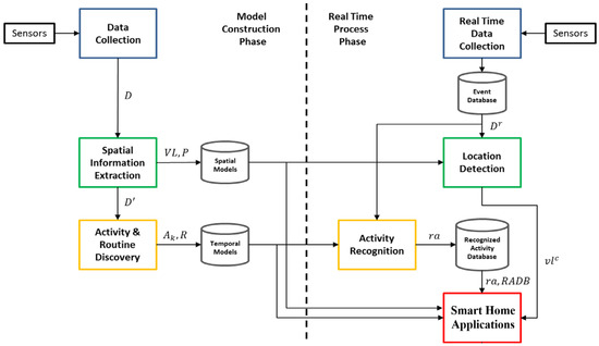
Figure 1. System architecture of the proposed method for smart home applications.

Table 1. Main notations used throughout this study.

Symbol	Description
$d_k$	An event of $d_k=\left(timestamp, sensor ID, sensor status\right)$, $\forall d_k\in D$
$VL$	Virtual location
$V$	A set of vertices representing all sensors
$W$	Symmetric $\left|V\right|\times \left|V\right|$ matrix representing the correlation between each pair of sensors
$E_k$	The event sequence of $k$
$M{E}_k$	The maximal episode of $k$
$F{E}_k$	The frequent episodes of $k$
$Sup\left(f{e}_{k, i}\right)$	The support of the frequent episodes ($f{e}_{k, i}$)
$S_{min}$	The minimal support threshold
$Acc\left(a_{k,i}\right)$	The accuracy of $a_{k,i}$
$A_{min}$	The minimal accuracy threshold
$A{S}_k$	The activity sequence of $k$
$Conf\left(r_k\right)$	The confidence of $r_k$
$CON{F}_{min}$	The minimal confidence threshold

A set of virtual locations is defined as $VL=\left\{v{l}_1,v{l}_2\dots ,v{l}_n\right\}$, where $VL$ denotes a partition of the sensors with the highest modularity, and $v{l}_k$ denotes a set of sensors in a specific virtual location. An event ($e_k=\left\{t_k,i{d}_k,statu{s}_k\right\}$) contains a timestamp ($t_k$), the sensor ID ($i{d}_k$), and the sensor status ($statu{s}_k$) at time $t_k$. A weighted graph ($G=\left(V,W\right)$) is used to model the correlation between sensors in the environment and to discover $VL$. Meanwhile, $W$ is a symmetric matrix representing the correlation between each pair of sensors and is adjusted according to the sensor type of each vertex; the partition of $V$ with the highest modularity is regarded as $VL$. Furthermore, the sensor data ($D$) can be split into $\left\{D_1, D_2\dots , D_n\right\}$ according to the virtual location where sensors are deployed after virtual locations are identified. $D_k$ is transformed into event sequence $E_k$ and split into maximal episode $M{E}_k$ using a sliding window, where $E_k$ denotes the subsequence of $E$ belonging to virtual location $v{l}_k$. Frequent episodes ($F{E}_k$) are discovered from $M{E}_k$, where $Sup\left(f{e}_{k,i}\right)\ge S_{min}$, $\forall f{e}_{k,i}\in F{E}_k$. Activities ($A_k$) are found by analyzing the periodicity of each $f{e}_{k,i}\in F{E}_k$, where $Acc\left(a_{k,i}\right)\ge A_{min}$, $\forall a_{k,i}\in A_k$. Then, $M{E}_k$ is transformed into activity sequence ($A{S}_k$), and routines ($R$) can be discovered from $AS$, where $Conf\left(r_k\right)\ge CON{F}_{min}$, $\forall r_k\in R$. Based on the discovered routines ($VL,\forall A_k,R$), this information can be applied to smart home applications, such as home automation or anomaly detection to identify abnormal behavior of residents or to suggest automation rules that control different aspects of the home environment based on the models constructed from historical sensor data.

In the real-time process phase, real-time sensor data ($D_r$) are collected progressively. As with data collection, $D_r$ is preprocessed, transformed into an event sequence, and stored in the event database. Events stored in the event database are partitioned with a sliding window into maximal episodes. Furthermore, the system recognizes activities from these maximal episodes and stores them in a recognized activity database ($RADB$) if any activity is recognized. In the meantime, the virtual location of the resident ($v{l}^c$) is determined by the virtual location of the last triggered sensor. Finally, after obtaining the virtual location of the resident ($v{l}^c$), the activities that the resident has performed stored in the $RADB$, the discovered activities ($\forall A_k$), and routines ($R$) discovered from the historical sensor data, smart home applications can utilize this information to infer resident behavior of the current virtual location and perform the desired task designed by the application. The details of each component in the system architecture are described in the following sections.

3.1. Data Collection

Data collection is the process that transforms raw sensor data into event sequences. Data collection involves three steps: sensor data collection, data preprocessing, and event extraction.

3.1.1. Sensor Data Collection

Sensors are devices that detect events or changes in the environment and convert them into measurable digital signals. In this study, we use sensors to detect and record the resident’s daily activity in the smart home environment. Thus, sensors are deployed around the environment with unique IDs, and sensor data are sent to the smart home gateway for further analysis. Four types of sensors are used in the proposed method: PIR motion detectors, door contacts, power meters, and binary sensors. A PIR motion detector measures infrared light radiating from objects and generates a record formatted as $\left(timestamp, sensor ID\right)$ when triggered. A door contact is used to sense the opening and closing of doors and generates a record periodically formatted as $\left(timestamp, sensor ID, door status\right)$, $door status\in \left(open, close\right)$. A power meter is used to measure the amount of electric energy consumed by household appliances and generates a record periodically formatted as $\left(timestamp, sensor ID, power\right)$. Finally, binary sensors such as pressure switches, temperature switches, and buttons only have two states: either on or off. The data from the database of the home gateway are raw data. From the home gateway, the data are uploaded periodically to the database in the cloud. All these raw sensor data received by the database in the cloud are analyzed via a data-mining algorithm to generate wellness patterns, which are defined as activities and routines in this study. However, any device or application connected to the Internet is vulnerable to attacks, malware, and tracking software. Maintaining protection for sensors and the system has become a major concern [41]. Therefore, in this study, we adopted and established a chain-of-trust concept to protect data transmission between the home gateway and the cloud. First, a firewall is established to prevent unauthorized or malicious software from accessing the network. A virtual private network (VPN) is utilized to ensure all smart home traffic is transmitted through an encrypted virtual tunnel, and a commercial cloud server is used as the endpoint for traffic originating from the home gateway. We only allow connections via localhost by default and always with TLS, a VPN is utilized to transmit sensor data to the cloud for analysis, and only specific IP addresses are allowed in the environment.

3.1.2. Data Preprocessing

The sensor data collected in the smart home environment might include abnormal data due to sensor malfunction or unexpected environmental inconstancies. As a result, the sensors may produce poor, noisy, and fragmentary data. Thus, to alleviate this situation, sensor data with a status is greater than $\left(mean+standard deviation·3\right)$ or less than $\left(mean-standard deviation·3\right)$ are considered outlier data. Redundant sensor data, outlier data, and incomplete sensor data are be removed. Furthermore, information about the status of sensors, which is not binary, is discretized, such as the status of power meters. For each sensor that needs to be discretized, we apply k-means $\left(K=2\right)$ to partition the statuses into two clusters: $C_{min}$ and $C_{max}$, where $max\left(C_{min}\right)<max\left(C_{max}\right)$. Then, the statuses in $C_{min}$ are transformed into $v^{-}$, and the statuses in $C_{max}$ are changed into $v^{+}$.

To discover virtual locations, the preprocessed data ($D^{\prime }$) and the number of sensors ($n$) are used to extract an event sequence ($E$). They are split into maximal episodes using a sliding window. The event sequence ($E$), time threshold ($TT$), and the weight corresponding to $TT$ ($WT$) are utilized to construct a correlation graph. $TT$ and $WT$ are dynamically determined using the time differences between all sensor events. Then, a weighted graph ($G$) is constructed using the correlations between sensors, and this weight is adjusted according to the sensor type that triggered the event. This weight is stored in a matrix called $IDI$, and both the weighted graph ($G$) and the correlation matrix ($IDI$) are used together with weights $W^m,$ $W^d$, and $\widehat{p}$ in modularity. Sensors are partitioned into virtual locations according to their modularity, and sensors with high modularity are likely to be partitioned into the same virtual location. The procedure of virtual location discovery is illustrated in Figure 2, and details of this procedure are described in the following sections.

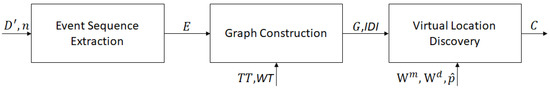
Figure 2. The procedure of virtual location discovery.

3.1.3. Event Extraction

The preprocessed sensor data are transformed into an event sequence ($E$) in the event extraction process. An event represents changing statuses of a sensor, denoted as $\left(t_i,e_i\right)$, where $e_i=\left\{sensor type,sensor ID,status before change,status after change\right\}$ is an event type. For example, given raw sensor data = {(1:05, TV, 0 W), (1:10, TV, 42 W), (1:15, TV, 46 W), (1:22, TV, 0 W)}, we can retrieve the event sequence = {(1:10, TV, TURN ON), (1:22, TV, TURN OFF)}. Algorithm 1 shows the algorithm that extracts event sequences.

Algorithm 1 Event Sequence Extraction.
Input:	$D^{\prime }$: preprocessed sensor data, $n$: number of sensors
Output:	$E$: event sequence
1.	E ← Array() /* Initialize an array to store events */
2.	S ← HashTable (n) /* Initialize a hash table with length 𝑛 to store latest status of sensors */
3.	FOR each d in D′
4.	IF S[d.sensorID] $\ne$ d.st atus
5.	THEN
6.	c ← (S[d.sensorID],d.status) /* Obtain changing status of sensors */
7.	e ← Event(d.timestamp, d.type, d.ID, c) /* Initialize an event */
8.	E.append(e) /* Append the event to E */
9.	S[d.sensorID] = d.status /*Update latest status of the sensor */
10.	ENDIF
11.	ENDFOR
12.	RETURNE

3.2. Implicit Spatial Information Extraction

The main task of this process is to extract implicit spatial information from the event sequence and form the concept of virtual location.

3.2.1. Correlation Graph Construction

A weighted sensor correlation graph ($G=\left(V,W\right)$) is constructed to model the temporal correlations between sensors, where $V$ is a set of vertices representing all the sensors, and $W$ is an asymmetric $\left|V\right|\times \left|V\right|$ matrix representing the correlation between sensors. The higher the correlation between sensors, the greater the similarity between the corresponding vertices. Furthermore, indirect information ($IDI$) is saved in the process of estimating the correlations and stores a set of sensors that are triggered during the time interval between two events. The time correlation between two sensors is calculated based on Equation (1):

$$w\left(v_i,v_j\right)={\displaystyle \sum }_{k=1}^{N_T}{c}_{i,j}^k·w{t}_k$$

(1)

where $w$ is the weight function representing the correlation between the two sensors ($v_i,v_j\in V$), $c_{i,j}^k$ is the time difference between events that are less than the time threshold ($t{t}_k$), and $w{t}_k$ is the weight corresponding to $t{t}_k$. Figure 3 shows an example of how the weight function works.

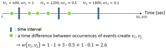
Figure 3. An example of the calculation of the weight function.

A set of time thresholds ($TT$) and a set of weights corresponding to $TT$ ($WT$) are used to increase the weight of the edge between two sensors that are usually triggered together. For example, if a door sensor ($s_k$) is always triggered between sensor $s_i$ and $s_j$, this may imply that the door sensor ($s_k$) is deployed between $s_i$ and $s_j$. This inference can be utilized to decrease the weight between two sensors in different locations. Moreover, sensor placement is unique in each environment, and people tend to have different habits in different environments. Thus, $TT$ and $WT$ in this study are dynamically determined according to the actual environment based on the mean value and the standard deviation of time differences between all sensor events. Algorithm 2 presents the algorithm of correlation graph construction.

Algorithm 2 Correlation Graph Construction.
Input:	$E$: event sequence, $TT$: time thresholds, $WT$: weight corresponding to $TT$
Output:	$G$: weighted graph, $IDI$: matrix stores correlation information of sensor
1.	S ← get_sensor_list(E) /* Iterate through event sequence to obtain sensor list */
2.	LD ← Array(|S|) /* Initiate an array stores each sensors’ time of last occurrence */
3.	TD ← Matrix(|S|, |S|) /* Initiate a matrix stores occurrence time differences between
	𠀃 sensors */
4.	IDI ← Matrix(|S|, |S|) /* Initiate a matrix stores indirect information */
5.	FOR each e∈E
6.	LD[e.ID] ← e.timestamp /* Update last occurrence time of sensor e.ID */
7.	FOR each e∈E, where e.ID≠e.ID
8.	t ← e.timestamp−LD [s.ID] /* Obtain the time difference */
9.	𝑇𝐷[𝑠.𝐼𝐷,𝑒.𝐼𝐷].append(𝑡) /* Append time difference to 𝑇𝐷 */
10.	𝑖𝑠𝑑←get_indirect_sensor_list(𝑒.𝑡𝑖𝑚𝑒𝑠𝑡𝑎𝑚𝑝,𝐿𝐷[𝑠.𝐼𝐷]): /* Obtain sensors occurred
	between 𝑒.𝑡𝑖𝑚𝑒𝑠𝑡𝑎𝑚𝑝 and
	𝐿𝐷[𝑠.𝐼𝐷] */
11.	FOR each 𝑠′∈𝑖𝑠𝑑
12.	𝐼𝐷𝐼[𝑠.𝐼𝐷,𝑒.𝐼𝐷].append(𝑠′) /* Store the sensors to 𝐼𝐷𝐼 */
13.	ENDFOR
14.	ENDFOR
15.	ENDFOR
16.	Create an undirected weighted graph 𝐺 with |𝑆| vertices
17.	FOR each 𝑠𝑖,𝑠𝑗∈𝑆, where 𝑖<𝑗
18.	𝑤←0 /* Initial an integer to store the sum of weight */
19.	FOR each 𝑡∈TD[𝑠𝑖.𝐼𝐷,𝑠𝑗.𝐼𝐷] or TD[𝑠𝑗.𝐼𝐷,𝑠𝑖.𝐼𝐷]
20.	FOR each 𝑡𝑡𝑘∈𝑇𝑇 /* Iterate through 𝑇𝑇, 𝑡𝑡𝑘∈𝑇𝑇 is in ascending order */
21.	IF 𝑡<𝑡𝑡𝑘
22.	THEN
23.	𝑤=𝑤+𝑤𝑡𝑘 /* Add the weight according to the time difference */
24.	ENDIF
25.	ENDFOR
26.	ENDFOR
27.	Add an edge between 𝑠𝑖 and 𝑠𝑗 with weight 𝑤
28.	ENDFOR
29.	RETURN 𝐺,𝐼𝐷𝐼 /*Return the weighted graph and matrix storing indirect information */

3.2.2. Virtual Location Discovery

Sensors in the environment are partitioned into clusters based on the sensor correlation graph and form the concept of virtual locations, denoted as $v{l}_k\in VL$. However, this process does not attempt to match actual rooms with virtual locations, instead grouping sensors that are physically close to each other or that have strong correlations with other sensors within a set period [42]. Thus, a large space may form more than one virtual location if sensors are deployed far from each other or are not often triggered in correlation with other sensors. Let $C=\left\{C_1,\dots ,C_k\right\}$ be a partition of $V$, where $C_1\cup \dots \cup C_k=V$ and $C_i\cap C_j=\varnothing \forall i\ne j$. The modularity used to measure the quality of the partition expressed in Equation (2).

$$Q=\frac{1}{2m}{\displaystyle \sum }_{ij}\left[W_{ij}-\frac{s{w}_{i}s{w}_j}{2m}\right]\delta \left(c_i,c_j\right)$$

(2)

where $W_{ij}$ represents the edge weight between vertices $v_i$ and $v_j$; $s{w}_i$ and $s{w}_j$ represent the sum of edge weights connected to vertices $v_i$ and $v_j$, respectively; $m$ represents the sum of all edge weights in the graph; $\frac{s{w}_{i}s{w}_j}{2m}$ represents the probability of the existence of an edge between vertices $v_i$ and $v_j$ if the edges were randomly connected; and $\delta \left(c_i,c_j\right)$ returns 1 if vertices $v_i$ and $v_j$ are in the same cluster and returns 0 otherwise. Modularity represents the fraction of the edges in a given virtual location subtracted from the expected fraction if edges were randomly connected, and its value is in the range $\left[-\frac{1}{2},1\right)=\left\{Q|-\frac{1}{2}\le Q<1\right\}$.

Modularity was designed to measure the quality of the clusters. Thus, clusters with higher modularity imply that sensors are strongly correlated with sensors in the same virtual location. In contrast, sensors with weaker correlations are partitioned into different clusters. Hence, virtual location discovery can be formulated as a modularity optimization problem to find clusters with maximized modularity. Furthermore, there are cases in which sensors may have a strong correlation and are physically deployed near each other but separated by walls. As a result, it is sometimes difficult to distinguish which event occurred in which room. To alleviate this phenomenon, different characteristics of sensors, such as motion detectors and door sensors, can be utilized to improve clustering results. For example, a motion detector event can represent the presence of a resident, but a binary sensor will not be triggered when a resident walks past it. Thus, the correlation between a sensor and a motion detector may be more important than a binary sensor. Moreover, suppose a door sensor is always triggered between two subsequent events generated by the other two sensors. This situation implies that these two sensors are located in different regions of the environment. Based on this principle, the weights of the sensor correlation graph ($G$) may be adjusted according to the type of sensor that triggers the event. The adjustment rule can be formulated as follows: increase the weight between a motion detector and any subsequent sensors triggered after the motion detector and decrease the weight between two sensors that always have a door sensor triggered between them. The virtual location discovery algorithm extends the Louvain method [36] to discover virtual locations, as illustrated in Algorithm 3. The extension was made to adjust the weight of each edge according to sensor type, and door sensors are not situated in any virtual location act as a bridge between locations. This algorithm represents an attempt to improve modularity by removing a sensor from its virtual location and moving it to a neighboring virtual location until increasing modularity becomes impossible.

Algorithm 3 Virtual Location Discovery.
Input:	$G$: weighted graph, $IDI$: matrix stores correlation information of sensor, $W^m$: weight to increase the edge between a sensor and a motion sensor, $W^d$: weight to decrease the edge between sensors which are split by a door sensor, $\widehat{p}$: minimal proportion of time differences between a door sensor
Output:	$C$: partition with the highest modularity
1.	FOR each node $v_i,v_j\in V$, where $\mathrm{i}<\mathrm{j}$
2.	IF $v_i.type=motion$ or $v_j.type=motion$
3.	THEN
4.	$w_{i,j}=w_{i,j}·W^m$ /* Increase $w_{i,j}$ weight up to $W^m$-fold */
5.	ENDIF
6.	FOR each node $v_k$, where $v_k.type=door,k\ne i,k\ne j$
7.	IF proportion of $v_k$ in $CIL\left[v_i.ID,v_j.ID\right]>\widehat{p}$
8.	THEN
9.	$w_{i,j}=w_{i,j}·W^d$ /* Decrease $w_{i,j}$ weight down to $W^d$-fold */
10.	ENDIF
11.	ENDFOR
12.	ENDFOR
13.	$C\leftarrow$ Assign each node of $G$ to its own virtual location;
14.	REPEAT
15.	FOR each node $v_i$
16.	$increase\leftarrow 0$; /*Initial an integer to store the increasing modularity */
17.	FOR each neighbor $v_j$ of $v_i$
18.	$t\leftarrow$ modularity_gain ($v_i$, $v_i$); /* Compute changes in modularity after remove
	$v_i$ from its own virtual location and move it to
	virtual location $v_j$ */
19.	IF $t>increase$
20.	THEN
21.	$\mathrm{increase}\leftarrow \mathrm{t}$; /* Update $increase$ if $t$ is greater than itself */
22.	ENDIF
23.	IF $increase\ne 0$
24.	THEN
25.	$C\leftarrow$ remove $v_i$ from its own virtual location and move it to the virtual location of $v_j$
26.	with highest $increase$;
27.	ELSE
28.	Exit the loop;
29.	ENDIF
30.	ENDFOR
31.	ENDFOR
32.	UNTIL
33.	RETURN$C$

3.2.3. Probability Matrix Construction

After the virtual locations are discovered, the location of each sensor is known. When a sensor ($s_k$) is triggered at time $t_k$, resident occupancy can be inferred at $t_k$ in the virtual location of $s_k$. A probability matrix ($P$) can be constructed after dividing 24 h of a day into time slots ($TS$) with equal size. $P$ is a $\left|VL\right|\times \left|TS\right|$ matrix, where $VL$ is a set containing all virtual locations, $TS$ is a set containing all time slots, and $P$[$v{l}_k$, $t{s}_k$] represents the probability of user occupancy during time slot $t{s}_k$ and in virtual location $v{l}_k$ based on historical data. The concept of the probability matrix is shown in Figure 4.

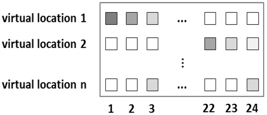
Figure 4. Concept of the probability matrix; darker colors represent higher probability.

3.3. Activity and Routine Discovery

In this study, we use an activity to describe a resident’s periodic behavior. Discovery of the activities in each virtual location and the association rules between them involves four steps, namely event sequence segmentation, frequent episode mining, periodicity analysis, and routine discovery. Although each resident may have specific behavioral habits, it is not easy to discover and mine these patterns because considerable randomness in activities and irregular or inconsistent activities may occur in daily living. The next activity is decided by the current activity and previous activities. Any changes may break the periodic nature of an activity. Thus, discovering the activities in each virtual location first, then mining their routines using transitional probability between activities, may alleviate this problem by allocating activities to a location and inferring routines according to different activity combinations and probabilities between activity transitions. In addition, allowing limited deviations from periodic behavioral routines may facilitate the formation of daily activities and routines. As a result, the discovered patterns are more compact than those without the knowledge of sensor location, which means the number of discovered patterns is significantly reduced with the help of the virtual locations. This is because not knowing the location where activities occur makes it impossible to distinguish where the activity happened and makes it difficult to provide an accurate boundary when attempting to discriminate the start and end of a behavior.

Furthermore, a similar pattern with slight deviation will create a significant amount of behavioral activities. This may distract the recommendation decisions made by smart home applications. Figure 5 shows the concept of differences between activity and routine discovery methods with and without the concept of virtual location.

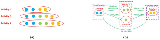
Figure 5. Concept of the differences in activities between activity and routine discovery methods (a) without virtual location and routine and (b) with virtual location and routine.

To achieve this, the entropy rate [43] is utilized for similarity measures and to detect the degree of deviation between the sequence of periodic behavioral routines and the activities and routines performed by the resident. Entropy usually serves as a measure of the randomness of a sequence [44]. Thus, it can be applied to the activity and routine sequences performed by the resident, leveraging the already constructed probability matrix ($P$) [45]. The similarity measure is calculated based on Equation (3):

$$\epsilon =-{\displaystyle \sum }_{i,j}{P}_{ij}\times \log \left(P_{ij}\right)$$

(3)

where $\epsilon$ is the entropy value, and $P_{ij}$ is the transitional probability between activities $A_i$ and $A_j$ from activity sequence $A{S}_k$. Lower entropy values indicate a greater probability that activity $A_j$ occurred after activity $A_i$, and higher entropy values indicate a lower probability. However, it may be insufficient to only consider the transitional probabilities between activities in periodic behavioral routines; the duration of each activity should also be considered to reduce the potential false-positive rate in order improve accuracy when determining whether current activities deviate from periodic behavior routines performed by the resident, i.e., by averaging the duration of each activity and dividing it by the number of times it has occurred. The average duration of an activity is calculated based on Equation (4):

$$avg\left(A_i\right)=\frac{{{\displaystyle \sum }}_{j=1}^{m}t\left(A_i,k\right)}{m},m=count\left(A_i\right)$$

(4)

where $t\left(A_i,k\right)$ represents the duration of the $k$th occurrence of activity $A_i$, and $m$ is the total number of times that activity $i$ has occurred. Here, cosine similarity is utilized to quantify the similarity relation between the activities and routines performed by the resident and the activities in the periodic behavioral routines considering activity durations. The cosine similarity is calculated based on Equation (5):

$$S_d^{R_d}=\cos \left(d,R_d\right)=\frac{{{\displaystyle \sum }}_{i=1}^{n}t\left(d\left(A_i\right)\right)\times t\left(b\left(A_i\right)\right)}{\sqrt{{{\displaystyle \sum }}_{i=1}^{n}t{\left(b\left(A_i\right)\right)}^2}\times \sqrt{{{\displaystyle \sum }}_{i=1}^{n}t{\left(d\left(A_i\right)\right)}^2}}$$

(5)

where $S_d^{R_d}$ represents the similarity relation between the activities and routines, $R_d$ is the periodic behavioral routines of the same day of the week for which the sequence of activities is being analyzed, $d$ is the day for which the sequence of activities is analyzed, $i$ is equal to hours, $0<i\le 24$, $t\left(d\left(A_i\right)\right)$ is the duration of activity $A_i$ on the day being evaluated, and $t\left(b\left(A_i\right)\right)$ is the duration of activity $A_i$ in the periodic behavioral routines. A cosine similarity between two vectors close to 1 implies that the activities and routines performed by the resident and the activities in the periodic behavioral routines are similar. A cosine similarity is close to 0 indicates fewer similarities between them. Thus, by comparing the similarity between periodic behavior routines and the activities and routines performed by the resident, knowledge can be obtained about whether the resident has deviated from their periodic behavioral routines.

3.3.1. Event Sequence Segmentation

A sliding window with two parameters ($T_{EP}$ and $C_{EP}$) is used to partition the event sequence ($E_k$) in each virtual location ($v{l}_k$) into overlapping maximal episodes. A maximal episode is an episode meeting the two constraints: $T_{EP}$ and $C_{EP}$, where $T_{EP}$ is the maximal time difference between events in an occurrence of an episode, and $C_{EP}$ is the maximal capacity of an episode. In event sequence segmentation, the events in $E_k$ are split into maximal episodes from $E_k$. A sliding window collects the events and generates an episode when the constraints are exceeded. If $T_{EP}=\infty$, then $E_k$ is split into maximal episodes with size $C_{EP}$. If $C_{EP}=\infty$, then $E_k$ is split only depending on the time difference. Figure 6 shows an example of the procedure of event sequence segmentation.

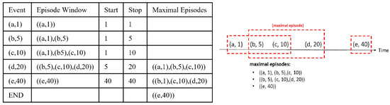
Figure 6. Example of event sequence segmentation.

3.3.2. Frequent Episode Mining

The problem of mining frequent episodes in maximal episodes is similar to the problem of mining frequent item sets in a list of transactions. One of the main differences between these two problems is that the maximal episodes are overlapped, so the number of occurrences of an episode counted in maximal episodes is greater than the actual number of occurrences of this episode.

This study extends the split and merge algorithm (SaM) to discover frequent episodes as shown in Algorithm 4. SaM is a frequent itemset mining algorithm proposed in [46]. The advantages of SaM are its simplicity of data structure and the convenience of running on external storage. The following change is made: instead of using an integer to represent the support of an event, we use an additional list called $t\_list$, which stores timestamps of occurrences of the event. Therefore, the actual support of the event is the number of distinct timestamps in the list as shown in Algorithm 5. For example, if an event sequence ($\left\{\left(a,1\right),\left(b,8\right),\left(c,9\right),\left(d,14\right)\right\}$) is partitioned into two maximal episodes ($\left\{\left(a,1\right),\left(b,8\right),\left(c,9\right)\right\}$, $\left\{\left(b,8\right),\left(c,9\right),\left(d,14\right)\right\}$) with $T_{EP}$ = 10, the number of occurrences of episode $\left\{b,c\right\}$ in maximal episodes is two, but the actual number of occurrences of $\left\{b,c\right\}$ can be acquired by counting the number of distinct timestamps in $t_{list}=\left\{\left(8,9\right),\left(8,9\right)\right\}$, which is one in this case. Figures 10 and 11 show the algorithms of frequent episode mining.

Algorithm 4 Frequent Episode Discovery.
Input:	$E_k$: event sequence in virtual location $v{l}_k$, $M{E}_k$: maximal episodes in virtual location $v{l}_k$, $S_{min}$: minimal support
Output:	$F{E}_k$: frequent episodes in virtual location $v{l}_k$
1.	Count the number of occurrences of each event type in $E_k$
2.	Remove the duplicate event types in each $ME$
3.	Sort the event types in each $ME$ by their count
4.	Sort the $ME$ by the count of their first event type
5.	Initialize set of $F{E}_k=\left\{\right\}$
6.	$n$← $ESaM(M{E}_k, \{\}, S_{min},F{E}_k)$
7.	RETURN $F{E}_k$

Algorithm 5 Extended Split and Merge Algorithm.
Input:	$ME$: maximal episodes, $P$: prefix episode, $S_{min}$: minimal support, $FE$: frequent episodes
Output:	$n$: the number of frequent episodes
1.	Initialize event type $i$, /* leading event type */
2.	integer $n$, /* the number of frequent episodes */
3.	List of timestamp $s$, /* $t\_list$ store the timestamps */
4.	List of maximal episode $b$, /* store the split result */
5.	List of maximal episode $c$, /* store the split result */
6.	List of maximal episode $d$ /* store the output */
7.	𝑛←0
8.	WHILE $ME$ is not empty
9.	$b$←[ ] /* initialize the split result */
10.	$s$←[ ] /* initialize $t_{list}$ */
11.	$i$←$ME\left[0\right].\mathrm{events}\left[0\right].\mathrm{type}$ /* get the leading event type of the first maximal episode */
12.	WHILE $ME$ is not empty and $ME\left[0\right].\mathrm{events}\left[0\right].\mathrm{type}=i$ // split data based on this item
13.	Append $ME\left[0\right].\mathrm{events}\left[0\right].\mathrm{timestamp}$ to $s$
14.	Remove $ME\left[0\right].\mathrm{events}\left[0\right]$ from $ME\left[0\right].\mathrm{events}$
15.	ENDWHILE
16.	IF $ME\left[0\right].\mathrm{events}$ is not empty
17.	THEN
18.	Remove $ME\left[0\right]$ from $ME$ and append it to $b$
19.	ELSE
20.	Remove $ME\left[0\right]$ from $ME$
21.	ENDIF
22.	$c$←$b$ /* store the split result */
23.	$d$←[ ] /* initialize the merge result */
24.	WHILE $ME$ and $b$ are both not empty do /* merge data */
25.	IF $ME\left[0\right].\mathrm{events}>b\left[0\right].\mathrm{events}$
26.	THEN
27.	Remove $ME\left[0\right]$ from $ME$ and append it to $d$
28.	ELSE IF $ME\left[0\right].\mathrm{events}<b\left[0\right].\mathrm{events}$
29.	THEN
30.	Remove $b\left[0\right]$ from $b$ and append it to $d$
31.	ELSE
32.	$b\left[0\right].\mathrm{support}=b\left[0\right] .\mathrm{support}+ME\left[0\right].\mathrm{support}$ +
33.	Remove $b\left[0\right]$ from $b$ and append it to $d$
34.	Remove $ME\left[0\right]$ from $ME$
35.	ENDIF
36.	ENDWHILE
37.	WHILE $ME$ is not empty
38.	Remove $ME\left[0\right]$ from $ME$ and append it to $d$
39.	ENDWHILE
40.	WHILE 𝑏 is not empty
41.	Remove $b\left[0\right]$ from 𝑏 and append it to $d$
42.	ENDWHILE
43.	$ME$←$d$
44.	IF the number of distinct timestamps in $\mathrm{s}\ge s_{min}$ /* if the split event is frequent */
45.	THEN
46.	$P$←$\mathrm{P}\cup \left\{i\right\}$
47.	Append $P$ with $s$ to $FE$
48.	$n$←$n+1+\mathrm{ESAM}\left(c, P, s_{min}, FE\right)$
49.	$P$←$P-\left\{i\right\}$
50.	ENDIF
51.	ENDWHILE
52.	RETURN 𝑛 /*return the number of frequent episodes */>

3.3.3. Periodicity Analysis

Gaussian distribution describes the time distribution of the occurrences of each frequent episode. A frequent episode with an accuracy that corresponds to the given Gaussian distribution and is greater than the minimal accuracy ($AC{C}_{min}$) is regarded as an activity. For each frequent episode, time intervals are derived from the timestamps of their occurrences with maximal standard deviation ($S{D}_{max}$) and period ($\pi$). An interval consists of timestamps for which the time difference between every two adjacent timestamps in this interval is less than $S{D}_{max}$. The concept of finding the intervals is shown in Figure 7. According to the length of the dataset, different periods are tested: 24 h, 7 days, etc.

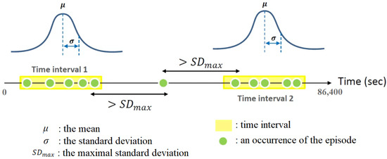
Figure 7. The concept of finding the intervals.

For each interval of each frequent episode, the parameters of the Gaussian distribution that best describe the interval are estimated. The maximum likelihood method is the standard approach to this problem and requires the maximization of the log-likelihood function. In this study, we use existing and well-developed tools to solve this problem. After two parameters, the mean and the standard deviation $\left(\mu ,\sigma \right)$ of the Gaussian distribution are estimated, the accuracy of each frequent episode can be calculated, which is the number of occurrences within the time interval $(\mu -2·\sigma$, $\mu +2·\sigma$). Every interval with a corresponding accuracy greater than $A_{min}$ for each frequent episode forms an activity.

3.3.4. Routine Discovery

A routine ($r_i$) is an extended association rule with confidence greater than the minimal confidence ($CON{F}_{min}$) used to describe the temporal relation between activities. After the activities are discovered, the event sequence ($E_k$) in each virtual location ($v{l}_k$) is transformed into the activities sequence ($A{S}_k$), where $A{S}_k$ is a sequence of the occurrences of the activities recognized from $E_k$. Collect all $A{S}_k$ into $AS$ and sort $AS$ by their timestamps. Sequentially iterate through the sorted $AS$ and store each time difference into the matrix $TD$, where $TD$[$a_i$, $a_j$] stores time differences between each occurrence of $a_i$ and $a_j$. For each $a_i$ and $a_j$, where $i\ne j$, if the standard deviation of time differences in $TD$[$a_i$, $a_j$] is less than $S{D}_{max}$ and the confidence is greater than the minimal confidence ($CON{F}_{min}$), a routine ($r_i=(a_i$, $a_j$, $mean$, $std$, $conf$)) is generated, where $mean$ is the mean value of the time difference in $TD$[$a_i$, $a_j$], $std$ is the standard deviation of the time differences in $TD$[$a_i$, $a_j$], and $conf$ is the ratio of the number of time differences in $TD$[$a_i$, $a_j$] to the number of occurrences of $a_i$.

4. Experiment and Discussion

In this section, an experiment was designed and conducted to explore the effectiveness of the proposed virtual location-based periodic behavioral routine discovery process and assess the feasibility of a practical application. Thus, the proposed method is evaluated on three smart home datasets: the Kasteren dataset [47], the Aruba dataset [48], and our self-collected dataset. The details of these datasets are depicted in Table 2.

Table 2. Details of datasets.

	KA	KB	KC	Aruba	Our Dataset
Age	26	28	57	Elderly	24
Gender	Male	Male	Male	Female	Male
Rooms	3	2	6	7	4
Duration	25 days	27 days	20 days	220 days	32 days
Sensors	14	23	21	34	13
Activities	10	13	16	10	Unannotated
No. of Events	2458	38,150	45,400	1,602,912	57,935

Wireless sensor networks are used to observe residents’ behavior in their homes. Each dataset utilizes different types of sensors; for instance, the Kasteren dataset uses reed switches, mercury contacts, PIR motion detectors, pressure mats, and float sensors; the Aruba dataset utilizes PIR motion detectors, temperature, and door sensors in their experiment; and our dataset uses PIR motion detectors, magnetic door contact switches, and power meter switches. The experiments on all datasets are conducted without predefined sensor locations. House floor plans indicating the locations of the sensors are shown in Figure 8, Figure 9 and Figure 10. The virtual location-based periodic behavioral routine discovery process described in Section 3 is applied to all datasets in four situations: (1) discover the virtual locations without adjusting the weights, (2) discover the virtual locations considering the door sensors, (3) discover the virtual locations considering the motion detectors, and (4) discover the virtual locations considering both the door sensors and the motion detectors.

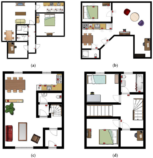
Figure 8. Floor plans of Kasteren houses; red boxes represent the sensors [47]. (a) House A. (b) House B. (c) House C, first floor. (d) House C, second floor.

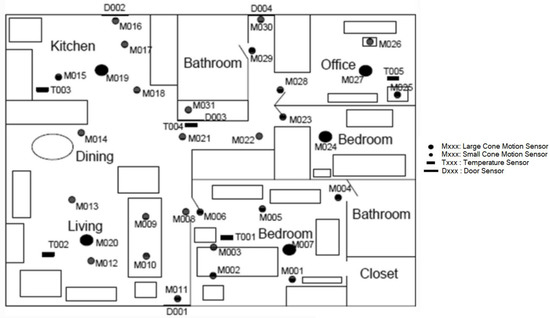
Figure 9. The floor plan of the Aruba dataset [48].

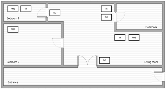
Figure 10. The floor plan of our dataset.

4.1. Experimental Setup

The parameters used in the proposed method are described in detail in Table 3.

Table 3. Overview of the parameters of the proposed method.

Name	Value Range	Recommended Value
$\widehat{p}$	0–100%	60%
$W^m$	$\ge$1.0	2
$W^d$	$\ge$0.0	0.25
$T_{ep}$	0–24 h	30 min
$C_{ep}$	$\ge$1.0	$\infty$
$S_{min}$	0–100%	40%
$S{D}_{max}$	0–24 h	1 h
$AC{C}_{min}$	0–100%	40%
$CON{F}_{min}$	0–100%	40%
$\epsilon$	$\ge$1.0	2
$P{A}_{min}$	0–100%	20%
$P{A}_{max}$	0–100%	80%
$AL$	0–100%	60%

4.2. Evaluation Metrics

In the experiments, we employed widely used metrics, namely homogeneity, completeness, and V-measure, to evaluate the performance of different models in clustering and classification. Because we know the actual location of each sensor, we can use V-measure to evaluate the results of virtual location discovery. The authors of [49] defined homogeneity and completeness as objectives for any clustering result; homogeneity is used to check whether all of the clusters only contain members with a single label, and completeness checks whether every member of a given label is assigned to the same cluster. Furthermore, the best homogeneity scores are always at the bottom of the dendrogram, and completeness favors large clusters and decreases the score if members of the same class are divided into different clusters. Therefore, the top of the dendrogram, where all the sensors reside in a single cluster, always achieves the maximum completeness score. V-measure is computed as the harmonic mean of the homogeneity and completeness scores and is designed to balance them. A high V-measure is achieved by making a cluster with high homogeneity and completeness. The value of all three metrics is between zero and one, where one is the maximum score and vice-versa. These metrics determine how close a given clustering is to its ideal definition by examining the conditional entropy of the class distribution given the proposed clustering. Homogeneity is defined as follows.

$$H\left(C|K\right)=-{\displaystyle \sum }_{k=1}^{\left|K\right|}{\displaystyle \sum }_{c=1}^{\left|C\right|}\frac{a_{ck}}{N}log\frac{a_{ck}}{{{\displaystyle \sum }}_{c=1}^{\left|C\right|}{a}_{ck}}$$

(6)

$$H\left(C\right)=-{\displaystyle \sum }_{c=1}^{\left|C\right|}\frac{a_{ck}}{N}log\frac{{{\displaystyle \sum }}_{k=1}^{\left|K\right|}{a}_{ck}}{n}$$

(7)

where $C$ is a set of classes ($C_{i_{1..n}}$), $K$ is a set of clusters ($K_{j_{1..m}}$), $a_{ck}$ represents a member of class $c$ that the element of cluster $k$, and $N$ is the number of the data points. Based on Equations (6) and (7), homogeneity is calculated according to Equation (8):

$$h=\left\{\begin{array}{c}if H\left(C|K\right)=0 then h=1 \\ else h=1-\frac{H\left(C|K\right)}{H\left(C\right)} \end{array}\right.$$

(8)

Completeness is symmetrical to homogeneity. Therefore, completeness can be calculated based on Equation (9):

$$c=\left\{\begin{array}{c}if H\left(K|C\right)=0 then c=1 \\ else c=1-\frac{H\left(K|C\right)}{H\left(K\right)} \end{array}\right.$$

(9)

As mentioned previously, V-measure is calculated with the harmonic mean of homogeneity and completeness. Thus, the V-measure can be calculated based on Equation (10):

$$V_{Measure}=\frac{\left(1+\beta \right)\times h\times c}{\left(\beta \times h\right)+c}$$

(10)

By assuming $\beta$ is equal to 1, V-measure can be calculated as follows.

$$V_{Measure}=\frac{2\times h\times c}{h+c}$$

(11)

4.3. Experimental Result

4.3.1. Experiments for Virtual Location Discovery

Table 4 shows the scores of virtual location discovery applied to four scenarios presented in three datasets. The KA dataset has two actual rooms: the toilet and the kitchen. Before adjusting the weights of $G$, the washing machine in the kitchen and the toilet flush were in the same cluster. The possible causes include that the use of the washing machine is not likely during dining time. After considering the door contact, the toilet flush was in a cluster alone, and the sensors in the kitchen were in the same cluster. The KB dataset has three actual rooms: kitchen, toilet, and bedroom. Before adjusting the weights of $G$, the toilet flush and the sensors in the kitchen were in two different clusters. After considering the door contact, the toilet flush was in a cluster alone, but the sensors in the kitchen were still in two different clusters. After considering both door contacts and motion detectors, the sensors in the kitchen were in the same cluster. The KC dataset has five actual rooms, namely the kitchen, living room, and toilet on the first floor and the bathroom and bedroom on the second floor. Before adjusting the weights of $G$, the sensors on the first floor and the bed pressure mat on the second floor were in the same cluster, and the rest of the sensors on the second floor were in the same cluster. After considering the door contact, the sensors on the first floor were in the same cluster, and the sensors on the second floor were in the same cluster. The possible causes include the sensors in the bedroom having a significant correlation with the sensors in the bathroom. Although the weights between the bedroom and the bathroom sensors were decreased, the sensors in the same room were still not partitioned into the same cluster. After considering both door contacts and motion detectors, the sensors in the bedroom were in the same cluster, as were the sensors in the bathroom. Because there is no door contact or actual boundary around the living room, the couch and the sensors in the kitchen were in the same cluster.

Table 4. Scores of virtual location discovery in each dataset.

	Dataset	Origin	Door	Motion	Door/Motion
Homogeneity	KA	0.57	1.00	N/A	N/A
	KB	0.45	0.75	0.68	1.00
	KC	0.39	0.58	0.69	0.81
	Aruba	0.70	N/A	0.70	N/A
	Ours	0.14	0.69	0.37	0.69
Completeness	KA	0.37	1.00	N/A	N/A
	KB	0.60	0.71	1.00	1.00
	KC	0.78	1.00	0.86	1.00
	Aruba	0.95	N/A	0.95	N/A
	Ours	0.21	1.00	0.54	1.00
V-measure	KA	0.45	1.00	N/A	N/A
	KB	0.51	0.73	0.81	1.00
	KC	0.52	0.73	0.77	0.90
	Aruba	0.81	N/A	0.81	N/A
	Ours	0.17	0.81	0.44	0.81

N/A denotes this type of sensor in not available in the evaluation.

The Aruba dataset has seven actual rooms: two bathrooms, two bedrooms, an office, and a kitchen, with the dining and the living room in the same space. Most sensors are motion detectors, and door contacts were not deployed between rooms. Thus, the score of clusters does not increase even after adjusting the weights of $G$. The sensors in the bathroom, office, and bedroom were in the same cluster, and the kitchen, dining room, and living room sensors were partitioned into two clusters. Our dataset has four actual locations: the first bedroom, the second bedroom, the living room, and the kitchen. Before adjusting the weights of $G$, the motion detector in the living room, the motion detection in the kitchen, and the appliance in the first bedroom were in the same cluster, and the rest of the sensors were in the same cluster. After considering the door contact, the second bedroom’s motion detector and the living room sensors were in the same cluster, and the rest of the sensors were in the same cluster. After considering the motion detector, the appliances in the first bedroom were in the same cluster, and the rest of the sensors were in the same cluster. Because there is no sensor between the second bedroom and the living room, the score did not improve after considering both door contacts and motion detectors.

The virtual location is an abstract location that may not be consistent with the actual site. The experiments revealed that the following factors might affect the result of virtual location and cause differences between them:

• The number of sensor usages: a sensor may be misclassified if the value is low;
• The number of sensors: a sensor may be easily misclassified as the neighbor’s location if it is the only sensor in its location;
• The boundary between locations: it is difficult to distinguish between two locations that are close to each other.

Misclassifying a sensor to a location that it does not belong to may cause the following consequences:

• The discovered activities may lack events created by the misclassified sensors;
• An activity consisting of many events may be split into many activities consisting of fewer events;
• The virtual location of the user might be determined incorrectly.

However, the differences between virtual and actual locations may be reduced as more data are collected. The experimental results show that even in the above situations, 81% accuracy is still achieved.

4.3.2. Experiments for Activity Discovery

The activity discovery process described in Section 3.3 is applied to all datasets in two situations: (1) discover activities from all sensors and (2) discover activities from each virtual location. First, to demonstrate the effect of virtual location in the activity discovery process, we perform activity discovery with and without utilizing virtual location, as illustrated in Table 5 and Table 6. Based on the annotation and time distribution of each activity, we can compare discovered activities performed by the resident with annotated activities. In Table 5, KA’s first activity is “going to bed”, and the second activity describes the periodic behavior as “using the toilet”. Moreover, the third activity is “leaving the house”. In KB, the first activity is “leaving the house”, the second is “preparing brunch”, and the third activity is “taking a shower”. In KC, the first activity is “going to bed”, the second activity is “using the toilet”, and the third activity is “preparing dinner”. Lastly, the first activity in Aruba is “going to bed”, the second activity is “meal preparation”, and the third activity is “work”.

Table 5. Results of activity discovery in each dataset without virtual location.

Dataset	Activity Discovered without VL	Accuracy
KA	Hall-Bedroom door OFF, Hall-Bedroom door ON	84%
	Hall-Toilet door ON, ToiletFlush ON, ToiletFlush OFF, Hall-Toilet door OFF, Hall-Bedroom door ON	84%
	Frontdoor OFF, Frontdoor ON	84%
KB	PIR keuken ON, frontdoor OFF, frontdoor ON, PIR keuken OFF	74%
	frontdoor OFF, PIR keuken ON, frontdoor ON, PIR kachel ON, PIR kachel OFF, PIR keuken OFF	58%
	temp shower OFF, temp shower ON, toilet door OFF, toilet door ON, PIR keuken ON	55%
KC	deur slaapkamer OFF, mat bed rechts, drukmat OFF, deur slaapkamer ON, mat bed rechts, drukmat ON	89%
	deur slaapkamer OFF, badkamer klapdeur links OFF, badkamer klapdeur links ON	86%
	voordeur, reed OFF, voordeur, reed ON, mat bank, huiskamer OFF, mat bank, huiskamer ON	84%
Aruba	M021 ON, M008 ON, M006 ON, M003 ON, M002 ON	93%
	M013 ON, M014 ON, M019 ON, M015 ON, M019 ON	89%
	M029 ON, M028 ON, M027 ON, M026 ON, M027 ON	88%

Table 6. Results of activity discovery in each dataset with virtual location.

Dataset	VL No.	Activity Discovered with VL	Accuracy
KA	0	Hall-Bedroom door OFF, Hall-Bedroom door ON	84%
	1	Hall-Toilet door ON, Hall-Toilet door OFF, ToiletFlush ON, ToiletFlush OFF	89.50%
	2	Frontdoor ON, Frontdoor OFF	84%
KB	0	frontdoor ON, frontdoor OFF	74%
	1	PIR keuken ON, PIR kachel ON, PIR kachel OFF, PIR keuken OFF	72.20%
	2	toilet door door ON, temp shower ON, temp shower OFF, toilet door door OFF	67.50%
KC	1	deur slaapkamer OFF, mat bed rechts, drukmat OFF, deur slaapkamer ON, mat bed rechts, drukmat ON	89%
	2	badkamer klapdeur links OFF, badkamer klapdeur links ON	94%
	3	voordeur, reed OFF, voordeur, reed ON, mat bank, huiskamer OFF	90%
Aruba	2	M008 ON, M006 ON, M003 ON, M002 ON	95%
	1	M014 ON, M019 ON, M015 ON, M019 ON	93%
	0	M027 ON, M026 ON, M027 ON	90%

By comparing the discovered activities between Table 5 and Table 6, we can see that by assigning activities to virtual locations according to the correlation between sensors and triggered sensor types, events that occurred not within the same location are not discovered as an activity in that virtual location. This not only separates events that occurred in a different location, but a more accurate periodic behavior of the resident can be obtained to help determine the resident action or status. For example, in KA in Table 5, the second activity, “using the toilet”, contains “hall-bedroom door ON”, and the same activity discovered by utilizing the virtual location shown in KA of Table 6 does not. This is because “hall-bedroom door” is assigned to virtual location 0, and both “Hall-Toilet door” and “ToiletFlush” are assigned to virtual location 1. The third activity, “taking a shower”, in KB in Table 5 appears to contain “PIR keuken (kitchen) ON”, and the same discovered activity shown in KB in Table 6 also separated “keuken (kitchen)” from “temp shower” and “toilet door” into different virtual location. The same phenomenon can also be observed in KC in Table 6. As we can see, assigned sensors in virtual locations can increase the accuracy of discovered activities. However, only motion and temperature sensors were installed inside the environment in the Aruba dataset. Door sensors are only placed at different entrances to the environment, not between rooms. Thus, events that occur in the environment contain mostly the trajectory of the resident. The disadvantage of this can be seen in the results of Aruba in Table 6. The first activity, “going to bed”, still contains the sensor event “M008”, which occurred in the hallway just outside the bedroom, and the second activity, “meal preparation” cannot be distinguished from sensor events that occurred in the dining room, which is close to the entrance of the kitchen. However, the proposed method excluded sensor event “M021”, which occurred at the end of the hallway, as well as “M013” in the living room, from the activity discovery process. By doing so, the activity discovery accuracy for Aruba was slightly increased, as shown in Table 6.

To further examine the effectiveness of the proposed method, we evaluated the computational time, the number of activities, and the average accuracy of each situation shown in Table 7. It can be observed that the number of discovered activities is significantly reduced by 78.4%, and the computational time required to perform the task is also significantly reduced after discovering the activities from each virtual location. Among all datasets, the high average accuracy of activities in the Aruba dataset shows the regularity of its user behavior. However, the computational time is relatively long because of the enormous quantity of data. The average accuracy value shows that the user behavior in the KB dataset is much less regular than that in the other datasets. The combinations of activities are ignored in the discovery process by finding the activities according to the virtual location they belong to and obtaining more fine-grained and compact patterns. Thus, the process requires at least two times less computational time to complete the task, and the number of discovered activities was reduced by 27.6%.

Table 7. Results of activity discovery in each dataset.

	Dataset	AD without VL	AD with VL
Time (second)	KA	185	21
	KB	62	16
	KC	2606	242
	Aruba	4751	628
	Ours	1405	728
Num. of activities	KA	65	47
	KB	16	10
	KC	30	10
	Aruba	213	46
	Ours	21	13
Avg. accuracy (%)	KA	77	81
	KB	52	61
	KC	81	86
	Aruba	88	93
	Ours	67	86

4.3.3. Experiments for Routine Discovery

To demonstrate the applicability of the routine discovery process, we simulate a smart home application called behavioral anomaly detection. In this experiment, anomalies can be defined as activity occurring in the incorrect location, at an unexpected time, or at an incorrect time. These situations are determined by whether the current activities deviate from periodic behavior routines performed by the resident. Moreover, this routine is correct only if all its elements, such as time slot, periodicity, frequency, and event sequence, correspond to the dataset’s periodic behavior routines. Specifically, the event sequences of the activities and routines performed by the resident are compared with periodic behavior routines with the same time slot and periodicity. Thus, the discovered routine is considered an anomaly if the sequencing deviates from the periodic behavior pattern. Figure 11 shows that anomalies occurred more often in every dataset when only considering the occurrence of activities without predefined sensor locations. By utilizing virtual location within activities, the number of anomalies decreases because activities are partitioned into more find-grained activities based on the event occurrence location. Similar trends can be seen with regard to the number of anomalies decreasing. However, because transition probabilities among activities are considered in the periodic behavior routines, they are more accurate when determining whether the current activity has deviated from the periodic behavior routines.

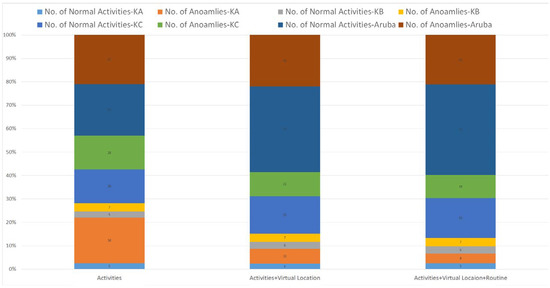
Figure 11. Results of anomaly detection.

5. Conclusions

This study introduces the concept of the virtual location to address the problem of discovering periodic behavior routines for smart home residents without prior knowledge of where sensors are geographically deployed. This concept extracts spatial features from the implicit correlations among sensors, creates an abstract spatial representation of the physical environment, and assigns sensors with strong correlations to the same virtual location. An unsupervised approach to discovering periodic behavioral routines and solutions for potential deviations that considers the length of the discovered activities and transition probabilities among activities create an opportunity for more potential applications in smart homes. Furthermore, with these advantages, the proposed method provides great flexibility for the application of smart home monitoring techniques to households and could be helpful for home automation for the elderly who live independently and require timely interventions. The experimental results show that with the help of virtual location, the proposed method can achieve up to 93% accuracy in activity discovery. The computational time required to complete the task is at least two times less than without the help of the virtual location. In addition, we also demonstrated the applicability of the routine discovery process in behavioral anomaly detection. The results show that virtual location and routine discovery can tolerate variance in behavior routines and provide more accurate inference when determining whether the current activity has deviated from periodic behavior routines.

References

- Bandyopadhyay, D.; Sen, J. Internet of Things: Applications and challenges in technology and standardization. Wirel. Pers. Commun. 2011, 58, 49–69. [Google Scholar] [CrossRef] [Green Version]
- Akhund, T.M.N.U.; Roy, G.; Adhikary, A.; Alam, M.A.; Newaz, N.T.; Rana Rashel, M.; Abu Yousuf, M. Snappy wheelchair: An IoT-based flex controlled robotic wheel chair for disabled people. In Proceedings of the Fifth International Conference on Information and Communication Technology for Competitive Strategies (ICTCS), Jaipur, India, 11–12 December 2020; pp. 803–812. [Google Scholar]
- Kinsella, K.; Beard, J.; Suzman, R. Can populations age better, not just live longer? Generations 2013, 37, 19–26. [Google Scholar]
- Huang, T.; Huang, C. Attitudes of the elderly living independently towards the use of robots to assist with activities of daily living. Work 2021, 69, 1–11. [Google Scholar] [CrossRef]
- Barigozzi, F.; Turati, G. Human health care and selection effects. Understanding labor supply in the market for nursing. Health Econ. 2012, 21, 477–483. [Google Scholar] [CrossRef] [PubMed]
- Yacchirema, D.; de Puga, J.S.; Palau, C.; Esteve, M. Fall detection system for elderly people using IoT and ensemble machine learning algorithm. Pers. Ubiquitous Comput. 2019, 23, 801–817. [Google Scholar] [CrossRef]
- Javaid, M.; Haleem, A.; Rab, S.; Pratap Singh, R.; Suman, R. Sensors for daily life: A review. Sens. Int. 2021, 2, 100121. [Google Scholar] [CrossRef]
- Akbari, S.; Haghighat, F. Occupancy and occupant activity drivers of energy consumption in residential buildings. Energy Build. 2021, 250, 111303. [Google Scholar] [CrossRef]
- Ariano, R.; Manca, M.; Paternò, F.; Santoro, C. Smartphone-based augmented reality for end-user creation of home automations. Behav. Inf. Technol. 2021, 42, 1–17. [Google Scholar] [CrossRef]
- Rodrigues, M.J.; Postolache, O.; Cercas, F. Physiological and behavior monitoring systems for smart healthcare environments: A review. Sensors 2020, 20, 2186. [Google Scholar] [CrossRef] [Green Version]
- Bakar, U.A.B.U.A.; Ghayvat, H.; Hasanm, S.F.; Mukhopadhyay, S.C. Activity and anomaly detection in smart home: A survey. Next Gener. Sens. Syst. 2016, 16, 191–220. [Google Scholar]
- Demiris, G.; Hensel, B.K. Technologies for an aging society: A systematic review of smart home applications. Yearb. Med. Inform. 2008, 17, 33–40. [Google Scholar]
- Akl, A.; Taati, B.; Mihailidis, A. Autonomous unobtrusive detection of mild cognitive impairment in older adults. IEEE Trans. Biomed. Eng. 2015, 62, 1383–1394. [Google Scholar] [CrossRef] [Green Version]
- Elhamshary, M.; Youssef, M.; Uchiyama, A.; Yamaguchi, H.; Higashino, T. TransitLabel: A crowd-sensing system for automatic labeling of transit stations semantics. In Proceedings of the 14th ACM International Conference on Mobile Systems, Applications, and Services (MobiSys), Singapore, 26–30 June 2016; pp. 193–206. [Google Scholar]
- Brush, A.J.; Lee, B.; Mahajan, R.; Agarwal, S.; Saroiu, S.; Dixon, C. Home automation in the wild: Challenges and opportunities. In Proceedings of the International Conference on Human Factors in Computing Systems(CHI), Vancouver, BC, Canada, 7–12 May 2011; pp. 2115–2124. [Google Scholar]
- Friedrich, B.; Sawabe, T.; Hein, A. Unsupervised statistical concept drift detection for behaviour abnormality detection. Appl. Intell. 2022, 53, 2527–2537. [Google Scholar] [CrossRef]
- Esposito, L.; Leotta, F.; Mecella, M.; Veneruso, S. Unsupervised segmentation of smart home logs for human habit discovery. In Proceedings of the 2022 18th International Conference on Intelligent Environments (IE), Biarritz, France, 20–23 June 2022; pp. 1–8. [Google Scholar]
- Perera, C.; Zaslavsky, A.; Christen, P.; Georgakopoulos, D. Context aware computing for the Internet of Things: A survey. IEEE Commun. Surv. Tutor. 2014, 16, 414–454. [Google Scholar] [CrossRef] [Green Version]
- Augusto, J.C.; Nugent, C.D. Smart homes can be smarter. Lect. Notes Comput. Sci. 2006, 4008, 1–15. [Google Scholar]
- Yao, L.; Sheng, Q.Z.; Benatallah, B.; Dustdar, S.; Wang, X.; Shemshadi, A.; Kanhere, S.S. WITS: An IoT-endowed computational framework for activity recognition in personalized smart home. Computing 2018, 100, 369–385. [Google Scholar] [CrossRef]
- Augusto, J.C.; Liu, J.; McCullagh, P.; Wang, H. Management of uncertainty and spatio-temporal aspects for monitoring and diagnosis in a smart home. Int. J. Comput. Intell. 2008, 1, 361–378. [Google Scholar]
- Lymberopoulos, D.; Bamis, A.; Savvides, A. Extracting spatiotemporal human activity patterns in assisted living using a home sensor network. Univers. Access Inf. Soc. 2011, 10, 125–138. [Google Scholar] [CrossRef] [Green Version]
- Azizyan, M.; Constandache, I.; Choudhury, R.R. SurroundSense: Mobile phone localization via ambience fingerprinting. In Proceedings of the 15th Annual International Conference on Mobile Computing and Networking (MobiCom), Beijing, China, 20–25 September 2009; pp. 261–272. [Google Scholar]
- Fan, M.; Adams, A.T.; Truong, K.N. Public restroom detection on mobile phone via active probing. In Proceedings of the 2014 ACM International Symposium on Wearable Computers (ISWC), Seattle, WA, USA, 13–17 September 2014; pp. 27–34.
- Chen, C.; Ren, Y.; Liu, H.; Chen, Y.; Li, H. Acoustic-sensing-based location semantics identification using smartphones. IEEE Internet Things J. 2022, 9, 20640–20650. [Google Scholar] [CrossRef]
- Gozick, B.; Subbu, K.P.; Dantu, R.; Maeshiro, T. Magnetic maps for indoor navigation. IEEE Trans. Instrum. Meas. 2011, 60, 3883–3891. [Google Scholar] [CrossRef]
- Borelli, E.; Paolini, G.; Antoniazzi, F.; Barbiroli, M.; Benassi, F.; Chesani, F.; Chiari, L.; Fantini, M.; Fuschini, F.; Galassi, A.; et al. HABITAT: An IoT solution for independent elderly. Sensors 2019, 19, 1258. [Google Scholar] [CrossRef] [PubMed] [Green Version]
- Ji, Y.; Zhao, X.; Wei, Y.; Wang, C. Generating indoor Wi-Fi fingerprint map based on crowdsourcing. Wirel. Netw. 2022, 28, 1053–1065. [Google Scholar] [CrossRef]
- Tapia, E.M.; Intille, S.S.; Larson, K. Activity recognition in the home using simple and ubiquitous sensors. Lect. Notes Comput. Sci. 2004, 3001, 158–175. [Google Scholar]
- Cook, D.J.; Crandall, A.S.; Thomas, B.L.; Krishnan, N.C. CASAS: A smart home in a box. Computer 2013, 46, 62–69. [Google Scholar] [CrossRef] [PubMed] [Green Version]
- Heierman, E.O.; Youngblood, M.; Cook, D.J. Mining temporal sequences to discover interesting patterns. In Proceedings of the KDD Workshop on Mining Temporal and Sequential Data (KDD), Seattle, WA, USA, 22–25 August 2004. [Google Scholar]
- Rissanen, J. Stochastic Complexity in Statistical Inquiry; World Scientific Publishing: Singapore, 1989. [Google Scholar]
- Cook, D.J.; Youngblood, M.; Heierman, E.O.; Gopalratnam, K.; Rao, S.; Litvin, A.; Khawaja, F. MavHome: An agent-based smart home. In Proceedings of the First IEEE International Conference on Pervasive Computing and Communications (PerCom), Fort Worth, TX, USA, 26 March 2003; pp. 521–524. [Google Scholar]
- Viard, K.; Fanti, M.P.; Faraut, G.; Lesage, J.-J. Human activity discovery and recognition using probabilistic finite-state automata. IEEE Trans. Autom. Sci. Eng. 2020, 17, 2085–2096. [Google Scholar] [CrossRef]
- Reyes-Campos, J.; Alor-Hernández, G.; Machorro-Cano, I.; Olmedo-Aguirre, J.O.; Sánchez-Cervantes, J.L.; Rodríguez-Mazahua, L. Discovery of resident behavior patterns using machine learning techniques and IoT paradigm. Mathematics 2021, 9, 219. [Google Scholar] [CrossRef]
- Papadopoulos, S.; Kompatsiaris, Y.; Vakali, A.; Spyridonos, P. Community detection in social media. Data Min. Knowl. Discov. 2012, 24, 515–554. [Google Scholar] [CrossRef]
- Wanga, T.; Yin, L.; Wang, X. A community detection method based on local similarity and degree clustering information. Physica A 2018, 490, 1344–1354. [Google Scholar] [CrossRef]
- Shin, H.; Park, J.; Kang, D. A graph-cut-based approach to community detection in networks. Appl. Sci. 2022, 12, 6218. [Google Scholar] [CrossRef]
- Blondel, V.D.; Guillaume, J.L.; Lambiotte, R.; Lefebvre, E. Fast unfolding of communities in large networks. J. Stat. Mech.: Theory Exp. 2008, 2008, 10008. [Google Scholar] [CrossRef] [Green Version]
- Aynaud, T.; Blondel, V.D.; Guillaume, J.L.; Lambiotte, R. Multilevel local optimization of modularity. In Graph Partitioning; John Wiley & Sons: New York, NY, USA, 2013; pp. 315–345. [Google Scholar]
- Newaz, N.T.; Haque, M.R.; Akhund, T.M.N.U.; Khatun, T.; Biswas, M. IoT security perspectives and probable solution. In Proceedings of the 2021 Fifth World Conference on Smart Trends in Systems Security and Sustainability (WorldS4), London, UK, 29–30 July 2021; pp. 81–86. [Google Scholar]
- Lo, C.-C.; Hsu, K.-H.; Horng, M.-F.; Kuo, Y.-H. Spatial Information Extraction using Hidden Correlations. In Proceedings of the 2018 IEEE 29th Annual International Symposium on Personal, Indoor and Mobile Radio Communications (PIMRC), Bologna, Italy, 9–12 September 2018; pp. 1–6. [Google Scholar]
- Qin, S.M.; Verkasalo, H.; Mohtaschemi, M.; Hartonen, T.; Alava, M. Patterns, entropy, and predictability of human mobility and life. PLoS ONE 2012, 7, e51353. [Google Scholar] [CrossRef] [Green Version]
- Kolmogorov, A.N.; Uspenskii, V.A. Algorithms and randomness. Theory Probab. Appl. 1988, 32, 389–412. [Google Scholar] [CrossRef] [Green Version]
- Chifu, V.R.; Pop, C.B.; Demjen, D.; Socaci, R.; Todea, D.; Antal, M.; Cioara, T.; Anghel, I.; Antal, C. Identifying and Monitoring the Daily Routine of Seniors Living at Home. Sensors 2022, 22, 992. [Google Scholar] [CrossRef]
- Borgelt, C. Simple algorithms for frequent item set mining. In Advances in Machine Learning II; Springer: Berlin/Heidelberg, Germany, 2010; pp. 351–369. [Google Scholar]
- van Kasteren, T.L.M.; Englebienne, G.; Kröse, B.J.A. Human activity recognition from wireless sensor network data: Benchmark and software. In Activity Recognition in Pervasive Intelligent Environments of the Atlantis Ambient and Pervasive Intelligence Series; Atlantis Press: Paris, France, 2011; pp. 165–186. [Google Scholar]
- Cook, D.J. Learning setting-generalized activity models for smart spaces. IEEE Intell. Syst. 2012, 27, 32–38. [Google Scholar] [CrossRef]
- Rosenberg, A.; Hirschberg, J. V-measure: A conditional entropy-based external cluster evaluation measure. In Proceedings of the 2007 Joint Conference on Empirical Methods in Natural Language Processing and Computational Natural Language Learning (EMNLP-CoNLL), Prague, Czech Republic, 28–30 June 2007; pp. 410–420. [Google Scholar]
Disclaimer/Publisher’s Note: The statements, opinions and data contained in all publications are solely those of the individual author(s) and contributor(s) and not of MDPI and/or the editor(s). MDPI and/or the editor(s) disclaim responsibility for any injury to people or property resulting from any ideas, methods, instructions or products referred to in the content. |
© 2023 by the authors. Licensee MDPI, Basel, Switzerland. This article is an open access article distributed under the terms and conditions of the Creative Commons Attribution (CC BY) license (https://creativecommons.org/licenses/by/4.0/).