Stabilization of Stochastic Dynamical Systems of a Random Structure with Markov Switches and Poisson Perturbations

Abstract

An optimal control for a dynamical system optimizes a certain objective function. Here, we consider the construction of an optimal control for a stochastic dynamical system with a random structure, Poisson perturbations and random jumps, which makes the system stable in probability. Sufficient conditions of the stability in probability are obtained, using the second Lyapunov method, in which the construction of the corresponding functions plays an important role. Here, we provide a solution to the problem of optimal stabilization in a general case. For a linear system with a quadratic quality function, we give a method of synthesis of optimal control based on the solution of Riccati equations. Finally, in an autonomous case, a system of differential equations was constructed to obtain unknown matrices that are used for the construction of an optimal control. The method using a small parameter is justified for the algorithmic search of an optimal control. This approach brings a novel solution to the problem of optimal stabilization for a stochastic dynamical system with a random structure, Markov switches and Poisson perturbations.

1. Introduction

The main problem considered in this paper is the synthesis of an optimal control for a controlled dynamical system, described by a stochastic differential equation (SDE) with Poisson perturbations and external random jumps [1,2]. The importance of this problem is linked to the fact that the dynamics of many real processes cannot be described by continuous models such as ordinary differential equations or Ito’s stochastic differential equations [3]. More complex systems include the presence of jumps, and these jumps can occur at random ${\tau }_k,k\ge 1$, or deterministic time moments, $t_m,m\ge 1$. In the first case, the jump-like change can be described by point processes [4,5], or in a more specific case by generalized Poisson processes, the dynamics of which are characterized only by the intensity of the jumps. The jumps of the system at deterministic moments of time, $t_m$, can be described by the relation:

$$\mathsf{\Delta }x\left(t_m\right)=x\left(t_m\right)-x(t_m-)=g(\dots ),$$

(1)

where $x\left(t\right),t\ge 0$, is a random process describing the dynamics of the system, the function g is a finite-valued function that reflects the magnitude of a jump which depends on time t and process x in the time $t_m-$. According to the works of Katz I. Ya. [1], Yasinsky V.K., Yurchenko I.V. and Lukashiv T.O. [6], the description of jumps at deterministic time moments, $t_m$, are quite accurately described using the Equation (1). It allows a relatively simple transfer of the basic properties of stochastic systems of differential equations without jumps ($g\equiv 0$) to systems with jumps. Such properties, as will be noted below, include the Markovian property, $x\left(t\right),t\ge 0$, concerning natural filtering, and the martingale properties, ${\parallel x\left(t\right)\parallel }^2,t\ge 0$ [7,8]. It should be noted that the description of real dynamical systems is not limited to the Wiener process and point processes (Poisson process). A more general approach is based on the use of semimartingales [9]. The disadvantage of this approach is that it is impossible to link it with the methods used for systems described by ordinary differential equations or stochastic Ito’s differential equations. The second approach to describe jump processes, $x\left(t\right)$, is based on the use of semi-Markov processes, considered in the works of Korolyuk V.S. [10] and Malyk I.V. [2,11]. In particular, the works of Malyk I.V. are devoted to the convergence of semi-Markov evolutions in the averaging scheme and diffusion approximation. The results derived in these works together with the results of the works on large deviations (e.g., [12]) can also be used to investigate the considered problems.

Since we consider generalized classical differential equations, the approaches used will also be classical. The basic research method is based on the Lyapunov methods described in the papers by Katz I. Ya. [1] and Lukashiv T.O. and Malyk I.V. [13]. It should be noted that the application of this method makes it possible to find the optimal control for linear systems with a quadratic quality functional, which also corresponds to classical dynamical systems [14].

It should be noted that a large number of works are devoted to the issues of stability of systems with jumping Markov processes. For example, the works [15,16] consider sufficient conditions for the stability of Ito stochastic differential equations with Markov switching and the presence of variable delay. In the work [15], this theory has gained logical use for modeling neural networks with a decentralized event-triggered mechanism and finding sufficient conditions for stabilizing the process that describe dynamic of the neural network. Note that the authors of this work also considered systems of stochastic differential equations in which the deterministic term near $dt$ is quasi-linear; that is, the linear component plays the main role in this research. This assumption of quasi-linearity allows, with additional conditions on the value of the nonlinear part, the discovery of sufficient stability conditions of the $x\left(t\right),t\ge 0,$ by constructing suboptimal control $u\left(t\right),t\ge 0$. Similar results were obtained also in the work [16], where authors described an algorithm of stabilization by construction of the non-fragile event-triggered controller for Ito stochastic differential equations with varying delay. The authors chose a specific class of admissible controls, which makes it possible to solve the optimization problem for finding a suboptimal control.

The structure of the paper is as follows. In Section 2, we consider the mathematical model of a dynamical system with jumps. It is described by a system of stochastic differential equations with Poisson’s integral and external jumps. Sufficient conditions for the existence and uniqueness of the solution of this system are given there. In Section 3, we investigate the stability in probability of the solution $x\left(t\right),t\ge 0$. In this section, we consider the notion of the Lyapunov function and prove the sufficient conditions for stability in probability (Theorem 1). The algorithm for computing the quality functional, $J_u(y,h,x_0)$, from the known control, $u\left(t\right)$, is given in Section 4. Moreover, we further present sufficient conditions for the existence of an optimal control (Theorem 2), which are based on the existence of a Lyapunov function for the given system. Section 5 considers constructing an optimal control for linear non-autonomous systems via the coefficients of the system. The optimal control is found by solving auxiliary Ricatti equations (Theorem 3). For the analysis of linear autonomous systems, we consider the construction of a quadratic functional. Finally, we formulate sufficient conditions of existence of an optimal control (Theorem 4), and present the explicit form of such a control in the case of a quadratic quality functional.

2. Task Definition

On the probability basis $(\mathsf{\Omega },\mathfrak{F},F,\mathbf{P})$ [7], consider a stochastic dynamical system of a random structure given by Ito’s stochastic differential Equation (SDE) with Poisson perturbations:

$$dx\left(t\right)=a(t-,\xi (t-),x(t-),u(t-\left)\right)dt+$$

$$+b(t-,\xi (t-),x(t-),u(t-\left)\right)dw\left(t\right)+$$

$$+\underset{{\mathbb{R}}^m}{\int }\left(c(t-,\xi (t-),x(t-),u(t-),z)\right)\tilde{\nu }(dz,dt),t\in {\mathbb{R}}_{+}\setminus K,$$

(2)

with Markov switches

$$\mathsf{\Delta }x\left(t\right){|}_{t=t_k}=g(t_k-,\xi (t_k-),{\eta }_k,x(t_k-)),t_k\in K=\{t_n\Uparrow \}$$

(3)

for $\underset{n\to +\infty }{lim}{t}_n=+\infty$ and initial conditions

$$x\left(0\right)=x_0\in {\mathbb{R}}^m,\xi \left(0\right)=y\in \mathbf{Y},{\eta }_0=h\in \mathbf{H}.$$

(4)

Here, $\xi \left(t\right),t\ge 0,$ is a homogeneous continuous Markov process with a finite number of states $\mathbf{Y}:=\{y_1,\dots ,y_N\}$ and a generator Q; $\{{\eta }_k,k\ge 0\}$ is a Markov chain with values in the space $\mathbf{H}$ and the transition probability matrix ${\mathbb{P}}_H$; $x:[0,+\infty )\times \mathsf{\Omega }\to {\mathbb{R}}^m$; $w\left(t\right)$ is an m-dimensional standard Wiener process; $\tilde{\nu }(dz,dt)=\nu (dz,dt)-\mathbb{E}\nu (dz,dt)$ is a centered Poisson measure; and the processes $w,\nu ,\xi$ and $\eta$ are independent [3,7]. We denote by

$${\mathfrak{F}}_{t_k}=\sigma (\xi \left(s\right),w\left(s\right),\nu (s,*),{\eta }_e,s\le t_k,t_e\le t_k)$$

a minimal $\sigma$-algebra, with respect to which $\xi \left(t\right)$ is measurable for all $t\in [0,t_k]$ and ${\eta }_n$ for $n\le k$.

The process $x\left(t\right),t\ge 0$ is $c\stackrel{`}{a}dl\stackrel{`}{a}g$ and the control $u\left(t\right):=u(t,x\left(t\right)):[0,T]\times {\mathbb{R}}^m\to {\mathbb{R}}^m$ is an m-measure function from the class of admissible controls U [14].

The following mappings are measurable by a set of variables $a:{\mathbb{R}}_{+}\times \mathbf{Y}\times {\mathbb{R}}^m\times {\mathbb{R}}^m\to {\mathbb{R}}^m$, $b:{\mathbb{R}}_{+}\times \mathbf{Y}\times {\mathbb{R}}^m\times {\mathbb{R}}^m\to {\mathbb{R}}^m\times {\mathbb{R}}^m$, $c:{\mathbb{R}}_{+}\times \mathbf{Y}\times {\mathbb{R}}^m\times {\mathbb{R}}^m\times {\mathbb{R}}^m\to {\mathbb{R}}^m$ and function $g:{\mathbb{R}}_{+}\times \mathbf{Y}\times \mathbf{H}\times {\mathbb{R}}^m\to {\mathbb{R}}^m$ satisfies the Lipschitz condition

$$|a(t,y,x_1,u)-a(t,y,x_2,u)|+|b(t,y,x_1,u)-b(t,y,x_2,u)|+$$

$$+\underset{{\mathbb{R}}^m}{\int }|c(t,y,x_1,u,z)-c(t,y,x_2,u,z)|\mathsf{\Pi }\left(dz\right)+$$

$$+|g(t,y,h,x_1)-g(t,y,h,x_2)|\le L|x_1-x_2|,$$

(5)

where $\mathsf{\Pi }\left(dz\right)$ is defined by $\mathbb{E}\nu (dz,dt)=\mathsf{\Pi }\left(dz\right)dt$, $L>0$, $x_1,x_2\in {\mathbb{R}}^m$ for $\forall t\ge 0,y\in \mathbf{Y},h\in \mathbf{H}$, and the condition

$$\left|a(t,y,0,u)\right|+\left|b(t,y,0,u)\right|+\underset{{\mathbb{R}}^m}{\int }\left|c(t,y,0,u,z)\right|\mathsf{\Pi }\left(dz\right)+$$

$$+\left|g\right(t,y,h,0\left)\right|\le C<\infty ,$$

(6)

The conditions defined above, with respect to the mappings $a,b,c$ and g, guarantee the existence of a strong solution to Equations (2)–(4) with the exact stochastic equivalence [13].

Let us denote

$${\mathbf{P}}_k((y,h,x),\mathsf{\Gamma }\times G\times \mathbf{C}):=$$

$$:=P(\xi \left(t_{k+1}\right),{\eta }_{k+1},x\left(t_{k+1}\right)\in \mathsf{\Gamma }\times G\times \mathbf{C}|(\xi \left(t_k\right),{\eta }_k,x\left(t_k\right))=(y,h,x))$$

the transition probability of a Markov chain $(\xi \left(t_k\right),{\eta }_k,x\left(t_k\right))$, determining the solution to the Equations (2)–(4) $x\left(t\right)$, at the k-th step.

3. Stability in Probability

Here we used the definitions from classical works in this area [14,17].

Definition 1. 

The discrete Lyapunov operator $\left(l{v}_k\right)(y,h,x)$ on a sequence of measurable scalar functions $v_k(y,h,x):\mathbf{Y}\times \mathbf{H}\times {\mathbb{R}}^m\to {\mathbb{R}}^1,k\in \mathbb{N}\cup \left\{0\right\}$ for SDE (2) with Markov switches (3) is defined by the equation:

$$\left(l{v}_k\right)(y,h,x):=\underset{\mathbf{Y}\times \mathbf{H}\times {\mathbb{R}}^m}{\int }{\mathbf{P}}_k((y,h,x),du\times dz\times dl)v_{k+1}(u,z,l)-v_k(y,h,x),k\ge 0.$$

(7)

When applying the second Lyapunov method to the SDE (2) with Markov switches (3), special sequences of the above mentioned functions $v_k(y,h,x),k\in \mathbb{N}$ are required.

Definition 2. 

The Lyapunov function for the system of the random structure (2)–(4) is a sequence of non-negative functions $\left\{v_k(y,h,x),k\ge 0\right\},$ for which

• for all $k\ge 0,y\in \mathbf{Y},h\in \mathbf{H},x\in {\mathbb{R}}^m$ the discrete Lyapunov operator is defined $\left(l{v}_k\right)(y,h,x)$ (7);
• for $r\to \infty$

  $$\overline{v}\left(r\right)\equiv \underset{\begin{array}{c}k\in \mathbb{N},y\in \mathbf{Y},\hfill \\ h\in \mathbf{H},\left|x\right|\ge r\hfill \end{array}}{inf{v}_k}(y,h,x)\to +\infty$$
• for $r\to 0$

  $$\underline{v}\left(r\right)\equiv \underset{\begin{array}{c}k\in \mathbb{N},y\in \mathbf{Y},\hfill \\ h\in \mathbf{H},\left|x\right|\le r\hfill \end{array}}{sup{v}_k}(y,h,x)\to 0,$$

Moreover, $\overline{v}\left(r\right)$ and $\underline{v}\left(r\right)$ are continuous and strictly monotonous.

Definition 3. 

Let us call a system of random structure (2)–(4) stable in probability on the whole, and if for $\forall {\epsilon }_1>0,{\epsilon }_2>0$ one can specify, as $\delta >0$, that from the inequality $\left|x\right|<\delta$ follows the inequality

$$\mathbf{P}\left\{\underset{t\ge 0}{sup}\left|x\left(t\right)\right|>{\epsilon }_1\right\}<{\epsilon }_2$$

(8)

for all $x_0\in {\mathbb{R}}^m$, $y\in \mathbf{Y},h\in \mathbf{H}$.

To solve the Equations (2)–(4) in the intervals $[t_k,t_{k+1})$, the following estimate takes place.

Lemma 1. 

Let the coefficients of Equation (2), $a,b,c$ and function g, satisfy the Lipschitz condition (5) and the uniform boundedness condition (6).

Then, for all $k\ge 0$, the inequality for the strong solution of the Cauchy problem (2)–(4) holds

$$\mathbf{E}\left\{\underset{t_k\le t<t_{k+1}}{sup}{\left|x\left(t\right)\right|}^2\right\}\le 7\left[\mathbb{E}{\left|x\left(t_k\right)\right|}^2+3C^2(t_{k+1}-t_k)\right]\times$$

$$\times exp\left\{7L^2((t_{k+1}-t_k)+8)\right\},t\in (t_k,t_{k+1}).$$

(9)

Proof of Lemma 1 

Using the integral form of the strong solution of Equation (2) [8], for all $t\in [t_k,t_{k+1}),t_k\ge 0,$ the following inequality is true:

$$\left|x\left(t\right)\right|\le \left|x\left(t_k\right)\right|+{\int }_{t_k}^t\left|a(\tau ,\xi (\tau ),x(\tau ),u(\tau \left)\right)-a(\tau ,\xi (\tau ),0,u(\tau \left)\right)\right|d\tau +$$

$$+\underset{t_k}{\overset{t}{\int }}\left|a(\tau ,\xi (\tau ),0,u(\tau \left)\right)\right|d\tau +$$

$$+\underset{t_k}{\overset{t}{\int }}\left|b(\tau ,\xi (\tau ),x(\tau ),u(\tau \left)\right)-b(\tau ,\xi (\tau ),0,u(\tau \left)\right)\right|dw\left(\tau \right)+$$

$$+{\int }_{t_k}^t\left|b(\tau ,\xi (\tau ),0,u(\tau \left)\right)\right|dw\left(\tau \right)+$$

$$+\underset{t_k}{\overset{t}{\int }}\underset{{\mathbb{R}}^m}{\int }\left|c(\tau ,\xi (\tau ),x(\tau ),u(\tau ),z)-c(\tau ,\xi (\tau ),0,u(\tau ),z)\right|\tilde{\nu }(dz,d\tau )+$$

$$+\underset{t_k}{\overset{t}{\int }}\underset{{\mathbb{R}}^m}{\int }\left|c(\tau ,\xi (\tau ),0,u(\tau ),z)\right|\tilde{\nu }(dz,d\tau )$$

Given (5) and (6) and the inequality ${\left({\sum }_{i=1}^n{x}_i\right)}^2\le n{\sum }_{i=1}^n{x}_i^2$ we get:

$$\underset{t_k\le t<t_{k+1}}{sup}{\left|x\left(t\right)\right|}^2\le 7\underset{t_k\le t<t_{k+1}}{sup}\left[{\left|x\left(t_k\right)\right|}^2+\right.$$

$$+{\left|{\int }_{t_k}^t\left|a(\tau ,\xi (\tau ),x(\tau ),u(\tau \left)\right)-a(\tau ,\xi (\tau ),0,u(\tau \left)\right)\right|d\tau \right|}^2+$$

$$+{\left|\underset{t_k}{\overset{t}{\int }}\left|a(\tau ,\xi (\tau ),0,u(\tau \left)\right)\right|d\tau \right|}^2+$$

$$+{\left|\underset{t_k}{\overset{t}{\int }}\left|b(\tau ,\xi (\tau ),x(\tau ),u(\tau \left)\right)-b(\tau ,\xi (\tau ),0,u(\tau \left)\right)\right|dw\left(\tau \right)\right|}^2+$$

$$+{\left|{\int }_{t_k}^t\left|b(\tau ,\xi (\tau ),0,u(\tau \left)\right)\right|dw\left(\tau \right)\right|}^2+$$

$$+{\left|\underset{t_k}{\overset{t}{\int }}\underset{{\mathbb{R}}^m}{\int }\left|c(\tau ,\xi (\tau ),x(\tau ),u(\tau ),z)-c(\tau ,\xi (\tau ),0,u(\tau ),z)\right|\tilde{\nu }(dz,d\tau )\right|}^2+$$

$$+\left.{\left|\underset{t_k}{\overset{t}{\int }}\underset{{\mathbb{R}}^m}{\int }\left|c(\tau ,\xi (\tau ),0,u(\tau ),z)\right|\tilde{\nu }(dz,d\tau )\right|}^2\right]\le$$

$$\le 7\left[\underset{t_k\le t<t_{k+1}}{sup}{\left|x\left(t\right)\right|}^2+\underset{t_k\le t<t_{k+1}}{sup}{L}^2{\left|\underset{t_k}{\overset{t}{\int }}\left|x\left(\tau \right)\right|d\tau \right|}^2+\right.$$

$$+C^2(t_{k+1}-t_k)+\underset{t_k\le t<t_{k+1}}{sup}{L}^2{\left|\underset{t_k}{\overset{t}{\int }}\left|x\left(\tau \right)\right|dw\left(\tau \right)\right|}^2+C^2(t_{k+1}-t_k)+$$

$$+\underset{t_k\le t<t_{k+1}}{sup}{\left|\underset{t_k}{\overset{t}{\int }}\underset{{\mathbb{R}}^m}{\int }\left|c(\tau ,\xi (\tau ),x(\tau ),u(\tau ),z)-c(\tau ,\xi (\tau ),0,u(\tau ),z)\right|\tilde{\nu }(dz,d\tau )\right|}^2+$$

$$+\left.\underset{t_k\le t<t_{k+1}}{sup}{\left|\underset{t_k}{\overset{t}{\int }}\underset{{\mathbb{R}}^m}{\int }\left|c(\tau ,\xi (\tau ),0,u(\tau ),z)\right|\tilde{\nu }(dz,d\tau )\right|}^2\right].$$

Consider the designation:

$$y\left(t\right)=\mathbb{E}\left\{\underset{t_k\le s<t}{sup}{\left|x\left(s\right)\right|}^2/{\mathfrak{F}}_{t_k}\right\}.$$

Then, according to the last inequality, $y\left(t\right)$ satisfies the ratio:

$$y\left(t\right)\le 7\left[\mathbb{E}\left\{{\left|x\left(t\right)\right|}^2/{\mathfrak{F}}_{t_k}\right\}+3C^2(t_{k+1}-t_k)+L^2((t_{k+1}-t_k)+8)·\underset{t_k}{\overset{t}{\int }}y\left(\tau \right)d\tau \right].$$

Using the Gronwall inequality, we obtain an estimate of:

$$\mathbb{E}\left\{\underset{t_k\le t<t_{k+1}}{sup}{\left|x\left(t\right)\right|}^2/{\mathfrak{F}}_{t_k}\right\}\le$$

$$\le 7\left[\mathbb{E}{\left|x\left(t_k\right)\right|}^2+3C^2(t_{k+1}-t_k)\right]e^{7L^2\left((t_{k+1}-t_k)+8\right)},$$

as required as proof.

□

Remark 1. 

We will consider the stability of the trivial solution $x\equiv 0$ of the system (2)–(4); that is, the fulfillment of (6) when $C=0$ [17,18,19].

Theorem 1. 

Let:

(1) 

Interval lengths $[t_k,t_{k+1})$ do not exceed $\mathsf{\Delta }>0$, i.e., $\left|t_{k+1}-t_k\right|\le \mathsf{\Delta },k\ge 0;$

(2) 

The Lipschitz condition is satisfied (5);

(3) 

There exists Lyapunov functions $v_k(y,h,x),k\ge 0$ such that the following inequality holds true

$$\left(l{v}_k\right)(y,h,x)\le 0,k\ge 0.$$

(10)

Then, the system of random structure (2)–(4) is stable in probability on the whole.

Remark 2. 

It should be noted that if condition 1 is not satisfied, the number of jumps (3) is finite and the system (2)–(4) turns into a system without jumps after $max{t}_k$. In this case, we can use the results presented in [1].

Proof of Theorem 1 

The conditional expectation of the Lyapunov function is:

$$\mathbf{E}\left\{v_{k+1}(\xi \left(t_{k+1}\right),{\eta }_{k+1},x\left(t_{k+1}\right))/\phantom{v_{k+1}(\xi \left(t_{k+1}\right),{\eta }_{k+1},x\left(t_{k+1}\right)){\mathfrak{F}}_{t_k}}{\mathfrak{F}}_{t_k}\right\}={\int }_{\mathbf{Y}\times \mathbf{H}\times {\mathbb{R}}^m}{\mathbf{P}}_k\left((\xi \left(t_k\right),{\eta }_k,x\left(t_k\right))(du\times dz\times dl)v_{k+1}(u,z,l)\right).$$

(11)

Then, by the definition of the discrete Lyapunov operator $\left(l{v}_k\right)(y,h,x)$ (see (7)) and from Equation (11), taking into account (10), we obtain the following inequality:

$$\mathbf{E}\left\{v_{k+1}(\xi \left(t_{k+1}\right),{\eta }_{k+1},x\left(t_{k+1}\right))/\phantom{v_{k+1}(\xi \left(t_{k+1}\right),{\eta }_{k+1},x\left(t_{k+1}\right)){\mathfrak{F}}_{t_k}}{\mathfrak{F}}_{t_k}\right\}=v_k(\xi \left(t_k\right),{\eta }_k,x\left(t_k\right))+\left(l{v}_k\right)(\xi \left(t_k\right),{\eta }_k,x\left(t_k\right))\le \overline{v}\left(\left|x\left(t_k\right)\right|\right).$$

(12)

From Lemma 1 and the properties of the function $\overline{v}$, it follows that the conditional expectation of the left part of inequality (12) exists.

Using (11) and (12), let us write the discrete Lyapunov operator $\left(l{v}_k\right)(y,h,x)$, defined by the solutions of (2)–(4):

$$\left(l{v}_k\right)(\xi \left(t_k\right),{\eta }_k,x\left(t_k\right))=\mathbf{E}\left\{v_{k+1}(\xi \left(t_{k+1}\right),{\eta }_{k+1},x\left(t_{k+1}\right))/\phantom{v_{k+1}(\xi \left(t_{k+1}\right),{\eta }_{k+1},x\left(t_{k+1}\right)){\mathfrak{F}}_{t_k}}{\mathfrak{F}}_{t_k}\right\}-v_k(\xi \left(t_k\right),{\eta }_k,x\left(t_k\right))\le 0.$$

(13)

Then, when $k\ge 0$, the following inequality is satisfied:

$$\mathbf{E}\left\{v_{k+1}(\xi \left(t_{k+1}\right),{\eta }_{k+1},x\left(t_{k+1}\right))/\phantom{v_{k+1}(\xi \left(t_{k+1}\right),{\eta }_{k+1},x\left(t_{k+1}\right)){\mathfrak{F}}_{t_k}}{\mathfrak{F}}_{t_k}\right\}\le v_k(\xi \left(t_k\right),{\eta }_k,x\left(t_k\right)).$$

This means that the sequence of random variables $v_k(\xi \left(t_k\right),{\eta }_k,x\left(t_k\right))$ is a supermartingale with respect to ${\mathfrak{F}}_{t_k}$ [5].

Thus, the following inequality holds:

$$\mathbf{E}\left\{v_{N+1}(\xi \left(t_{N+1}\right),{\eta }_{N+1},x\left(t_{N+1}\right))\right\}-\mathbf{E}\left\{v_n(\xi \left(t_n\right),{\eta }_n,x\left(t_n\right))\right\}=$$

$$=\sum _{k=n}^N\mathbf{E}\left\{\left(l{v}_k\right)(\xi \left(t_k\right),{\eta }_k,x\left(t_k\right))\right\}\le 0.$$

Since the random variable $\underset{t_k\le t<t_{k+1}}{sup}{\left|x\left(t\right)\right|}^2$ is independent of events of $\sigma$- algebra ${\mathfrak{F}}_{t_k}$ [4], then

$$\mathbf{E}\left\{\underset{t_k\le t<t_{k+1}}{sup}{\left|x\left(t\right)\right|}^2/\phantom{\underset{t_k\le t<t_{k+1}}{sup}{\left|x\left(t\right)\right|}^2{\mathfrak{F}}_{t_k}}{\mathfrak{F}}_{t_k}\right\}=E\left\{\underset{t_k\le t<t_{k+1}}{sup}{\left|x\left(t\right)\right|}^2\right\},$$

i.e., the inequality (9) also holds for the usual expectation

$$\mathbf{E}\left\{\underset{t_k\le t<t_{k+1}}{sup}{\left|x\left(t\right)\right|}^2\right\}\le 7\left[\mathbb{E}{\left|x\right|}^2\right]e^{7L^2\left(\mathsf{\Delta }+8\right)}$$

at $C=0$, assuming that the stability of the trivial solution is investigated.

Then,

$$\mathbf{P}\left\{\underset{t\ge 0}{sup}\left|x\left(t\right)\right|>{\epsilon }_1\right\}=$$

$$=\mathbf{P}\left\{\underset{n\in \mathbb{N}}{sup}\underset{t_{n-1}\le t<t_n}{sup}\left|x\left(t\right)\right|>{\epsilon }_1\right\}\le$$

$$\le \mathbf{P}\left\{\underset{n\in \mathbb{N}}{sup}7e^{7L^2\left(\mathsf{\Delta }+8\right)}\left|x\left(t_{n-1}\right)\right|>{\epsilon }_1\right\}\le$$

$$\le \mathbf{P}\left\{\underset{n\in \mathbb{N}}{sup}\left|x\left(t_{n-1}\right)\right|>\frac{{\epsilon }_1}{7}{e}^{-7L^2\left(\mathsf{\Delta }+8\right)}\right\}\le$$

$$\le \mathbf{P}\left\{\underset{n\in \mathbb{N}}{sup}{v}_{n-1}(\xi \left(t_{n-1}\right),{\eta }_{n-1},x\left(t_{n-1}\right))\ge \overline{v}\left(\frac{{\epsilon }_1}{7}{e}^{-7L^2\left(\mathsf{\Delta }+8\right)}\right)\right\}$$

(14)

If $sup\left|x\left(t_k\right)\right|\ge r$, then based on the definition of the Lyapunov function, the inequality is fulfilled

$$\underset{k\ge 0}{sup}{v}_k(\xi \left(t_k\right),{\eta }_k,x\left(t_k\right))\ge \underset{k\ge 0,y\in \mathbf{Y},h\in \mathbf{H},\left|x\right|\ge r}{inf}{v}_k(y,h,x)=\overline{v}\left(r\right).$$

(15)

Using the inequality for non-negative supermartingales [5,7], we obtain an estimate of the right-hand side of (14):

$$\mathbf{P}\left\{\underset{n\in \mathbb{N}}{sup}{v}_{n-1}(\xi \left(t_{n-1}\right),{\eta }_{n-1},x\left(t_{n-1}\right))\ge \overline{v}\left(\frac{{\epsilon }_1}{7}{e}^{-7L^2\left(\mathsf{\Delta }+8\right)}\right)\right\}\le$$

$$\le \frac{1}{\overline{v}\left(\frac{{\epsilon }_1}{7}{e}^{-7L^2\left(\mathsf{\Delta }+8\right)}\right)}{v}_0(y,h,x)\le \frac{\overline{v}\left(\left|x\right|\right)}{\overline{v}\left(\frac{{\epsilon }_1}{7}{e}^{-7L^2\left(\mathsf{\Delta }+8\right)}\right)}.$$

(16)

Given the inequality (14), the inequality (16) guarantees that the inequality (8) of stability in probability holds for the whole system (2)–(4). □

4. Stabilization

The optimal stabilization problem is such that for an SDE (2) with switches (3), one should construct a control $u(t,x(t\left)\right)$ such that the unperturbed motion $x\left(t\right)\equiv 0$ of the system (2)–(4) is stable in probability on the whole.

It is assumed that the control, u, will be determined by the full feedback principle. In addition, the condition of continuity of $u\left(t\right)$ on t is in the range

$$t\ge 0,x\in {\mathbb{R}}^m,y\in \mathbf{Y},h\in \mathbf{H}.$$

(17)

for every fixed $\xi \left(t\right)=y\in \mathbf{Y}$ and ${\eta }_k=h\in \mathbf{H}$.

It is also assumed that the structure of the system at time $t\ge 0$, which is independent of the Markov chain ${\eta }_k$ ($k\ge 0$ corresponds to time $t_k\in K$), is known.

Obviously, there is an infinite set of controls. The only control should be chosen from the requirement of the best quality of the process, which is expressed in the form of the minimization condition of the functional:

$${\mathit{I}}_u(y,h,x_0):=\sum _{k=0}^{\infty }{\int }_{t_k}^{\infty }\mathit{E}\left\{W(t,x\left(t\right),u\left(t\right))/\xi \left(0\right)=y,{\eta }_0=h,x\left(0\right)=x_0\right\}dt,$$

(18)

where $W(t,x,u)\ge 0$ is a non-negative function defined in the region $t\ge 0,x\in {\mathbb{R}}^m$, $u\in {\mathbb{R}}^r$.

The algorithm for calculating the functional (18) for a given control, $u(t,x)$, is as follows:

(A)

Find the trajectory $x\left(t\right)$ with an SDE (2) at $u\equiv u(t,y,h,x)$, for example, by the Euler–Maruyama method [20];

(B)

Substitute $x\left(t\right)$, $\xi \left(t\right)$ and $u\left(t\right)=u(t,x(t\left)\right)$ into the functional (18);

(C)

Calculate the value of the function (18) by statistical modeling (Monte Carlo);

(D)

The problem of choosing the functional $W(t,x,u)$, which determines the estimate ${\mathit{I}}_u$ and the quality of the process $x\left(t\right)$ as a strong solution of the SDE (2), is related to the specific features of the problem and the following three conditions can be identified:

• The minimization conditions of the functional (18) must ensure that the strong solution, $x\left(t\right)$, of the SDE (2) fades fast enough on average with high probability;
• The value of the integral should satisfactorily estimate the computation time spent on generating the control, $u\left(t\right)$;
• The value of the quality functional should satisfactorily estimate the computation time spent on forming the control, $u\left(t\right)$;
• The functional $W(t,x,u)$ must be such that the solution of the stabilization problem can be constructed.

Remark 3. 

For a linear SDE (2), in many cases the quadratic form with respect to the variables x and u is satisfactory

$$W(t,x,u)=x^{T}M\left(t\right)x+u^{T}D\left(t\right)u,$$

(19)

where $M\left(t\right)$ is a symmetric non-negative matrix of size $m\times m$ and $D\left(t\right)$ is a positively determined matrix of the size $r\times r$ for all $t\ge 0$.

Remark 4. 

Note that according to the feedback principle, $M\left(t\right)$ and $D\left(t\right)$ depend indirectly on the values of $\xi \left(t\right)$ and ${\eta }_k$. Therefore, in the examples below, we will calculate the values of $M\left(t\right)$ and $D\left(t\right)$ for fixed $\xi \left(t\right)$ and ${\eta }_k$.

The value ${\mathit{I}}_u$ in the case of the quadratic form of the variables x and u evaluates the quality of the transition process quite well on average. The presence of the term $u^{T}Du$ and the minimum condition simultaneously limit the amount of the control action $u\in {\mathbb{R}}^r$.

Remark 5. 

If the jump condition of the phase trajectory is linear, then the solution of the stabilization problem belongs to the class of linear on the phase vector $x\in {\mathbb{R}}^m$ controls $u(t,x)$. Such problems are called linear-quadratic stabilization problems.

Definition 4. 

The control $u^0\left(t\right)$, which satisfies the condition:

$${\mathit{I}}_{u^0}(y,h,x_0)=min{\mathit{I}}_u(y,h,x_0),$$

where the minimum should be searched for all controls continuous variables t and x at each $\xi \left(0\right)=y\in \mathbf{Y}$ and ${\eta }_0=h\in \mathbf{H}$, let us call it optimal in the sense of optimal stabilization of the strong solution $x\in {\mathbb{R}}^m$ of the system (2)–(4).

Theorem 2. 

Let the system (2)–(4) have a scalar function $v^0(t_k,y,h,x)$ and an r-vector function $u^0(t,y,h,x)\in {\mathbb{R}}^r$ in the region (17) and fulfill the conditions:

1. 

The sequence of the functions $v_k^0(y,h,x)\equiv v^0(t_k,y,h,x)$ is the Lyapunov functional;

2. 

The sequence of r-measured functions-control

$$u_k^0(y,h,x)\equiv u^0(t_k,y,h,x)\in {\mathbb{R}}^{\mathit{r}};$$

(20)

is measurable in all arguments where $0\le t_k<t_{k+1},k\ge 0$;

3. 

The sequence of functions from the criterion (18) by $x\in {\mathbb{R}}^m$ is positive definite, i.e., for $\forall t\in [t_k,t_{k+1}),k\ge 0$,

$$W(t,x,u_k^0(y,h,x))>0;$$

(21)

4. 

The sequence of infinitesimal operators $\left(l{v}_k^0\right){|}_{u_k^0}$, calculated for $u_{{}^k}^0\equiv u^0(y,h,x)$, satisfies the condition for $\forall t\in [t_k,t_{k+1})$

$$\left(l{v}_k^0\right){|}_{u_k^0}=-W(t,x,u_k^0);$$

(22)

5. 

The value of $\left(l{v}_k^0\right)+W(t,x,u)$ reaches a minimum at $u=u^0,k\ge 0$, i.e.,

$$\left(l{v}_k^0\right){|}_{u_k^0}+W(t,x,u_k^0)=\underset{u\in {\mathbb{R}}^r}{min}\{\left(l{v}_k^0\right){|}_u+W(t,x,u)\}=0;$$

(23)

6. 

The series

$$\sum _{k=0}^{\infty }{\int }_{t_k}^{\infty }\mathbf{E}\left\{W(t,x\left(t\right),u\left(t\right))/x\left(t_{k-1}\right)\right\}dt<\infty$$

(24)

converges.

Then, the control $u_{{}^k}^0\equiv u^0(t_k,y,h,x),k\ge 0$ stabilizes the solution of Equations (2)–(4). In this case, the equality

$$v^0(y,h,x_0)\equiv$$

$$\equiv \sum _{k=0}^{\infty }{\int }_{t_k}^{\infty }\mathbf{E}\left\{W(t,x\left(t\right),u\left(t\right))/x\left(t_{k-1}\right)\right\}dt=$$

$$=\underset{u\in {\mathbb{R}}^r}{min}\sum _{k=0}^{\infty }{\int }_{t_k}^{\infty }\mathbf{E}\left\{W(t,x\left(t\right),u\left(t\right))/x_{(}{t}_k)\right\}dt\equiv {\mathit{I}}_{u^0}(y,h,x_0)$$

(25)

is held.

Proof of Theorem 2 

I. Stability in probability in the whole of a dynamical system of a random structure (2)–(4) for $u\equiv u^0(t_k,x),k\ge 0$ immediately follows from Theorem 1, since the functionals $v^0(y,h,x)$ for any $t\in [t_k,t_{k+1}),k\ge 0$ satisfy the conditions of this theorem.

II. The equality (25) is obviously also a consequence of Theorem 1.

III. Proof by contradiction that the stabilization of a strong solution of a dynamical system of random structure (2)–(4) is controlled by $u^0(t_k,x),$$t_k\le t<t_{k+1},k\ge 0$.

Let the control $u^{*}(t_k,x)\ne u^0(t_k,x)$ exist, which, when substituted into the SDE (2), realizes a solution $x^{*}\left(t\right)$ with initial conditions (3) and (4), such that the equality

$${\mathit{I}}_{u^{*}}(y,h,x_0)\le {\mathit{I}}_{u^0}(y,h,x_0).$$

(26)

is held.

The fulfilment of conditions (1)–(6) of Theorem 2 will lead to an inequality (see (27)) in contrast to (26).

From the condition (5) (see (23)) follows the inequality:

$$\left(l{v}_k^0\right){|}_{u^{*}}\ge -W(t,x,u^{*}(t,y,h,x)).$$

(27)

Averaging (27) over random variables $\{x^{*}\left(t\right),\xi \left(t\right),{\eta }_k\}$ over intervals $[t_k,t_{k+1}),k\ge 0$ and integrating over t from 0 to T, we obtain n inequalities:

$$\mathbf{E}\left\{v^0\right(t_1,\xi \left(t_1\right),{\eta }_{k_1},x^{*}\left(t_1\right))/\phantom{t_1,\xi \left(t_1\right),{\eta }_{k_1},x^{*}\left(t_1\right),)y,h,x_0}{y}_1,{\eta }_{k_1},x^{*}\left(t_1\right)\}-v^0(y,h,x_0)\ge$$

$$\ge -{\int }_0^{t_1}\mathbf{E}\left\{W(t,x^{*}\left(t\right),u^{*}\left(t\right))/x_0\right\}dt,$$

(28)

$$\mathbf{E}\left\{v^0\right(t_2,\xi \left(t_2\right),{\eta }_{k_2},x^{*}\left(t_2\right))/\phantom{t_2,\xi \left(t_2\right),{\eta }_{k_2},x^{*}\left(t_2\right))y_1,{\eta }_{k_1},x^{*}\left(t_1\right)}{y}_1,{\eta }_{k_1},x^{*}\left(t_1\right)\}-$$

$$-\{v^0\left(t_1,\xi \left(t_1\right),{\eta }_{k_1},x^{*}\left(t_1\right))/\phantom{t_1,\xi \left(t_1\right),{\eta }_{k_1},x^{*}\left(t_1\right))y,h,x_0}y,h,x_0\right\}\ge$$

$$\begin{gathered} \ge -{\int }_{t_1}^{t_2}\mathbf{E}\left\{W(t,x^{*}\left(t\right),u^{*}\left(t\right))/x^{*}\left(t_1\right)\right\}dt, \\ \dots \end{gathered}$$

(29)

$$\mathbf{E}\left\{v^0\right(t_n,\xi \left(t_n\right),{\eta }_{k_n},x^{*}\left(t_n\right))/\phantom{t_n,\xi \left(t_n\right),{\eta }_{k_n},x^{*}\left(t_n\right))y_{n-1},x^{*}\left(t_{n-1}\right),{\eta }_{k_{n-1}}}{y}_{n-1},{\eta }_{k_{n-1}},x^{*}\left(t_{n-1}\right)\}-$$

$$-\{v^0\left(t_{n-1},\xi \left(t_{n-1}\right),{\eta }_{k_{n-1}},x^{*}\left(t_{n-1}\right))/\phantom{t_{n-1},\xi \left(t_{n-1}\right),{\eta }_{k_{n-1}},x^{*}\left(t_{n-1}\right))y_{n-2},{\eta }_{k_{n-2}},x^{*}\left(t_{n-2}\right)}{y}_{n-2},{\eta }_{k_{n-2}},x^{*}\left(t_{n-2}\right)\right\}\ge$$

$$\ge -{\int }_{t_{n-1}}^{t_n}\mathbf{E}\left\{W(t,x^{*}\left(t\right),u^{*}\left(t\right))/x^{*}\left(t_{n-1}\right)\right\}$$

(30)

Taking into account the martingale property of the Lyapunov functions $v^0(t,\xi \left(t\right),h,x^{*}\left(t\right))$ (see condition (1) of the theorem) due to the system (2)–(4), i.e., by the definition of a martingale, we have n equalities with the probability of one being:

$$\mathbf{E}\{v^0(t_k,\xi \left(t_k\right),{\eta }_k,x^{*}\left(t_k\right))/y_{k-1},{\eta }_{k-1},x^{*}\left(t_{k-1}\right)\}=$$

$$=v^0(t_{k-1},\xi \left(t_{k-1}\right),{\eta }_{k-1},x^{*}\left(t_{k-1}\right)),k=\overline{1,n}.$$

(31)

Substituting (31) into the inequalities (28)–(30), we obtain the inequality:

$$\mathbf{E}\{v^0(t_n,\xi \left(t_n\right),{\eta }_{k_n},x^{*}\left(t_n\right))/t_{n-1},\xi \left(t_{n-1}\right),{\eta }_{k_{n-1}},x^{*}\left(t_{n-1}\right)\}-v^0(y,h,x_0)\ge$$

$$\ge -\sum _{k=0}^n{\int }_{t_k}^{t_{k+1}}\mathbf{E}\left\{W(t,x^{*}\left(t\right),u^{*}\left(t\right))/x^{*}\left(t_{k-1}\right)\right\}dt\ge$$

$$\ge -\sum _{k=0}^{\infty }{\int }_{t_k}^{\infty }\mathbf{E}\left\{W(t,x^{*}\left(t\right),u^{*}\left(t\right))/x^{*}\left(t_{k-1}\right)\right\}dt.$$

(32)

According to the assumption (26), it follows that for $t_n\to \infty$, the integrals on the right-hand side of (32) converge and, taking into account the convergence of the series (24) (condition (6)), we obtain the inequality:

$$v^0(y,h,x_0)={\mathit{I}}_{u^0}(y,h,x_0)\le$$

$$\le \sum _{k=0}^{\infty }{\int }_{t_k}^{\infty }\mathbf{E}\left\{W(t,x^{*}\left(t\right),u^{*}\left(t\right))/x^{*}\left(t_{k-1}\right)\right\}dt=$$

$$={\mathit{I}}_{u^{*}}(y,h,x_0).$$

(33)

Indeed, from the convergence of the series (32) (under condition (6)), it follows that the integrands in (33) tend to zero as $t\to \infty$. In this way, $\underset{n\to \infty }{lim}\mathbf{E}\left\{v^0\right(t_n,y_n,{\eta }_{k_n},x^{*}\left(t_n\right)\}=0$.

Note that it makes sense to consider natural cases when from the condition

$$\mathbf{E}\left\{W\right\}\underset{t\to \infty }{\to }0$$

it follows that $\mathbf{E}\left\{v^0\right\}\underset{t\to \infty }{\to }0$.

Thus, the inequality (33) contradicts the inequality (26). This contradiction proves the statement regarding the optimality of the control $u^0(t_k,x),k\ge 0$.

□

In cases when the Markov process with a finite number of states $\xi \left(t_k\right)$ admits a conditional expansion of the conditional transition probability

$$\mathbf{P}\{\omega :\xi (t+\mathsf{\Delta }t)=y_j/\xi \left(t\right)=y_i,y_i\ne y_j\}=$$

$$=q_{ij}\left(t\right)\mathsf{\Delta }t+o\left(\mathsf{\Delta }t\right),i,j=\overline{1,N},$$

(34)

we obtain an equation that must be satisfied by the optimal Lyapunov functions, $v_k^0(y,h,x)$, and the optimal control, $u_k^0(t,x),\forall t\in [t_k,t_{k+1})$.

Note that according to [6,21], the weak infinitesimal operator (7) has the form:

$$\left(l{v}_k\right)(y,h,x)=\frac{\partial v_k(y,h,x)}{\partial t}+(\nabla v_k(y,h,x),a(t,y,x,u))+$$

$$+\frac{1}{2}Sp(b^T(t,y,x,u)·{\nabla }^2{v}_k(y,h,x)·b(t,y,x,u))+$$

$$+\underset{{\mathbb{R}}^m}{\int }[v_k(y,h,x+c(t,y,x,u,z))-v_k(y,h,x)-{(\nabla v_k(y,h,x))}^T·c(t,y,x,u,z)]\mathsf{\Pi }\left(dz\right)+$$

$$+\sum _{j\ne i}^N[\underset{{\mathbb{R}}^m}{\int }{v}_j(t,x)p_{ij}(t,z/x)dz-v_i(t,x)]q_{ij},$$

(35)

where $(·,·)$ is a scalar product, $\nabla v_k={\left(\frac{\partial v_k}{\partial x_1},\dots ,\frac{\partial v_k}{\partial x_m}\right)}^T$, ${\nabla }^2{v}_k={\left[\frac{{\partial }^2{v}_k}{\partial x_i\partial x_j}\right]}_{i,j=1}^m$, $k\ge 0$, ”T” stands for a transposition, $Sp$ is a trace of matrix and $p_{ij}(t,z/x)$ is a conditional probability density:

$$Px\left(\tau \right)\in [z,z+dz]/x(\tau -0)=x=p_{ij}(\tau ,z/x)dz+o\left(dz\right)$$

assuming that $\xi (\tau -0)=y_i,\xi \left(\tau \right)=y_j$.

Taking into account Formula (35), the first equation for $v^0$ can be obtained by replacing the left side of (23) with the expression for the averaged infinitesimal operator, ${\left.\left(l{v}_k^0\right)\right|}_{u^{*}}$ [1].

Then, the desired equation at the points $(t_k,y_j,{\eta }_k,x)$ has the form:

$$\frac{\partial v_k^0}{\partial t}+\left({\left(\frac{\partial v_k^0}{\partial x}\right)}^T·a(t,y,x,u)\right)+\frac{1}{2}Sp\left(\left(b^T(t,y_i,x)·\frac{{\partial }^2{v}_k^0}{\partial x^2}·b(t,y_i,x)\right)\right)+$$

$$+\underset{{\mathbb{R}}^m}{\int }[v_k^0(·,·,x+c(t,y,x,u,z))-v_k^0-{\left(\frac{\partial v_k^0}{\partial x}\right)}^T·c(t,y,x,u,z)]\mathsf{\Pi }\left(dz\right)+$$

$$+\sum _{j\ne i}^l\left[{\int }_{-\infty }^{+\infty }{v}_j^0(y_j,h,x_j)p_{ij}\left(t,z/x\right)dz-v_i^0(y_i,h,x)\right]q_{ij}\left(t\right)dt+$$

$$+W(t,x,u)=0.$$

(36)

The second equation for optimal control, $u_k^0(t,y,h,x)$, can be obtained from (36) by differentiation with respect to the variable u, since $u=u^0$ delivers the minimum of the left side of (36):

$${\left.\left[{\left(\frac{\partial v^0}{\partial x}\right)}^T·\left(\frac{\partial a}{\partial u}\right)+{\left(\frac{\partial W}{\partial u}\right)}^T\right]\right|}_{u=u_k^0}=0,$$

(37)

where $\frac{\partial a}{\partial u}$ – $m\times r$-matrix of Jacobi, stacked with elements $\left\{\frac{\partial a_n}{\partial u_s},n=\overline{1,m},s=\overline{1,r}\right\};$$\left(\frac{\partial W}{\partial u}\right)\equiv \left(\frac{\partial W}{\partial u_1},\dots ,\frac{\partial W}{\partial u_r}\right)$, $k\ge 0$.

Thus, the problem of optimal stabilization, according to the Theorem 2, consists of solving the complex nonlinear system of Equation (23) with partial derivatives to, determine the unknown Lyapunov functions, $v_{ik}^0\equiv v_k^0(y,h,x),i=\overline{1,l},k\ge 0$.

Note that this system is obtained by eliminating the control $u_k^0=u^0(t,y,h,x)$ from Equations (36) and (37).

It is quite difficult to solve such a system; therefore, we will further consider linear stochastic systems for which convenient solution schemes can be constructed.

5. Stabilization of Linear Systems

Consider a controlled stochastic system defined by a linear Ito’s SDE with Markov parameters and Poisson perturbations:

$$dx\left(t\right)=\left[A\right(t-,\xi (t-)\left)x\right(t-)+B(t-,\xi (t-)\left)u\right(t-\left)\right]dt+\sigma (t-,\xi (t-\left)\right)x(t-)dw\left(t\right)+$$

$$+\underset{{\mathbb{R}}^m}{\int }c(t-,\xi (t-),u(t-),z)x(t-)\tilde{\nu }(dz,dt),t\in {\mathbb{R}}_{+}\setminus K,$$

(38)

with Markov switching

$$\mathsf{\Delta }x\left(t\right){|}_{t=t_k}=g(t_k-,\xi (t_k-),{\eta }_k,x(t_k-)),t_k\in K=\{t_n\Uparrow \}$$

(39)

for $\underset{n\to +\infty }{lim}{t}_n=+\infty$ and initial conditions

$$x\left(0\right)=x_0\in {\mathbb{R}}^m,\xi \left(0\right)=y\in \mathbf{Y},{\eta }_0=h\in \mathbf{H}.$$

(40)

Here, $A,B,\sigma$ and C are piecewise continuous integrable matrix functions of appropriate dimensions.

Let us assume that the conditions for the jump of the phase vector $x\in {\mathbb{R}}^m$ at the moment when $t=t^{*}$ of the change in the structure of the system due to the transition $\xi (t^{*}-)=y_i$ in $\xi \left(t^{*}\right)=y_j\ne y_i$ are linear and given in the form:

$$x\left(t^{*}\right)=K_{ij}x(t^{*}-)+\sum _{s=1}^N{\xi }_s{Q}_{s}x(t^{*}-),$$

(41)

where ${\xi }_s:={\xi }_s\left(\omega \right)$ are independent random variables for which $\mathbf{E}{\xi }_s=0,\mathbf{E}{\xi }_s^2=1$ and $K_{ij}$ and $Q_s$ are given as $(m\times m)$-matrices.

Note that the equality (41) can replace the general jump conditions [6]:

-

The case of non-random jumps will be at $Q_s=0$, i.e.,

$$x\left(t^{*}\right)=K_{ij}x(t^{*}-);$$

-

The continuous change in the phase vector means that $Q_s=0$ and $K_{ij}=A_{ij}=I$ (identity $(m\times m)$-matrix).

The quality of the transition process will be estimated by the quadratic functional

$${\mathit{I}}_u(y,h,x_0):=\sum _{k=0}^{\infty }{\int }_{t_k}^{\infty }\mathbf{E}\left\{x^T\left(t\right)M\left(t\right)x\left(t\right)+u^T\left(t\right)D\left(t\right)u\left(t\right)\right./\left.y,h,x_0\right\}dt,$$

(42)

where $M\left(t\right)\ge 0,D\left(t\right)>0$ are symmetric matrices of dimensions $(m\times m)$ and $(r\times r)$, respectively.

According to the Theorem 2, we need to find optimal Lyapunov functions, $v_k^0(y,h,x)$, and a control, $u_k^0(t,x)$, for $\forall t\in [t_k,t_{k+1}),t_k\in K,k=0,1,2,\dots$

The optimal Lyapunov functions are sought in the form:

$$v_k^0(y,h,x)=x^{T}G(t,y,h)x,$$

(43)

where $G(t,y,h)$ is a positive-definite symmetric matrix of the size $(m\times m)$.

Hereafter, when $\xi \left(t\right)$ describes a Markov chain with a finite number of states $\mathbf{Y}=\{y_1,y_2,\dots ,y_l\}$, and ${\eta }_k,k\ge 0$ describes a Markov chain with values $h_k$ in metric space $\mathbf{H}$ and with transition probability at the k-th step ${\mathbf{P}}_k(h,G)$, we introduce the following notation:

$$A_i\left(t\right):=A(t,y_i),B_i\left(t\right):=B(t,y_i),{\sigma }_i\left(t\right):=\sigma (t,y_i),C_i(t,z):=C(t,y_i,z),$$

$$G_{ik}\left(t\right):=G(t,y_i,h_k),v_{ik}:=v(y_i,h_k,x).$$

Let us substitute the functional (43) into Equations (36) and (38) to find an optimal Lyapunov function, $v_k^0(y,h,x)$, and an optimal control, $u_k^0(t,x)$, for $\forall t\in [t_k,t_{k+1})$. Given the form of a weak infinitesimal operator (35), we obtain:

$$x^T\left(t\right)\frac{d{G}_{ik}\left(t\right)}{dt}x\left(t\right)+2[A_i\left(t\right)x\left(t\right)+B_i\left(t\right)u\left(t\right)]G_{ik}\left(t\right)x\left(t\right)+$$

$$+Sp\left(x^T\left(t\right){\sigma }_i^T\left(t\right)G_{ik}\left(t\right){\sigma }_i\left(t\right)x\left(t\right)\right)+\underset{{\mathbb{R}}^m}{\int }{x}^T\left(t\right)C_i^T(t,z)G_{ik}\left(t\right)C_i(t,z)x\left(t\right)\mathsf{\Pi }\left(dz\right)+$$

$$+x^T\left(t\right)\sum _{j\ne i}^N\left[K_{ij}^T{G}_{ik}\left(t\right)K_{ij}+\sum _{s=0}^l{Q}_s^T{G}_{ik}\left(t\right)Q_s-G_{ik}\left(t\right)\right]q_{ij}x\left(t\right)+$$

$$+x^T\left(t\right)M_{ik}\left(t\right)x\left(t\right)+u^T\left(t\right)D_{ik}\left(t\right)u\left(t\right)=0,$$

(44)

$$2x^T\left(t\right)G_{ik}\left(t\right)B_i\left(t\right)+2u^T\left(t\right)D_{ik}\left(t\right)=0.$$

(45)

Note that the partial derivative with respect to u of the operator $\left(lv\right)$ is equal to zero, which confirms the conjecture about constructing an optimal control that does not depend on switching (39) for the system (40).

From (45), we find an optimal control for $\xi \left(t\right)=y_i$, when switching (39) ${\eta }_k=h_k,k\ge 0,$

$$u_{ik}^0(t,x)=-D_{ik}^{-1}\left(t\right)B_i^T\left(t\right)G_{ik}\left(t\right)x\left(t\right).$$

(46)

Given the matrix equality

$$2x^T\left(t\right)G_{ik}\left(t\right)A_i\left(t\right)x=x^T\left(t\right)(G_{ik}\left(t\right)A_i\left(t\right)+A_i^T\left(t\right)G_{ik}\left(t\right))x\left(t\right)$$

and excluding $u_{ik}^0$ from (44) and equating the resulting matrix with a quadratic form to zero, we can obtain a system of matrix differential equations of Riccati type for finding the matrices $G_{ik}\left(t\right)$, where $i=1,2,\dots ,l$, $k\ge 0$, corresponding to the interval $[t_k,t_{k+1})$:

$$\frac{d{G}_{ik}\left(t\right)}{dt}+G_{ik}\left(t\right)A_i\left(t\right)-B_i\left(t\right)D_{ik}^{-1}\left(t\right)B_i^T\left(t\right)G_{ik}\left(t\right))+$$

$$+Sp\left({\sigma }_i^T\left(t\right)G_{ik}\left(t\right){\sigma }_i\left(t\right)\right)+\underset{{\mathbb{R}}^m}{\int }{C}_i^T(t,z)G_{ik}\left(t\right)C_i(t,z)\mathsf{\Pi }\left(dz\right)+$$

$$+\sum _{j\ne i}^N\left[K_{ij}^T{G}_{ik}\left(t\right)K_{ij}+\sum _{s=0}^l{Q}_s^T{G}_{ik}\left(t\right)Q_s-G_{ik}\left(t\right)\right]q_{ij}+M_{ik}\left(t\right)=0,$$

(47)

$$\underset{t\to \infty }{lim}{G}_{ik}\left(t\right)=0,i=\overline{1,N},k\ge 0.$$

(48)

Thus, we obtain the following statement, which is actually a corollary to Theorem 2.

Theorem 3. 

Let the system of matrix Equations (47) and (48) have positive-definite solutions of the order $(m\times m)$

$$G_{1k}\left(t\right)>0,G_{2k}\left(t\right)>0,\dots ,G_{lk}\left(t\right)>0.$$

Then, the control (46) gives a solution to the problem of optimal stabilization of the system (38)–(40) with jump condition (41) and the criterion of optimality (42).

6. Stabilization of Autonomous Systems

Consider the case of an autonomous system that is given by the SDE

$$dx=[A\left(\xi \left(t\right)\right)x+B\left(\xi \left(t\right)\right)u]dt+\sigma \left(\xi \left(t\right)\right)xdw\left(t\right)+C\left(\xi \left(t\right)\right)xdN\left(t\right),t\in {\mathbb{R}}_{+}\setminus K,$$

(49)

with Markov switching (39) and initial conditions (40). Here, $x\in {\mathbb{R}}^m$, $u\in {\mathbb{R}}^r$, $A\left(y\right)$, $B\left(y\right)$, $\sigma \left(y\right)$ and $C\left(y\right)$ are known matrix functions defined in the set $\mathbf{Y}=\{y_1,y_2,\dots ,y_k\}$ of possible values of the Markov chain $\xi$. $N\left(t\right),t\ge 0$ is a Poisson process with intensity $\lambda$ [4].

In the case of phase vector jumps (41) and the quadratic quality functional (42), the systems (47) and (48) for finding unknown matrices $G_{ik},i=\overline{1,N},k\ge 0,$ will take the form:

$$G_{ik}{A}_i+A_i^T{G}_{ik}-B_i{D}_{ik}^{-1}{B}_i^T{G}_{ik}+{\sigma }_i^T{G}_{ik}{\sigma }_i+$$

$$+\lambda C_i^T{G}_{ik}{C}_i+$$

$$+\sum _{j\ne i}^N\left[K_{ij}^T{G}_{ik}{K}_{ij}+\sum _{s=0}^l{Q}_s^T{G}_{ik}{Q}_s-G_{ik}\right]q_{ij}+M_{ik}=0,i=\overline{1,N},k\ge 0.$$

(50)

Remark 6. 

Note that any differential system written in the normal form (such as the system (38), where the dependence of x on t is explicitly indicated) can be reduced to an autonomous system by increasing the number of unknown functions (coordinates) by one.

Small Parameter Method for Solving the Problem of the Optimal Stabilization

The algorithmic solution to the problem of optimal stabilization of a linear autonomous system of random structure ((43), (39) and (40)) is achieved by introducing a small parameter [1]. There are two ways to introduce the small parameter:

Case I. Transition probabilities $y_i\to y_j$ of Markov chains $\xi$ are small, i.e., the transition intensities, $q_{ij}$, due to the small parameter ($\epsilon >0$) can be represented as:

$$q_{ij}=\epsilon r_{ij}.$$

(51)

Case II. Small jumps of the phase vector $x\left(t\right)\in {\mathit{R}}^m$, i.e., matrices $K_{ij}$ and $Q_s$ from (41), should be presented in the form:

$$K_{ij}=I+\epsilon K_{ij};Q_s=\epsilon Q_s.$$

(52)

In these cases, we will search for the optimal Lyapunov function $v_k^0(y,x,h),k\ge 0$, in the form of a convergent power series with a base $\epsilon >0$

$$v_k^0(y,h,x)=x^T\sum _{r=0}^{\infty }{\epsilon }^r{G}^{\left(r\right)}(y,h)x.$$

(53)

According to (46), the optimal control, $u^0$, should be sought in the form of a convergent series:

$$u_k^0(y,h,x)=-[D^{-1}\left(y\right)B^T\left(y\right)\sum _{r=0}^{\infty }{\epsilon }^r{G}^{\left(r\right)}(y,h)]x.$$

(54)

Case I. Let us substitute the series (53) and (54), taking into account (51), into (44):

$$G_{ik}{A}_i+{\left(A_i\right)}^T{G}_{ik}-B_i{D}_{ik}^{-1}{B}_i^T{G}_{ik}+{\sigma }_i^T{G}_{ik}{\sigma }_i+$$

$$+\lambda C_i^T{G}_{ik}{C}_i+$$

$$+\sum _{j\ne i}^l{K}_{ij}^T{G}_{ik}{K}_{ij}+\sum _{s=1}^N{Q}_s^T(G_{ik}{Q}_s-G_{ik})\epsilon r_{ij}+C_{ik}=0;i=\overline{1,l},k\ge 0.$$

Equating the coefficients at the same powers of $\epsilon >0$, we get:

$$A_i^T{G}_i^{\left(0\right)}+G_{ik}^{\left(0\right)}{A}_i-B_i{D}_{ik}^{-1}{B}_{ik}^T{G}_{ik}^{\left(0\right)}+$$

$$+{\sigma }_{ik}^T{G}_{ik}^{\left(0\right)}{\sigma }_{ik}+\lambda C_i^T{G}_{ik}^{\left(0\right)}{C}_i+M_{ik}=0,i=\overline{1,l},k\ge 0,$$

(55)

$$\begin{array}{c}{\tilde{A}}_{ik}^T{G}_{ik}^{\left(r\right)}+G_{ik}^{\left(r\right)}{\tilde{A}}_{ik}+{\sigma }_i^T{G}_{ik}^{\left(r\right)}{\sigma }_i+\lambda C_i^T{G}_{ik}^{\left(0\right)}{C}_i=\hfill \\ =-\sum _{j\ne i}^l(K_{ik}^T{G}_{ik}^{(r-1)}{K}_{ij}+\sum _{s=1}^N{Q}_s^T{G}_{ik}^{(r-1)}{Q}_s-G_{ik}^{(r-1)})r_{ij}+\hfill \end{array}$$

$$+\sum _{q=1}^{r-1}{B}_i{D}_{ik}^{-1}{B}_i^T{G}_{ik}^{(r-q)},$$

(56)

$$r>1;{\tilde{A}}_{ik}\equiv A_i-B_i{D}_{ik}^{-1}{B}_i^T{G}_{ik}^{\left(0\right)},i=\overline{1,l},k\ge 0.$$

Note that the system (55) consists of independent matrix equations which, for a fixed $i=1,2,\dots ,l$, gives a solution to the problem of optimal stabilization of the system

$$dx\left(t\right)=(A_{i}x\left(t\right)+B_{i}u\left(t\right))dt+{\sigma }_{i}x\left(t\right)dw\left(t\right)+C_{i}x\left(t\right)dN\left(t\right),$$

(57)

with the quality criterion

$${\mathit{I}}_u(y,h,x_0)=\sum _{k=0}^{\infty }{\int }_{t_k}^{\infty }\mathit{E}\{x^T\left(t\right)M_{ik}x\left(t\right)+u^T\left(t\right)D_{ik}u\left(t\right)/x_0\}dt,$$

$$i=\overline{1,l},k\ge 0,M_{ik}>0,D_{ik}>0.$$

(58)

A necessary and sufficient condition for the solvability of the system (55) is the existence of linear admissible control in the system (57), which provides exponential stability in the mean square of the unperturbed motion of this system [17].

Let us assume that the system of matrix quadratic Equation (55) has a unique positive definite solution, $G_{ik}^{\left(0\right)}>0,i=\overline{1,l},k\ge 0$.

Equation (56) to find $G_{ik}^{\left(r\right)}>0,r\ge 1,k\ge 0$ is linear, so it has a unique solution for a fixed $i=\overline{1,l},k\ge 0,r\ge 1$ and any matrices that are on the right side of (56).

Indeed, the system

$$dx\left(t\right)={\tilde{A}}_{ik}x\left(t\right)dt+{\sigma }_{i}x\left(t\right)dw\left(t\right)+C_{i}x\left(t\right)dN\left(t\right)$$

(59)

is obtained by closing the system (57) with the optimal control

$$u_k^0=-D_{ik}^{-1}{B}_{ik}^T{G}_{ik}^{\left(0\right)}x\left(t\right),$$

which provides exponential stability in the mean square. Then, there is a unique solution to the system (56). Note that in the linear case for autonomous systems, the asymptotic stability is equivalent to the exponential stability [2]. Consider a theorem which originates from the results of this work.

Theorem 4. 

If a strong solution, $x\left(t\right)$, of the system (57) is exponentially stable in the mean square, then there exists Lyapunov functions $v_k(y,h,x),k\ge 0$, which satisfy the conditions:

$$c_1{∥x∥}^2\le v_k(y,h,x)\le c_1∥x∥;$$

$$\frac{d\mathit{E}\left[v_k\right]}{dt}\le -c_3{∥x∥}^2.$$

Thus, the system of matrix Equations (55) and (56) allows us to consistently find the coefficients $G_{ik}^{\left(r\right)}>0$ of the corresponding series (53) and (54), starting with a positive solution $G_{ik}^{\left(0\right)}>0,i=\overline{1,l},k\ge 0$ of the system (55).

The next step is to prove the convergence of the series (53) and (54). Without the loss of generality, we simplify notations by fixing $k\ge 0$. Let $L_r:=\underset{\begin{array}{c}i=\overline{1,l},\hfill \\ k\ge 0\hfill \end{array}}{max}∥G_i^{\left(r\right)}∥$. Then, from (56), it follows that there is a constant $c>0$, such that for any $r>0$ the following estimate is correct:

$$L_r\le c\left[\sum _{q=1}^{r-1}{L}_q{L}_{r-q}+L_{r-1}\right].$$

(60)

Next, we use the method of majorant series.

Consider the quadratic equation

$${\rho }^2+(a+\epsilon )\rho +b=0,$$

(61)

where the coefficients a and b are chosen such that the power series expansion of one of the roots of this equation is a majorant series for (53).

We obtain

$${\rho }_{1,2}=-\frac{a+\epsilon }{2}\pm \sqrt{\frac{{(a+\epsilon )}^2}{4}-b}=\sum _{r=0}^{\infty }{\epsilon }^r{\rho }_r.$$

(62)

Let us substitute (62) into (61), and equate coefficients at equal powers of $\epsilon$. Then, we get an expression for ${\rho }_r$ through ${\rho }_0,\dots ,{\rho }_{r-1}$:

$${\rho }_r=-\frac{1}{2{\rho }_0+a}\left[\sum _{q=1}^{r-1}{\rho }_q{\rho }_{r-q}+{\rho }_{r-1}\right],$$

(63)

where ${\rho }_0$ should be found from the Equation

$${\rho }_0^2+a{\rho }_0+b=0.$$

(64)

Comparing (60) and (63), we find that the series (62) will be major for (53), if we consider

$$c=-\frac{1}{2{\rho }_0+a}>0;{\rho }_0=L_0>0.$$

Thus, the values of the coefficients a and b in Equation (61) are

$$\begin{array}{c}a=-\left[\frac{1}{c}+2L_0\right]<0;\hfill \\ b=\frac{L_0}{c}+L_0^2>0.\hfill \end{array}$$

Using the known a and b from (61), we find that the majorant series for (53) will be the expansion one of the roots of (61). This root is such that its values are determined by

$${\rho }_0=L_0=-\frac{a}{2}-\sqrt{\frac{a^2}{4}-b}.$$

Convergence of the series (53) for $v_k^0(y,h,x)$ follows from the obvious inequality

$$∥\sum _{r=0}^{\infty }{\epsilon }^r{G}^{\left(r\right)}(y,h)∥\le \sum _{r=0}^{\infty }{L}_r{\epsilon }^r.$$

Thus, we have proved the assertion which is formalized below as Theorem 5:

Theorem 5. 

1. For $\forall i=\overline{1,l},k\ge 0$, the system (57) has a linear admissible control;

2. 

Transition intensities, $q_{ij}$, of a homogeneous Markov chain ξ satisfy the condition (51).

Then,

1. 

There is a unique solution to the problem of optimal stabilization of the system (43), (39) and (40) with the jump condition (41) of the phase vector $x\in {\mathit{R}}^m$;

2. 

The optimal Lyapunov function $v_k^0(y,h,x)$ and optimal control $u_k^0(y,h,x)$ are determined by the convergent series (53) and (54), whose coefficients are found from the corresponding systems (55) and (56).

Case II. Let us substitute the series $G_{ik}={\sum }_{r=0}^{\infty }{\epsilon }^r{G}_{ik}^{\left(r\right)}$ into (44) and equate the coefficients at the same powers $\epsilon$. Then, taking into account (52), we obtain the following equations:

$$G_{ik}^{\left(0\right)}{A}_i+A_i^T{G}_{ik}^{\left(0\right)}+{\sigma }_i^T{G}_{ik}^{\left(0\right)}{\sigma }_i-B_i{D}_{ik}^{-1}{B}_i^T{G}_{ik}^{\left(0\right)}+$$

$$+\lambda C_i^T{G}_{ik}{C}_i+\sum _{j\ne i}^l(G_{jk}^{\left(0\right)}-G_{ik}^{\left(0\right)})q_{ij}+M_{ik}=0,k\ge 0,$$

(65)

$$G_{ik}^{\left(r\right)}{\tilde{A}}_{ik}+{\tilde{A}}_{ik}^T{G}_{ik}^{\left(r\right)}+{\sigma }_i^T{G}_{ik}^{\left(r\right)}{\sigma }_i+\lambda C_i^T{G}_{ik}{C}_i+\sum _{j\ne i}^l(G_{jk}^{\left(r\right)}-G_{ik}^{\left(r\right)})q_{ij}={\mathsf{\Phi }}_{ik}^{\left(r\right)},$$

(66)

where $i=\overline{1,l}k\ge 0$, ${\tilde{A}}_{ik}=A_i-B_i{D}_{ik}^{-1}{B}_i^T{G}_{ik}^{\left(0\right)},$

$${\mathsf{\Phi }}_{ik}^{\left(r\right)}=\sum _{q=1}^{r-1}{B}_i{D}_{ik}^{-1}{B}_i^T{G}_{ik}^{(r-q)}-$$

$$-\sum _{j\ne i}^l(K_{ij}^T{G}_{jk}^{(r-1)}+G_{jk}^{(r-1)}{K}_{ij}+K_{ij}^T{G}_{jk}^{(r-2)}{K}_{ij}+\sum _{s=1}^N{Q}_s^T{G}_{jk}^{(r-2)}{Q}_s)q_{ij}.$$

Based on the equations above, the following theorem is correct:

Theorem 6. 

1. The system of matrix Equation (65) has a unique positive definite solution $G_{ik}^{\left(0\right)}>0,i=\overline{1,l};k\ge 0$;

2. 

Jumps of the phase vector $x\in {\mathit{R}}^m$ satisfy the condition (52).

Then, the linear-quadratic optimal stabilization problem (43), (39) and (40) of minimizing the functional (42) has a unique solution, which is given in the form of convergent series (53) and (54), and the matrices $G_{ik}^{\left(r\right)},i=\overline{1,l};r\ge 1,k\ge 0$ is the only solution to the linear matrix Equation (66).

7. Model Example

To illustrate the above theoretical results, consider an example with the following parameters:

• The continuous Markov chain $\xi \left(t\right),t\ge 0$ is defined by generator

  $$Q=\left(\begin{array}{cc}-7& 7\\ 3& -3\end{array}\right);$$
• $t_k=k,k\ge 1;$
• The values of the function g in the times $t_k$ depend only on the value of x:

  $$g(t,\xi ,\eta ,x)=K_{ij}x=\alpha x,Q_s=0;$$

  where $\alpha \in [-1,1]$. For example, below we use $\alpha =0.2$;
• The intensity of the Poisson process is $\lambda =0.2$;
• The values of the matrices $A\left(\xi \right)$ for $\xi \left(t\right)\in \{1,2\}$ are

  $$A_1=\left(\begin{array}{ccc}-2& 1& 1\\ 3& -3& 0\\ 0& 6& -2\end{array}\right),A_2=\left(\begin{array}{ccc}-4& 8& 0\\ 0& 1& 2\\ 3& -2& -1\end{array}\right);$$
• The values of the matrices $B\left(\xi \right)$ for $\xi \left(t\right)\in \{1,2\}$ are

  $$B_1=\left(\begin{array}{cc}4& 2\\ 0& -2\\ 1& 1\end{array}\right),B_2=\left(\begin{array}{cc}0& 1\\ 4& -3\\ -1& 1\end{array}\right);$$
• The values of the matrices $\sigma \left(\xi \right)$ for $\xi \left(t\right)\in \{1,2\}$ are

  $${\sigma }_1=\left(\begin{array}{ccc}1& 0& 0\\ -1& 1& 1\\ -1& -1& 1\end{array}\right),{\sigma }_2=\left(\begin{array}{ccc}1& -1& -1\\ 0& 1& -1\\ 0& 0& 1\end{array}\right).$$
• The values of the matrices $C\left(\xi \right)$ for $\xi \left(t\right)\in \{1,2\}$ are

  $$C_1=\left(\begin{array}{ccc}0.3& 0.2& 0.1\\ -0.2& 0.4& 0.8\\ 0.1& 0.1& 0.2\end{array}\right),C_2=\left(\begin{array}{ccc}-0.5& 0.1& -0.2\\ 0.4& 0.5& -1.1\\ -0.7& -0.6& 0.3\end{array}\right);$$
• The control parameters are

  $$M_{ik}=\left(\begin{array}{ccc}1& 0& 0\\ 0& 2& 0\\ 0& 0& 3\end{array}\right),D_{ik}=\left(\begin{array}{cc}10& 0\\ 0& 40\end{array}\right).$$

For simplicity, we will assume that the random variables ${\eta }_k$ are constants and the solution, $x\left(t\right)$, and optimal control, $u\left(t\right)$, depend only on the random process, $\xi \left(t\right)$.

The main problem of optimal control is the solution of the Riccati Equation (50). There are several basic approaches to finding an approximate solution to this equation. However, in our example, we used the particle swarm optimization method, which allows us to relatively quickly find the solution to Equation (50). The results of finding this equation will be the matrices

$$G_1=\left(\begin{array}{ccc}0.2044& 0.0943& 0.0043\\ 0.1258& 0.3605& 0.165\\ 0.0139& 0.1575& 0.3146\end{array}\right),G_2=\left(\begin{array}{ccc}0.1268& 0.5538& -0.0962\\ 0.2533& 2.8729& 0.2214\\ 0.1096& 0.2075& 2.0079\end{array}\right).$$

Both solutions are positively defined, so by Theorem 3 there exists an optimal control, which stabilizes system (57) and is defined by

$$u{\left(t\right)}_{\xi \left(t\right)=i}=-D^{-1}{B}^T{G}_{i}x\left(t\right)$$

for $i\in \{1,2\}.$ Two realization of the solution, $x\left(t\right)$, and corresponding control, $u\left(t\right)$, are shown in Figure 1 and Figure 2.

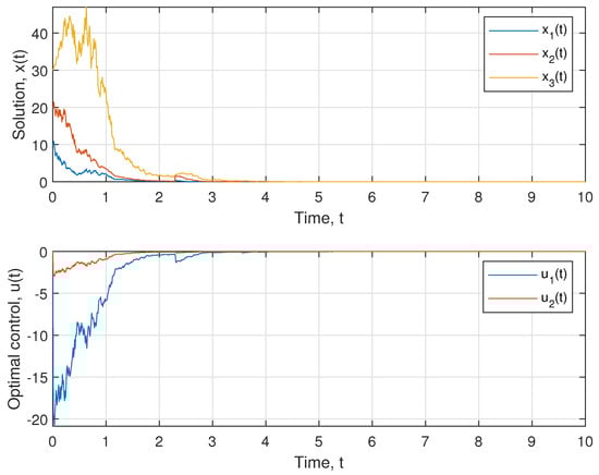
Figure 1. Realizations of the solution and optimal control with initial conditions $(10,20,30)$.

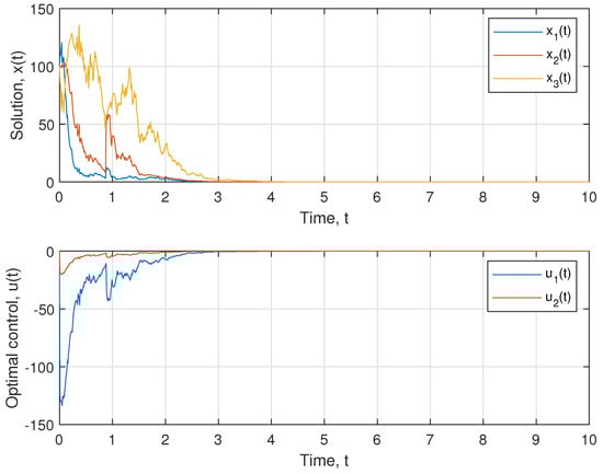
Figure 2. Realizations of solution and optimal control with initial conditions $(100,100,100)$.

As we can see from the above examples, the resulting optimal control, $u\left(t\right)$, stabilizes the system, and therefore minimizes the functional $I_u(y,h,x_0)$. In addition, considering the form of the matrix D from (42), we can see that $u_2\left(t\right)$ is close to 0, because

$$u^T\left(t\right)Du\left(t\right)=100u_1^2\left(t\right)+1600u_2^2\left(t\right).$$

In this way, the optimal control found will agree with the given quality functional $I_u(y,h,x_0)$.

An analysis of the solution showed that there is an optimal control for an arbitrary $\alpha \in [-1,1]$. The $\left|\alpha \right|<1$ case corresponds to the compressive case, since in this case the solution is compressed by the $\alpha$ coefficient at each step in the point, $t_k$. The $\left|\alpha \right|=1$ case is not compressible, but the existence of an optimal control can be found based on Theorem 3. The case of $\left|\alpha \right|>1$ is not included in the theory of this work, since in this case, the solution of Equation (50) either does not exist or is not positively defined. This case needs further investigation.

8. Discussion

In this work, we have obtained sufficient conditions for the existence of an optimal solution for a stochastic dynamical system with jumps, which transform the system to a stable one in probability. The second Lyapunov method was used to investigate the existence of an optimal solution. This method is efficient both for ordinary differential equations (ODE) and for stochastic differential equations (SDE). As it can be seen from the proof of the Theorem 2, the existence of finite bounds for jumps at non-random time moments, $t_m$ (${lim}_{m\to \infty }{t}_m=T^{*}<\infty$), does not impact the stability of the solution. On the other hand, $|t_{m+}-t_m|>\delta ,m\ge 1$ was used for proving the existence of the optimal control (Theorem 3). This restriction is also present in the works of other authors. Thus, a goal of future work could be to construct an optimal control without the assumption $|t_{m+}-t_m|>\delta ,m\ge 1$, which will considerably expand the scope of the second Lyapunov method.

The limitation of the proposed method is linked to the need for a solution to Riccati´s equations that can be computationally heavy. For small dimensions of m, Riccati′s equations can be solved either by iteration or by genetic algorithms, but for large dimensions of m, only genetic algorithms work.

9. Conclusions

In this work, we obtained sufficient conditions for the existence of a solution to an optimal stabilization problem for dynamical systems with jumps. We considered the case of a linear system with a quadratic quality functional. We showed that by designing an optimal control that stabilizes the system to a stable one in probability reduces the problem of solving the Riccati equations. Additionally, for a linear autonomous system, the method using a small parameter is substantiated for solving the problem of optimal stabilization. The obtained solutions can be used to describe a stock market in economics, biological systems, including models of response to treatment of cancer, and other complex dynamical systems.

In addition, this work serves as a basis for the study of systems of type (3)–(4) under the conditions of the presence of condensation point, i.e.,

$$\underset{k\to \infty }{lim}{t}_k=t^{*}<\infty .$$

Systems with this condition are a mathematical model of real phenomena, in which exceptional events accumulate very quickly over a finite period of time, which can lead to a collapse of the system. For example, paper [22] examines the mathematical model of the collapse of the bridge in Tacoma. At the same time, the authors of this work took into account only deterministic influences, and did not include random events affecting the dynamics of the bridge. Considering both deterministic and random influences can provide a more precise picture for the understanding of such dramatic effects.

References

- Kats, I.Y. Lyapunov Function Method in Problems of Stability and Stabilization of Random-Structure Systems; Izd. Uralsk. Gosakademii Putei Soobshcheniya: Yekaterinburg, Russia, 1998. (In Russian) [Google Scholar]
- Tsarkov, Y.F.; Yasinsky, V.K.; Malyk, I.V. Stability in impulsive systems with Markov perturbations in averaging scheme. 2. Averaging principle for impulsive Markov systems and stability analysis based on averaged equations. Cybern. Syst. Anal. 2011, 47, 44–54. [Google Scholar] [CrossRef]
- Oksendal, B. Stochastic Differential Equations; Springer: New York, NY, USA, 2013. [Google Scholar]
- Doob, J.L. Stochastic Processes; Wiley: New York, NY, USA, 1953. [Google Scholar]
- Jacod, J.; Shiryaev, A.N. Limit Theorems for Stochastic Processes. Vols. 1 and 2; Fizmatlit: Moscow, Russia, 1994. (In Russian) [Google Scholar]
- Lukashiv, T.O.; Yurchenko, I.V.; Yasinskii, V.K. Lyapunov function method for investigation of stability of stochastic Ito random-structure systems with impulse Markov switchings. I. General theorems on the stability of stochastic impulse systems. Cybern. Syst. Anal. 2009, 45, 281–290. [Google Scholar]
- Dynkin, E.B. Markov Processes; Academic Press: New York, NY, USA, 1965. [Google Scholar]
- Korolyuk, V.S.; Tsarkov, E.F.; Yasinskii, V.K. Probability, Statistics, and Random Processes. Theory and Computer Practice, Vol. 3, Random Processes. Theory and Computer Practice; Zoloti Lytavry: Chernivtsi, Ukraine, 2009. (In Ukrainian) [Google Scholar]
- Protter, P.E. Stochastic Integration and Differential Equations, 2nd ed.; Springer: New York, NY, USA, 2004. [Google Scholar]
- Koroliouk, V.S.; Samoilenko, I.V. Asymptotic expansion of a functional constructed from a semi-Markov random evolution in the scheme of diffusion approximation. Theory Probab. Math. Stat. 2018, 96, 83–100. [Google Scholar] [CrossRef]
- Tsarkov, Y.F.; Yasinsky, V.K.; Malyk, I.V. Stability in impulsive systems with Markov perturbations in averaging scheme. I. Averaging principle for impulsive Markov systems. Cybern. Syst. Anal. 2010, 46, 975–985. [Google Scholar] [CrossRef]
- Koroliuk, V.S.; Limnios, N. Stochastic Systems in Merging Phase Space; World Scientific Publishing Company: Singapore, 2005. [Google Scholar]
- Lukashiv, T.O.; Malyk, I.V. Stability of controlled stochastic dynamic systems of random structure with Markov switches and Poisson perturbations. Bukovinian Math. J. 2022, 10, 85–99. [Google Scholar] [CrossRef]
- Andreeva, E.A.; Kolmanovskii, V.B.; Shaikhet, L.E. Control of Hereditary Systems; Nauka: Moskow, Russia, 1992. (In Russian) [Google Scholar]
- Vadivel, R.; Ali, M.S.; Alzahranib, F. Robust H∞ synchronization of Markov jump stochastic uncertain neural networks with decentralized event-triggered mechanism. Chin. J. Phys. 2019, 60, 68–87. [Google Scholar] [CrossRef]
- Vadivel, R.; Hammachukiattikul, P.; Zhu, Q.; Gunasekaran, N. Event-triggered synchronization for stochastic delayed neural networks: Passivity and passification case. Asian J. Control. 2022. [Google Scholar] [CrossRef]
- Hasminsky, R.Z. Stability of Systems of Differential Equations under Random Parameter Perturbations; Nauka: Moscow, Russia, 1969. (In Russian) [Google Scholar]
- Skorokhod, A.V. Asymptotic Methods in the Theory of Stochastic Differential Equations; Naukova Dumka: Kyiv, Ukraine, 1987. (In Russian) [Google Scholar]
- Sverdan, M.L.; Tsar’kov, E.F. Stability of Stochastic Impulse Systems; RTU: Riga, Latvia, 1994. (In Russian) [Google Scholar]
- Kloeden, P.E.; Platen, E. Numerical Solution of Stochastic Differential Equations; Springer: Berlin, Germany, 1992. [Google Scholar]
- Lukashiv, T. One Form of Lyapunov Operator for Stochastic Dynamic System with Markov Parameters. J. Math. 2016, 2016, 1694935. [Google Scholar] [CrossRef]
- Arioli, G.; Gazzola, F. A new mathematical explanation of what triggered the catastrophic torsional mode of the Tacoma Narrows Bridge. Appl. Math. Model. 2015, 39, 901–912. [Google Scholar] [CrossRef]
Disclaimer/Publisher’s Note: The statements, opinions and data contained in all publications are solely those of the individual author(s) and contributor(s) and not of MDPI and/or the editor(s). MDPI and/or the editor(s) disclaim responsibility for any injury to people or property resulting from any ideas, methods, instructions or products referred to in the content. |
© 2023 by the authors. Licensee MDPI, Basel, Switzerland. This article is an open access article distributed under the terms and conditions of the Creative Commons Attribution (CC BY) license (https://creativecommons.org/licenses/by/4.0/).