Mean-Value-at-Risk Portfolio Optimization Based on Risk Tolerance Preferences and Asymmetric Volatility

Abstract

Investors generally aim to obtain a high return from their stock portfolio. However, investors must realize that a high value-at-risk (VaR) is essential to calculate for this aim. One of the objects in the VaR calculation is the asymmetric return volatility of stocks, which causes an unbalanced decrease and increase in returns. Therefore, this study proposes a mean-value-at-risk (mean-VaR) stock portfolio optimization model based on stocks’ asymmetric return volatility and investors’ risk aversion preferences. The first stage is the determination of the mean of all stocks in the portfolio conducted using the autoregressive moving average Glosten–Jagannathan–Runkle generalized autoregressive conditional heteroscedasticity (ARMA-GJR-GARCH) models. Then, the second stage is weighting the capital of each stock based on the mean-VaR model with the investors’ risk aversion preferences. This is conducted using the Lagrange multiplier method. Then, the model is applied to stock data in Indonesia’s capital market. This application also analyzed the sensitivity between the mean, VaR, both ratios, and risk aversion. This research can be used for investors in the design and weighting of capital in a stock portfolio to ensure its asymmetrical effect is as small as possible.

1. Introduction

An investment is an amount of money put down now in order to obtain benefits in the future [1]. Many people are highly interested in investing and invest in stocks. There are several important features concerning investment in stocks, namely, risk and return. The level of risk can be seen from the volatility of stock returns. The most frequently used model in a time series for financial problems is the generalized autoregressive conditional heteroscedasticity (GARCH) model introduced by Bollerslev [2]. The GARCH model has a more flexible structure to accommodate volatility in financial data [2]. However, the weakness of the GARCH model lies in capturing the asymmetry of good and bad news. Therefore, a study was conducted to overcome the asymmetric effects on the data by using the Glosten–Jagannatan–Runkle generalized autoregressive conditional heteroscedasticity (GJR-GARCH) model.

There are several previous studies, including that by Charles and Darné [3], which described a model that can overcome asymmetric effects, namely the GJR-GARCH model. The GJR-GARCH model is a development of GARCH by including leverage effects. Xu et al. [4] used the ARIMA-GJR-GARCH model to forecast the Renminbi (China’s currency) exchange rate against the Hong Kong dollar. The GJR-GARCH model can be used for asymmetric data in the variance equation. Based on the analysis in the paper, the ARIMA (1,1,1)-GJR-GARCH (1,1) model is the best model for exchange rates and forecasting. Su and Lin [5] determined value-at-risk using the GJR-GARCH model of financial ownership. The results obtained were that the GJR-GARCH model is good for VaR forecasting. Kalaychi et al. [6] conducted a comprehensive review of deterministic models and applications for portfolio optimization. Comprehensive survey results on deterministic models and applications are suggested for portfolio optimization. Al Janabi [7] examined the optimization of multivariate portfolios under illiquid market prospects. Based on that analysis, the portfolio manager can determine the closing horizon, and the dependencies of different sizes, and the LVaR calculations need to be performed to produce an investable portfolio. Aini & Lutfi [8] researched the effect of risk perception, risk tolerance, and loss aversion on investment decision-making. The results indicate that risk perception influences investment decision-making and risk tolerance. Pak and Mahmood [9] examined the impact of personality on risk tolerance and investment decisions. Based on these studies, personality traits have some effect on individual risk tolerance behaviors, thus influencing investment decisions in stocks, securities, and bonds.

Based on the research that has been described, there are still some deficiencies in these models. Among others, although Charles and Darné [3] and Xu et al. [4] used the GJR-GACH model to overcome asymmetric effects, they did not link it to investment portfolio optimization. Su and Lin [5] determined the VaR value using the GJR-GARCH model for financial holdings, but did not determine the mean-VaR investment portfolio. Kalayci et al. [6] and Al Janabi [7] applied portfolio optimization to determine models and determine portfolios that could be invested. However, the mean-VaR investment portfolio optimization model has not yet been determined, especially for stocks on the Indonesia Stock Exchange (IDX). Aini and Lutfi [8] and Pak and Mahmood [9] conducted research on risk tolerance, but did not apply it to several stocks. The current research is the mean-VaR investment portfolio optimization model based on risk tolerance preferences involving stocks that have asymmetric volatility. The method used is the autoregressive moving average (ARMA) to predict stock returns, and the Glosten, Jagannathan, and Runkle–generalized autoregressive conditional heteroscedasticity (GJR-GARCH) models to determine the risk level of asymmetry. Furthermore, portfolio risk is measured based on the value-at-risk (VaR) model, and the investment portfolio’s weight composition selection is based on the investor’s risk tolerance preference. The advantage of this study is that the determination of the mean-VaR is based on risk tolerance preferences involving stocks with asymmetric volatility. The usefulness of this research is that it can be used as a reference for investors as material for consideration in investing, especially in the ten stocks analyzed.

2. The Mechanism Framework

2.1. Autoregressive-Moving-Average (ARMA) Model

Suppose that there are $T$ days considered in the sampling process. Daily closing stock return at day $t,$ $\{r_t:t=1,2,\dots ,T\}$, is assumed as a stationary random sequence in mean and variance, that is as follows [10,11]:

$$E\left(r_t\right)=\mu \mathrm{and}Var\left(r_t\right)={\sigma }^2.$$

The sample value of $r_t$ is calculated using the equation as follows [12]:

$$r_t=\mathit{ln}\frac{P_t}{P_{t-1}},$$

(1)

where $P_t$ represents the daily closing stock price at day $t$. The daily closing stock return today in the ARMA model is assumed to be dependent on itself and its error in previous days [13]. Mathematically, the ARMA model with autoregressive order $p$ and moving-average order $q$, denoted as ARMA ($p$, $q$), for $r_t$ is expressed in the following equation [14]:

$$r_t={\varphi }_0+\sum _{i=1}^p{\varphi }_i{r}_{t-i}-\sum _{j=1}^q{\theta }_j{\epsilon }_{t-j}+{\epsilon }_t,$$

(2)

where $\{{\epsilon }_t:t=1,2,\dots ,T\}$ represents random error sequences assumed to be independent and identically normally distributed with zero mean and constant variance, ${\varphi }_0$ represents constant parameter, ${\varphi }_i$ with $i=1,2,\dots ,p$ represents $i$-th autoregressive parameter, and ${\theta }_j$ with $j=1,2,\dots ,q$ represents $j$-th moving-average parameter. By using the backshift operator, Equation (2) can be written as follows [15]:

$$\left(1-{\varphi }_{1}B-...-{\varphi }_p{B}^p\right)r_t={\varphi }_0+\left(1-{\theta }_{1}B-...-{\theta }_q{B}^q\right){\epsilon }_t.$$

where $B$ represents backshift operator, e.g., $B{r}_t=r_{t-1}$, $B^2{r}_t=r_{t-2}$, …, $B^p{r}_t=r_{t-p}$, $B{\epsilon }_t={\epsilon }_{t-1}$, $B^2{\epsilon }_t={\epsilon }_{t-2}$, …, and $B^q{\epsilon }_t={\epsilon }_{t-q}$.

2.2. Glosten–Jagannathan–Runkle–Generalized Autoregressive Conditional Heteroscedasticity (GJR-GARCH) Model

The volatility, another word for the variance, of the random error ${\epsilon }_t$ in Equation (2) can be nonconstant. For this case, Bollerslev [2] formulated ${\epsilon }_t$ with nonconstant variance as follows:

$${\epsilon }_t={\sigma }_t{u}_t,$$

where $\left\{u_t:t=1,2,\dots ,T\right\}$ epresents an independent and identically normally distributed random variable sequence with mean 0 and variance 1. In more detail, $\left\{u_t\right\}$ and $\left\{{\epsilon }_t\right\}$ are independent. The volatility of today’s random error can be assumed to depend on itself and the random error in previous days. Mathematically, it is expressed as follows [5]:

$${\sigma }_t^2={\alpha }_0+\sum _{k=1}^r{\alpha }_k{\epsilon }_{t-k}^2+\sum _{l=1}^s{\beta }_l{\sigma }_{t-l}^2,$$

(3)

where ${\sigma }_t^2$ is variance of ${\epsilon }_t$, ${\alpha }_0$ represents the constant parameter, ${\alpha }_k$ with $k=1,2,\dots ,r$ represents the ${\epsilon }_{t-k}$’s autoregressive parameter, ${\beta }_l$ with $l=1,2,\dots ,s$ represents the autoregressive parameter of ${\sigma }_{t-l}^2$. The Equation (3) is better known as a generalized autoregressive conditional heteroscedasticity (GARCH) model with volatility’s autoregressive order $r$ and random error’s autoregressive order $s$, GARCH ($r$, $s$). There are limits to the parameters to guarantee that ${\sigma }_t^2$ in Equation (2) is positive. These limitations are as follows [5]:

$${\alpha }_0>0,{\alpha }_k\ge 0,{\beta }_l\ge 0,\mathrm{and}{\sum }_{k=1}^r{\alpha }_k+{\sum }_{l=1}^s{\beta }_s<1.$$

(4)

The volatility of ${\epsilon }_t$ may not only suffer from inconstancy, but it may also suffer from asymmetry. In other words, the volatility values below and above the zero line (${\epsilon }_t$’s mean line) are not balanced. It may also generally occur in stock return data, where increases and decreases are often unbalanced. If this is not addressed, then the volatility of stock returns will be extreme at one sign and the opposite at another. It can cause returns from forecasting in the ARMA model to be spurious [16]. The inconstancy and asymmetry of the volatility ${\epsilon }_t$ can be overcome by using the Glosten–Jagannathan–Runkle–generalized autoregressive conditional heteroscedasticity (GJR-GARCH) model. The general form of the GJR-GARCH ($r$, $s$, $v$) model is expressed as follows [16]:

$${\sigma }_t^2={\alpha }_0+\sum _{k=1}^r{\alpha }_k{\epsilon }_{t-k}^2+\sum _{l=1}^s{\beta }_l{\sigma }_{t-l}^2+{\sum }_{m=1}^v{\gamma }_m{\epsilon }_{t-k}{1}_{t-k}^{+},$$

(5)

where ${\gamma }_m$ with $m=1,2,\dots ,v$ represents the $m$-th parameter leverage effect, and

$$1_{t-k}^{+}=\left\{\begin{array}{cc}1& :{\epsilon }_{t-k}>0\\ 0& :{\epsilon }_{t-k}\le 0\end{array}\right..$$

(6)

${\gamma }_m$, which has positive and negative values, will add to and decrease the predicted value of today’s volatility to adjust for the influence of asymmetric volatility [3,17].

2.3. Statistical Tests

This section briefly explains the statistical tests used in the study. These statistical tests include stationarity tests, model significance tests, distribution fit tests, independence tests, heteroscedasticity tests, and asymmetry tests.

2.3.1. Stationarity Test

The data stationarity test used in this research is the Dicky–Fuller (DF) test. The null hypothesis is $H_0:{\widehat{\varphi }}_1=1$, meaning the data is stationary. Therefore, the alternative is $H_1:{\widehat{\varphi }}_1<1$, meaning that data is not stationary [18]. The statistical value of this test is calculated as follows:

$$D{F}_{test}=\frac{{\widehat{\varphi }}_1-1}{{\sigma }_{{\widehat{\varphi }}_1}},$$

(7)

where ${\widehat{\varphi }}_1$ represents the estimate of the first autoregressive parameter of ARMA (1, 0), and ${\sigma }_{{\widehat{\varphi }}_1}$ represents the standard deviation of ${\widehat{\varphi }}_1$. Reject $H_0$ if $D{F}_{test}$ is greater than the absolute critical value at the significant level $\kappa$, $t_{\kappa }$, and vice versa [19].

2.3.2. Distribution Fit Test

The distribution fit test in this study was carried out using the Kolmogorov–Smirnov (KS) test. The null hypothesis ($H_0$) in this test states that there is a fitness between the data distribution and the theoretical one, whereas the alternative hypothesis ($H_0$) states the inverse of it [20]. The statistical value of this test is calculated as follows [21]:

$${KS}_{test}=\sup \left\{F_{r_t}\left(r\right)-F_e\left(r\right):r\in r_t\right\},$$

(8)

where ${\widehat{r}}_t$ represents $r_t$’s forecast. Reject $H_0$ if ${KS}_{test}$ is greater that its critical value with significant level $\kappa$, $K{S}_{\kappa }$, and vice versa.

2.3.3. Independence Test

The independence test in this study was carried out using the Ljung–Box (LB) test. The null hypothesis ($H_0$) in this test states that the data are independent of each other, whereas the alternative hypothesis ($H_1$) states the inverse of it. The statistical value of this test is calculated as follows [22]:

$${LB}_{test}=T(T+2)\sum _{m=1}^M\frac{h_m^2}{T-m},$$

(9)

where $M$ represents the optimal lag, and $h_m$ is calculated using the following equation:

$$h_m=\frac{\sum _{t=m+1}^T{\epsilon }_t{\epsilon }_{t-m}}{\sum _{t=1}^T{\epsilon }_t^2}.$$

Reject $H_0$ if ${LB}_{test}$ is greater that its critical value with significant level $\kappa$, ${LB}_{\kappa }$, and vice versa.

2.3.4. Heteroscedasticity Test

The heteroscedasticity test in this study was carried out using the Glejser test. The first step is estimating the parameters ${\zeta }_0$ and ${\zeta }_1$ in the following regression equation [23]:

$$\left|{\epsilon }_t\right|={\zeta }_0+{\zeta }_1{r}_t.$$

(10)

Second, determine the null and alternative hypotheses. The null hypothesis in this test is $H_0:{\mathsf{\zeta }}_1=0$, meaning heteroscedasticity exists in the sample error ${\epsilon }_t$. Then, the alternative hypothesis is $H_1:{\mathsf{\zeta }}_1\ne 0$, meaning there is no heteroscedasticity in the sample error ${\epsilon }_t$. Third, determine the significance of the parameter ${\zeta }_1$1 using a t-test. Finally, reject $H_0$ if $\left|T_{test}\right|$ is greater than the absolute of its critical value with a significant level $\kappa$ and degree of freedom $T-1$, $\left|t_{\frac{\kappa }{2},T-1}\right|$, and vice versa [24].

2.3.5. Asymmetry Test

The asymmetry test in this study was carried out using the cross-correlation (CC) test. The first step is estimating the parameters ${ϵ}_0$, ${ϵ}_1$, ${ϵ}_2$, and ${ϵ}_3$ in the following regression equation:

$${\epsilon }_t^2={ϵ}_0+{ϵ}_1{1}_{t-1}^{-}+{ϵ}_2{\epsilon }_{t-1}{1}_{t-1}^{-}+{ϵ}_3{\epsilon }_{t-1}{1}_{t-1}^{+},$$

(11)

where

$$1_{t-k}^{-}=\left\{\begin{array}{cc}1& :{\epsilon }_{t-k}<0\\ 0& :{\epsilon }_{t-k}\ge 0\end{array}\right.,$$

and $1_{t-1}^{+}$ is expressed in Equation (6). Second, determine the null and alternative hypotheses. The null hypothesis in this test is $H_0:{ϵ}_0={ϵ}_1={ϵ}_2={ϵ}_3=0$, meaning that the error ${\epsilon }_t$ is symmetric. Then, the alternative hypothesis is $H_1:\exists {ϵ}_{\mathrm{y}}\ne 0$ with $y=0,1,2,3$, meaning that the error ${\epsilon }_t$ is asymmetric. Third, determine the statistical test using this formula as follows:

$$G_{test}=2\sum _{t=1}^T\left|{\epsilon }_t\right|\ln \frac{\left|{\epsilon }_t\right|}{\left|{\widehat{\epsilon }}_t\right|},$$

(12)

Finally, reject $H_0$ if $G_{test}$ is greater than its critical value with significant level $\kappa$ and degree of freedom $g,$ ${\chi }_{\kappa ,g}^2$, and vice versa.

2.4. Mean-Value-at-Risk (Mean-VaR) Portfolio Optimization Model with Investor’s Risk Tolerance

Portfolio optimization involves balancing reward and risk in financial assets [25,26,27]. The classical mean-variance model is used for portfolio selection, but its asymmetric distributions and excess kurtosis have led to criticism of variance as a risk measure [28,29,30,31]. Markowitz suggested a semi-variance risk measure to measure variability below the mean. Realistic risk measures like value-at-risk (VaR) and expected shortfall or conditional value-at-risk (CVAR) are used to separate undesirable downside and upside movements [32]. Rockafellar and Uryasev [33] discussed VAR and CVaR with regular distributions, focusing on mathematical properties, stability, simplicity, and acceptance. Despite their limitations, VaR is widely adopted in the financial industry but faces computational challenges [34,35].

Suppose there are $N$ stocks in stock portfolio $P$. The return from each stock is assumed to be normally distributed with its mean and variance [36]. The expected total return of portfolio $P$, denoted by ${\mu }_P$, is expressed as follows:

$${\mu }_P=\sum _{n=1}^N{w}_n{\mu }_n={\mathbf{w}}^T\mathsf{\mu }.$$

(13)

where $w_n$ with $n=1,2,\dots ,N$ represents the capital weight of the nth stock, ${\mu }_n$ with $n=1,2,\dots ,N$ represents the mean of return of the nth stock. In more detail, $\mathbf{w}$ and $\mathsf{\mu }$ each represent vectors of size $N\times 1$ which are expressed as follows:

$$\mathbf{w}=\left[\begin{array}{c}{w}_1\\ w_2\\ ⋮\\ w_N\end{array}\right] \mathrm{a}\mathrm{n}\mathrm{d} \mathsf{\mu }=\left[\begin{array}{c}{\mu }_1\\ {\mu }_2\\ ⋮\\ {\mu }_N\end{array}\right].$$

It must be noted that the total weight of the assets in the portfolio $P$ is 1. It can be mathematically written as follows:

$$\sum _{n=1}^N{w}_n={\mathbf{w}}^T\mathbf{e}=1,$$

(14)

where $\mathbf{e}$ represents a vector of size $N\times 1$, which is expressed as follows:

$$\mathbf{e}=\left[\begin{array}{c}1\\ 1\\ ⋮\\ 1\end{array}\right].$$

Meanwhile, the value-at-risk (VaR) of the portfolio $P$, used to measure the maximum potential loss of it [31,32], is expressed as follows [33,34]:

$$Va{R}_P\left(\alpha \right)=-\left\{{\mathbf{w}}^T\mathsf{\mu }+z_{\alpha }{\left({\mathbf{w}}^T\mathsf{\Sigma }\mathbf{w}\right)}^{\frac{1}{2}}\right\},$$

(15)

where $z_{\alpha }$ represents the ($1-\alpha$)-th percentile of the standard normal distribution, and $\mathsf{\Sigma }$ is an $N\times N$ matrix that represents the covariance matrix of the returns of $N$ stocks in the portfolio. The value of $\alpha$ can be adjusted according to the investor’s preferences. The greater the value of $\alpha$, the smaller the maximum loss from the investment portfolio preferences by the investor, and vice versa. VaR in Equation (15) is determined based on the standard deviation rule.

In the face of maximum loss from the portfolio, investors have different risk tolerances. Risk tolerance is the investors’ tendency to accept loss uncertainty in their investments. In other words, the bigger the investor’s risk tolerance, the more courageous the investor is to face uncertainty. Mathematically, risk tolerance is expressed as follows:

$$\tau =\frac{2}{\rho },$$

(16)

where $\rho$ represents the risk aversion [33].

The mean-VaR portfolio optimization model considering risk tolerance is formulated as follows [37,38]:

$$\begin{array}{cc}max.\tau {\mu }_P+Va{R}_P\left(\alpha \right)& =\tau {\mathbf{w}}^T\mathsf{\mu }+\left[-\left\{{\mathbf{w}}^T\mathsf{\mu }+z_{\alpha }{\left({\mathbf{w}}^T\mathsf{\Sigma }\mathbf{w}\right)}^{\frac{1}{2}}\right\}\right]\\ & =(\tau -1){\mathbf{w}}^T\mathsf{\mu }-z_{\alpha }{\left({\mathbf{w}}^T\mathsf{\Sigma }\mathbf{w}\right)}^{\frac{1}{2}}\hfill \\ \mathrm{s}.\mathrm{t}.{\mathbf{e}}^T\mathbf{w}=1,\mathbf{w}\ge 0.& \end{array}$$

(17)

The Lagrange multiplier method can be used to determine the solution of the model in Equation (17). It is explained in detail in Theorem 1. However, the solution stated in Theorem 1 may not satisfy the necessary condition as a global maximum solution.

Theorem 1.

If the mean-VaR portfolio optimization problem with risk tolerance, such as Equation (17), is solved using the Lagrange multiplier method, the solution is expressed as follows:

$$\mathbf{w}=\frac{{\mathsf{\Sigma }}^{-1}\left[\left(\tau -1\right)\mathsf{\mu }+\lambda \mathbf{e}\right]}{{\mathbf{e}}^T{\mathsf{\Sigma }}^{-1}\left[\left(\tau -1\right)\mathsf{\mu }+\lambda \mathbf{e}\right]},$$

(18)

where$\lambda$represents Lagrangian multiplier as follows:

$$\lambda =\frac{-\mathcal{a}\pm \sqrt{{\mathcal{b}}^2-4\mathcal{a}\mathcal{c}}}{2\mathcal{a}}:\lambda >0,$$

(19)

where$\mathcal{a}={\mathit{e}}^T{\mathit{\Sigma }}^{-1}\mathit{e},$$\mathcal{b}=2\left(\tau -1\right)$, and$\mathcal{c}=-z_{\alpha }^2+{\left(\tau -1\right)}^2{\mathit{\mu }}^T{\mathit{\Sigma }}^{-1}\mathit{\mu }$.

Proof. 

The Lagrange multiplier equation for the model Equation (17) can be expressed as follows [8,18]:

$$\mathcal{L}\left(\mathbf{w},\lambda \right)=\left(\tau -1\right){\mathbf{w}}^T\mathsf{\mu }-z_{\alpha }{\left({\mathbf{w}}^T\mathsf{\Sigma }\mathbf{w}\right)}^{\frac{1}{2}}+\lambda ({\mathbf{e}}^T\mathbf{w}-1).$$

(20)

The solution to Equation (20) is the zero maker of Equation (20) as follows:

$$\frac{\partial }{\partial \mathbf{w}}\mathcal{L}\left(\mathbf{w},\lambda \right)=\left(\tau -1\right)\mathsf{\mu }-z_{\alpha }\frac{\mathsf{\Sigma }\mathbf{w}}{{\left({\mathbf{w}}^T\mathsf{\Sigma }\mathbf{w}\right)}^{\frac{1}{2}}}+\lambda \mathbf{e}=0,$$

(21)

and

$$\frac{\partial }{\partial \lambda }\mathcal{L}\left(\mathbf{w},\lambda \right)={\mathbf{e}}^T\mathbf{w}-1=0.$$

(22)

The vector $\mathbf{w}$ is determined first. Multiply both sides of Equation (21) by $\frac{1}{z_{\alpha }}{\left({\mathbf{w}}^T\mathsf{\Sigma }\mathbf{w}\right)}^{\frac{1}{2}}{\mathsf{\Sigma }}^{-1}$ from the left so that this results in the following equation:

$$\frac{\left(\tau -1\right)}{z_{\alpha }}{\left({\mathbf{w}}^T\mathsf{\Sigma }\mathbf{w}\right)}^{\frac{1}{2}}{\mathsf{\Sigma }}^{-1}\mathsf{\mu }-\mathbf{w}+\frac{\lambda }{z_{\alpha }}{\left({\mathbf{w}}^T\mathsf{\Sigma }\mathbf{w}\right)}^{\frac{1}{2}}{\mathsf{\Sigma }}^{-1}\mathbf{e}=0.$$

$$\frac{1}{z_{\alpha }}{\left({\mathbf{w}}^T\mathsf{\Sigma }\mathbf{w}\right)}^{\frac{1}{2}}{\mathsf{\Sigma }}^{-1}\left[\left(\tau -1\right)\mathsf{\mu }+\lambda \mathbf{e}\right]-\mathbf{w}=0.$$

(23)

Then, multiply both sides of Equation (23) by ${\mathbf{e}}^T$ from the left so that this results in the following equation:

$$\frac{1}{z_{\alpha }}{\left({\mathbf{w}}^T\mathsf{\Sigma }\mathbf{w}\right)}^{\frac{1}{2}}{\mathbf{e}}^T{\mathsf{\Sigma }}^{-1}\left[\left(\tau -1\right)\mathsf{\mu }+\lambda \mathbf{e}\right]-{\mathbf{e}}^T\mathbf{w}={\mathbf{e}}^{T}0,$$

$$\frac{1}{z_{\alpha }}{\left({\mathbf{w}}^T\mathsf{\Sigma }\mathbf{w}\right)}^{\frac{1}{2}}{\mathbf{e}}^T{\mathsf{\Sigma }}^{-1}\left[\left(\tau -1\right)\mathsf{\mu }+\lambda \mathbf{e}\right]-1=0,$$

$${\left({\mathbf{w}}^T\mathsf{\Sigma }\mathbf{w}\right)}^{\frac{1}{2}}=\frac{z_{\alpha }}{{\mathbf{e}}^T{\mathsf{\Sigma }}^{-1}\left[\left(\tau -1\right)\mathsf{\mu }+\lambda \mathbf{e}\right]}.$$

(24)

Substitute Equation (24) into Equation (23) so that this results in the following equation:

$$\frac{{\mathsf{\Sigma }}^{-1}\left[\left(\tau -1\right)\mathsf{\mu }+\lambda \mathbf{e}\right]}{{\mathbf{e}}^T{\mathsf{\Sigma }}^{-1}\left[\left(\tau -1\right)\mathsf{\mu }+\lambda \mathbf{e}\right]}-\mathbf{w}=0,$$

$$\mathbf{w}=\frac{{\mathsf{\Sigma }}^{-1}\left[\left(\tau -1\right)\mathsf{\mu }+\lambda \mathbf{e}\right]}{{\mathbf{e}}^T{\mathsf{\Sigma }}^{-1}\left[\left(\tau -1\right)\mathsf{\mu }+\lambda \mathbf{e}\right]}.$$

(25)

Next, the determination of the solution $\lambda$. Multiply both sides of Equation (25) by ${\mathbf{w}}^T\mathsf{\Sigma }$ so that this results in the following equation:

$${\mathbf{w}}^T\mathsf{\Sigma }\mathbf{w}=\frac{{\mathbf{w}}^T\mathsf{\Sigma }{\mathsf{\Sigma }}^{-1}\left[\left(\tau -1\right)\mathsf{\mu }+\lambda \mathbf{e}\right]}{{\mathbf{e}}^T{\mathsf{\Sigma }}^{-1}\left[\left(\tau -1\right)\mathsf{\mu }+\lambda \mathbf{e}\right]},$$

$${\mathbf{w}}^T\mathsf{\Sigma }\mathbf{w}=\frac{{\mathbf{w}}^T\left[\left(\tau -1\right)\mathsf{\mu }+\lambda \mathbf{e}\right]}{{\mathbf{e}}^T{\mathsf{\Sigma }}^{-1}\left[\left(\tau -1\right)\mathsf{\mu }+\lambda \mathbf{e}\right]}.$$

(26)

Substitute Equation (24) into Equation (26),

$${\left\{\frac{z_{\alpha }}{{\mathbf{e}}^T{\mathsf{\Sigma }}^{-1}\left[\left(\tau -1\right)\mathsf{\mu }+\lambda \mathbf{e}\right]}\right\}}^2=\frac{{\mathbf{w}}^T\left[\left(\tau -1\right)\mathsf{\mu }+\lambda \mathbf{e}\right]}{{\mathbf{e}}^T{\mathsf{\Sigma }}^{-1}\left[\left(\tau -1\right)\mathsf{\mu }+\lambda \mathbf{e}\right]},$$

$$\frac{z_{\alpha }^2}{{\mathbf{e}}^T{\mathsf{\Sigma }}^{-1}\left[\left(\tau -1\right)\mathsf{\mu }+\lambda \mathbf{e}\right]}={\mathbf{w}}^T\left[\left(\tau -1\right)\mathsf{\mu }+\lambda \mathbf{e}\right].$$

(27)

Substitute Equation (25) into Equation (27),

$$\frac{z_{\alpha }^2}{{\mathbf{e}}^T{\mathsf{\Sigma }}^{-1}\left[\left(\tau -1\right)\mathsf{\mu }+\lambda \mathbf{e}\right]}={\left[\left(\tau -1\right)\mathsf{\mu }+\lambda \mathbf{e}\right]}^T\frac{{\mathsf{\Sigma }}^{-1}\left[\left(\tau -1\right)\mathsf{\mu }+\lambda \mathbf{e}\right]}{{\mathbf{e}}^T{\mathsf{\Sigma }}^{-1}\left[\left(\tau -1\right)\mathsf{\mu }+\lambda \mathbf{e}\right]},$$

$$z_{\alpha }^2=\left[\left(\tau -1\right){\mathsf{\mu }}^T+\lambda {\mathbf{e}}^T\right]\left[\left(\tau -1\right){\mathsf{\Sigma }}^{-1}\mathsf{\mu }+\lambda {\mathsf{\Sigma }}^{-1}\mathbf{e}\right],$$

$$0=-z_{\alpha }^2+{\left(\tau -1\right)}^2{\mathsf{\mu }}^T{\mathsf{\Sigma }}^{-1}\mathsf{\mu }+\left(\tau -1\right)\lambda {\mathsf{\mu }}^T{\mathsf{\Sigma }}^{-1}\mathbf{e}+\lambda \left(\tau -1\right){\mathbf{e}}^T{\mathsf{\Sigma }}^{-1}\mathsf{\mu }+{\lambda }^2{\mathbf{e}}^T{\mathsf{\Sigma }}^{-1}\mathbf{e},$$

$$0=-z_{\alpha }^2+{\left(\tau -1\right)}^2{\mathsf{\mu }}^T{\mathsf{\Sigma }}^{-1}\mathsf{\mu }+2\lambda \left(\tau -1\right)+{\lambda }^2{\mathbf{e}}^T{\mathsf{\Sigma }}^{-1}\mathbf{e}.$$

(28)

Equation (28) is a quadratic equation, so the possible values of $\lambda$ are as follows:

$$\lambda =\frac{-\mathcal{a}\pm \sqrt{{\mathcal{b}}^2-4\mathcal{a}\mathcal{c}}}{2\mathcal{a}}:\lambda >0,$$

(29)

where $\mathcal{a}={\mathbf{e}}^T{\mathsf{\Sigma }}^{-1}\mathbf{e}$, $\mathcal{b}=2\left(\tau -1\right)$, and $\mathcal{c}=-z_{\alpha }^2+{\left(\tau -1\right)}^2{\mathsf{\mu }}^T{\mathsf{\Sigma }}^{-1}\mathsf{\mu }$. □

The solution $\mathbf{w}$ in Equation (20) given in Theorem 1 may fulfil the necessary conditions as a global maximum solution [39,40]. The solution $\mathbf{w}$ is called the global maximum solution of Equation (20) if this condition is satisfied:

$$\forall \mathbf{x}\in {\mathbb{R}}^{N+1}-\left\{0\right\},{\mathbf{x}}^T\mathbf{H}\left(\mathbf{w},\lambda \right)\mathbf{x}<0,$$

(30)

where $\mathbf{H}\left(\mathbf{w},\lambda \right)$ represents the Hessian matrix of Equation (20) as follows:

$$\mathbf{H}\left(\mathbf{w},\lambda \right)=\left[\begin{array}{cc}\frac{{\partial }^{2}L\left(\mathbf{w},\lambda \right)}{\partial {\mathbf{w}}^2}& \frac{{\partial }^{2}L\left(\mathbf{w},\lambda \right)}{\partial \mathbf{w}\partial \lambda }\\ \frac{{\partial }^{2}L\left(\mathbf{w},\lambda \right)}{\partial \lambda \partial \mathbf{w}}& \frac{\partial L\left(\mathbf{w},\lambda \right)}{\partial {\lambda }^2}\end{array}\right]=\left[\begin{array}{cc}{z}_{\alpha }\left\{\frac{\mathsf{\Sigma }}{{\left({\mathbf{w}}^T\mathsf{\Sigma }\mathbf{w}\right)}^{\frac{1}{2}}}-\frac{\mathsf{\Sigma }\mathbf{w}{\mathbf{w}}^T\mathsf{\Sigma }}{{\left({\mathbf{w}}^T\mathsf{\Sigma }\mathbf{w}\right)}^{\frac{3}{2}}}\right\}& \mathbf{e}\\ {\mathbf{e}}^T& 0\end{array}\right].$$

(31)

3. Application of Mechanism

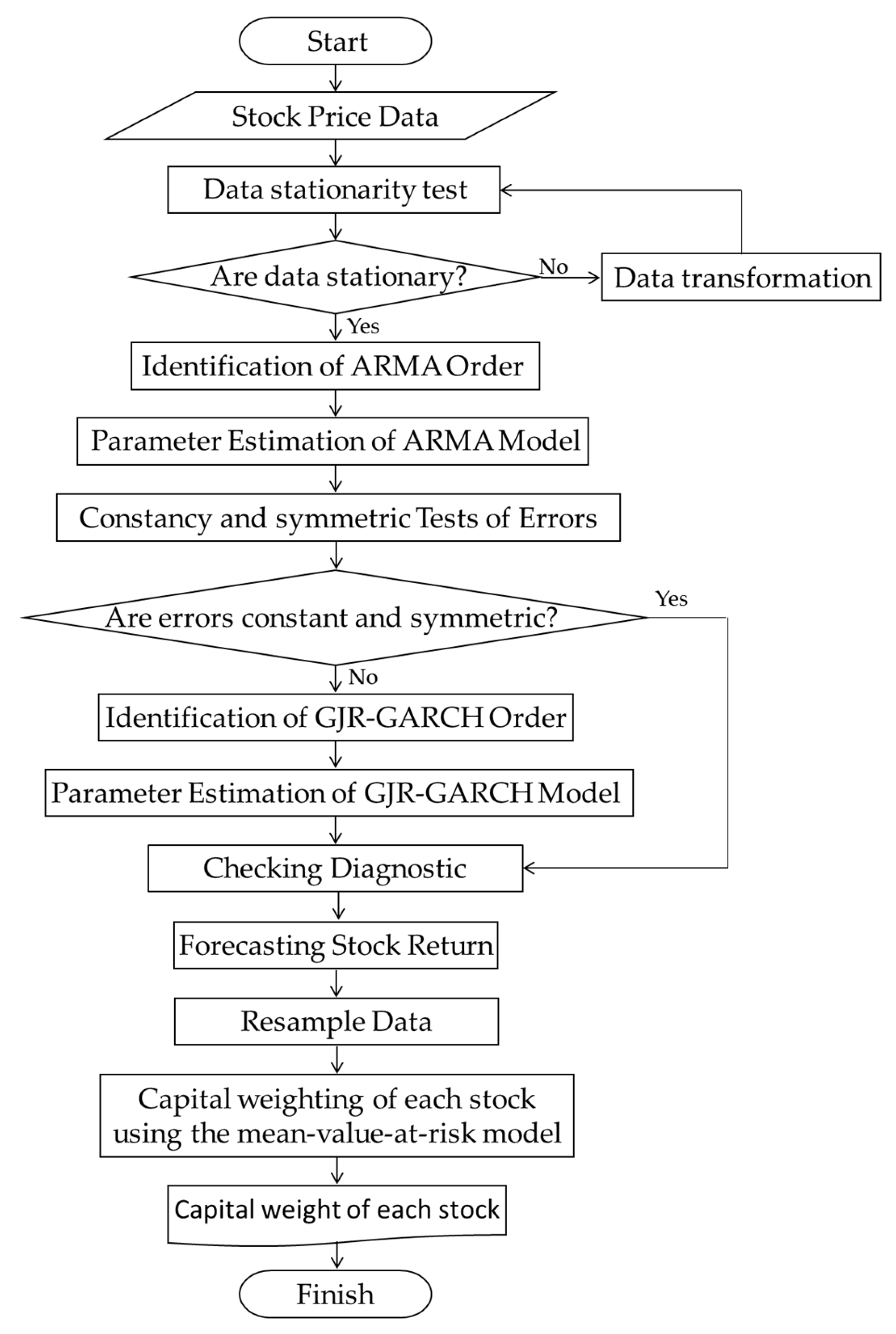
3.1. Algorithm to Apply Mechanism on Real Data

The mechanism framework discussed in Section 2.2 is experimented on real data. The algorithm is as follows:

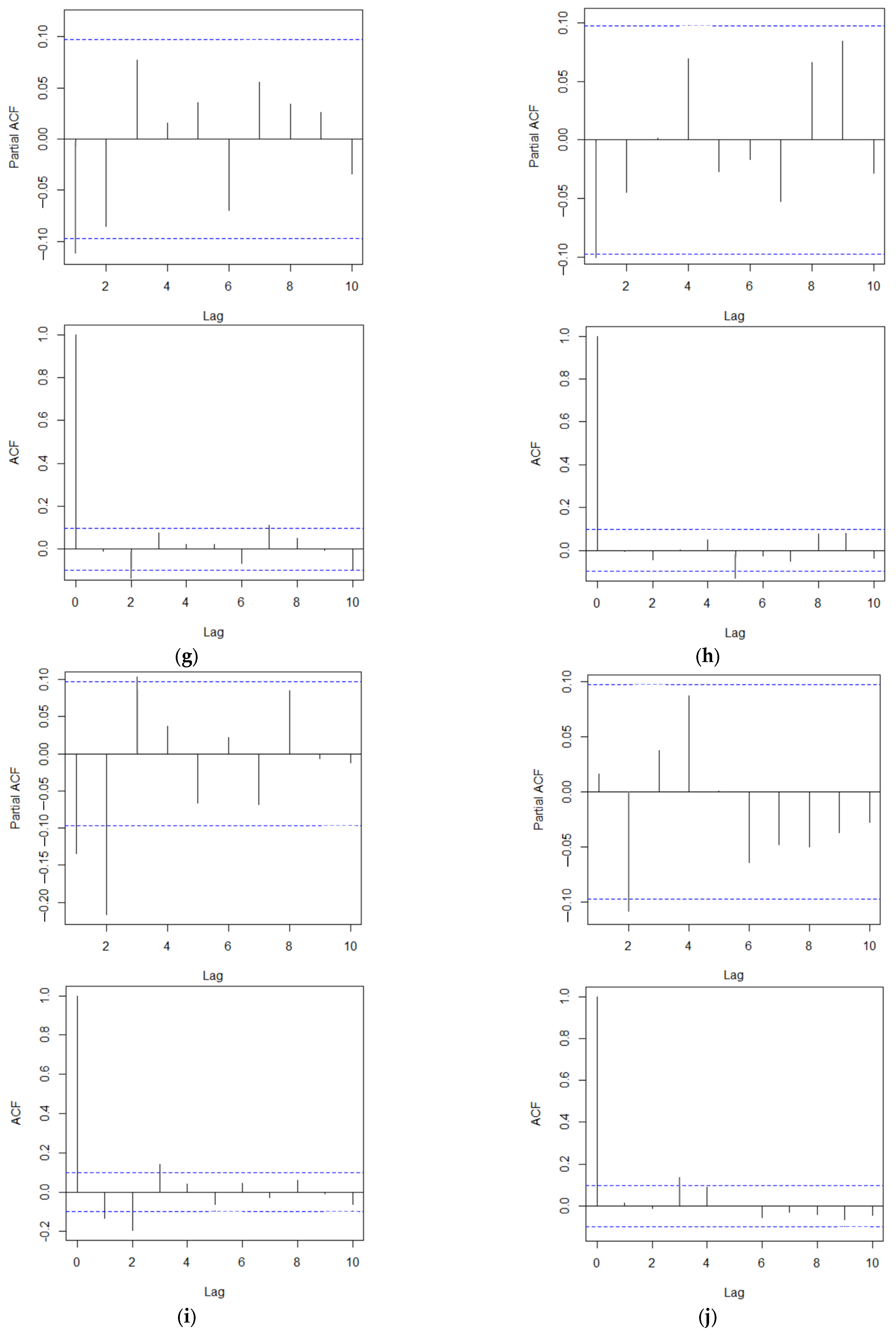
• Check the stationarity of each return data for each stock. The examination in this study was carried out using the Dicky–Fuller test (see Section 2.3.1). If the data is stationary, the experiment continues to the next stage, whereas if vice versa, the data is transformed first, e.g., into logarithmic form and data differentiation transformation.
  Identify orders from the ARMA model. Identification of AR and MA orders in this research is carried out using partial-autocorrelation and auto-correlation function diagrams, respectively.
• Estimate the parameters of the ARMA model. This assessment in this study was carried out using the maximum likelihood (ML) method.
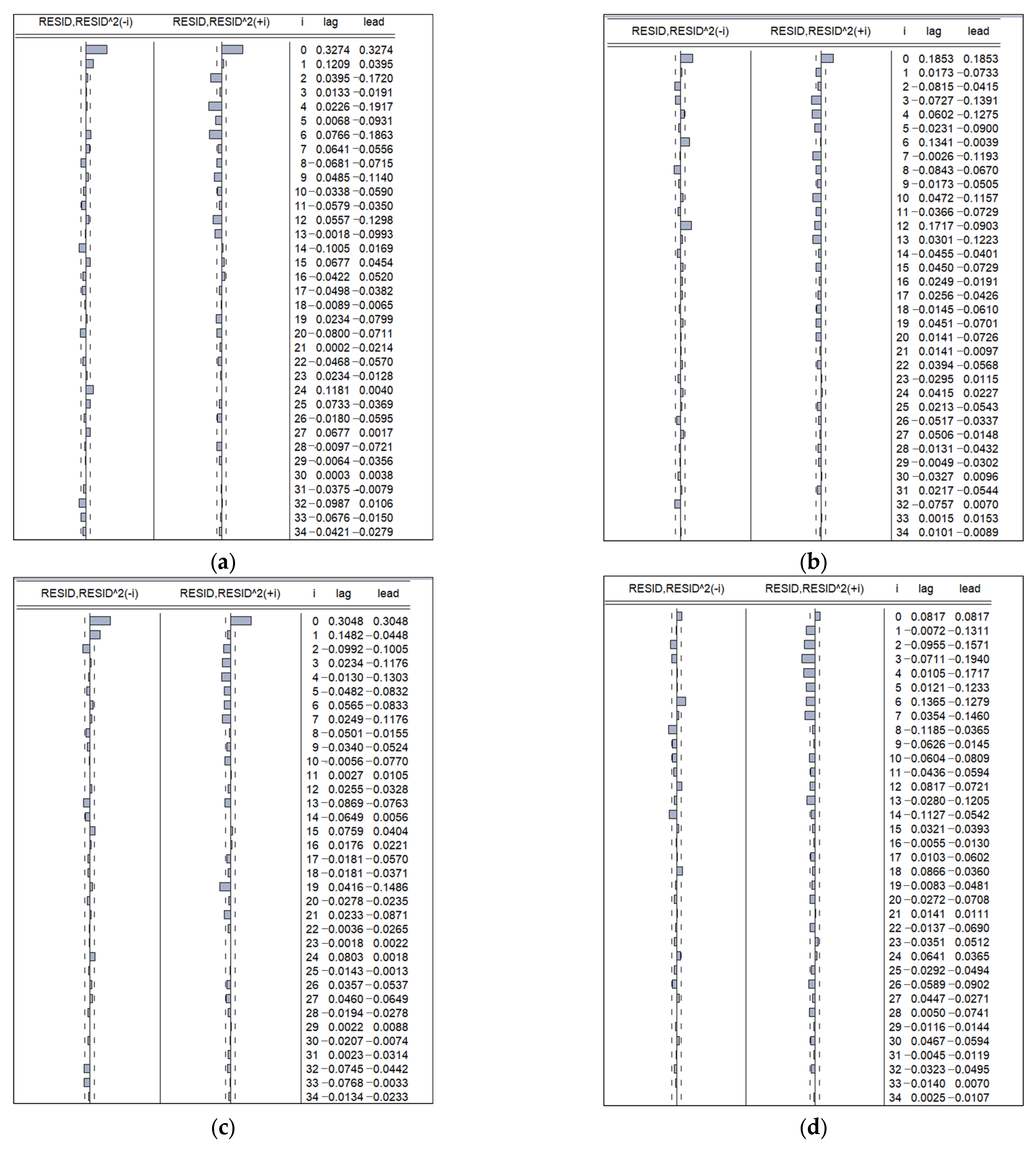
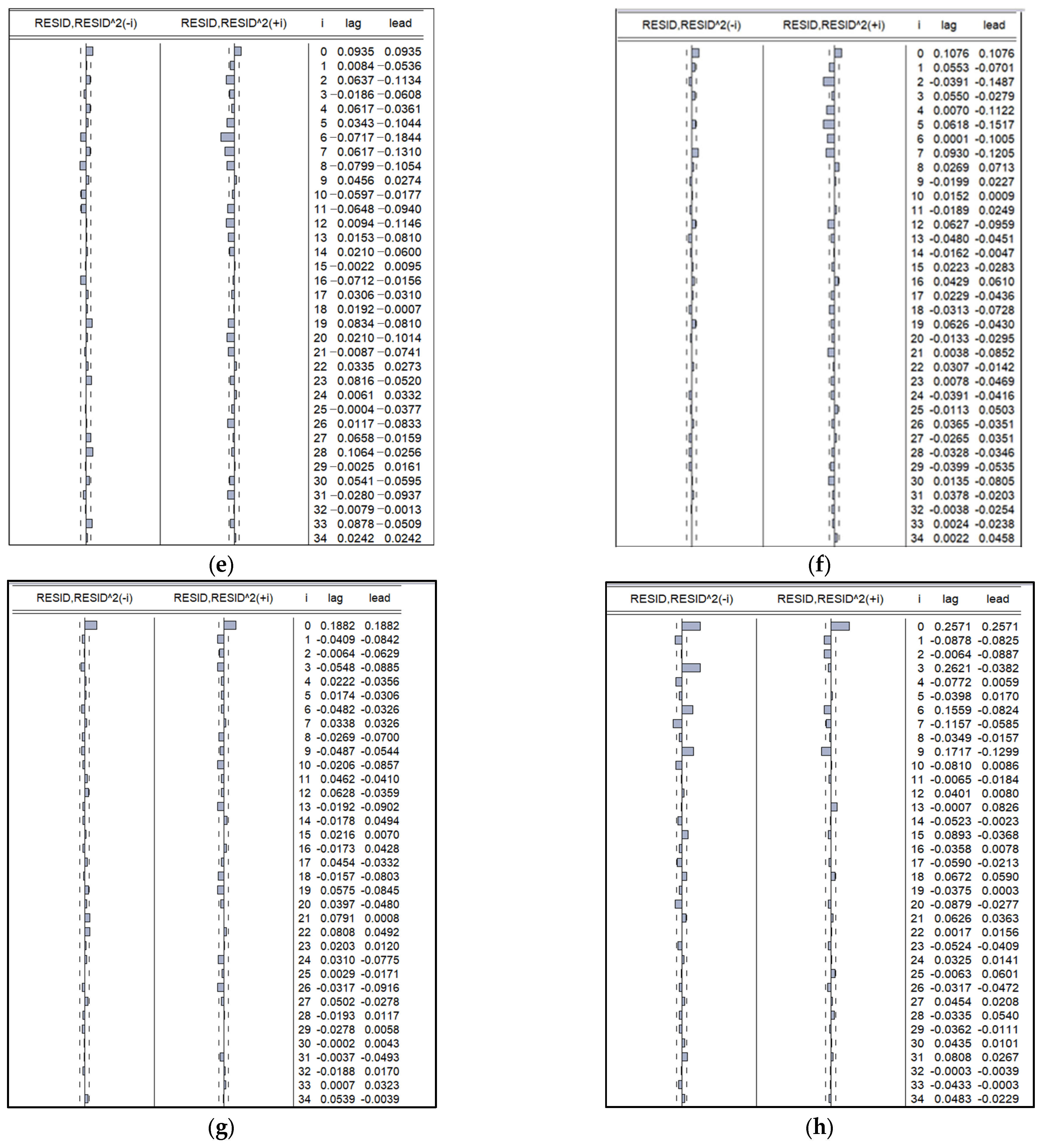
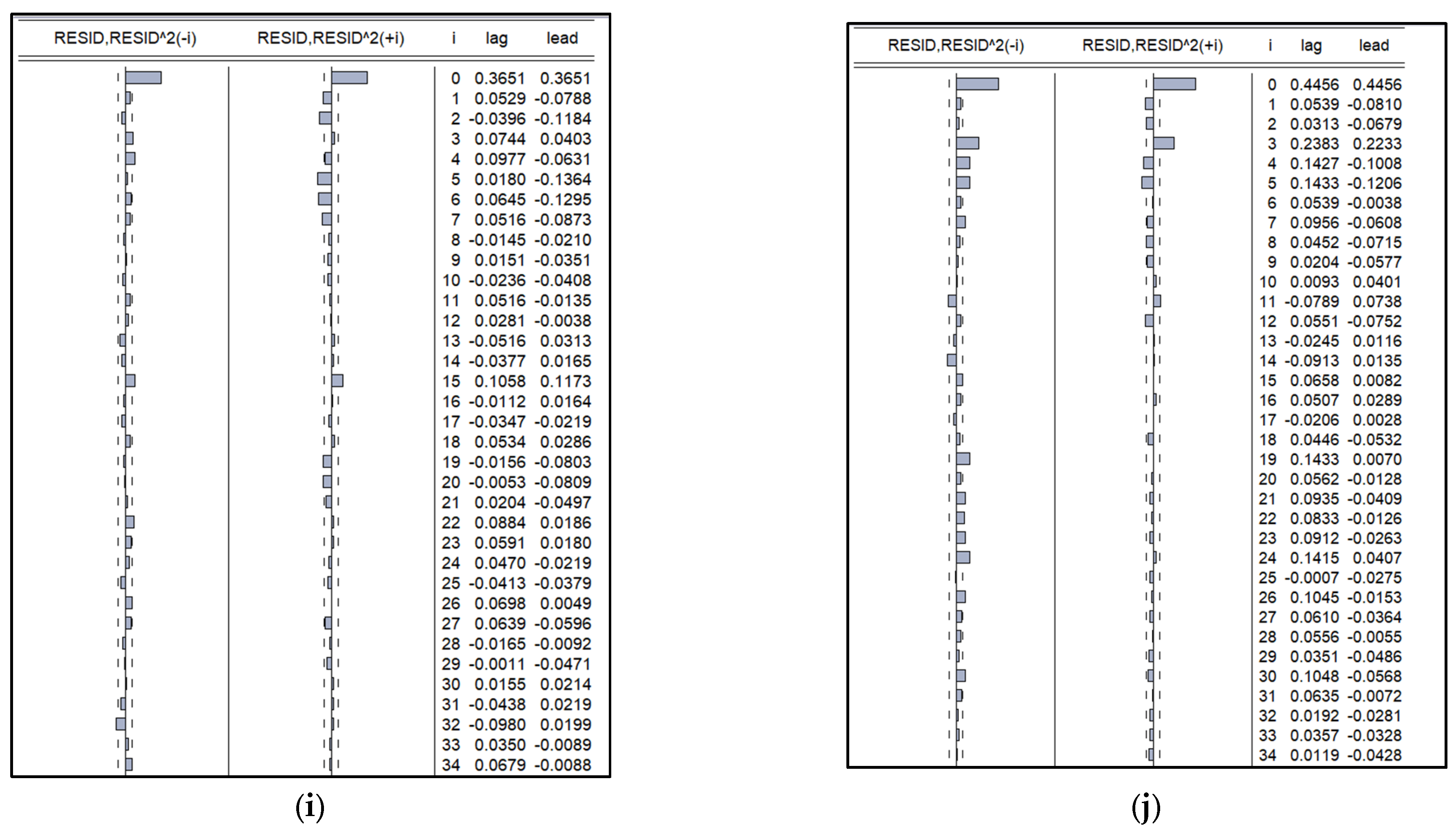
• Check the classic assumptions in the ARMA model, one of which is the assumption of constant and symmetry of random errors. This study’s constant and symmetry checks were carried out using Glejser and cross-correlation (CC) tests, respectively. If the assumptions of constant and symmetry of random errors are met, the experiment continues to stage g, whereas if otherwise, the experiment continues to stage e.
• Identify orders from the GJR-GARCH model. The identification in this study was carried out through the Akaike information criterion (AIC) value. The order with the smallest AIC value is selected.
• Estimate the parameters of the GJR-GARCH model. This assessment in this study was carried out using the maximum likelihood (ML) method. Once this is completed, an ARMA-GJR-GARCH model of each stock data is obtained.
• Diagnostically test errors in the ARMA-GJR-GARCH model.
• Forecast the return of each stock for the next day using each model.
• Resample data by inputting the forecast results of each stock return into the data itself individually.
• Determine the vector of the mean of return $\mathsf{\mu }$ and the covariance matrix $\mathsf{\Sigma }$ from the resampled stock return data.
• Determine the optimal capital weight of each stock using Equation (25).

Visually, the algorithms a to j above are given in Figure 1.

Figure 1. The algorithm for developing stock capital weighting in a portfolio is short and straightforward.

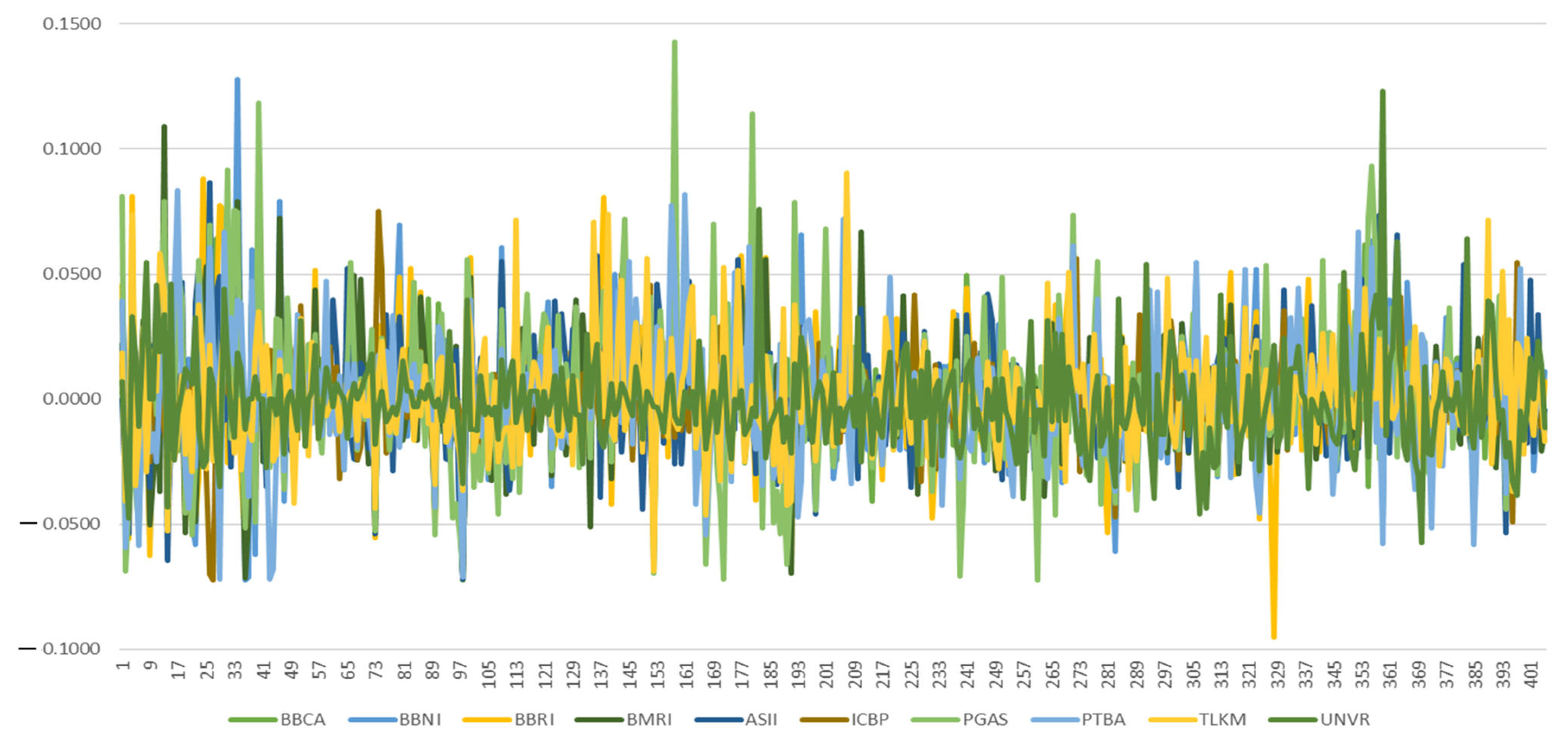
3.2. Data Description

This study used the daily closing price of the top ten stocks traded based on the transaction value on the Indonesia Stock Exchange (IDX), the capital market in Indonesia, until 14 December 2021. The ten stocks are as follows:

• PT. Bank Central Asia Tbk. is coded as BBCA
• PT. Bank Negara Indonesia Tbk. is coded as BBNI.
• PT. Bank Rakyat Indonesia Tbk. is coded as BBRI.
• PT. Bank Mandiri Tbk. is coded as BMRI.
• PT. Astra International Tbk. is coded as ASII.
• PT. Indofood CBP Sukses Makmur Tbk. is coded as ICBP.
• PT. Perusahaan Gas Negara Tbk. is coded as PGAS.
• PT. Bukit Asam Tbk. is coded as PTBA.
• PT. Telekomunikasi Indonesia Tbk. is coded as TLKM.
• PT. Unilever Indonesia Tbk. is coded as UNVR.

The period considered was from 14 April 2020 until 14 December 2021. The data can be openly accessed in the link as follows: https://finance.yahoo.com/ (accessed on 24 March 2022). The graph of each stock return is given in Figure 2. Figure 2 shows that the deviation of daily stock returns at the top and bottom of the zero line appears asymmetrical. The deviation of daily stock returns above the zero line appears to be greater than the deviation of daily stock returns below the zero line. It indicates an asymmetric nature in the deviation of stock returns from the average. Therefore, forecasting stock returns the next day requires a model that can overcome this: the ARMA-GJR-GARCH model.

Figure 2. Visualization of daily returns from the top ten stocks in Indonesia based on transaction values from 14 April 2020 to 14 December 2021.

3.3. Stationarity Test of Data

The stationarity test of each stock return data first uses the Dickey–Fuller Test, as explained in Section 2.3.1. The test was conducted using R Studio software version 4.1.2 via the “tseries” package. With a significance level of 0.05, a summary of the stationarity test results is given in Table 1. Table 1 shows that the test statistical value of each stock return data is less than the critical point. Thus, the conclusion is that $H_0$ from testing on each data is not rejected, which means that all data is stationary, so ARMA modeling can be carried out.

Table 1. Stationarity test results for each stock return datum.

Code		$\mathit{D}{\mathit{F}}_{\mathit{t}\mathit{e}\mathit{s}\mathit{t}}$	${\mathit{t}}_{0.05}$	Conclusion
BBCA		−15.1522	−3.4251	Stock return data are stationary
BBNI		−14.8121
BBRI		−15.2115
BMRI		−16.4812
ASII		−16.0417
ICBP		−15.6242
PGAS		−15.4219
PTBA		−14.8221
TLKM		−18.8046
UNVR		−14.2247

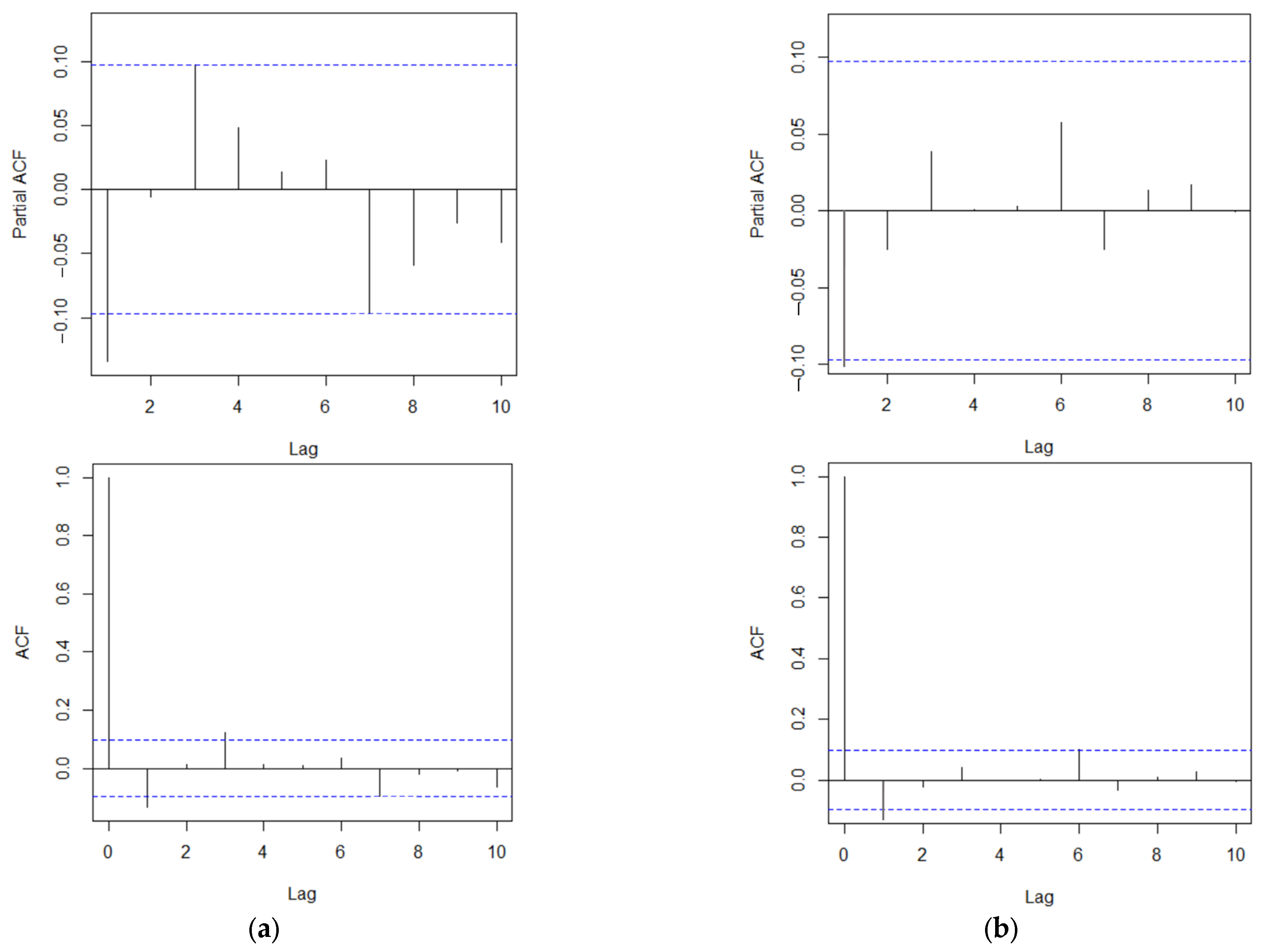
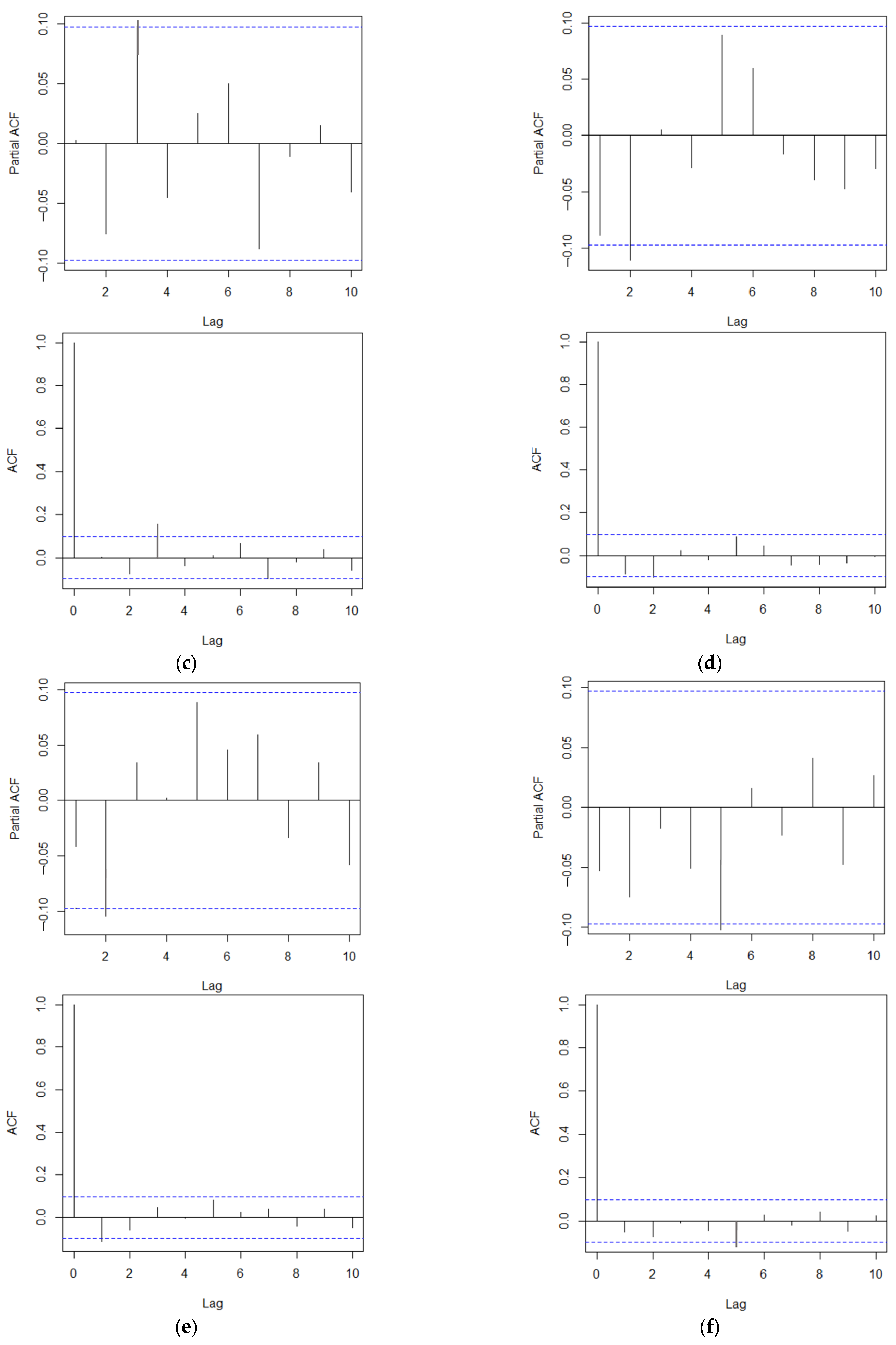
3.4. Order Identification and Parameter Estimation of the ARMA Model

Order identification from the AR and MA models is conducted using partial-autocorrelation function (PACF) and autocorrelation function (ACF) diagrams, respectively. Using the help of EViews 10 software, the PACF and ACF diagrams are given in Figure 3. Figure 3 shows the interpretation of the ARMA model order of each stock. The interpretation of these orders is given in Table 2, using R software version 4.1.2 via the “tseries” package. The estimation results are also given in Table 2.

Figure 3. PACF and ACF from data on the top 10 stocks in Indonesia based on transaction value: BBCA (a), BBNI (b), BBRI (c), BMRI (d), ASII (e), ICBP (f), PGAS (g), ICBP (h), TLKM (i), UNVR (j).

Table 2. The ARMA model of the returns of the top 10 stocks in Indonesia.

No.	Code	ARMA Order	ARMA Model
1.	BBCA	ARMA (1,3)	$r_t=0.0007+0.3482r_{\mathrm{t}-1}-0.4929{\epsilon }_{\mathrm{t}-1}+0.0780{\epsilon }_{t-2}+0.1278{\epsilon }_{t-3}+{\epsilon }_t$
2.	BBNI	ARMA (1,1)	$r_t=0.0013+0.1602r_{\mathrm{t}-1}-0.1990{\epsilon }_{\mathrm{t}-1}+{\epsilon }_t$
3.	BBRI	ARMA (3,3)	$r_t=0.0030-0.5226r_{\mathrm{t}-1}+0.5250r_{t-2}+0.9463r_{t-3}+0.5509{\epsilon }_{\mathrm{t}-1}-0.5726{\epsilon }_{t-2}$$-0.9782{\epsilon }_{t-3}+{\epsilon }_t$
4.	BMRI	ARMA (2,2)	$r_t=0.0012-0.4111r_{\mathrm{t}-1}+0.0260r_{t-2}+0.3152{\epsilon }_{\mathrm{t}-1}-0.1687{\epsilon }_{t-2}+{\epsilon }_t$
5.	ASII	ARMA (2,1)	$r_t=0.0010-1.0793r_{\mathrm{t}-1}-0.1413r_{t-2}+0.9789{\epsilon }_{\mathrm{t}-1}+{\epsilon }_t$
6.	ICBP	ARMA (5,5)	$r_t=-0.0004-0.0847r_{\mathrm{t}-1}-0.0167r_{t-2}-0.2038r_{t-3}-0.5772r_{t-4}+0.4313r_{t-5}$$+0.0449{\epsilon }_{\mathrm{t}-1}-0.0734{\epsilon }_{t-2}+0.1776{\epsilon }_{t-3}+0.5402{\epsilon }_{t-4}-0.5359{\epsilon }_{t-5}+{\epsilon }_t$
7.	PGAS	ARMA (1,2)	$r_t=0.0014-0.7972r_{\mathrm{t}-1}+0.8112{\epsilon }_{\mathrm{t}-1}-0.0865{\epsilon }_{t-2}+{\epsilon }_t$
8.	PTBA	ARMA (1,5)	$r_t=0.0008+0.2626r_{\mathrm{t}-1}-0.2657{\epsilon }_{\mathrm{t}-1}-0.0396{\epsilon }_{t-2}+0.00328{\epsilon }_{t-3}+0.0933{\epsilon }_{t-4}$$-0.0905{\epsilon }_{t-5}+{\epsilon }_t$
9.	TLKM	ARMA (3,3)	$r_t=0.0006+0.0278r_{\mathrm{t}-1}-0.3108r_{t-2}+0.1987r_{t-3}-0.1737{\epsilon }_{\mathrm{t}-1}+0.1402{\epsilon }_{t-2}$$-0.0962{\epsilon }_{t-3}+{\epsilon }_t$
10.	UNVR	ARMA (2,3)	$r_t=-0.0012+1.0761r_{\mathrm{t}-1}-0.5460r_{t-2}-1.0733{\epsilon }_{\mathrm{t}-1}+0.5470{\epsilon }_{t-2}+0.0988{\epsilon }_{t-3}+{\epsilon }_t$

3.5. Checking the Constancy and Symmetry Assumptions of Error Variance in the ARMA Model

Checking the constancy and symmetry of random errors in this study was carried out using the Glejser test and cross-correlation (CC) graphs, as explained in Subsection X.X. The Glejser test was carried out using EViews software version 10. With a significance level of 0.05 and degrees of freedom of 404, a summary of the results of the constant error test is given in Table 3. Table 3 shows that the probability value of each stock return datum is less than 0.05. Thus, the conclusion is that $H_0$ from testing on each datum is not rejected, which means that all data have a random error variance that is not constant. Then, the CC graph of each ARMA model error variance for each stock is given in Figure 4. Figure 4 was obtained using EViews software version 10. Thus, the conclusion is that all data do not have error variance symmetry.

Table 3. Heteroscedasticity test result of the ARMA model’s error variance.

Code	ARMA Model	Probability	Conclusion
BBCA	ARMA (1,3)	0.0004	There is heteroscedasticity in the ARMA model’s error variance.
BBNI	ARMA (1,1)	0.0000
BBRI	ARMA (3,3)	0.0000
BMRI	ARMA (2,2)	0.0000
ASII	ARMA (2,1)	0.0000
ICBP	ARMA (5,5)	0.0000
PGAS	ARMA (1,2)	0.0000
PTBA	ARMA (1,5)	0.0002
TLKM	ARMA (3,3)	0.0000
UNVR	ARMA (2,3)	0.0160

Figure 4. Cross-correlation of ARMA model error variance of the top 10 stocks in Indonesia based on transaction value: BBCA (a), BBNI (b), BBRI (c), BMRI (d), ASII (e), ICBP (f), PGAS (g), ICBP (h), TLKM (i), UNVR (j).

3.6. GJR-GARCH Modeling of Each Stock Return

To overcome the unfulfilled assumptions of constancy and symmetry of the error variance, GJR-GARCH modelling of each error variance in the ARMA model was carried out. The order of each GJR-GARCH model was determined as 1. This was conducted for practical reasons. After the order was determined, the next step was estimating the model’s parameters. This estimation was carried out using the maximum likelihood method. Briefly, using EViews software version 10, the results of determining the order and estimating the parameters of the GJR-GARCH model for each stock are given in Table 4.

Table 4. GJR-GARCH model of the top 10 stocks in Indonesia based on transaction value.

Code	GJR-GARCH (1,1) Model
BBCA	${\sigma }_t^2=8.53\times {10}^{-6}+0.0390{\epsilon }_{t-1}^2+0.1599{\epsilon }_{t-1}^2{\mathrm{I}}_{\mathrm{t}-1}+0.8612{\sigma }_{t-1}^2+{\epsilon }_t$
BBNI	${\sigma }_t^2=7.73\times {10}^{-6}+0.0417{\epsilon }_{t-1}^2+0.0642{\epsilon }_{t-1}^2{\mathrm{I}}_{\mathrm{t}-1}+0.9170{\sigma }_{t-1}^2+{\epsilon }_t$
BBRI	${\sigma }_t^2=9.48\times {10}^{-6}+0.0414{\epsilon }_{t-1}^2+0.1268{\epsilon }_{t-1}^2{\mathrm{I}}_{\mathrm{t}-1}+0.8859{\sigma }_{t-1}^2+{\epsilon }_t$
BMRI	${\sigma }_t^2=2.22\times {10}^{-5}+0.0728{\epsilon }_{t-1}^2+0.1360{\epsilon }_{t-1}^2{\mathrm{I}}_{\mathrm{t}-1}+0.8262{\sigma }_{t-1}^2+{\epsilon }_t$
ASII	${\sigma }_t^2=8.31\times {10}^6++0.0814{\epsilon }_{t-1}^2+0.0657{\epsilon }_{t-1}^2{\mathrm{I}}_{\mathrm{t}-1}+0.9532{\sigma }_{t-1}^2+{\epsilon }_t$
ICBP	${\sigma }_t^2=7.12\times {10}^{-5}+0.0785{\epsilon }_{t-1}^2+0.1898{\epsilon }_{t-1}^2{\mathrm{I}}_{\mathrm{t}-1}+0.5813{\sigma }_{t-1}^2+{\epsilon }_t$
PGAS	${\sigma }_t^2=4.31\times {10}^{-5}+0.0631{\epsilon }_{t-1}^2+0.0634{\epsilon }_{t-1}^2{\mathrm{I}}_{\mathrm{t}-1}+0.8645{\sigma }_{t-1}^2+{\epsilon }_t$
PTBA	${\sigma }_t^2=3.31\times {10}^{-5}+0.0727{\epsilon }_{t-1}^2+0.0566{\epsilon }_{t-1}^2{\mathrm{I}}_{\mathrm{t}-1}+0.8527{\sigma }_{t-1}^2+{\epsilon }_t$
TLKM	${\sigma }_t^2=9.84\times {10}^{-6}+0.0363{\epsilon }_{t-1}^2+0.0701{\epsilon }_{t-1}^2{\mathrm{I}}_{\mathrm{t}-1}+0.9095{\sigma }_{t-1}^2+{\epsilon }_t$
UNVR	${\sigma }_t^2=1.05\times {10}^{-5}+0.0923{\epsilon }_{t-1}^2+0.1512{\epsilon }_{t-1}^2{\mathrm{I}}_{\mathrm{t}-1}+0.7072{\sigma }_{t-1}^2+{\epsilon }_t$

3.7. Error Diagnostic Test and Accuracy Check of ARMA-GJR-GARCH Model

Error diagnostic tests included tests for normality and independence of error from the ARMA-GJR-GARCH model. The normality test was conducted using the Kolmogorov–Smirnov test with a significance level of 0.05. In contrast, the error independence test used the Ljung–Box test with a significance level of 0.05. The results of both can be seen in Section 2.3.3 and Section 2.3.4. A summary of the tests for normality and independence of error are given in Table 5 and Table 6, respectively. Table 5 and Table 6 show that the $H_0$ from both tests is rejected. It shows that the error meets the assumptions of normality and independence.

Table 5. Error normality test results for each ARMA-GJR-GARCH model.

Code	${\mathit{K}\mathit{S}}_{\mathit{t}\mathit{e}\mathit{s}\mathit{t}}$	${\mathit{K}\mathit{S}}_{0.05}$	Conclusion
BBCA	0.0564	0.0675	The error of each ARMA-GJR-GARCH model is normally distributed
BBNI	0.0653
BBRI	0.0429
BMRI	0.0461
ASII	0.0593
ICBP	0.0663
PGAS	0.0641
PTBA	0.0673
TLKM	0.0419
UNVR	0.0578

Table 6. Error independence test results for each ARMA-GJR-GARCH model.

Code	${\mathit{L}\mathit{B}}_{\mathit{t}\mathit{e}\mathit{s}\mathit{t}}$	${\mathit{L}\mathit{B}}_{0.05}$	Conclusion
BBCA	45.3311	46.1943	The error of each ARMA-GJR-GARCH model is independent of the others
BBNI	45.1821	48.6024
BBRI	43.1391	43.7730
BMRI	36.2593	46.1943
ASII	43.3852	47.3999
ICBP	31.3604	38.8851
PGAS	46.9329	47.3999
PTBA	38.8132	43.7730
TLKM	39.9226	43.7730
UNVR	44.9590	44.9853

Next, the checking of the accuracy of the ARMA-GJR-GARCH model for each stock needs to be carried out. This examination used the mean absolute error (MAE) and root-mean-squared error (RMSE) measures. The MAE and RMSE of each AR-MA-GJR-GARCH model for each stock are given in Table 7. Table 7 shows that the MAE and RMSE of each model look small. It indicates that the model is accurate and suitable for use.

Table 7. MAE and RMSE values.

Code	MAE	RMSE
BBCA	0.0139	0.0209
BBNI	0.0169	0.0245
BBRI	0.0158	0.0237
BMRI	0.0234	0.0327
ASII	0.0163	0.0229
ICBP	0.0116	0.0177
PGAS	0.0219	0.0312
PTBA	0.0184	0.0274
TLKM	0.0144	0.0203
UNVR	0.0136	0.0207

3.8. Forecasting Mean of Return One Day Ahead

After the ARMA-GJR-GARCH model for each stock was obtained, the mean of return one day ahead was predicted. This forecast was then used as a new sample for the next day in the mean-VaR model. The forecast results of the mean of return for each stock are given in Table 8. Table 8 also provides a forecast of the error variance.

Table 8. Forecasting of means and variances of stock returns.

Code	$\mathbf{Forecast}\mathbf{of}\mathbf{Mean}\mathbf{of}\mathbf{Return}({\widehat{\mathit{\mu }}}_{\mathit{t}}$)	$\mathbf{Forecast}\mathbf{of}\mathbf{Variance}\mathbf{of}\mathbf{Error}({\widehat{\mathit{\sigma }}}_{\mathit{t}}^2$)
BBCA	0.00661	0.00107
BBNI	0.00026	0.00523
BBRI	0.00030	0.00382
BMRI	0.00205	0.04064
ASII	0.00026	0.05490
ICBP	−0.00133	0.01291
PGAS	0.00081	0.02410
PTBA	−0.00129	0.08080
TLKM	0.00326	0.01180
UNVR	0.00227	0.07700

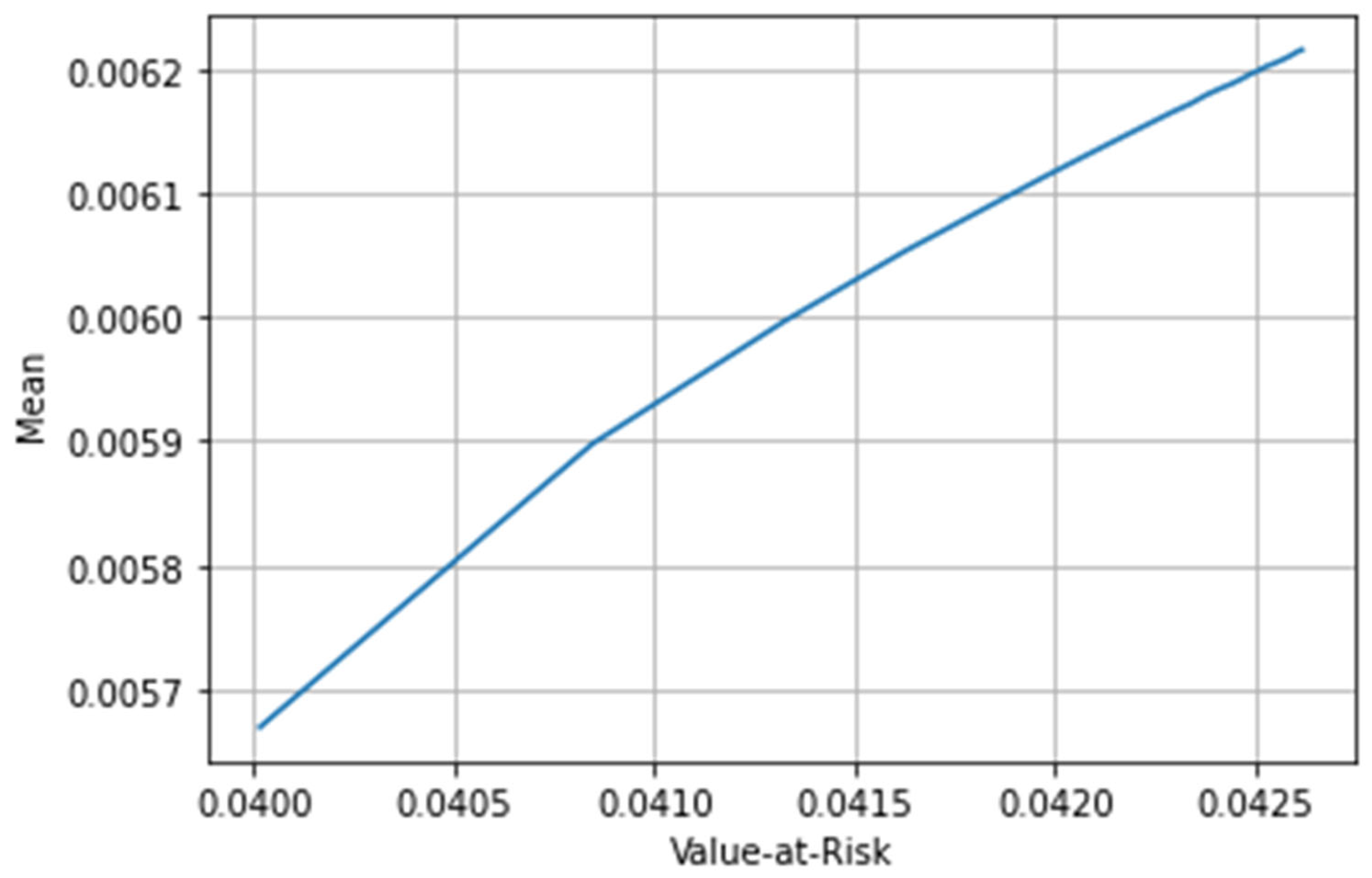
3.9. Portfolio Optimization Process

The process of optimizing the portfolio using mean-VaR first looks for covariance matrices between stocks. The calculation is assisted by using Excel 2016 software and produces values as follows:

$$\mathsf{\Sigma }=\left[\begin{array}{cccccccccc}0.00107& 0.00024& 0.00023& 0.00025& 0.00020& 0.00011& 0.00021& 0.00019& 0.00017& 0.00014\\ 0.00024& 0.00052& 0.00042& 0.00045& 0.00033& 0.00017& 0.00042& 0.00026& 0.00023& 0.00016\\ 0.00023& 0.00042& 0.00038& 0.00040& 0.00028& 0.00016& 0.00035& 0.00023& 0.00022& 0.00015\\ 0.00025& 0.00045& 0.00040& 0.00406& 0.00032& 0.00016& 0.00037& 0.00025& 0.00021& 0.00016\\ 0.00020& 0.00033& 0.00028& 0.00032& 0.00055& 0.00015& 0.00032& 0.00021& 0.00021& 0.00017\\ 0.00011& 0.00017& 0.00016& 0.00016& 0.00015& 0.00129& 0.00018& 0.00015& 0.00013& 0.00017\\ 0.00021& 0.00042& 0.00035& 0.00037& 0.00032& 0.00018& 0.00024& 0.00035& 0.00026& 0.00019\\ 0.00019& 0.00026& 0.00023& 0.00025& 0.00021& 0.00015& 0.00035& 0.00081& 0.00022& 0.00019\\ 0.00017& 0.00023& 0.00022& 0.00021& 0.00021& 0.00013& 0.00026& 0.00022& 0.00012& 0.00015\\ 0.00014& 0.00016& 0.00015& 0.00016& 0.00017& 0.00017& 0.00019& 0.00019& 0.00015& 0.00008\end{array}\right]$$

After obtaining the covariance matrix $\mathsf{\Sigma }$, then the next step is the calculation of the inverse covariance matrix. The result of this calculation is shown as follows:

$${\mathsf{\Sigma }}^{-1}=\left[\begin{array}{cccccccccc}958.7062& -38.1084& -51.7294& -4.6986& -2.8700& -7.0017& -6.6010& -1.9216& -11.8235& -1.4302\\ -38.1084& 195.0594& -18.2740& -1.6778& -0.8984& -1.9383& -2.7217& -0.4497& -2.7620& -0.2711\\ -51.7294& -18.2740& 267.8453& -2.0448& -1.0313& -2.4412& -2.9624& -0.5511& -3.6729& -0.3711\\ -4.6986& -1.6778& -2.0448& 24.6792& -0.1008& -0.2010& -0.2686& -0.0519& -0.2909& -0.0323\\ -2.8700& -0.8984& -1.0313& -0.1008& 18.2394& -0.1549& -0.1828& -0.0328& -0.2395& -0.0295\\ -7.0017& -1.9383& -2.4412& -0.2010& -0.1549& 77.5971& -0.4392& -0.1060& -0.6572& -0.1428\\ -6.6010& -2.7217& -2.9624& -0.2686& -0.1828& -0.4392& 41.6611& -0.1435& -0.6889& -0.0746\\ -1.9216& -0.4497& -0.5511& -0.0519& -0.0328& -0.1060& -0.1435& 12.3855& -0.1796& -0.0246\\ -11.8235& -2.7620& -3.6729& -0.2909& -0.2395& -0.6572& -0.6889& -0.1796& 85.0759& -0.1301\\ -1.4302& -0.2711& -0.3711& -0.0323& -0.0295& -0.1428& -0.0746& -0.0246& -0.1301& 12.9917\end{array}\right]$$

Then, the next is the determination of the average transpose vector value ${\mathsf{\mu }}^T$, expressed as follows:

$${\mathsf{\mu }}^T=\left[\begin{array}{cccccccccc}0.0007& 0.0013& 0.0010& 0.0012& 0.0010& -0.0004& 0.0014& 0.0007& 0.0006& -0.0012\end{array}\right]$$

Then, the one vector is expressed as follows:

$${\mathbf{e}}^T=\left[\begin{array}{cccccccccc}1& 1& 1& 1& 1& 1& 1& 1& 1& 1\end{array}\right].$$

Covariance matrix or ${\mathsf{\Sigma }}^{-1}$ were used to calculate the composition of the efficient portfolio weight in the model used using Excel 2016 software. Refer to Equation (25), by using vector ${\mathsf{\mu }}^T$, ${\mathbf{e}}^T$ and matrix ${\mathsf{\Sigma }}^{-1}$ the weight vector value can be calculated $\mathbf{w}$. Parameter $\tau$ is called risk tolerance and simulated with several values that meet ${\mathbf{e}}^T\mathbf{w}=1.$ In addition, a risk tolerance must produce a nonnegative value of $\mathbf{w}$.

3.10. Discussion

This section describes the determination of the optimum weight. In addition, this section also analyzes the relationship between value-at-risk to ratio, risk tolerance to average, and risk tolerance to value-at-risk. Optimum weight is divided into two, namely the minimum and maximum weight. The minimum weight is the weight used to produce the smallest mean value, while the maximum weight is the weight that produces the largest mean value. Determination of the optimum weight is carried out in several steps. The first step is to determine the percentile value of VaR. In this study, we used 0.01 as significant level, and the selected percentile value is $z_{0.01}=-2.33$ used to determine $\lambda$. Second is the determination of the interval of risk tolerance $\tau$. This stage is carried out using the trial-and-error method so that all asset weights are positive. Briefly, we derived the risk tolerance interval $0\le \tau <16.56$ with an increase of 0.72. A risk tolerance greater than 17.28 or $\tau \ge 17.28$ is said not to be feasible because it produces a negative weight. Finally, the minimum weight from Appendix A is obtained when the risk tolerance is 0 with a return of 0.005670, while the maximum weight is obtained at a risk tolerance of 16.56 with a return of 0.006214. The complete results of the trials and errors can be seen in Appendix A.

Then, we analyzed the value-at-risk relationship to the ratio. This relationship can be explained as the higher the value-at-risk, the higher the ratio obtained. This is presented in Figure 5.

Figure 5. Value-at-risk relationship to ratio.

Next, we carried out the analysis of the mean of return relationship to the ratio. This relationship can be explained as the higher the mean of return, the higher the ratio obtained. This is presented in Figure 6.

Figure 6. Mean of return relationship to ratio.

We then proceeded to analyze the relationship between risk tolerance and value-at-risk. Based on the analysis that has been done, the greater the risk tolerance, the higher the value-at-risk. For more details, see Figure 7.

Figure 7. Relationship between risk tolerance and value-at-risk.

Next, we analyzed the relationship between risk tolerance and average. Based on the analysis obtained, it was found that the greater the risk tolerance, the higher the average. Vice versa, the greater the average, the higher the risk tolerance. For more details, see Figure 8.

Figure 8. Relationship between risk tolerance and mean of return.

Then, the value-at-risk analysis was carried out on average. Based on the analysis that had been carried out, it was known that the greater the average return value, the greater the value-at-risk obtained. These results can be seen clearly in Figure 9.

Figure 9. Relationship between value-at-risk to mean of return.

Next, we analyzed the comparison of the optimal mean of return obtained through the ARMA-GJR-GARCH mean-VaR mechanism and the mean-variance model. The mean-variance model is expressed as follows:

$$\begin{gathered} \mathrm{m}\mathrm{a}\mathrm{x}.\tau {\mathbf{w}}^T\mathsf{\mu }-{\mathbf{w}}^T\mathsf{\Sigma }\mathbf{w} \\ \mathrm{s}.\mathrm{t}.{\mathbf{e}}^T\mathbf{w}=1. \end{gathered}$$

(32)

The solution is as follows:

$$\mathbf{w}={\mathsf{\Sigma }}^{-1}\left(\tau \mathsf{\mu }+\lambda \mathbf{e}\right),$$

(33)

where

$$\lambda =\frac{1-\tau {\mathbf{e}}^T{\mathsf{\Sigma }}^{-1}\mathsf{\mu }}{{\mathbf{e}}^T{\mathsf{\Sigma }}^{-1}\mathbf{e}}.$$

(34)

A comparison of the optimal mean of return from the mechanism in this study and the model in Equation (32) is given in Table 9.

Table 9. A comparison of the optimal mean of return from the mechanism in this study and the mean-variance model.

Model	Mean of Return
ARMA-GJR-GARCH mean-VaR	0.006214
Mean variance	0.005514

Table 9 shows that the mean of return obtained from the mechanism in this study provides a greater value than the mean-variance model. Therefore, the mechanism in this study can be used convincingly.

4. Conclusions

This study examines the application of the mean-VaR optimization model to determine the weight of share capital allocation in investment portfolios. The stocks used are stocks that have asymmetric return volatility and are listed on the Indonesia Stock Exchange. The ARMA-GJR-GARCH time series model accommodates the asymmetric shape of these stocks.

The prediction results from the time series model were used as the estimated return of each stock the next day. These estimates were then used as the average return vector $\mathsf{\mu }$ in the mean-VaR model. The results of capital weighting were 84% BBCA, 2.5% BBNI, 5.5% BBRI, 0.01% BMRI, 0.03% ASII, 0.06% ICBP, 0.3% PTBA, 0.0% PGAS, 0.2% TLKM, and 0.02% UNVR. Then, if value-at-risk increased, the ratio and average also increased. If risk tolerance increased, then value-at-risk and average increasd. Based on this research, the most efficient portfolio with the highest value of return and value-at-risk is 0.006214 and 0.042608.

References

- Black, F.; Litterman, R. Global Portfolio Optimization. Financ. Anal. J. 1992, 48, 28–43. [Google Scholar] [CrossRef]
- Bollerslev, T. Generalized Autoregressive Conditional Heteroskedasticity. J. Econom. 1986, 31, 307–327. [Google Scholar] [CrossRef]
- Charles, A.; Darné, O. The Accuracy of Asymmetric GARCH Model Estimation. Int. Econ. 2019, 157, 179–202. [Google Scholar] [CrossRef]
- Xiong, J.; Zhou, X.Y. Mean-Variance Portfolio Selection under Partial Information. SIAM J. Control Optim. 2007, 46, 156–175. [Google Scholar] [CrossRef]
- Su, Y.C.; Huang, H.C.; Lin, Y.J. GJR-GARCH Model in Value-at-Risk of Financial Holdings. Appl. Financ. Econ. 2011, 21, 1819–1829. [Google Scholar] [CrossRef]
- Kalayci, C.B.; Ertenlice, O.; Akbay, M.A. A Comprehensive Review of Deterministic Models and Applications for Mean-Variance Portfolio Optimization. Expert Syst. Appl. 2019, 125, 345–368. [Google Scholar] [CrossRef]
- Al Janabi, M.A.M. Multivariate Portfolio Optimization under Illiquid Market Prospects: A Review of Theoretical Algorithms and Practical Techniques for Liquidity Risk Management. J. Model. Manag. 2021, 16, 288–309. [Google Scholar] [CrossRef]
- Nur Aini, N.S.; Lutfi, L. The Influence of Risk Perception, Risk Tolerance, Overconfidence, and Loss Aversion towards Investment Decision Making. J. Econ. Bus. Account. Ventur. 2019, 21, 401. [Google Scholar] [CrossRef]
- Pak, O.; Mahmood, M. Impact of Personality on Risk Tolerance and Investment Decisions. Int. J. Commer. Manag. 2015, 25, 370–384. [Google Scholar] [CrossRef]
- Hyndman, R.J.; Khandakar, Y. Automatic Time Series Forecasting: The Forecast Package for R. J. Stat. Softw. 2008, 27, 1–22. [Google Scholar] [CrossRef]
- Fu, R.; Zhang, Z.; Li, L. Using LSTM and GRU Neural Network Methods for Traffic Flow Prediction. In Proceedings of the 2016 31st Youth Academic Annual Conference of Chinese Association of Automation (YAC), Wuhan, China, 1–13 November 2016; pp. 324–328. [Google Scholar]
- Sukono, S.; Parmikanti, K.; Lisnawati, L.; Gw, S.H.; Saputra, J. Mean-Var Investment Portfolio Optimization Under Capital Asset Pricing Model (CAPM) with Nerlove Transformation: An Empirical Study Using Time Series Approach. Ind. Eng. Manag. Syst. 2020, 19, 498–509. [Google Scholar] [CrossRef]
- Suganthi, L.; Samuel, A.A. Energy Models for Demand Forecasting—A Review. Renew. Sustain. Energy Rev. 2012, 16, 1223–1240. [Google Scholar] [CrossRef]
- Valipour, M.; Banihabib, M.E.; Behbahani, S.M.R. Comparison of the ARMA, ARIMA, and the Autoregressive Artificial Neural Network Models in Forecasting the Monthly Inflow of Dez Dam Reservoir. J. Hydrol. 2013, 476, 433–441. [Google Scholar] [CrossRef]
- Vaibhava Lakshmi, R.; Radha, S. Time Series Forecasting for the Adobe Software Company’s Stock Prices Using ARIMA (BOX-JENKIN’) Model. J. Phys. Conf. Ser. 2021, 2115, 012044. [Google Scholar] [CrossRef]
- Hidayana, R.A.; Napitupulu, H.; Sukono, S. An Investment Decision-Making Model to Predict the Risk and Return in Stock Market: An Application of ARIMA-GJR-GARCH. Decis. Sci. Lett. 2022, 11, 235–246. [Google Scholar] [CrossRef]
- Dritsaki, C. An Empirical Evaluation in GARCH Volatility Modeling: Evidence from the Stockholm Stock Exchange. J. Math. Financ. 2017, 07, 366–390. [Google Scholar] [CrossRef]
- Zhang, L.; Zoli, E. Leaning against the Wind: Macroprudential Policy in Asia. J. Asian Econ. 2016, 42, 33–52. [Google Scholar] [CrossRef]
- Yin, R.; Newman, D.H.; Siry, J. Testing for Market Integration among Southern Pine Regions. J. For. Econ. 2002, 8, 151–166. [Google Scholar] [CrossRef]
- Ma, Z.-G.; Ma, C.-Q. Pricing Catastrophe Risk Bonds: A Mixed Approximation Method. Insur. Math. Econ. 2013, 52, 243–254. [Google Scholar] [CrossRef]
- Ghasemi, A.; Zahediasl, S. Normality Tests for Statistical Analysis: A Guide for Non-Statisticians. Int. J. Endocrinol. Metab. 2012, 10, 486–489. [Google Scholar] [CrossRef]
- Liu, Q.; Liu, X.; Jiang, B.; Yang, W. Forecasting Incidence of Hemorrhagic Fever with Renal Syndrome in China Using ARIMA Model. BMC Infect. Dis. 2011, 11, 218. [Google Scholar] [CrossRef] [PubMed]
- Sukono; Juahir, H.; Ibrahim, R.A.; Saputra, M.P.A.; Hidayat, Y.; Prihanto, I.G. Application of Compound Poisson Process in Pricing Catastrophe Bonds: A Systematic Literature Review. Mathematics 2022, 10, 2668. [Google Scholar] [CrossRef]
- Tadesse, K.B.; Dinka, M.O. Application of SARIMA Model to Forecasting Monthly Flows in Waterval River, South Africa. J. Water Land Dev. 2017, 35, 229–236. [Google Scholar] [CrossRef]
- Mohajerin Esfahani, P.; Kuhn, D. Data-Driven Distributionally Robust Optimization Using the Wasserstein Metric: Performance Guarantees and Tractable Reformulations. Math. Program. 2018, 171, 115–166. [Google Scholar] [CrossRef]
- Kolm, P.N.; Tütüncü, R.; Fabozzi, F.J. 60 Years of Portfolio Optimization: Practical Challenges and Current Trends. Eur. J. Oper. Res. 2014, 234, 356–371. [Google Scholar] [CrossRef]
- Xidonas, P.; Steuer, R.; Hassapis, C. Robust Portfolio Optimization: A Categorized Bibliographic Review. Ann. Oper. Res. 2020, 292, 533–552. [Google Scholar] [CrossRef]
- Guo, Y.; Zhou, W.; Luo, C.; Liu, C.; Xiong, H. Instance-Based Credit Risk Assessment for Investment Decisions in P2P Lending. Eur. J. Oper. Res. 2016, 249, 417–426. [Google Scholar] [CrossRef]
- Ponsich, A.; Jaimes, A.L.; Coello, C.A.C. A Survey on Multiobjective Evolutionary Algorithms for the Solution of the Portfolio Optimization Problem and Other Finance and Economics Applications. IEEE Trans. Evol. Comput. 2013, 17, 321–344. [Google Scholar] [CrossRef]
- Kon, S.J. Models of Stock Returns—A Comparison. J. Financ. 1984, 39, 147. [Google Scholar] [CrossRef]
- Prakash, A.J.; Chang, C.-H.; Pactwa, T.E. Selecting a Portfolio with Skewness: Recent Evidence from US, European, and Latin American Equity Markets. SSRN Electron. J. 2003, 27, 1375–1390. [Google Scholar] [CrossRef]
- Rockafellar, R.T.; Uryasev, S. Optimization of Conditional Value-at-Risk. J. Risk 2000, 2, 21–41. [Google Scholar] [CrossRef]
- Rockafellar, R.T.; Uryasev, S. Conditional Value-at-Risk for General Loss Distributions. J. Bank. Financ. 2002, 26, 1443–1471. [Google Scholar] [CrossRef]
- Gaivoronski, A.; Pflug, G. Value-at-Risk in Portfolio Optimization: Properties and Computational Approach. J. Risk 2005, 7, 1–31. [Google Scholar] [CrossRef]
- Pérignon, C.; Smith, D.R. The Level and Quality of Value-at-Risk Disclosure by Commercial Banks. J. Bank. Financ. 2010, 34, 362–377. [Google Scholar] [CrossRef]
- Purwandari, T.; Riaman; Hidayat, Y.; Sukono; Ibrahim, R.A.; Hidayana, R.A. Selecting and Weighting Mechanisms in Stock Portfolio Design Based on Clustering Algorithm and Price Movement Analysis. Mathematics 2023, 11, 4151. [Google Scholar] [CrossRef]
- Lwin, K.T.; Qu, R.; MacCarthy, B.L. Mean-VaR Portfolio Optimization: A Nonparametric Approach. Eur. J. Oper. Res. 2017, 260, 751–766. [Google Scholar] [CrossRef]
- Sukono; Sidi, P.; bin Bon, A.T.; Supian, S. Modeling of Mean-VaR Portfolio Optimization by Risk Tolerance When the Utility Function Is Quadratic. In Proceedings of the 2016 2nd International Conference on Applied Statistics (ICAS II), West Java, Indonesia, 27–28 September 2016; p. 020035. [Google Scholar]
- Lin, X.; Floudas, C.A.; Kallrath, J. Global Solution Approach for a Nonconvex MINLP Problem in Product Portfolio Optimization. J. Glob. Optim. 2005, 32, 417–431. [Google Scholar] [CrossRef]
- Cesarone, F.; Scozzari, A.; Tardella, F. An Optimization–Diversification Approach to Portfolio Selection. J. Glob. Optim. 2020, 76, 245–265. [Google Scholar] [CrossRef]
Disclaimer/Publisher’s Note: The statements, opinions and data contained in all publications are solely those of the individual author(s) and contributor(s) and not of MDPI and/or the editor(s). MDPI and/or the editor(s) disclaim responsibility for any injury to people or property resulting from any ideas, methods, instructions or products referred to in the content. |
© 2023 by the authors. Licensee MDPI, Basel, Switzerland. This article is an open access article distributed under the terms and conditions of the Creative Commons Attribution (CC BY) license (https://creativecommons.org/licenses/by/4.0/).