An Algorithm That Adjusts the Stepsize to Be Self-Adaptive with an Inertial Term Aimed for Solving Split Variational Inclusion and Common Fixed Point Problems

Abstract

In this research paper, we present a new inertial method with a self-adaptive technique for solving the split variational inclusion and fixed point problems in real Hilbert spaces. The algorithm is designed to choose the optimal choice of the inertial term at every iteration, and the stepsize is defined self-adaptively without a prior estimate of the Lipschitz constant. A convergence theorem is demonstrated to be strong even under lenient conditions and to showcase the suggested method’s efficiency and precision. Some numerical tests are given. Moreover, the significance of the proposed method is demonstrated through its application to an image reconstruction issue.

1. Introduction

In this paper, we consider the Split Variational Inclusion Problem (SVIP) introduced by Moudafi [1], which is the problem of finding the null point of a monotone operator in a Hilbert space whose image under a bounded linear operator belongs to another Hilbert space. Mathematically, the problem is defined as follows: find

$$a^{*}\in H_1\mathrm{such}\mathrm{that}0\in m_1\left(a^{*}\right)$$

(1)

and

$$b^{*}=B{a}^{*}\mathrm{solves}0\in m_2\left(b^{*}\right),$$

(2)

where 0 is called the zero vector, with $H_1$ and $H_2$ being both real Hilbert spaces together with the multivalued maximal monotone mappings, $m_i:H_i\to 2^{H_i}$ where $i=1,2$. Furthermore, the bounded linear operator is denoted by $B:H_1\to H_2$. We denote the solution set of (1) and (2) by $\mathrm{\Gamma }$.

An operator $m:H\to 2^H$ is called:

(i)

Monotone if

$$⟨k-x,a-b⟩\ge 0\forall k\in m\left(a\right),x\in m\left(b\right)\forall a,b\in H.$$

(ii)

Maximal monotone if the graph of any monotone mapping does not properly contain graph $G\left(m\right)$ of m, where:

$$G\left(m\right)=\{(a,k)\in H_1\times H_1|k\in m\left(a\right)\}.$$

(iii)

The symbol used to represent the solution of m when a certain value $\lambda$ greater than zero is used as a parameter is called the resolvent, which is denoted by $J_{\lambda }^m$:

$$J_{\lambda }^m\left(a\right)={(I+\lambda m)}^{-1}\left(a\right)\forall a\in H.$$

Other nonlinear optimization problems, such as split feasibility problems, split minimization problems, split variational inequality, split zero problems, and split equilibrium problems, can all be generalized by the SVIP; see [2,3,4]. Reducing SVIPs to split feasibility problems is important when modeling the intensity-modulating radiation therapy (IMRT) treatment planning. Moreso, the SVIPs play important roles in formulating many problems arising from engineering, economics, medicine, data compression, and sensor networks [5,6].

Recently, several authors have introduced some iterative methods for solving SVIPs, which have improved over time. In 2002, Byrne et al. [7] first introduced a weak convergence method for solving SVIPs as follows:

$$a_{n+1}=J_{\lambda }^{m_1}(a_n+\gamma B^{*}(J_{\lambda }^{m_2}-I)B{a}_n),$$

(3)

for some parameter $\lambda >0$, we have $B^{*}$ representing the adjoint of B together with $L=\left|\right|B^{*}B\left|\right|$, $\gamma \in (0,\frac{2}{L})$ and $J_{\lambda }^{m_i}={(I+\lambda m_i)}^{-1}$ known as the resolvent operator for $m_i$ (with $i=1,2$). The sequence $\left\{a_n\right\}$ generated by $\left(3\right)$ was proved to converge weakly to $a^{*}$ under some certain conditions. Moudafi [1] proposed an iterative method that helps to solve SVIP with inverse strongly monotone operators; he also obtained weak convergence results using the following iteration:

$$a_{n+1}=U(a_n+\gamma B^{*}(F-I)B{a}_n)\forall n\in N,$$

(4)

where $\lambda >0,\gamma \in (0,\frac{2}{L})$ with L being the largest absolute value of the operator $B^{*}B$, $U=J_{\lambda }^{m_1}(I-\lambda \varphi )$ and $F=J_{\lambda }^{m_2}(I-\lambda \phi )$, and $J_{\lambda }^{m_1}$ together with $J_{\lambda }^{m_2}$ are the resolvent operators of $m_1$ and $m_2$, respectively. Lastly, let $\varphi :H_1\to H_1$ and $\phi :H_2\to H_2$ be single-valued operators. Marino and Xu [8] presented an iterative scheme that considers the strong convergence of the viscosity approximation method introduced by Moudafi [9]:

$$a_{n+1}=(I-{\alpha }_{n}G)F{a}_n+{\alpha }_{n}G\beta f\left(a_n\right)n\ge 0,$$

(5)

f is a function that contracts on the set H with the contraction coefficient $\alpha \in (0,1)$. G is a linear operator that is strongly positive and bounded on H with a constant $\mu$. The parameter is defined in a way that $0<\beta <\frac{\mu }{\alpha }$, exclusive. There exists a nonexpansive mapping F and a sequence $\left\{{\alpha }_n\right\}$ that takes values in $(0,1)$. The strong convergence of the sequence $\left\{a_n\right\}$ obtained from (5) to the fixed point $a^{*}\in Fix\left(F\right):=\{a^{*}:F\left(a^{*}\right)=a^{*}\}$ has been proven. Furthermore, $a^{*}$ serves as the unique solution of the variational inequality:

$$⟨(G-\beta f)a^{*},a-a^{*}⟩\ge 0,a\in C.$$

(6)

The presentation of the optimality condition for the minimization problem is included as follows:

$$\underset{a\in C}{min}\frac{1}{2}⟨Ga,a⟩-h\left(a\right),$$

the function h is a potential function for $\beta f$, i.e.,

$$h\left(a\right)=\left\{\beta f\right(a)fora\in H\}.$$

In 2014, Kazmi and Rizvi [10] were inspired by the work of Byrne et al. (3) to propose the following iteration for solving SVIPs. For a given $a_1\in H_1$,

$$\left\{\begin{array}{c}{k}_n=J_{\lambda }^{m_1}(a_n+\gamma B^{*}(J_{\lambda }^{m_2}-I)B{a}_n),\hfill \\ a_{n+1}={\alpha }_{n}f\left(a_n\right)+(1-{\alpha }_n)S{k}_{n}n\ge 1,\hfill \end{array}\right.$$

(7)

where $\alpha >0,\gamma \in (0,\frac{1}{L})$, L is the spectral radius of the operator $B^{*}B$ and sequence $\left\{{\alpha }_n\right\}$ satisfies the conditions: ${lim}_{n\to \infty }{\alpha }_n=0$, ${\sum }_{n=0}^{\infty }{\alpha }_n=\infty$, and ${\sum }_{n=0}^{\infty }|{\alpha }_n-{\alpha }_{n-1}|<\infty$. The sequences $\left\{k_n\right\},\left\{a_n\right\}$ generated by (7) converges strongly to $z\in Fix\left(S\right)\cap \mathrm{\Gamma }$. Note that algorithms (3), (4), and (7) contain a stepsize $\gamma$, which requires the computation of the norm of the bounded linear operator; this computation is not easy to compute making these algorithms difficult to compute. The inertial technique has been gaining attention from researchers to enhance the accuracy and performance of various algorithms. This technique plays a vital role in the convergence rate of the algorithms and is based on a discrete version of a second-order dissipative dynamical system; see, for instance [11,12,13,14,15,16,17,18,19,20]. In Hilbert spaces, Chuang [21] introduced a hybrid inertial proximal algorithm for solving SVIPs in 2017:

The proof of this proposed algorithm establishes that if $\left\{{\lambda }_n\right\}\subset [\lambda ,\frac{\delta }{{\parallel B\parallel }^2}]$ and $\left\{a_n\right\}$ meets a specific requirement, then sequence $\left\{a_n\right\}$ from Algorithm 1 weakly converges to an SVIP solution:

$$\sum _{n=1}^{\infty }{\parallel a_n-a_{n-1}\parallel }^2<\infty .$$

(8)

Algorithm 1 Hybrid inertial proximal algorithm.

Initialization: Choose $\left\{{\theta }_n\right\}\subset [0,1),\left\{{\beta }_n\right\}\subset (0,1).$ Let $a_0,a_1\in H_1$ be arbitrary. Set $n=1.$ Iterative steps: Calculate $a_{n+1}$ as follows: Step 1. Set $v_n=a_n+{\theta }_n(a_n-a_{n-1})$ and compute $$b_n=J_{{\beta }_n}^{m_1}[v_n-{\lambda }_n{B}^{*}(I-J_{{\beta }_n}^{m_2})B{v}_n],$$ where ${\lambda }_n>0$ satisfies $${\lambda }_n\parallel B^{*}(I-J_{{\beta }_n}^{m_2})B{v}_n-B^{*}(I-J_{{\beta }_n}^{m_2})B{b}_n\parallel \le \delta \parallel v_n-b_n\parallel 0<\delta <1$$ if $b_n=v_n$ then stop and $b_n$ is a solution of the SVIP. Otherwise, Step 2. Compute $$a_{n+1}=J_{{\beta }_n}^{m_1}(v_n-{\alpha }_{n}d(v_n,b_n)),$$ where $$d(v_n,b_n)=v_n-b_n-{\lambda }_n[B^{*}(I-J_{{\beta }_n}^{m_2})B{v}_n-B^{*}(I-J_{{\beta }_n}^{m_2})B{b}_n],$$ $${\alpha }_n=\frac{⟨v_n-b_n,d(v_n,b_n)⟩}{\parallel d(v_n,b_n){\parallel }^2}.$$ Set $n=n+1$ and go to step 1.

It is easy to see that Algorithm 1 depends on a prior estimate of the norm of the bounded operator, and the Condition (8) is too strong to verify before computation.

Furthermore, Kesornprom and Cholamjiak [22] improved the contraction step in Algorithm 2 and introduced the following algorithm for solving the SVIP:

Algorithm 2 Proximal type algorithms with linesearch and inertial methods.

Let $\zeta ,\lambda \in (0,1),\delta >0$, and sequences ${\left\{{\beta }_n\right\}}_{n\in \mathbb{N}}\in (0,\infty )$, ${\left\{{\theta }_n\right\}}_{n\in \mathbb{N}}\in [0,\theta )\subseteq [0,1)$. Take arbitrarily $a_1\in H_1$ and compute $$\begin{array}{ccc}\hfill k_n& =& a_n+{\theta }_n(a_n-a_{n-1})\hfill \\ b_n& =& J_{{\beta }_n}^{m_1}(k_n-{\rho }_n{B}^{*}(I-J_{{\beta }_n}^{m_2})B{k}_n),\end{array}$$ (9) where ${\zeta }_n=\delta {\zeta }^{r_n}$ and $r_n$ is considered as the smallest possible non-negative integer such that $${\rho }_n\parallel B^{*}(I-J_{{\beta }_n}^{m_2})B{k}_n-B^{*}(I-J_{{\beta }_n}^{m_2})B{b}_n\parallel \le \lambda \parallel k_n-b_n\parallel .$$ Define $$a_{n+1}=k_n-\varphi {\alpha }_{n}d(k_n,{\rho }_n)$$ where $\varphi \in (0,2)$, $$d(k_n,{\rho }_n)=k_n-b_n-{\rho }_n(B^{*}(I-J_{{\beta }_n}^{m_2})B{k}_n-B^{*}(I-J_{{\beta }_n}^{m_2})B{b}_n)$$ and $${\alpha }_n=\frac{⟨k_n-b_n,d(k_n,{\rho }_n)⟩+{\rho }_n{\parallel (I-J_{{\beta }_n}^{m_2})B{b}_n\parallel }^2}{\parallel d(k_n,{\rho }_n){\parallel }^2}.$$

They also proved a weak convergence result under similar conditions as in Algorithm 1. Let us mention that both Algorithms 1 and 2 involve a line search procedure, which consumes extra computation time and memory during implementation. As a way to overcome this setback, Tang [23] recently introduced a self-adaptive technique for selecting the stepsize without a prior estimate of the Lipschitz constant nor a line search procedure as follows (Algorithm 3):

Algorithm 3 Self-adaptive technique method.

Initialization: Choose a sequence $\left\{{\zeta }_n\right\}$ that is non-negative and satisfies conditions $0<{\zeta }_n<4,inf{\zeta }_n(4-{\zeta }_n)>0$. Select starting points arbitrarily $a_0$ and set $n=0$. Iterative step: Given the current iterate $a_n(n\ge 0)$. Compute $${\tau }_n=\frac{{\zeta }_{n}f\left(a_n\right)}{\left|\right|T\left(a_n\right){\left|\right|}^2+\left|\right|H\left(a_n\right){\left|\right|}^2}$$ and calculate the next iteration as $$a_{n+1}=J_{\lambda }^{m_1}(I-{\tau }_n{B}^{*}(I-J_{\lambda }^{m_2})B)a_n.$$ Stop criterion: If $a_{n+1}=a_n$, then stop the iteration. Otherwise, set $n=n+1$ and go back to the iterative step.

where $f\left(a\right)=\frac{1}{2}\left|\right|(I-J_{\lambda }^{m_2})Ba{\left|\right|}^2$, $T\left(a\right)=B^{*}(I-J_{\lambda }^{m_2})Ba$ and $H\left(a\right)=(I-J_{\lambda }^{m_1})x$. The author proved that the sequence generated by Algorithm 3 converges weakly to a solution of the SVIP. Tan, Qin, and Yao [24] introduced four self-adaptive iterative algorithms with inertial effects to solve SVIPs in real Hilbert spaces. This algorithm does not need any prior information about the operator norm. This means that their stepsize is self-adaptive. The conditions assumed in performing the strong convergences of the four algorithms are as follows:

(C1)

Let the solution set of (SVIP) be nonempty, i.e., $\mathrm{\Omega }\ne \varnothing$.

(C2)

Let $H_1$ and $H_2$ be assumed to be two real Hilbert spaces with a bounded linear operator and its adjoint denoted by $B:H_1\to H_2$ and $B^{*}:H_2\to H_1$, respectively.

(C3)

Let $T_i:H_i\to H_i,i=1,2$ be the set-valued maximal monotone mappings and $f:H_1\to H_2$ is a mapping which satisfies the p-contractive property with a constant $p\in [0,1)$.

(C4)

Let the sequence $\left\{{\overline{\omega }}_n\right\}$ be positive such that ${lim}_{n\to \infty }\frac{{\overline{\omega }}_n}{{\sigma }_n}=0$ where $\left\{{\sigma }_n\right\}\subset (0,1)$ satisfies ${lim}_{n\to \infty }{\sigma }_n=0$ and ${\sum }_{n=1}^{\infty }{\sigma }_n=\infty$.

Various methods inspired the first iterative algorithm. Namely, Byrne et al.’s [7] method, the viscosity-type method, and the projection and contraction method. An iterative method called the self-adaptive inertial projection and contraction method is utilized for solving the SVIP. A description of the initial iterative method is provided below (Algorithm 4):

Algorithm 4 Viscocity type with projection and contraction method.

Initialization: Set $\lambda ,x,\zeta >0$, $\chi ,\delta \in (0,1)$, $\kappa \in (0,2)$, and let $a_0,a_1\in H$. Iterative steps: Calculate $a_{n+1}$ as follows: Step 1: Given the iterates $a_{n-1}$ and $a_n(n\ge 1)$, set $k_n=a_n+x_n(a_n-a_{n-1})$ where $$x_n=\left\{\begin{array}{cc}min\{\frac{\overline{\omega }}{\parallel a_n-a_{n-1}\parallel },x\}\hfill & \mathrm{if}{a}_n\ne a_{n-1},\hfill \\ x& \mathrm{otherwise}.\end{array}\right.$$ (10) Step 2. Compute $q_n=J_{\lambda T_1}[k_n-{\gamma }_n{B}^{*}(I-J_{\lambda T_2})B{k}_n]$ where ${\gamma }_n=\zeta {\chi }^{w_n}$ and $w_n$ is the smallest non-negative integer such that $${\gamma }_n\parallel B^{*}(I-J_{\lambda T_2})B{k}_n-B^{*}(I-J_{\lambda T_2})B{q}_n\parallel \le \delta \parallel k_n-q_n\parallel .$$ (11) If $k_n=q_n$, stop the process and consider $q_n$ a valid solution for the problem (SVIP). Otherwise, proceed to step 3. Step 3. Compute $g_n=k_n-\kappa {\mu }_n{c}_n$ where $$c_n=k_n-q_n-{\gamma }_n[B^{*}(I-J_{\lambda T_2})B{k}_n-B^{*}(I-J_{\lambda T_2})B{q}_n],$$ $${\mu }_n=\frac{⟨k_n-q_n,c_n⟩}{\parallel c_n{\parallel }^2}.$$ (12) Step 4. Compute $a_{n+1}={\eta }_{n}f\left(a_n\right)+(1-{\eta }_n)g_n$. Go to step 1 after setting $n=n+1$.

Strong convergence was obtained. The second proposed algorithm is an inertial Mann-type projection and contraction algorithm to solve the SVIP, which is presented as follows (Algorithm 5):

Algorithm 5 Mann-type with projection and contraction method.

Initialization: Set $\lambda ,x,\zeta >0$, $\chi ,\delta \in (0,1)$, $\kappa \in (0,2)$ and let $a_0,a_1\in H$. Iterative steps: To determine the upcoming iteration point $a_{n+1}$, follow these steps: $$\left\{\begin{array}{c}{k}_n=a_n+k_n(a_n-a_{n-1}),\hfill \\ q_n=J_{\lambda T_1}[k_n-{\gamma }_n{B}^{*}(I-J_{\lambda T_2})B{k}_n],\\ g_n=k_n-\kappa {\mu }_n{c}_n,\\ a_{n+1}=(1-{\eta }_n-{\tau }_n)k_n+{\tau }_n{g}_n,\end{array}\right.$$ (13) where $\left\{x_n\right\}$, $\left\{{\gamma }_n\right\}$, and $\left\{c_n\right\}$ are defined in $\left(10\right),\left(11\right)$, and $\left(12\right)$, respectively.

   Strong convergence was obtained. The third proposed algorithm is an inertial Mann-type algorithm whereby the new stepsize does not require any line search process, making it a self-adaptive algorithm. The details of the iterative scheme are described below (Algorithm 6):

Algorithm 6 Inertial Mann-type with self-adaptive method.

Initialization: Set $\lambda ,x>0$, $\varphi \in (0,2)$ and let $a_0,a_1\in H$. Iterative steps: To determine the upcoming iteration point $a_{n+1}$, follow these steps: $$\left\{\begin{array}{c}{k}_n=a_n+x_n(a_n-a_{n-1}),\hfill \\ g_n=J_{\lambda T_1}[k_n-{\gamma }_n{B}^{*}(I-J_{\lambda T_2})B{k}_n],\\ a_{n+1}=(1-{\eta }_n-{\tau }_n)k_n+{\tau }_n{g}_n,\end{array}\right.$$ (14) The sequence $\left\{x_n\right\}$ is given in Equation $\left(10\right)$ and the value of the stepsize ${\gamma }_n$ is modified using the subsequent formula below: $${\gamma }_n=\left\{\begin{array}{cc}\frac{{\varphi }_n{\parallel (I-J_{\lambda T_2})B{k}_n\parallel }^2}{\parallel B^{*}(I-J_{\lambda T_2})B{k}_n{\parallel }^2}\hfill & if\parallel B(I-J_{\lambda T_2})B{k}_n\parallel \ne 0,\hfill \\ 0& otherwise.\end{array}\right.$$ (15)

Strong convergence was obtained. The algorithm proposed fourthly is a variation of Algorithm 6, which leverages the viscosity-type approach to prove the robust convergence of the proposed method. We present the algorithm as follows (Algorithm 7):

Algorithm 7 New inertial viscocity method.

Initialization: Set $\lambda ,x>0$, $\varphi \in (0,2)$ and let $a_0,a_1\in H$. Iterative steps: To determine the upcoming iteration point $a_{n+1}$, follow these steps: $$\left\{\begin{array}{c}{k}_n=a_n+x_n(a_n-a_{n-1}),\hfill \\ g_n=J_{\lambda T_1}[k_n-{\gamma }_n{B}^{*}(I-J_{\lambda T_2})B{k}_n],\\ a_{n+1}={\eta }_{n}f\left(a_n\right)+(1-{\eta }_n)g_n,\end{array}\right.$$ (16) where $\left\{x_n\right\}$ and $\left\{{\gamma }_n\right\}$ are defined in $\left(10\right)$ and $\left(15\right)$, respectively.

Strong convergence was obtained. The four algorithms contain an inertial term that plays a role at the rate of the convergence of Algorithms 4–7. Note that the strong convergence theorems proved for Algorithms 4–7 proposed by Tan, Qin, and Yan were obtained under some weaker conditions. Zhou, Tan, and Li [25] proposed a pair of adaptive hybrid steepest descent algorithms with an inertial extrapolation term for split monotone variational inclusion problems in infinite-dimensional Hilbert spaces. These algorithms benefit from combining two methods, the hybrid steepest descent method and the inertial method, ensuring and achieving strong convergence theorems. Secondly, the stepsizes of the two proposed algorithms are self-adaptive, which overcomes the difficulty of the computation of the operator norm. The details of the first algorithm are presented as follows (Algorithm 8):  

Algorithm 8 Inertial hyrbid steepest descent algorithm.

Requirements: Take arbitrary starting points $a_0;a_1\in H_1$. Choose sequences $\left\{{\alpha }_n\right\}\subset [0,1),\left\{{\eta }_n\right\}$ and $\left\{{\beta }_n\right\}$ in $(0,1)$ and $\gamma ,\tau ,\mu >0$. 1. Set $n=1$ and compute $k_n=a_n+{\alpha }_n(a_n-a_{n-1})$ and adaptive stepsize $${\lambda }_n=\left\{\begin{array}{cc}\frac{{\eta }_n{\parallel (I-W_2)B{k}_n\parallel }^2}{\parallel B^{*}(I-W_2)B{k}_n{\parallel }^2}\hfill & B{k}_n\notin Fix\left(W_2\right),\hfill \\ 0& otherwise.\end{array}\right.$$ (17) 2. Compute $b_n=W_1(k_n-{\lambda }_n{B}^{*}(I-W_2)B{k}_n)$. 3. If $b_n=k_n$, then stop. Otherwise, compute $a_{n+1}={\beta }_n{\tau }_{n}h\left(b_n\right)+(I-{\beta }_n\mu D)b_n$. 4. Set $n=n+1$ and return to 1.

Strong convergence was obtained. The second proposed algorithm is presented as follows (Algorithm 9):

Algorithm 9 Self-adaptive hybrid steepest descnt method.

Requirements: Two arbitrary starting points $a_0;a_1\in H_1$. Choose sequences $\left\{{\alpha }_n\right\}\subset [0,1),\left\{{\eta }_n\right\}$ and $\left\{{\beta }_n\right\}$ in $(0,1)$ and $\gamma ,\tau ,\mu >0$. 1. Set $n=1$ and compute $k_n=a_n+{\alpha }_n(a_n-a_{n-1}),z_n=W_1\left(k_n\right)$ and adaptive stepsize $${\alpha }_n=\left\{\begin{array}{cc}\frac{{\eta }_n{\parallel (I-W_2)B{z}_n\parallel }^2}{\parallel B^{*}(I-W_2)B{z}_n{\parallel }^2}\hfill & B{z}_n\notin Fix\left(W_2\right),\hfill \\ 0& otherwise.\end{array}\right.$$ (18) 2. Compute $b_n=z_n-{\lambda }_n{B}^{*}(I-W_2)B{z}_n$. 3. If $b_n=z_n=k_n$, then stop. Otherwise, compute $a_{n+1}={\beta }_n{\tau }_{n}h\left(b_n\right)+(I-{\beta }_n\mu D)b_n$. 4. Set $n=n+1$ and return to 1.

Strong convergence was obtained. The assumptions applied to Algorithms 8 and 9 are as follows: Let $H_1$ and $H_2$ denote two Hilbert spaces, and suppose that $B:H_1\to H_2$ is a linear operator that is bounded. Additionally, let $B^{*}$ be the adjoint operator of B. Let $f_i:H_i\to H_i$ be a ${\nu }_i$-inverse strongly monotone mapping with $i=1,2$ and $m_i:H_i\to 2^{H_i}$ be set-valued maximal monotone mappings with $i=1,2$. $D:H_1\to H_1$ is $L_2$-Lipschitz continuous and $\eta$-strongly mapping with $L_2,\eta >0$. Let $h:H_1\to H_1$ be $L_1$-Lipschitz continuous mapping with $L_1>0$. Moreover, Alakoya et al. [26] introduced a method with an inertial extrapolation technique, viscosity approximation, and contains a stepsize that is self-adaptive; thus, the method is known as an inertial self-adaptive algorithm for solving the SVIP (Algorithm 10):

Algorithm 10 General viscosity with self-adaptive and inertial method.

Step 0: Select $a_0,a_1\in H_1,$$\left\{{\rho }_n\right\}\in (0,4),\left\{{\beta }_n\right\},\left\{{\alpha }_n\right\}\subset (0,1),\left\{{\theta }_n\right\}\subset [0,\theta )$ for some $\theta >0.$ Set $n=1.$ Step 1: Given the $(n-1)$-th and n-th iterates, set $$v_n=a_n+{\theta }_n(a_n-a_{n-1}).$$ Step 2: Compute $$k_n=J_{\lambda }^{m_1}(v_n-{\tau }_n{B}^{*}(I-J_{\lambda }^{m_2}))$$ where $${\tau }_n=\left\{\begin{array}{cc}\frac{{\rho }_{n}g\left(v_n\right)}{\parallel T\left(v_n\right){\parallel }^2+{\parallel H\left(v_n\right)\parallel }^2}\hfill & \mathrm{if}\parallel T\left(v_n\right){\parallel }^2+{\parallel H\left(v_n\right)\parallel }^2\ne 0,\hfill \\ 0& \mathrm{otherwise}.\end{array}\right.$$ (19) Step 3: Compute $$a_{n+1}={\alpha }_{n}f\left(a_n\right)+{\beta }_n{a}_n+((1-{\beta }_n)I-{\alpha }_{n}G)S{k}_n.$$ Set $n=n+1$ and return to Step 1.

where $S:H_1\to H_1$ is a quasi-nonexpansive mapping, $G:H_1\to H_1$ is a strongly positive mapping, and $f:H_1\to H_1$ is a contraction mapping. The convergence of a common solution for the sequence $\left\{a_n\right\}$ generated by Algorithm 10 was established by the authors through proof of its strong convergence $z\in \mathrm{\Gamma }\cap Fix\left(S\right)$ provided that $\left\{{\alpha }_n\right\}$ and $\left\{{\theta }_n\right\}$ satisfy $\underset{n\to \infty }{lim}\frac{{\theta }_n}{{\alpha }_n}\left|\right|a_n-a_{n-1}\left|\right|=0$. It is clear that Algorithm 10 performs better than Algorithms 1–3 and other related methods. However, there is a need to improve the performance of Algorithm 10 by using an optimal choice of parameters for the inertial extrapolation term.

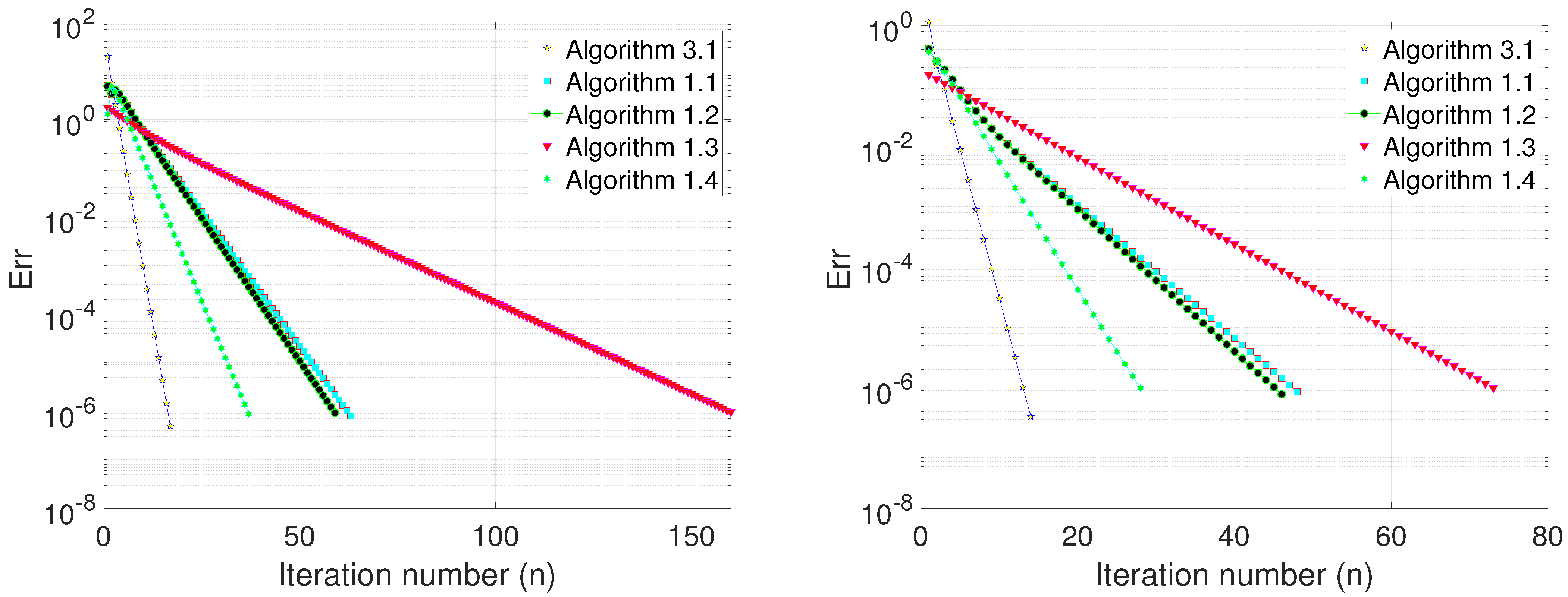
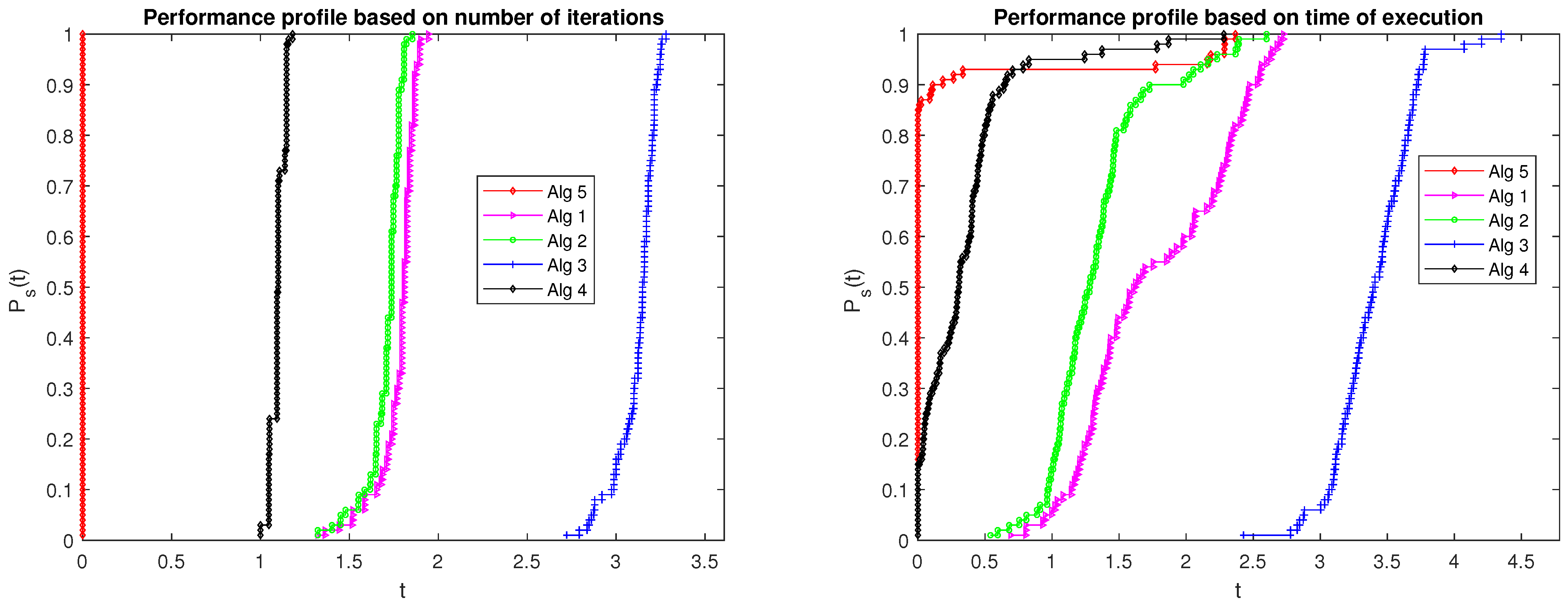
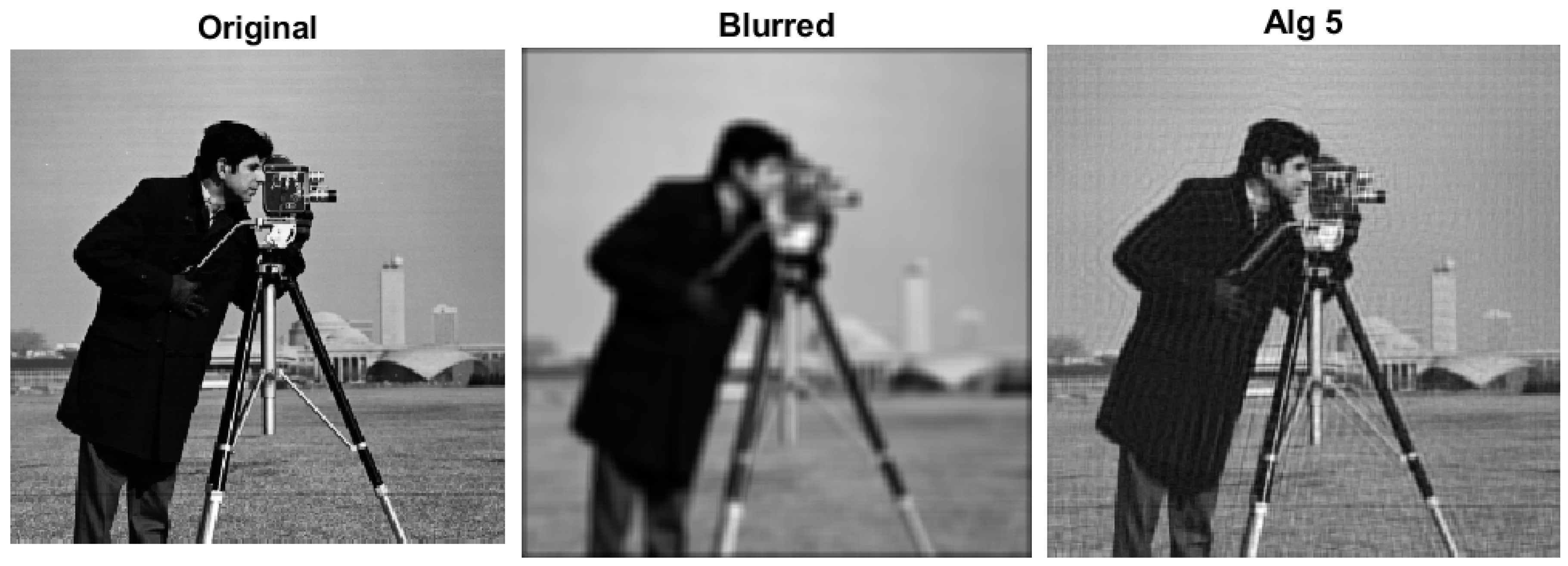
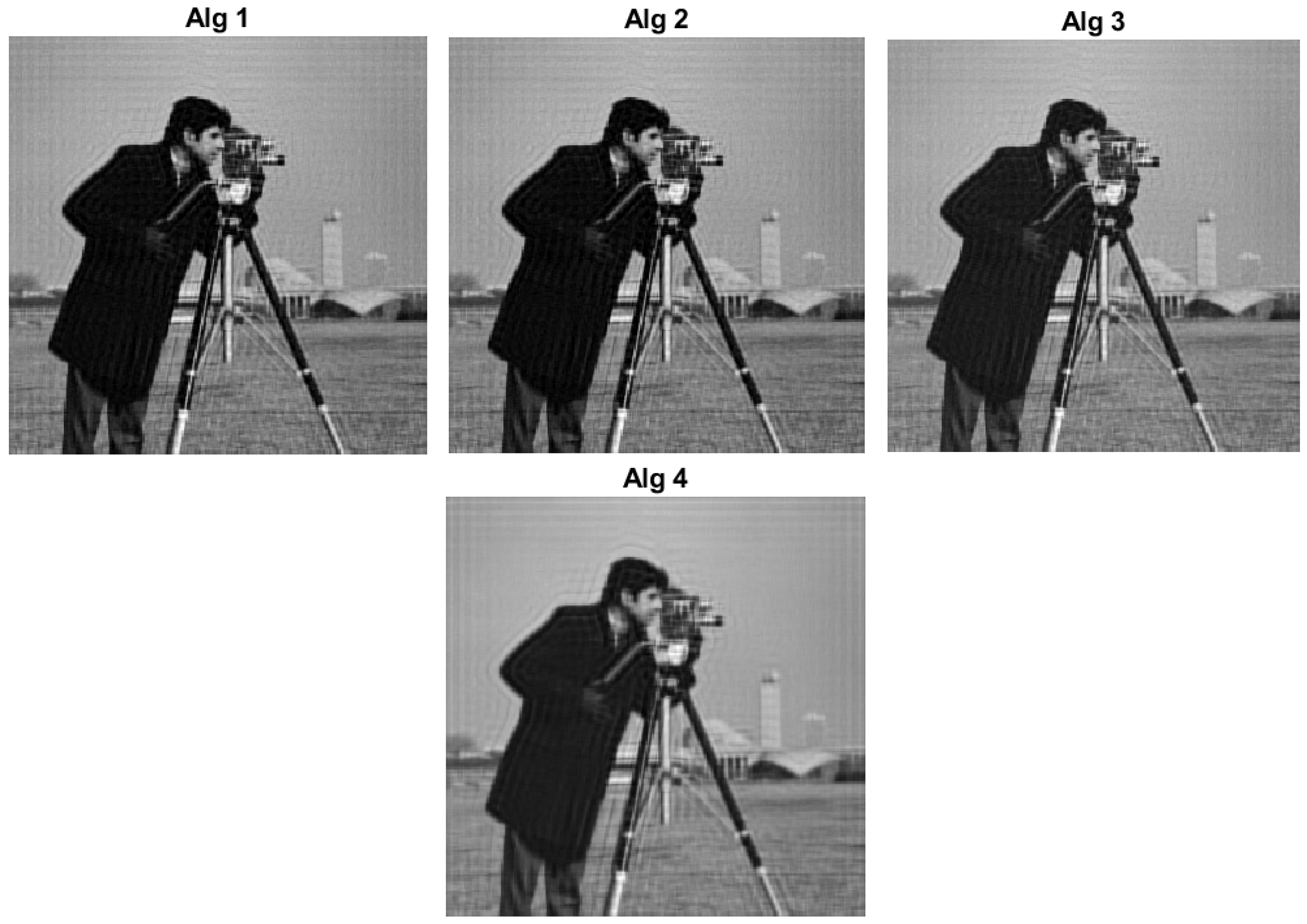
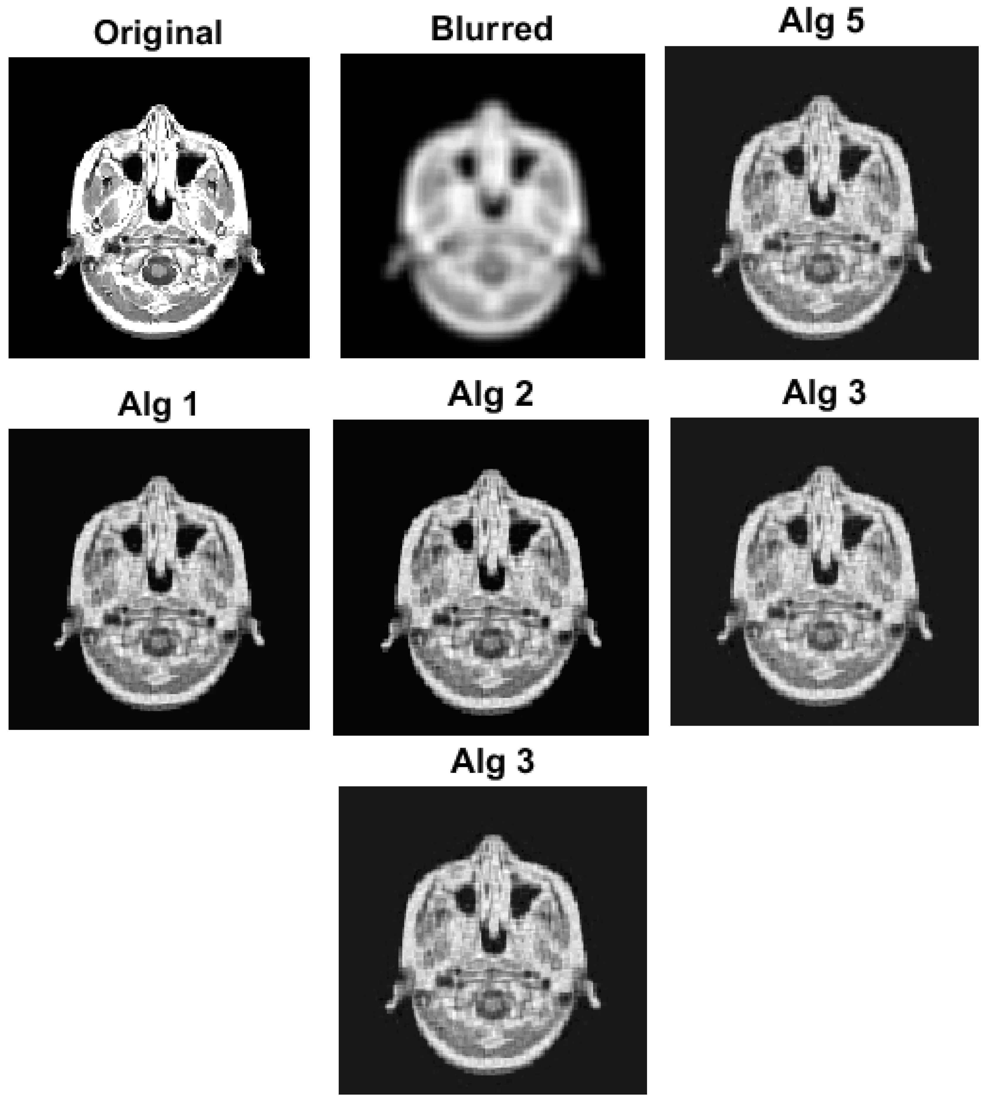
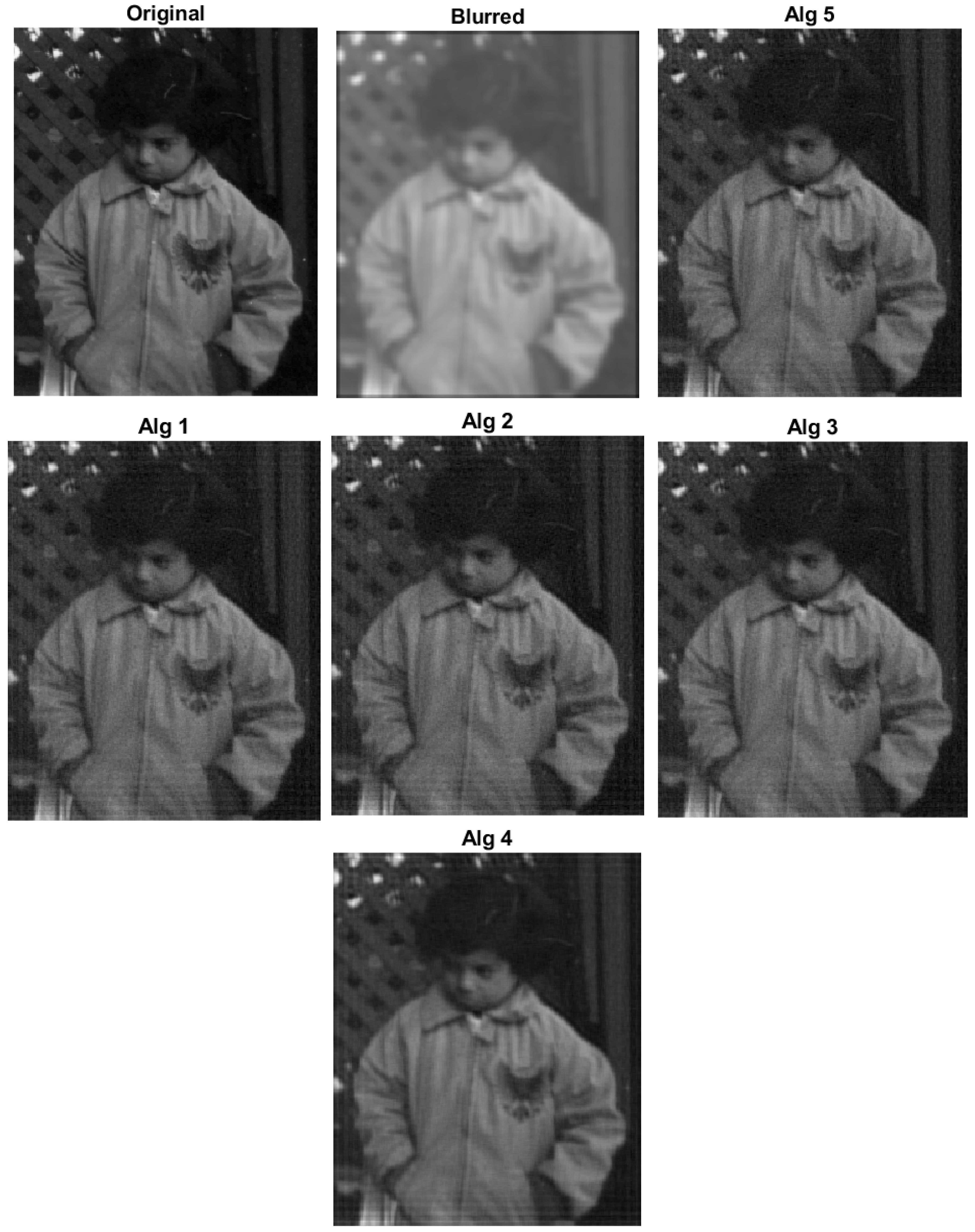
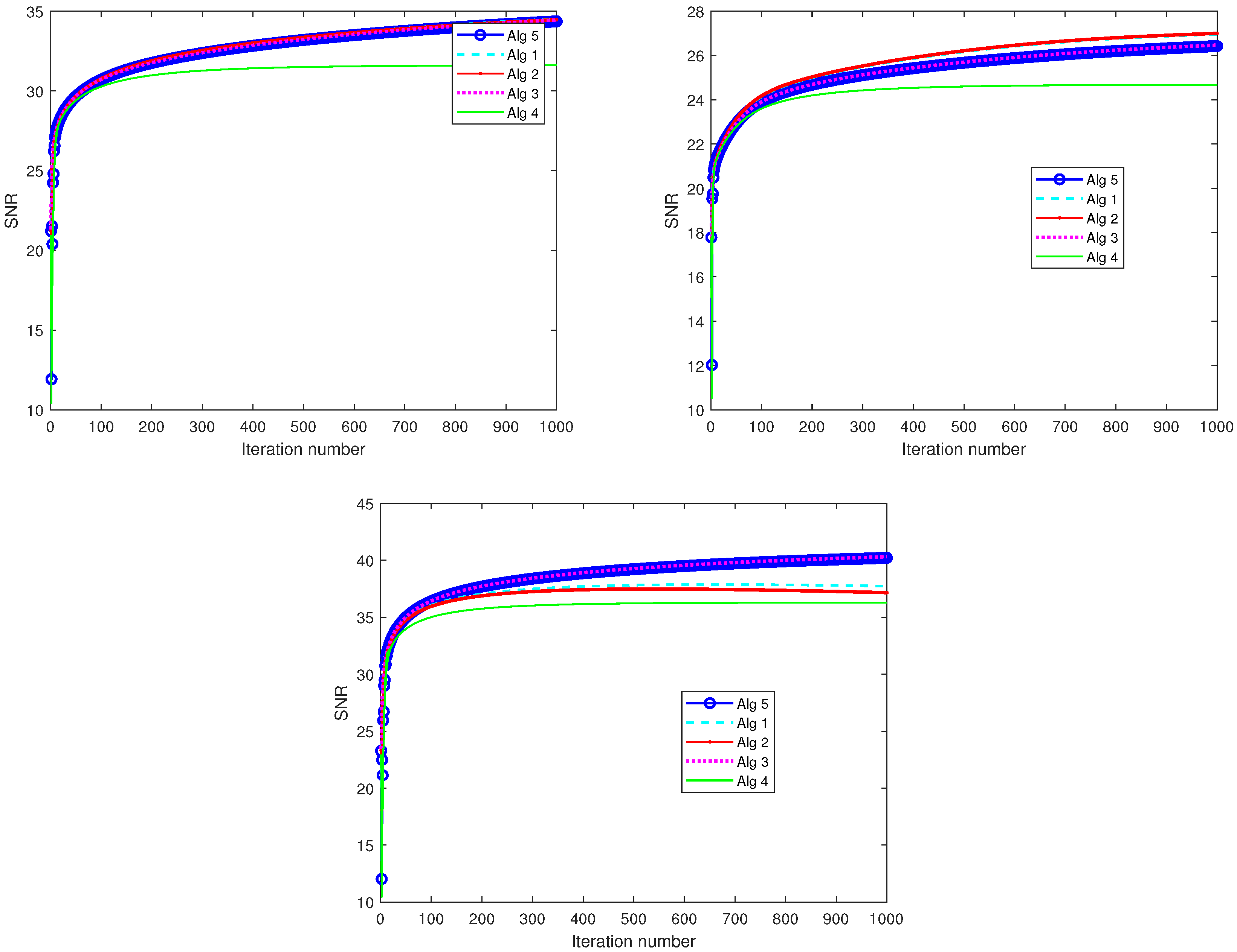
Based on the outcomes above, our paper presents a novel approach that utilizes an optimal selection of inertial term and self-adaptive techniques for solving the SVIP and fixed point problems by employing multivalued demicontractive mappings in actual Hilbert spaces. Our algorithm enhances the results of Algorithms 1–3 and 10, and other associated findings in the literature. We demonstrate a robust convergence outcome, subject to certain mild conditions, and provide relevant numerical experiments to showcase the efficiency of the proposed method. We also consider an application of our algorithm to solving image deblurring problems to demonstrate the applicability of our results.

2. Preliminaries

In this section, we present certain definitions and fundamental outcomes that will be employed in our ensuing analysis. Suppose that H is a real Hilbert space, and C is a subset of H that is closed, nonempty, and convex. We use $a_n\to p$ and $a_n\rightharpoonup p$ to denote the strong and weak convergences, respectively, of a sequence $\left\{a_n\right\}\subseteq H$ to a point $p\in H$.

For every vector $\overline{k}\in H$, there exists a unique element $P_C\overline{k}$ in the subspace C such that

$$\left|\right|P_C\left(\overline{k}\right)-\overline{k}\left|\right|=min\left\{\right||z-\overline{k}\left|\right|:z\in C\}.$$

The metric projection from H onto C is denoted as $P_C$ and can be defined by the subsequent expression:

(i)

For $\overline{k}\in H$ and $z\in C,$

$$z=P_C\left(\overline{k}\right)\iff ⟨\overline{k}-z,z-b⟩\ge 0,\forall b\in C;$$

(20)

(ii)

$⟨\overline{k}-b,P_C\left(\overline{k}\right)-P_C\left(b\right)⟩\ge \left|\right|P_C\left(\overline{k}\right)-P_C\left(b\right){\left|\right|}^2\forall \overline{k},b\in H;$

(iii)

For each $\overline{k}\in H$ and $b\in C$

$$\left|\right|b-P_C\left(\overline{k}\right){\left|\right|}^2+\left|\right|\overline{k}-P_C\left(\overline{k}\right){\left|\right|}^2\le \left|\right|\overline{k}-b{\left|\right|}^2.$$

An operator $F:H\to H$ is called:

(i)

$\alpha$-Lipschitz if there is a positive value of $\alpha$ such that

$$\left|\right|Fb-Fa\left|\right|\le \alpha \left|\right|b-a\left|\right|\forall b,a\in H$$

and a contraction if $\alpha \in (0,1)$;

(ii)

Nonexpansive if F is 1-Lipschitz;

(iii)

Quasi-nonexpansive when its fixed point set is not empty and

$$\parallel Fb-p\parallel \le \parallel b-p\parallel \forall b\in H,p\in Fix\left(F\right);$$

(iv)

$\mathit{k}$-demicontractive if $Fix\left(F\right)\ne \varnothing$ and there exists a constant $k\in [0,1)$ such that

$$\left|\right|Fa-{p\left|\right|}^2\le \left|\right|a-{p\left|\right|}^2+k\left|\right|a-{Fa\left|\right|}^2\forall a\in H,p\in Fix\left(F\right).$$

Note that the nonexpansive and quasi-nonexpansive mappings are contained in the class of $\mathit{k}$-demicontractive mapping; we also follow the same conditions for the Hausdorff mapping, $S:H\to 2^H$.

Suppose we have a metric space $(X,d)$ and a family of subsets $CB\left(X\right)$ that are both closed and bounded. We can induce the Hausdorff metric using the metric d on any two subsets $X,Y\in CB\left(X\right)$. This metric is defined as follows:

$$\mathcal{H}(X,Y)=max\left\{\underset{x\in X}{sup}d(x,Y),\underset{y\in Y}{sup}d(X,y)\right\},$$

where $d(x,Y)=\underset{y\in Y}{inf}d(x,y).$ A fixed point of a multivalued mapping $S:H\to CB\left(H\right)$ is a point $a\in H$ that belongs to $Sa.$ If $S\left(a\right)$ only contains a, then we refer to a as a strict fixed point of $S.$ The study of strictly fixed points for a specific type of contractive mappings was first conducted by Aubin and Siegel [27]. Since then, this condition has been rapidly applied to various multivalued mappings, such as those in [28,29,30].

Lemma 1. 

The inequalities stated below are valid in a Hilbert space denoted by H.:

(i) 

$\left|\right|b-{a\left|\right|}^2={\left|\right|b\left|\right|}^2-2⟨b,a⟩+{\left|\right|a\left|\right|}^2\forall b,a\in H;$

(ii) 

$\left|\right|b+{a\left|\right|}^2\le {\left|\right|b\left|\right|}^2+2⟨a,b+a⟩\forall b,a\in H.$

We also use the following Lemmas to achieve our goal in the section on the main results; Lemmas [31,32,33].

3. Main Results

In this section, we introduce our algorithm and provide its convergence analysis. First, we prove the state of our algorithm as follows:

Let $H_1,H_2$ be two real Hilbert spaces, and the multivalued maximal monotone operators are denoted by $m_i:H_i\to 2^{H_i}$, where $i=1,2$. We denote the bounded linear operator with its adjoint as $B:H_1\to H_2$ and $B^{*}:H_2\to H_1$, respectively. For $i=1,\cdots ,m$ define $S_i:H_1\to CB\left(H_1\right)$ be a finite family of ${\mathit{k}}_i$-demicontractive mappings such that $I-S_i$ is demiclosed at the point zero with $S_i\left(q\right)=\left\{q\right\}\forall q\in Fix\left(S_i\right)$ and $\mathit{k}=max\left\{{\mathit{k}}_i\right\}$. Suppose that the solution set:

$$\mathrm{\Gamma }=\{a^{*}\in H_1:0\in m_1\left(a^{*}\right),0\in m_2\left(B{a}^{*}\right)\}\cap \bigcap _{i=1}^{r}Fix\left(S_i\right)\ne \varnothing .$$

(21)

Let our contraction mapping be $g:H_1\to H_1$ with a constant of $\sigma \in (0,1)$ and $D:H_1\to H_1$ be a strongly non-negative operator with $\eta >0$ being its coefficient where this condition, $0<\xi <\frac{\eta }{\sigma }$, is satisfied. Moreover, let $\left\{{ϵ}_n\right\},\left\{{\rho }_{n,i}\right\},\left\{{\lambda }_n\right\}$ be non-negative sequences such that $0<y\le {ϵ}_n,{\rho }_{n,i},{\lambda }_n\le u<1$. Define the following functions:

$$f\left(a\right)=\frac{1}{2}\left|\right|(I-J_{\sigma }^{m_2})Ba{\left|\right|}^2$$

(22)

and

$$T\left(a\right)=B^{*}(I-J_{\lambda }^{m_2})Ba,H\left(a\right)=(I-J_{\lambda }^{m_1})a.$$

(23)

Now, we present our algorithm as follows (Algorithm 11):    

Algorithm 11 Proposed new inertial and self-adaptive method.

Step 0: Choose $\alpha >3,{\eta }_n\in (0,4)$ and select initial guess $a_0,a_1\in H_1.$ Set $n=1.$ Step 1: Choose ${\theta }_n$ such that $0\le {\theta }_n\le {\overline{\theta }}_n$, where ${\overline{\theta }}_n$ is defined below, given the $(n-1)$th and $nth$ iterates: $$\begin{array}{ccc}& {\overline{\theta }}_n& =\left\{\begin{array}{c}min\left\{\frac{n-1}{n+\alpha -1},\frac{{ϵ}_n}{max\{\parallel a_n-a_{n-1}\parallel ,n^2\parallel a_n-a_{n-1}{\parallel }^2\}}\right\}\mathrm{if}{a}_n\ne a_{n-1},\hfill \\ \frac{n-1}{n+\alpha -1}\mathrm{otherwise}.\end{array}\right.\hfill \end{array}$$ (24) Set $$v_n=a_n+{\theta }_n(a_n-a_{n-1}).$$ Step 2: Compute $${\tau }_n=\frac{{\eta }_{n}f\left(v_n\right)}{\left|\right|T\left(v_n\right){\left|\right|}^2+\left|\right|H\left(v_n\right){\left|\right|}^2}$$ and $$b_n=J_{\sigma }^{m_1}(I-{\tau }_n{B}^{*}(I-J_{\sigma }^{m_2})B)v_n$$ Step 3: Compute the next iterate via $$\left\{\begin{array}{c}{z}_n={\rho }_{n,0}{b}_n+\sum _{i=1}^r{\rho }_{n,i}{\chi }_{n,i},\hfill \\ a_{n+1}={\lambda }_n\xi g\left(a_n\right)+(1-{\lambda }_{n}D)z_n,\end{array}\right.$$ (25) where ${\chi }_{n,i}\in S_i{b}_n$ and ${\sum }_{i=1}^r{\rho }_{n,i}=1$. Set $n=n+1$ and go back to Step 1.

   To ensure our convergence outcomes, we have made assumptions on the control parameters ${\lambda }_n,{ϵ}_n,{\rho }_{n,i}$ that must meet certain conditions:

(C1)

${lim}_{n\to \infty }{\lambda }_n=0$ and ${\sum }_{n=0}^{\infty }{\lambda }_n=\infty ,$

(C2)

${lim\; inf}_{n\to \infty }({\rho }_{n,0}-\mathit{k}){\rho }_{n,i}>0\forall i=1,2,\cdots ,r,$

(C3)

${ϵ}_n=o\left({\lambda }_n\right),$ i.e., ${lim}_{n\to \infty }\frac{{ϵ}_n}{{\lambda }_n}=0.$

Remark 1. 

It is clear from (24) and Assumptions (C3), that

$$\begin{array}{c}\hfill \underset{n\to \infty }{lim}\frac{{\theta }_n}{{\lambda }_n}\parallel a_n-a_{n-1}{\parallel }^2\le \underset{n\to \infty }{lim}\frac{{\overline{\theta }}_n}{{\lambda }_n}{\parallel a_n-a_{n-1}\parallel }^2\le \underset{n\to \infty }{lim}\frac{{ϵ}_n}{{\lambda }_n}·\frac{1}{n^2}=0\end{array}$$

and

$$\underset{n\to \infty }{lim}\frac{{\theta }_n}{{\lambda }_n}\parallel a_n-a_{n-1}\parallel \le \underset{n\to \infty }{lim}\frac{{\overline{\theta }}_n}{{\lambda }_n}\parallel a_n-a_{n-1}\parallel \le \underset{n\to \infty }{lim}\frac{{ϵ}_n}{{\lambda }_n}=0.$$

Convergence Analysis

We begin the convergence of Algorithm 11 by proving the following results.

Lemma 2. 

Consider the function $f:H_2\to \mathbb{R}$ and $h:H_1\to \mathbb{R}$ defined in $\left(22\right)$; then, the functions T and H defined on $\left(23\right)$ are Lipschitz continuous.

Proof. 

Since $T\left(a\right)=B^{*}(I-J_{\sigma }^{m_2})Ba$, therefore

$$\begin{array}{ccc}\hfill \left|\right|T\left(a\right)-{T\left(b\right)\left|\right|}^2& =& ⟨B^{*}((I-J_{\sigma }^{m_2})Ba-(I-J_{\sigma }^{m_2})Bb),B^{*}((I-J_{\sigma }^{m_2})Ba-(I-J_{\sigma }^{m_2})Bb)⟩\hfill \\ & =& ⟨(I-J_{\sigma }^{m_2})(Ba-Bb),B{B}^{*}((I-J_{\sigma }^{m_2})Ba-(I-J_{\sigma }^{m_2})Bb)⟩\hfill \\ & \le & L\left|\right|(I-J_{\sigma }^{m_2})Ba-(I-J_{\sigma }^{m_2})Bb{\left|\right|}^2,\hfill \end{array}$$

(26)

where $L=\left|\right|B^{*}B\left|\right|$. On the other hand,

$$\begin{array}{ccc}\hfill ⟨T\left(a\right)-T\left(b\right),a-b⟩& =& ⟨B^{*}((I-J_{\sigma }^{m_2})Ba-(I-J_{\sigma }^{m_2})Bb),a-b⟩\hfill \\ & =& ⟨(I-J_{\sigma }^{m_2})Ba-(I-J_{\sigma }^{m_2})Bb,Ba-Bb⟩\hfill \\ & \ge & \left|\right|(I-J_{\sigma }^{m_2})Ba-(I-J_{\sigma }^{m_2})Bb{\left|\right|}^2.\hfill \end{array}$$

(27)

Combining the above formulas, we have:

$$⟨T\left(a\right)-T\left(b\right),a-b⟩\ge \frac{1}{L}\left|\right|T\left(a\right)-{T\left(b\right)\left|\right|}^2,$$

T being $\frac{1}{L}$ inverse strong monotone implies that its inverse is L-Lipschitz continuous. Furthermore,

$$⟨T\left(a\right)-T\left(b\right),a-b⟩\le \left|\right|T\left(a\right)-T\left(b\right)\left|\right|\left|\right|a-b\left|\right|,$$

hence

$$\left|\right|T\left(a\right)-T\left(b\right)\left|\right|\le L\left|\right|a-b\left|\right|.$$

Likewise, it can be observed that the function H exhibits Lipschitz continuity.    □

Lemma 3. 

The sequence $\left\{a_n\right\}$, which was generated by Algorithm 11 is bounded.

Proof. 

Given $q\in \mathrm{\Gamma }$, then

$$\begin{array}{ccc}\hfill \left|\right|v_n-q\left|\right|& =& \left|\right|a_n+{\theta }_n(a_n-a_{n-1})-q\left|\right|\hfill \\ & \le & \left|\right|a_n-q\left|\right|+{\theta }_n\left|\right|a_n-a_{n-1}\left|\right|.\hfill \end{array}$$

(28)

Since $\mathrm{\Gamma }\ne \varnothing$, then $q=J_{\sigma }^{m_1}\left(q\right)$, $Bp=J_{\sigma }^{m_2}\left(Bq\right)$, and $(I-J_{\sigma }^{m_2})Bq=Bq-Bq=0$. Note that $T\left(v_n\right)=B^{*}(I-J_{\sigma }^{m_2})B{v}_n$, $I-J_{\sigma }^{m_2}$ is firmly nonexpansive, therefore we obtain the following:

$$\begin{array}{ccc}\hfill ⟨T\left(v_n\right),v_n-q⟩& =& ⟨B^{*}(I-J_{\sigma }^{m_2})B{v}_n,v_n-q⟩\hfill \\ & =& ⟨(I-J_{\sigma }^{m_2})B{v}_n-(I-J_{\sigma }^{m_2})Bq,B{v}_n-Bq⟩\hfill \\ & \ge & \left|\right|(I-J_{\sigma }^{m_2})B{v}_n{\left|\right|}^2\hfill \\ & =& 2f\left(v_n\right)\hfill \end{array}$$

(29)

and

$$\begin{array}{ccc}\hfill \left|\right|b_n-q{\left|\right|}^2& =& \left|\right|J_{\sigma }^{m_1}(I-{\tau }_n{B}^{*}(I-J_{\sigma }^{m_2})B)v_n-q{\left|\right|}^2\hfill \\ & \le & \left|\right|(I-{\tau }_n{B}^{*}(I-J_{\sigma }^{m_2})B)v_n-q{\left|\right|}^2\hfill \\ & =& \left|\right|v_n-q-{\tau }_{n}T\left(v_n\right){\left|\right|}^2\hfill \\ & =& \left|\right|v_n-{q\left|\right|}^2+{\tau }_n^2\left|\right|T\left(v_n\right){\left|\right|}^2-2{\tau }_n⟨T\left(v_n\right),v_n-q⟩\hfill \\ & \le & \left|\right|v_n-{q\left|\right|}^2+{\tau }_n^2\left|\right|T\left(v_n\right){\left|\right|}^2-4{\tau }_{n}f\left(v_n\right)\hfill \\ & \le & \left|\right|v_n-q{\left|\right|}^2-{\eta }_n(4-{\eta }_n)\frac{f^2\left(v_n\right)}{\left|\right|T\left(v_n\right){\left|\right|}^2+\left|\right|H\left(v_n\right){\left|\right|}^2}.\hfill \end{array}$$

(30)

Since $0<{\eta }_n<4,$ then $\left|\right|b_n-q\left|\right|\le \left|\right|v_n-q\left|\right|$. We use Lemma [31] to obtain the following results:

$$\begin{array}{ccc}\hfill \left|\right|z_n-q{\left|\right|}^2& =& \left|\right|{\rho }_{n,0}{b}_n+\sum _{i=1}^r{\rho }_{n,i}{\chi }_{n,i}-q{\left|\right|}^2\hfill \\ & \le & {\rho }_{n,0}\left|\right|b_n-{q\left|\right|}^2+\sum _{i=1}^r{\rho }_{n,i}\left|\right|{\chi }_{n,i}-{q\left|\right|}^2-\sum _{i=1}^r{\rho }_{n,0}{\rho }_{n,i}\left|\right|b_n-{\chi }_{n,i}{\left|\right|}^2\hfill \\ & =& {\rho }_{n,0}\left|\right|b_n-{q\left|\right|}^2+\sum _{i=1}^r{\rho }_{n,i}d{({\chi }_{n,i},S_{i}q)}^2-\sum _{i=1}^r{\rho }_{n,0}{\rho }_{n,i}\left|\right|b_n-{\chi }_{n,i}{\left|\right|}^2\hfill \\ & \le & {\rho }_{n,0}\left|\right|b_n-{q\left|\right|}^2+\sum _{i=1}^r{\rho }_{n,i}\mathcal{H}{(S_i{b}_n,S_{i}q)}^2-\sum _{i=1}^r{\rho }_{n,0}{\rho }_{n,i}\left|\right|b_n-{\chi }_{n,i}{\left|\right|}^2\hfill \\ & \le & {\rho }_{n,0}\left|\right|b_n-{q\left|\right|}^2+\sum _{i=1}^r{\rho }_{n,i}\left(\right||b_n-{q\left|\right|}^2+{\kappa }_{i}d{(b_n,S_i{b}_n)}^2)-\sum _{i=1}^r{\rho }_{n,0}{\rho }_{n,i}\left|\right|b_n-{\chi }_{n,i}{\left|\right|}^2\hfill \\ & \le & \left|\right|b_n-{q\left|\right|}^2-\sum _{i=1}^r({\rho }_{n,0}-\kappa ){\rho }_{n,i}\left|\right|b_n-{\chi }_{n,i}{\left|\right|}^2,\hfill \end{array}$$

(31)

thus, we apply condition (C2) and have the following:

$$\left|\right|z_n-{q\left|\right|}^2\le \left|\right|b_n-q{\left|\right|}^2.$$

(32)

Follow from $\left(28\right)$, $\left(30\right)$, and $\left(31\right)$ to obtain:

$$\begin{array}{ccc}\hfill \left|\right|a_{n+1}-q\left|\right|& =& \left|\right|{\lambda }_n\left(\xi g\left(a_n\right)Dq\right)+(1-{\lambda }_{n}D)(z_n-q)\left|\right|\hfill \\ & \le & {\lambda }_n\left|\right|\xi g\left(a_n\right)-Dq\left|\right|+(1-{\lambda }_n\eta )\left|\right|z_n-q\left|\right|\hfill \\ & \le & {\lambda }_n\left[\left|\right|\xi (g\left(a_n\right)-g\left(q\right))+(\xi g\left(q\right)-Dq)\left|\right|\right]+(1-{\lambda }_n\eta )\left|\right|z_n-q\left|\right|\hfill \\ & \le & {\lambda }_n\xi \sigma \left|\right|a_n-q\left|\right|+{\lambda }_n\left|\right|\xi g\left(q\right)-Dq\left|\right|+(1-{\lambda }_n\eta )\left[\right||a_n-q\left|\right|+{\theta }_n\left|\right|a_n-a_{n-1}\left|\right|]\hfill \\ & =& (1-{\lambda }_n(\eta -\xi \sigma ))\left|\right|a_n-q\left|\right|+{\lambda }_n\left|\right|\xi g\left(q\right)-Dq\left|\right|+(1-{\lambda }_n\eta ){\sigma }_n\left|\right|a_n-a_{n-1}\left|\right|\hfill \\ & =& (1-{\lambda }_n(\eta -\xi \sigma ))\left|\right|a_n-q\left|\right|+\hfill \\ & & (\eta -\xi \sigma ){\lambda }_n\left\{\frac{\left|\right|\xi g\left(q\right)-Dq\left|\right|}{\eta -\xi \sigma }+\left(\frac{1-{\lambda }_n\eta }{\eta -\xi \sigma }\right)\frac{{\theta }_n}{{\lambda }_n}\left|\right|a_n-a_{n-1}\left|\right|\right\}.\hfill \end{array}$$

(33)

Note that ${sup}_{n\ge 1}\left(\frac{1-{\lambda }_n\eta }{\eta -\xi \sigma }\right)\frac{{\theta }_n}{{\lambda }_n}\left|\right|a_n-a_{n-1}\left|\right|$ exists by Remark 1 and let

$$M=max\left\{\frac{\left|\right|\xi g\left(q\right)-Dq\left|\right|}{\eta -\xi \sigma },\underset{n\ge 1}{sup}\left(\frac{1-{\lambda }_n\eta }{\eta -\xi \sigma }\right)\frac{{\theta }_n}{{\lambda }_n}\left|\right|a_n-a_{n-1}\left|\right|\right\}.$$

Therefore, we have the following:

$$\left|\right|a_{n+1}-q\left|\right|\le (1-{\lambda }_n(\eta -\xi \sigma ))\left|\right|a_n-q\left|\right|+{\lambda }_n(\eta -\xi \sigma )M.$$

We continue and use Lemma [32] (i) to imply that $\left\{\right||a_n-p|\left|\right\}$ is bounded and therefore, $\left\{a_n\right\}$ is also bounded. Consequently, sequences $\left\{v_n\right\}$, $\left\{z_n\right\}$, and $\left\{b_n\right\}$ are bounded.    □

Lemma 4. 

Given $\left\{a_n\right\}$ as the sequence generated by the proposed Algorithm 5, put $s_n=\left|\right|a_n-q{\left|\right|}^2$, ${\tilde{a}}_n=\frac{2{\lambda }_n(\eta -\xi \sigma )}{1-{\lambda }_n\xi \sigma }$, $u_n=\frac{1}{2(\eta -\xi \sigma )}(2⟨\xi g\left(q\right)-Dq,a_{n+1}-q⟩+{\lambda }_n{M}_1)$, for some $M_1>0$ and $c_n=\frac{{\theta }_n\left|\right|a_n-a_{n-1}\left|\right|}{1-{\lambda }_n\xi \sigma }{M}_2$ where $M_2={sup}_{n\ge 1}({(1-{\lambda }_{n}q)}^2\left(\right||a_n-q\left|\right|+\left|\right|a_{n-1}-q\left|\right|)+2{(1-{\lambda }_{n}q)}^2\left|\right|a_n-a_{n-1}\left|\right|)$ and $q\in \mathrm{\Gamma }$.

Then, the following conclusions hold:

(i) 

$s_{n+1}\le (1-{\tilde{y}}_n)s_n+c_n+{\tilde{y}}_n{u}_n$.

(ii) 

$-1\le {lim\; sup}_{n\to \infty }{u}_n<+\infty .$

Proof. 

From Algorithm 11, we have

$$\begin{array}{ccc}\hfill \left|\right|v_n-q{\left|\right|}^2& =& \left|\right|a_n+{\theta }_n(a_n-a_{n-1})-q{\left|\right|}^2\hfill \\ & =& \left|\right|a_n-{q\left|\right|}^2+2{\theta }_n⟨a_n-q,a_n-a_{n-1}⟩+{\theta }_n^2\left|\right|a_n-a_{n-1}{\left|\right|}^2.\hfill \end{array}$$

(34)

Let us use Lemma 1(i) in order to determine the following results:

$$2⟨a_n-q,a_n-a_{n-1}⟩=-\left|\right|a_{n-1}-{q\left|\right|}^2+\left|\right|a_n-{q\left|\right|}^2+\left|\right|a_n-a_{n-1}{\left|\right|}^2$$

(35)

thus, substituting $\left(35\right)$ into $\left(34\right)$, we obtain

$$\begin{array}{ccc}\hfill \left|\right|v_n-q{\left|\right|}^2& =& \left|\right|a_n-{q\left|\right|}^2+{\theta }_n(-||a_{n-1}-{q\left|\right|}^2+\left|\right|a_n-{q\left|\right|}^2+\left|\right|a_n-a_{n-1}{\left|\right|}^2)+{\theta }_n^2\left|\right|a_n-a_{n-1}{\left|\right|}^2\hfill \\ & \le & \left|\right|a_n-{q\left|\right|}^2+{\theta }_n\left(\right||a_n-{q\left|\right|}^2-\left|\right|a_{n-1}-{q\left|\right|}^2+2{\theta }_n\left|\right|a_n-a_{n-1}{\left|\right|}^2).\hfill \end{array}$$

(36)

Now, we follow from Lemma 1(ii) and have that

$$\begin{array}{ccc}\hfill \left|\right|a_{n+1}-q{\left|\right|}^2& =& \left|\right|{\lambda }_n(\xi g\left(a_n\right)-Dq)+(1-{\lambda }_{n}D)(z_n-q){\left|\right|}^2\hfill \\ & \le & {(1-{\lambda }_n\eta )}^2\left|\right|z_n-q{\left|\right|}^2+2{\lambda }_n⟨\xi g\left(a_n\right)-Dq,a_{n+1}-q⟩.\hfill \end{array}$$

(37)

Follow from $\left(30\right)$, $\left(32\right)$, and $\left(34\right)$ to obtain

$$\begin{array}{ccc}\hfill \left|\right|a_{n+1}-q{\left|\right|}^2& \le & {(1-{\lambda }_n\eta )}^2\left|\right|v_n-q{\left|\right|}^2+2{\lambda }_n⟨\xi g\left(a_n\right)-Dq,a_{n+1}-q⟩\hfill \\ & =& {(1-{\lambda }_n\eta )}^2\left(\right||a_n-{q\left|\right|}^2+{\theta }_n\left(\right||a_n-{q\left|\right|}^2-\left|\right|a_{n-1}-{q\left|\right|}^2)+2{\theta }_n\left|\right|a_n-a_{n-1}{\left|\right|}^2)+\hfill \\ & & 2{\lambda }_n⟨\xi g\left(a_n\right)-Dq,a_{n+1}-q⟩\hfill \\ & =& {(1-{\lambda }_n\eta )}^2\left|\right|a_n-{q\left|\right|}^2+{\theta }_n{(1-{\lambda }_n\eta )}^2\left(\right||a_n-{q\left|\right|}^2-\left|\right|a_{n-1}-{q\left|\right|}^2)+\hfill \\ & & 2{\theta }_n{(1-{\lambda }_n\eta )}^2\left|\right|a_n-a_{n-1}{\left|\right|}^2+2{\lambda }_n⟨\xi g\left(a_n\right)-Dq,a_{n+1}-q⟩\hfill \\ & \le & {(1-{\lambda }_n\eta )}^2\left|\right|a_n-{q\left|\right|}^2+{\theta }_n{(1-{\lambda }_n\eta )}^2\left(\right||a_n-q\left|\right|+\left|\right|a_{n-1}-q\left|\right|\left)\right||a_n-a_{n-1}\left|\right|+\hfill \\ & & 2{\theta }_n{(1-{\lambda }_n\eta )}^2\left|\right|a_n-a_{n-1}{\left|\right|}^2+2{\lambda }_n⟨\xi g\left(a_n\right)-Dq,a_{n+1}-q⟩.\hfill \end{array}$$

(38)

Also,

$$\begin{array}{ccc}\hfill 2⟨\xi g\left(a_n\right)-Dq,a_{n+1}-q⟩& =& 2⟨\xi (g\left(a_n\right)-g\left(q\right))+\xi g\left(q\right)-Dq,a_{n+1}-q⟩\hfill \\ & \le & 2\xi \sigma \left|\right|a_n-q\left|\right|\left|\right|a_{n+1}-q\left|\right|+2⟨\xi g\left(q\right)-Dq,a_{n+1}-q⟩\hfill \\ & \le & \xi \sigma \left(\right||a_n-{q\left|\right|}^2+\left|\right|a_{n+1}-{q\left|\right|}^2)+2⟨\xi g\left(q\right)-Dq,a_{n+1}-q⟩.\hfill \end{array}$$

(39)

Furthermore, substitute $\left(39\right)$ into $\left(38\right)$ and have that

$$\begin{array}{ccc}\hfill \left|\right|a_{n+1}-q{\left|\right|}^2& \le & [{(1-{\lambda }_n\eta )}^2+{\lambda }_n\xi \sigma ]\left|\right|a_n-{q\left|\right|}^2+{\theta }_n{(1-{\lambda }_n\eta )}^2\left(\right||a_n-q\left|\right|+\left|\right|a_{n-1}-q\left|\right|\left)\right||a_n-a_{n-1}\left|\right|+\hfill \\ & & 2{\theta }_n{(1-{\lambda }_n\eta )}^2\left|\right|a_n-a_{n-1}{\left|\right|}^2+{\lambda }_n\xi \sigma \left|\right|a_{n+1}-q{\left|\right|}^2+2{\lambda }_n⟨\xi g\left(q\right)-Dq,a_{n+1}-q⟩\hfill \\ & =& (1-{\lambda }_n(2q-\xi \sigma ))\left|\right|a_n-{q\left|\right|}^2+{\left({\lambda }_n\eta \right)}^2\left|\right|a_n-{q\left|\right|}^2+{\theta }_n[{(1-{\lambda }_n\eta )}^2\left(\right||a_n-q\left|\right|+\left|\right|a_{n-1}-q\left|\right|)+\hfill \\ & & 2{(1-{\lambda }_n\eta )}^2\left|\right|a_n-a_{n-1}\left|\right|\left]\right||a_n-a_{n-1}\left|\right|+{\lambda }_n\xi \sigma \left|\right|a_{n+1}-q{\left|\right|}^2+2{\lambda }_n⟨\xi g\left(q\right)-Dq,a_{n+1}-q⟩\hfill \\ & \le & (1-{\lambda }_n(2q-\xi \sigma ))\left|\right|a_n-{q\left|\right|}^2+{\lambda }_n\xi \sigma \left|\right|a_{n+1}-{q\left|\right|}^2+{\theta }_n[{(1-{\lambda }_n\eta )}^2\left(\right||a_n-q\left|\right|+\left|\right|a_{n-1}-q\left|\right|)+\hfill \\ & & 2{(1-{\lambda }_n)}^2\left|\right|a_n-a_{n-1}\left|\right|\left]\right||a_n-a_{n-1}\left|\right|+{\lambda }_n(2⟨\xi g\left(q\right)-Dq,a_{n+1}-q⟩+{\lambda }_n{M}_1)\hfill \end{array}$$

(40)

for some $M_1\ge 0$, we have that

$$\begin{array}{ccc}\hfill \left|\right|a_{n+1}-q{\left|\right|}^2& \le & \frac{(1-{\lambda }_n(2q-\xi \sigma ))}{1-{\lambda }_n\xi \sigma }\left|\right|a_n-{q\left|\right|}^2+\frac{{\theta }_n}{1-{\lambda }_n\xi \sigma }\left|\right|a_n-a_{n-1}\left|\right|M_2+\hfill \\ & & \frac{{\lambda }_n(2⟨\xi g\left(q\right)-Dq,a_{n+1}-q⟩+{\lambda }_n{M}_1)}{1-{\lambda }_n\xi \sigma }\hfill \\ & =& \left(1-\frac{2{\lambda }_n(\eta -\xi \sigma )}{1-{\lambda }_n\xi \sigma }\right)\left|\right|a_n-{q\left|\right|}^2+\frac{{\theta }_n}{1-{\lambda }_n\xi \sigma }\left|\right|a_n-a_{n-1}\left|\right|M_2\hfill \\ & & +\frac{2{\lambda }_n(\eta -\xi \sigma )}{1-{\lambda }_n\xi \sigma }\frac{(2⟨\xi g\left(q\right)-Dq,a_{n+1}-q⟩+{\lambda }_n{M}_1)}{2(\eta -\xi \sigma )}.\hfill \end{array}$$

(41)

Furthermore, from the boundedness of $\left\{a_n\right\}$, it is easy to see that

$$\underset{n\ge 0}{sup}{u}_n\le \underset{n\ge 0}{sup}\frac{1}{2(\rho -\xi \sigma )}\left(2\right||\xi g\left(q\right)-D{a}^{*}\left|\right|\left|\right|a_{n+1}-q\left|\right|+M_1)<\infty .$$

Our next objective is to demonstrate that ${lim\; sup}_{n\to \infty }{u}_n\ge -1$. To do so, we will assume the opposite and suppose that ${lim\; sup}_{n\to \infty }{u}_n<-1$, which implies that there exists $n_0\in \mathbb{N}$ where $u_n\le -1\forall n\ge n_0$. Therefore, according to (i), we can conclude that

$$\begin{array}{ccc}\hfill s_{n+1}& \le & (1-{\tilde{y}}_n)s_n+c_n+{\tilde{y}}_n{u}_n\hfill \\ & <& (1-{\tilde{y}}_n)s_n+c_n-{\tilde{y}}_n\hfill \\ & =& c_n+s_n-{\tilde{y}}_n(s_n+1)\hfill \\ & \le & c_n+s_n-2(\eta -\xi \sigma ){\lambda }_n.\hfill \end{array}$$

(42)

By induction, we obtain

$$s_{n+1}\le s_{n_0}+\sum _{i=n_0}^r{c}_i-2(\eta -\xi \sigma )\sum _{i=n_0}^r{\lambda }_i\forall n\ge n_0.$$

Taking the limit superior of both sides of the last inequality and noting that $c_i$ approaches 0, we obtain

$$\underset{n\to \infty }{lim\; sup}{s}_n\le s_{n_0}-\underset{n\to \infty }{lim}2(\eta -\xi \sigma )\sum _{i=n_0}^r{\lambda }_i=-\infty .$$

This is a contradiction of $\left\{s_n\right\}$ being a non-negative real sequence. Therefore, we can conclude that ${lim\; sup}_{n\to \infty }{u}_n\ge -1$.    □

Remark 2. 

Given that the ${lim}_{n\to \infty }{\lambda }_n\to 0$, it becomes easier to confirm that ${\tilde{y}}_n$ also approaches zero. In addition, according to Remark 1, $c_n$ approaches zero with an increasing n value.

Now, we present our strong convergence theorem.

Theorem 1. 

Given $\left\{a_n\right\}$ as the sequence generated by the proposed Algorithm 11 and suppose that Assumption (C1)–(C3) are satisfied. Then, $\left\{a_n\right\}$ strongly converges to a unique point $p=P_{\mathrm{\Gamma }}(I-D+\xi g)\left(p\right)$, which solves the variational inequality

$$⟨(D-\xi g)p,p-a⟩\le 0,a\in \mathrm{\Gamma }.$$

(43)

Proof. 

Given $q\in \mathrm{\Gamma }$. We will use ${\mathrm{\Phi }}_n$ to denote $\left|\right|a_n-q{\left|\right|}^2$. Below are the possible cases we are considering.

CASE A: We start by assuming that there exists a $n_0\in \mathbb{N}$ such that ${\mathrm{\Phi }}_n$ is monotonically decreasing $\forall n\ge n_0$. Then, ${lim}_{n\to \infty }{\mathrm{\Phi }}_n-{\mathrm{\Phi }}_{n+1}\to 0$. Our first aim is to demonstrate that ${lim}_{n\to \infty }\left\{\right||b_n-v_n\left|\right|,\left|\right|{\chi }_{n,i}-b_n\left|\right|,\left|\right|a_{n+1}-a_n\left|\right|\}\to 0$.

$$\begin{array}{ccc}\hfill \left|\right|v_n-a_n\left|\right|& =& \left|\right|a_n-a_n+{\theta }_n(a_n-a_{n-1})\left|\right|\hfill \\ & =& {\theta }_n\left|\right|a_n-a_{n-1}\left|\right|\to 0asn\to \infty ,\hfill \end{array}$$

(44)

thus, ${lim}_{n\to \infty }\left|\right|v_n-a_n\left|\right|=0$. From Equations $\left(30\right)$ and $\left(37\right)$ we have that:

$$\begin{array}{ccc}\hfill {\eta }_n(4-{\eta }_n)\frac{f^2\left(v_n\right)}{\left|\right|T\left(v_n\right){\left|\right|}^2+\left|\right|H\left(v_n\right){\left|\right|}^2}& \le & \left|\right|v_n-{q\left|\right|}^2-\left|\right|b_n-q{\left|\right|}^2\hfill \\ & \le & \left|\right|v_n-{q\left|\right|}^2-\left|\right|a_{n+1}-{q\left|\right|}^2+\left|\right|a_{n+1}-{q\left|\right|}^2-\left|\right|b_n-q{\left|\right|}^2\hfill \\ & \le & \left|\right|a_n-{q\left|\right|}^2+{\theta }_{n}M\left(\right||a_n-a_{n-1}\left|\right|)-\left|\right|a_{n+1}-{q\left|\right|}^2+(1-{\lambda }_n\tau )\left|\right|z_n-q{\left|\right|}^2+\hfill \\ & & 2{\lambda }_n⟨\xi g\left(a_n\right)-Dq,a_{n+1}-q⟩-\left|\right|b_n-q{\left|\right|}^2\hfill \\ & \le & {\mathrm{\Phi }}_n-{\mathrm{\Phi }}_{n+1}+{\theta }_{n}M\left|\right|a_n-a_{n+1}\left|\right|+\left|\right|b_n-{q\left|\right|}^2-{\lambda }_n\tau \left|\right|b_n-q{\left|\right|}^2+\hfill \\ & & 2{\lambda }_n⟨\xi g\left(a_n\right)-Dq,a_{n+1}-q⟩-\left|\right|b_n-q{\left|\right|}^2\to 0asn\to \infty .\hfill \end{array}$$

(45)

Note that $inf{\eta }_n(4-{\eta }_n)>0$ and T together with H are Lipschitz continuous, so we obtain that:

$$\underset{n\to \infty }{lim}{f}^2\left(v_n\right)=0.$$

Therefore, $f\left(v_n\right)\to 0$ and $\left|\right|b_n-v_n\left|\right|\to 0$ as $n\to \infty$. From $\left(30\right)$, $\left(31\right)$, $\left(36\right)$, and $\left(37\right)$, we obtain the following results:

$$\begin{array}{ccc}\hfill \left|\right|a_{n+1}-q{\left|\right|}^2& \le & {(1-{\lambda }_n\eta )}^2\left|\right|z_n-q{\left|\right|}^2+2{\lambda }_n⟨\xi g\left(a_n\right)-Dq,a_{n+1}-q⟩\hfill \\ & \le & {(1-{\lambda }_n\eta )}^2\left\{\left|\right|b_n-{q\left|\right|}^2-\sum _{i=1}^r({\rho }_{n,0}-\mathit{k}){\rho }_{n,i}\left|\right|b_n-{\chi }_{n,i}{\left|\right|}^2\right\}+2{\lambda }_n⟨\xi g\left(a_n\right)-Dq,a_{n+1}-q⟩\hfill \\ & \le & {(1-{\lambda }_n\eta )}^2\left\{\left|\right|a_n-{q\left|\right|}^2+{\theta }_n\left(\right||a_n-{q\left|\right|}^2-\left|\right|a_{n-1}-{q\left|\right|}^2)\right\}+{(1-{\lambda }_n\eta )}^2\hfill \\ & & \left\{2{\theta }_n\left|\right|a_n-a_{n-1}{\left|\right|}^2-\sum _{i=1}^r({\rho }_{n,0}-\mathit{k}){\rho }_{n,i}\left|\right|b_n-{\chi }_{n,i}{\left|\right|}^2\right\}+2{\lambda }_n⟨\xi g\left(a_n\right)-Dq,a_{n+1}-q⟩.\hfill \end{array}$$

(46)

Hence,

$$\begin{array}{ccc}\hfill {(1-{\lambda }_n\eta )}^2\sum _{i=1}^r({\rho }_{n,0}-\mathit{k}){\rho }_{n,i}\left|\right|b_n-{\chi }_{n,i}{\left|\right|}^2& \le & {(1-{\lambda }_n\eta )}^2\left|\right|a_n-{q\left|\right|}^2+{\theta }_n{(1-{\lambda }_n\eta )}^2\left(\right||a_n-q{\left|\right|}^2\hfill \\ & & -\left|\right|a_{n-1}-{q\left|\right|}^2)+2{\theta }_n(1-{\lambda }_n\eta )\left|\right|a_n-a_{n-1}{\left|\right|}^2\hfill \\ & & +2{\lambda }_n⟨\xi g\left(a_n\right)-Dq,a_{n+1}-q⟩-\left|\right|a_{n+1}-q{\left|\right|}^2\hfill \\ & \le & {\mathrm{\Phi }}_n-{\mathrm{\Phi }}_{n+1}+{\lambda }_n{M}_3+{\theta }_n{(1-{\lambda }_n\eta )}^2({\mathrm{\Phi }}_n-{\mathrm{\Phi }}_{n+1})\hfill \\ & & +{\theta }_n{(1-{\lambda }_n\eta )}^2\left|\right|a_n-a_{n-1}{\left|\right|}^2\hfill \\ & & +2{\lambda }_n⟨\xi g\left(a_n\right)-Dq,a_{n+1}-q⟩\to 0asn\to \infty .\hfill \end{array}$$

(47)

Thus, by applying condition (C2), we obtain

$$\underset{n\to \infty }{lim}\left|\right|b_n-{\chi }_{n,i}\left|\right|=0.$$

(48)

We also have that

$$\begin{array}{ccc}\hfill \left|\right|z_n-b_n\left|\right|& =& \left|\right|{\rho }_{n,0}{b}_n+\sum _{i=1}^r{\rho }_{n,i}{\chi }_{n,i}-b_n\left|\right|\hfill \\ & \le & {\rho }_{n,0}\left|\right|b_n-b_n\left|\right|+\sum _{i=1}^r{\rho }_{n,i}\left|\right|{\chi }_{n,i}-b_n\left|\right|\to 0,n\to \infty ,\hfill \end{array}$$

(49)

thus ${lim}_{n\to \infty }\left|\right|z_n-b_n\left|\right|=0$. Therefore,

$$\underset{n\to \infty }{lim}\left|\right|z_n-a_n\left|\right|=\underset{n\to \infty }{lim}\left(\right||z_n-b_n\left|\right|+\left|\right|b_n-a_n\left|\right|)=0.$$

Finally,

$$\begin{array}{ccc}\hfill \left|\right|a_{n+1}-z_n\left|\right|& =& \left|\right|{\lambda }_n\xi g\left(a_n\right)+(1-{\lambda }_{n}D)z_n-z_n\left|\right|\hfill \\ & =& {\lambda }_n\left|\right|\xi g\left(a_n\right)-D{z}_n\left|\right|\to 0,n\to \infty ,\hfill \end{array}$$

(50)

which results in the following:

$$\left|\right|a_{n+1}-a_n\left|\right|\le \left|\right|a_{n+1}-z_n\left|\right|+\left|\right|z_n-a_n\left|\right|\to 0asn\to \infty .$$

As $\mathit{k}\to \infty$, the subsequence $\left\{a_{n_k}\right\}$ weakly converges to $a^{*}$. Denote $F_{n_{\mathit{k}}}=I-{\tau }_{n_{\mathit{k}}}{B}^{*}(I-J_{\sigma }^{m_2})B$, since $J_{\sigma }^{m_2}$ is firmly nonexpansive, hence $F_{n_{\mathit{k}}}$ and $J_{\sigma }^{m_1}(I-{\tau }_{n_{\mathit{k}}}{B}^{*}(I-J_{\sigma }^{m_2})B)$ are averaged and nonexpansive. So the subsequence $\left\{v_{n_{\mathit{k}}}\right\}$ converges weakly to a fixed point $a^{*}$ of the operator $J_{\sigma }^{m_1}{F}_n$. We now show that $a^{*}\in \mathrm{\Gamma }$ that is $a^{*}\in m_1^{-1}\left(0\right)$ with $B{a}^{*}\in m_2^{-1}\left(0\right)$ and $a^{*}\in {\cap }_{i=1}^{r}Fix\left(S_i\right).$ From $\left(30\right)$ we have

$${\eta }_n(4-{\eta }_n)\frac{f^2\left(v_n\right)}{\left|\right|T\left(v_n\right){\left|\right|}^2+\left|\right|H\left(v_n\right){\left|\right|}^2}\le \left|\right|v_n-{q\left|\right|}^2-\left|\right|b_n-q{\left|\right|}^2,$$

since T and H are Lipschitz continuous, thus $T\left(v_n\right)$ and $H\left(v_n\right)$ are bounded. In addition, $inf{\eta }_n(4-{\eta }_n)>0$, hence $f\left(v_n\right)\to 0$ as $n\to 0$. Since the subsequence $\left\{a_{n_{\mathit{k}}}\right\}$ converges weakly to $a^{*}$, therefore, the function f is lower semi-continuous and $\parallel v_n-a_n\parallel \to 0$ as $n\to \infty$, then we can determine

$$0\le f\left(a^{*}\right)\le \underset{\mathit{k}\to \infty }{lim\; inf}f\left(v_{n_{\mathit{k}}}\right)=\underset{n\to \infty }{lim}f\left(v_n\right)=0.$$

That is,

$$f\left(a^{*}\right)=\frac{1}{2}\left|\right|(I-J_{\sigma }^{m_2})B{a}^{*}{\left|\right|}^2=0.$$

This implies that $B{a}^{*}$ is a fixed point of $J_{\sigma }^{B_2}$ or $(I-J_{\sigma }^{B_2})B{a}^{*}=0$, then we can have $B{a}^{*}\in m_2^{-1}\left(0\right)$ or $0\in m_2\left(B{a}^{*}\right)$. Moreover, the point $a^{*}$ is a fixed point of the operator $J_{\sigma }^{m_1}(I-{\tau }_n{B}^{*}(I-J_{\sigma }^{m_2})B)$, which means that $a^{*}=J_{\sigma }^{m_1}(I-{\tau }_n{B}^{*}(I-J_{\sigma }^{m_2})B)a^{*}$. Since $(I-J_{\sigma }^{m_2})B{a}^{*}=0,$ hence $(I-{\tau }_n{B}^{*}(I-J_{\sigma }^{m_2})B)a^{*}=a^{*}$, consequently $a^{*}=J_{\sigma }^{m_1}{a}^{*}$, This implies that $a^{*}$ is a stationary (fixed) point of $J_{\sigma }^{m_1}$, in fact, $a^{*}\in m_1^{-1}\left(0\right)$. Furthermore, from (48) and the fact that $I-S_i$ is demiclosed at zero, then $a^{*}\in Fix\left(S_i\right)$ for $i=1,\cdots ,r.$ Hence $a^{*}\in \mathrm{\Gamma }.$

First, we show that $\left\{a_n\right\}$ strongly converges to $a^{*}$, where $a^{*}=P_{\mathrm{\Gamma }}(I-D+\xi g)a^{*}$ is the unique solution of the variational inequality (VI):

$$⟨(D-\xi g)a^{*},a^{*}-a⟩\le 0,a\in \mathrm{\Gamma }.$$

For us to achieve our goal, we prove that ${lim\; sup}_{n\to \infty }⟨(D-\xi g)a^{*},a^{*}-a_n⟩\le 0$. Choose a subsequence $\{a_{n_j}\}$ of $\left\{a_n\right\}$ such that ${lim\; sup}_{j\to \infty }⟨(D-\xi g)a^{*},a^{*}-a_n⟩={lim}_{j\to \infty }⟨(D-\xi g)a^{*},a^{*}-a_{n_j}⟩$. Since $a_{n_j}\rightharpoonup \overline{a}$ and using (10), we have

$$\begin{array}{ccc}\hfill \underset{j\to \infty }{lim\; sup}⟨(D-\xi g)a^{*},a^{*}-a_n⟩& =& \underset{j\to \infty }{lim}⟨(D-\xi g)a^{*},a^{*}-a_{n_j}⟩\hfill \\ & =& ⟨(D-\xi g)a^{*},a^{*}-\overline{a}⟩\hfill \\ & =& ⟨a^{*}-(I-(D-\xi g))a^{*},a^{*}-\overline{a}⟩\le 0.\hfill \end{array}$$

(51)

Furthermore, we make use of Lemma 4, Lemma 4(i), and (51) to obtain that $\left|\right|a_n-a^{*}\left|\right|\to 0$, implying that sequence $\left\{a_n\right\}$ strongly converges to $a^{*}$. Case A is concluded.

CASE B: Now we assume that $\left\{\right||a_n-q|\left|\right\}$ is not monotonically decreasing. Then for some $n_0$ and $\forall n\ge n_0$, we define $\varphi :\mathbb{N}\to \mathbb{N}$ by the following:

$$\varphi \left(n\right)=max\{\mathit{t}\in \mathbb{N}:\mathit{t}\le n:{\varphi }_{\mathit{t}}\le {\varphi }_{\mathit{t}+1}\}.$$

Moreover, $\varphi$ is increasing with ${lim}_{n\to \infty }\varphi \left(n\right)\to \infty$ and

$$0\le \left|\right|a_{\varphi \left(n\right)}-q\left|\right|\le \left|\right|a_{\varphi \left(n\right)+1}-q\left|\right|,\forall n\ge n_0.$$

We can apply a similar argument to the one used in Case A and conclude that

$$\underset{n\to \infty }{lim}\left|\right|b_{\varphi \left(n\right)}-v_{\varphi \left(n\right)}\left|\right|=\underset{n\to \infty }{lim}\left|\right|x_{\varphi \left(n\right),i}-b_{\varphi \left(n\right)}\left|\right|=\underset{n\to \infty }{lim}\left|\right|a_{\varphi \left(n\right)+1}-a_{\varphi \left(n\right)}\left|\right|=0.$$

Thus, ${\mathrm{\Omega }}_v\left(a_{\varphi \left(n\right)}\right)\in \mathrm{\Gamma }$, where ${\mathrm{\Omega }}_v\left(a_{\varphi \left(n\right)}\right)$ is the weak subsequential limit of $\left\{a_{\varphi \left(n\right)}\right\}$. Also, we have

$$\underset{n\to \infty }{lim\; sup}⟨(D-\xi g)q,q-a_{\varphi \left(n\right)}⟩\le 0.$$

(52)

Thus, we follow from Lemma 4(i) and we have

$$\begin{array}{ccc}\hfill \left|\right|a_{\varphi \left(n\right)+1}-q{\left|\right|}^2& \le & \left(1-\frac{2{\lambda }_{\varphi \left(n\right)}(\eta -\xi \sigma )}{1-{\lambda }_{\varphi \left(n\right)}\xi \sigma }\right)\left|\right|a_{\varphi \left(n\right)}-q{\left|\right|}^2+\frac{2{\lambda }_{\varphi \left(n\right)}(\eta -\xi \sigma )}{1-{\lambda }_{\varphi \left(n\right)}\xi \sigma }(2⟨\xi g\left(q\right)-Dq,a_{\varphi \left(n\right)+1}-q⟩+{\lambda }_{\varphi \left(n\right)}M)+\hfill \\ & & \frac{{\alpha }_{\varphi \left(n\right)}{M}_2\left|\right|a_{\varphi \left(n\right)}-a_{\varphi \left(n\right)-1}\left|\right|}{1-{\lambda }_{\varphi \left(n\right)}\xi \sigma }\hfill \end{array}$$

(53)

for some $M>0$ and where

$$M_2=su{p}_{n\ge 1}({(1-{\lambda }_{\varphi \left(n\right)}q)}^2\left(\right||a_{\varphi \left(n\right)}-q\left|\right|+\left|\right|a_{\varphi \left(n\right)-1}-q\left|\right|)+2{(1-{\lambda }_{\varphi \left(n\right)}q)}^2\left|\right|a_{\varphi \left(n\right)}-a_{\varphi \left(n\right)-1}\left|\right|).$$

Since $\left|\right|a_{\varphi \left(n\right)}-{q\left|\right|}^2\le \left|\right|a_{\varphi \left(n\right)+1}-q{\left|\right|}^2$ then from $\left(53\right)$, we obtain the following results:

$$\begin{array}{ccc}\hfill 0& \le & \left(1-\frac{2{\lambda }_{\varphi \left(n\right)}(\eta -\xi \sigma )}{1-{\lambda }_{\varphi \left(n\right)}\xi \sigma }\right)\left|\right|a_{\varphi \left(n\right)}-q{\left|\right|}^2+\frac{2{\lambda }_{\varphi \left(n\right)}(\eta -\xi \sigma )}{1-{\lambda }_{\varphi \left(n\right)}\xi \sigma }(2⟨\xi g\left(q\right)-Dq,a_{\varphi \left(n\right)+1}-q⟩+{\lambda }_{\varphi \left(n\right)}M)+\hfill \\ & & \frac{{\alpha }_{\varphi \left(n\right)}{M}_2\left|\right|a_{\varphi \left(n\right)}-a_{\varphi \left(n\right)-1}\left|\right|}{1-{\lambda }_{\varphi \left(n\right)}\xi \sigma }-\left|\right|a_{\varphi \left(n\right)}-q{\left|\right|}^2.\hfill \end{array}$$

(54)

Hence, we obtain:

$$\begin{array}{ccc}\hfill \frac{2{\lambda }_{\varphi \left(n\right)}(\eta -\xi \sigma }{1-{\lambda }_{\varphi \left(n\right)}\xi \sigma }\left|\right|a_{\varphi \left(n\right)}-q{\left|\right|}^2& \le & \frac{2{\lambda }_{\varphi \left(n\right)}(\eta -\xi \sigma )}{1-{\lambda }_{\varphi \left(n\right)}\xi \sigma }(2⟨\xi g\left(q\right)-Dq,a_{\varphi \left(n\right)+1}-q⟩+{\lambda }_{\varphi \left(n\right)}M)+\hfill \\ & & \frac{{\alpha }_{\varphi \left(n\right)}{M}_2\left|\right|a_{\varphi \left(n\right)}-a_{\varphi \left(n\right)-1}\left|\right|}{1-{\lambda }_{\varphi \left(n\right)}\xi \sigma }.\hfill \end{array}$$

(55)

Therefore, we obtain the results below:

$$\begin{array}{ccc}\hfill \left|\right|a_{\varphi \left(n\right)}-q{\left|\right|}^2& \le & 2⟨\xi g\left(q\right)-Dq,a_{\varphi \left(n\right)+1}-q⟩+{\lambda }_{\varphi \left(n\right)}{M}_4+\frac{{\alpha }_{\varphi \left(n\right)}{M}_2\left|\right|a_{\varphi \left(n\right)}-a_{\varphi \left(n\right)-1}\left|\right|}{2{\lambda }_{\varphi \left(n\right)}(\eta -\xi \sigma )}.\hfill \end{array}$$

(56)

Since the sequence $\left\{a_{\varphi \left(n\right)}\right\}$ is bounded and ${lim}_{n\to \infty }{\lambda }_{\varphi \left(n\right)}\to 0$, it follows from Equation $\left(52\right)$ and Remark 1.

$$\underset{n\to \infty }{lim}\left|\right|a_{\varphi \left(n\right)}-q\left|\right|=0.$$

(57)

We can conclude that $\forall n\ge n_o$, the following statement holds:

$$0\le \left|\right|a_n-{q\left|\right|}^2\le max\left\{\right||a_{\varphi \left(n\right)}-{q\left|\right|}^2,\left|\right|a_{\varphi \left(n\right)+1}-{q\left|\right|}^2\}=||a_{\varphi \left(n\right)+1}-q{\left|\right|}^2.$$

Hence, ${lim}_{n\to \infty }\left|\right|a_n-q\left|\right|=0$. Therefore, we imply that sequence $\left\{a_n\right\}$ converges strongly to q. This completes the proof.    □

The result presented in Theorem 1 can lead to an improvement when compared to the findings of [26]. It is important to recall that the set of quasi-nonexpansive mappings can be classified as 0-demicontractive. Therefore, we can utilize the same discoveries to obtain outcomes when approximating a common solution for the SVIP, together with a restricted number of multivalued quasi-nonexpansive mappings. The following remark highlights our contributions to this paper:

Remark 3. 

(i) 

A new optimal choice of the inertial extrapolation technique is introduced. This can also be adapted for other iterative algorithms to perform better.

(ii) 

The algorithm obtained a strong convergence result without necessarily imposing a solid condition on the control parameters.

(iii) 

The self-adaptive technique prevents the need to calculate a prior estimate of the norm of the bounded linear operator at every iteration.

(iv) 

The algorithm produces suitable solutions that approximate the entire set of solutions Γ as stated in $\left(1\right)$, using appropriate starting points. This feature sets it apart from Tikhonov-type regularization methods, which always converge to the same solution sequence. We find this attribute particularly intriguing.

4. Numerical Illustrations

Let us provide some numerical examples that demonstrate the effectiveness and efficiency of the suggested algorithms. We will compare the performance of Algorithm 11 (also known as Algorithm 11) with Algorithms 1, 2, 3 and 10 (also known as Algorithms 1, 2, 3, and 10, respectively). Kindly note that the renumbering of the article occurred due to the change in the numbering style in the template. All codes were written in MATLAB R2020b and performed on a PC Desktop. Intel(R) Core(TM) i7-6600U CPU @ 3.00 GHz 3.00 GHz, RAM 32.00 GB.

Example 1. 

Let $H_1=H_2={\mathbb{R}}^3$ and $B,m_1,m_2:{\mathbb{R}}^3\to {\mathbb{R}}^3$ be defined by

$$B=\left(\begin{array}{ccc}1& -1& 0\\ 1& 2& 0\\ 0& 0& 3\end{array}\right),m_1=\left(\begin{array}{ccc}4& 0& 0\\ 0& 3& 0\\ 0& 0& 2\end{array}\right)\mathit{and}{m}_2=\left(\begin{array}{ccc}6& 0& 0\\ 0& 5& 0\\ 0& 0& 4\end{array}\right).$$

(58)

It is easy to check that the resolvent operators concerning $m_1$ and $m_2$ are defined by

$$J_{\sigma }^{m_1}\left(a\right)={\left(\frac{a_1}{1+4\sigma },\frac{a_2}{1+3\sigma },\frac{a_3}{1+2\sigma }\right)}^{\top }\mathit{and}{J}_{\sigma }^{m_2}\left(a\right)={\left(\frac{a_1}{1+5\sigma },\frac{a_2}{1+5\sigma },\frac{a_3}{1+4\sigma }\right)}^{\top }$$

for $\sigma >0$ and $a\in {\mathbb{R}}^3.$ Also, let $F_j:{\mathbb{R}}^3\to 2^{{\mathbb{R}}^3}$ be defined by

$$F_{j}a=\left\{\begin{array}{cc}\frac{-(3j+1)x}{3},-(j+1)a\hfill & ifa\le 0\hfill \\ -(j+1)a,\frac{-(3j+1)a}{3}\hfill & ifa>0\hfill \end{array}\right.$$

(59)

It is clear that $T\left(F\right)=\left\{0\right\}$ and $\mathcal{H}(F_{j}a,F_{j}0)={(j+1)}^2{\left|z\right|}^2.$ Thus,

$$\begin{array}{ccc}\hfill d{(a,F_{j}a)}^2& =& {\left|a+\frac{(3j+1)}{3}a\right|}^2\hfill \\ & =& {\left|\frac{(3j+4)}{3}a\right|}^2\hfill \\ & =& \left(\frac{9j^2+24j+16}{9}\right){\left|a\right|}^2.\hfill \end{array}$$

Furthermore,

$$\begin{array}{ccc}\hfill \mathcal{H}{(F_{j}a,F_{j}0)}^2& =& {(j+1)}^2{\left|a\right|}^2\hfill \\ & =& {|a-0|}^2+(j^2+2j){|a-0|}^2\hfill \\ & =& {|a-0|}^2+\frac{9j^2+2j}{9j^2+24j+16}{d}^2(a,F_{j}a).\hfill \end{array}$$

(60)

Hence, $F_j$ is $\mathit{k}$-demicontractive with $\mathit{k}=\frac{(9j^2+2j)}{9j^2+24j+16}\in \left(0.1\right)$. Moreover, the solution set $\mathrm{\Gamma }=\left\{0\right\}.$ We choose the following choice of parameters for Algorithm 11: ${\theta }_n=\frac{1}{{(n+1)}^2},{\eta }_n=\frac{2n}{5n+4},{\beta }_n=\frac{1}{m+1},{\lambda }_n=\frac{1}{n+1},\xi =1,\alpha =0,2g\left(a\right)=\frac{a}{4}D\left(a\right)=a$. For Algorithm 1, we take ${\theta }_n=\frac{2n}{5n+4},\delta =0.03;$ for Algorithm 2, we take ${\theta }_n=\frac{1}{{(n+1)}^2},$$\delta =0.04,\lambda =0.03;$ for Algorithm 3, we take ${\eta }_n=0.04$; and for Algorithm 10, we take ${\theta }_n=\frac{2n}{5n+3},{\alpha }_n=\frac{1}{n+1},{\sigma }_n=\frac{1}{2\parallel B^{*}{B\parallel }^2}.$ We test the algorithms using the following initial points:

• ([Case I:]) $a_0=$ eye(3,1) and $a_1=$ rand(3,1),
• ([Case II:]) $a_0=$ rand(3,1) and $a_1=$ rand(3,1),
• ([Case III:]) $a_0=$ randn(3,1) and $a_1=$ randn(3,1),
• ([Case IV:]) $a_0=$ ones(3,1) and $a_1=$ rand(3,1),

where “eye", “randn", “rand", and “ones" are MATLAB functions. We used $\parallel a_{n+1}-a_n\parallel <{10}^{-6}$ as the stopping criterion for all the implementation. The numerical results are shown in Table 1 and Figure 1. Furthermore, we run the algorithms for 100 randomly generated starting points to check the performance of the algorithms using the performance profile metric introduced by Dolan and More [34], which is widely accepted as a benchmark for comparing the performance of algorithms. The details of the setup of the performance profile can be found in [34]. In particular, for each algorithm $s\in \mathcal{S}=\{1,2,\cdots ,5\}$ and case $p\in \mathcal{P}=\{1,\cdots ,100\},$ we defined a parameter $t_{p,s}$ which is the computation value of algorithm $s\in \mathcal{S}$ for solving problem case $p\in \mathcal{P}$ such as the number of iterations, time of execution, or error value of Algorithm $s\in \mathcal{S}$ to solve problem $p\in \mathcal{P}$. The performance of each algorithm is scaled concerning the best performance of any other algorithm in $\mathcal{S}$, which yields the performance ratio

$${\eta }_{p,s}=\frac{t_{p,s}}{min\{t_{p,s}:s\in \mathcal{S}\}}.$$

Table 1. Numerical results for Example 1.

		Case I	Case II	Case III	Case IV
Algorithm 11	No of L.	13	15	17	14
	CPU time (s)	0.0013	0.0076	0.0090	0.0018
Algorithm 1	No of L.	43	50	63	48
	CPU time (s)	0.0282	0.0223	0.0114	0.0156
Algorithm 2	No of L.	41	48	59	46
	CPU time (s)	0.0270	0.0191	0.0137	0.0166
Algorithm 3	No of L.	104	140	160	73
	CPU time (s)	0.0305	0.0425	0.0278	0.0194
Algorithm 10	No of L.	28	32	37	28
	CPU time (s)	0.0167	0.0161	0.0148	0.0034

Figure 1. Example 1, (Top Left): Case I; (Top Right): Case II, (Bottom Left): Case III; (Bottom Right): Case IV.

We select a parameter ${\eta }_r$ such that ${\eta }_r\ge {\eta }_{p,s}$ for all p and s, and ${\eta }_{p,s}={\eta }_r$ only if solver s is unable to solve problem p. It is worth noting that the choice of ${\eta }_r$ does not affect the performance evaluation, as explained in [34]. To determine an overall assessment of each solver’s performance, we use the following measurement:

$$\begin{array}{c}\hfill P_s\left(t\right)=\frac{1}{n_p}\mathrm{size}\{p\in \mathcal{P}:{\eta }_{p,s}\le t\},\end{array}$$

the probability $P_s\left(t\right)$ represents the likelihood of solver $s\in \mathcal{S}$ to achieve a performance ratio ${\eta }_{p,s}$ within a factor $t\in \mathbb{R}$ of the best possible ratio. The performance profile $P_s:\mathbb{R}\to [0,1]$ for a solver is a non-decreasing function that is piecewise continuous from the right at each breakpoint when $P_s$ is defined as the cumulative distribution function of the performance ratio. The probability $P_s\left(1\right)$ denotes the chance of the solver achieving the best performance among all solvers. The performance profile results (Figure 2 show that Algorithm 11 has the best performance for 100% of the cases considered in terms of the number of iterations. In contrast, Algorithm 3 has the worst performance. Moreover, Algorithm 10 performs better than Algorithms 1–3 even in worst senerios. Also, Algorithm 11 has the best performance for about 82% of the cases in terms of the time of execution, followed by Algorithm 10 for about 18% of the cases. In contrast, Algorithm 3 has the worst performance in terms of the time of execution. It is good to note that despite the self-adaptive technique used in selecting the stepsize for Algorithm 3, its performance is relatively worse than other methods.

Figure 2. Performance profile results for Example 1 in terms of number of iterations (left) and time of execution (right).

Example 2. 

Our algorithms are utilized to solve an image reconstruction problem that can be modeled as the Least Absolute Selection and Shrinkage Operator (LASSO) problem described in Tibshirani’s work [35]. Alternatively, it can be modeled as an underdetermined linear system given by

$$z=ma+ϵ,$$

(61)

where a is the original image in ${\mathbb{R}}^M$, m is the blurring operator in $M\times N(M<<N$), ϵ is noise, and z is the degraded or blurred data which must be recovered. Typically, this can be reformulated as a convex unconstrained minimization problem given by

$$\begin{array}{c}\hfill \underset{a\in {\mathbb{R}}^N}{min}\left\{\frac{1}{2}{\parallel ma-z\parallel }_2^2+\lambda {\parallel a\parallel }_1\right\},\end{array}$$

(62)

where $\lambda >0,$${\parallel a\parallel }_2$ is the Euclidean norm of a and ${\parallel a\parallel }_1={\displaystyle \sum _{i=1}^N}\left|y_i\right|$ is the $l_1$-norm of a. Various scientific and engineering fields have found the problem to be a valuable tool. Over the years, several iterative techniques have been developed to solve Equation (62), with the earliest being the projection approach introduced by Figureido et al. [36]. Equivalently, the LASSO problem (62) can be expressed as an SVIP when $C=\{a\in {\mathbb{R}}^{\mathit{k}}:\parallel a{\parallel }_1\le t\}$ and $Q=\left\{z\right\}$, $m_1=\partial i_C,$$m_2=\partial i_Q,$ where $i_C$ and $i_Q$ are the indicator functions on C and Q, respectively. We aim to reconstruct the initial image a based on the information the blurred image z provides. The image is in greyscale and has a width of M pixels and a height of N pixels, with each pixel value within the $[0,255]$ range. The total number of pixels in the image is $D=M\times N.$ The signal-to-noise ratio, which is determined by the amount of noise present in the restored image, is used to evaluate the quality of the resulting image, and it is defined by

$$SNR=20\times {log}_{10}\left(\frac{{\parallel a\parallel }_2}{\parallel a-a^{*}{\parallel }_2}\right),$$

with a and $a^{*}$ being the original and restored images, respectively. In image restoration, the quality of the restored image is typically measured by its signal-to-noise ratio (SNR), where a higher SNR indicates better quality. To evaluate the effectiveness of our approach, we conducted experiments using three test images: Cameraman (256 × 256), Medical Resonance Imaging (MRI) (128 × 128), and Pout (400 × 318), all of which were obtained from the Image Processing Toolbox in MATLAB. Specifically, we degraded each test image using a Gaussian 7 × 7 blur kernel with a standard deviation of 4. We processed the algorithms using the following control parameters: Algorithm 11: ${\theta }_n=\frac{1}{n^2},{\eta }_n=\frac{2n-1}{8n+7},{\beta }_n=\frac{1}{r+1},{\lambda }_n=\frac{1}{100n+1},\xi =1,\alpha =0.4g\left(a\right)=\frac{a}{8}D\left(a\right)=2a.$ For Algorithm 1, we take ${\theta }_n=\frac{n}{7n+3},\lambda =0.05;$ for Algorithm 2, we take ${\theta }_n=\frac{1}{n^2},$$\delta =0.06,\lambda =0.09;$ for Algorithm 3, we take ${\eta }_n=0.05$; and for Algorithm 10, we take ${\theta }_n=\frac{n}{7n+3},{\alpha }_n=\frac{1}{100n+1},{\sigma }_n=\frac{1}{2\parallel B^{*}{B\parallel }^2}.$ We also choose the initial values as $a_0=\mathbf{0}\in {\mathbb{R}}^{M\times N}$ and $a_1=\mathbf{1}\in {\mathbb{R}}^{M\times N}.$ The numerical results are shown in Figure 3, Figure 4, Figure 5 and Figure 6 and Table 2. It is easy to see that all the algorithms efficiently reconstruct the blurred image. Though the performance of the algorithms varies in terms of the quality of the reconstructed image, we note that Algorithm 11 was able to reconstruct the images faster than other algorithms used in the experiments. This also emphasizes the importance of the proposed algorithm.

Figure 3. Image reconstruction using cameraman (256 × 256) image.

Figure 4. Image reconstruction using MRI (128 × 128) image.

Figure 5. Image construction using Pout image (291 × 240).

Figure 6. Graphs of SNR against iteration number. Top Left: Cameraman; Top Right: MRI; and Bottom: Pout.

Table 2. Computational result for Example 2.

Algorithms	Cameraman		MRI		Pout
	Time (s)	SNR	Time (s)	SNR	Time (s)	SNR
Algorithm 11	14.2169	34.3580	2.3627	26.4215	11.3969	40.2075
Algorithm 1	16.9989	34.3517	2.7461	26.9565	12.5370	37.7244
Algorithm 2	19.6273	34.3468	2.8171	25.8976	12.3931	40.9870
Algorithm 3	18.8111	34.4365	2.7333	26.4675	13.5479	40.3109
Algorithm 10	17.3022	31.5974	2.7074	24.6775	12.3144	36.2867

5. Conclusions

Our paper proposes a novel inertial self-adaptive iterative technique that utilizes viscosity approximation to obtain a common solution for split variational inclusion problems and fixed point problems in real Hilbert spaces. We have selected an optimal inertial extrapolation term to enhance the algorithm’s accuracy. Additionally, we incorporated a self-adaptive technique that allows for stepsize adjustment without relying on prior knowledge of the norm of the bounded linear operator. Our method has been proven to converge strongly, and we have included numerical implementations to demonstrate its efficiency and effectiveness.