Self-Organization in Randomly Forced Diffusion Systems: A Stochastic Sensitivity Technique

Abstract

The problem with the analysis of noise-induced transitions between patterns in distributed stochastic systems is considered. As a key model, we use the spatially extended dynamical “phytoplankton-herbivore” system with diffusion. We perform the parametric bifurcation analysis of this model and determine the Turing instability zone, where non-homogeneous patterns are generated by diffusion. The multistability of this deterministic model with the coexistence of several waveform pattern–attractors is found. We study how noise affects these non-homogeneous patterns and estimate the dispersion of random states using a new technique based on stochastic sensitivity function (SSF) analysis and the confidence domain method. To investigate the preferences in noise-induced transitions between patterns, we analyze and compare the results of this theoretical approach with the statistics extracted from the direct numerical simulation.

1. Introduction

Self-organization processes in physics, biology, chemistry, medicine, economics, and other fields of science have been investigated [1,2,3,4,5]. The well-known difficulties of studying self-organization in observations and experiments with real systems have resulted in the need to use mathematical modeling, computer simulation, and numerical analysis [6,7]. As a conceptual mathematical model involved in the study of the mechanisms of pattern generation, a dynamical reaction–diffusion system is usually used [8,9,10,11]. The first fundamental results that shed light on the reasons for pattern formation were in the work of Turing [12], in which self-organization was presented as a consequence of diffusion instability (Turing instability). Examples of such Turing patterns were found in biochemical systems and population dynamics [13,14,15,16].

At present, an urgent problem in the theory of self-organization is the study of the influence of random perturbations on the processes of generation and transformation of spatial structures [17,18,19,20,21,22,23]. These investigations may reveal new phenomena, even in well-studied deterministic models, exposing them from a new perspective.

Most of the results of the study of stochastic effects in spatially distributed diffusion systems have been obtained using time-consuming and costly direct numerical simulation. Under these circumstances, the development of analytical methods for studying stochastic phenomena in self-organization processes is of paramount importance.

The question of how to analytically estimate the dispersion of random states near deterministic pattern–attractors or predict the conditions under which random perturbations can transfer the system from one pattern to another remains open

In this paper, the stochastic spatially extended “phytoplankton-herbivore” model is considered. It is shown that the deterministic system in the Turing instability zone shows multistable behavior: several patterns coexist for the same parameter set. This multistability means that for different initial states, patterns of different spatial forms can be generated. Each pattern has a unique parametric domain where it remains stable.

The main focus of the paper is the study of stochastic phenomena in this model with diffusion. We show how the sensitivity to noise for pattern–attractors can be quantitatively analyzed using the stochastic sensitivity function (SSF) technique. Initially, this mathematical technique was developed for local systems (see, e.g., [24]) and is now actively used in studies of various noise-induced phenomena [25,26].

In this paper, it is demonstrated that some patterns remain relatively unchanged by random perturbations, whereas others quickly dissipate or transform into a pattern with another spatial form. We study the likelihood of noise-induced transitions between patterns. In this analysis, the important role of the relationship between the stochastic sensitivity of patterns, mutual arrangement of confidence domains, and basins of attraction is demonstrated.

2. Turing Instability and Pattern Formation

Consider the following two variable stochastic PDE systems based on the Levin–Segel model [27] with diffusion:

$$\begin{array}{c}{\displaystyle \frac{\partial u}{\partial t}=au+e{u}^2-buv+D_u\frac{{\partial }^{2}u}{\partial x^2}+\epsilon \sigma \left(x\right)\xi (t,x)}\hfill \\ {\displaystyle \frac{\partial v}{\partial t}=cuv-d{v}^2+D_v\frac{{\partial }^{2}v}{\partial x^2}+\epsilon \phi \left(x\right)\eta (t,x).}\hfill \end{array}$$

(1)

Here, the variable functions $u(t,x)$ and $v(t,x)$ represent the population densities of phytoplankton species and herbivore species, respectively. In terms of a reaction–diffusion system, the former acts as an activator (increasing value intensifies the process), and the latter acts as an inhibitor (slows down the process). The parameters a, b, c, d, and e are all considered positive: a and e stand for the nonlinear intrinsic growth rate of prey, the parameters b and c characterize the interactions of species, and the parameter d defines the intra-class competition among predators. The coefficients $D_u$ and $D_v$ are associated with the intensity of the diffusion process.

We assume that the spatial variable x varies within the domain $[0,L],L=1$. The zero-flux boundary conditions are written as

$${\displaystyle \frac{\partial u}{\partial x}(0,0)=\frac{\partial u}{\partial x}(0,1)=\frac{\partial v}{\partial x}(0,0)=\frac{\partial v}{\partial x}(0,1)=0.}$$

(2)

The stochastic components $\xi (t,x)$ and $\eta (t,x)$ are uncorrelated white Gaussian noise with the parameters:

$$\begin{array}{c}\mathrm{E}\xi (t,x)=\mathrm{E}\eta (t,x)=0,\\ \mathrm{E}\xi (t,x)\xi (t^{\prime },x^{\prime })=\delta (t^{\prime }-t)\delta (x^{\prime }-x),\\ \mathrm{E}\eta (t,x)\eta (t^{\prime },x^{\prime })=\delta (t^{\prime }-t)\delta (x^{\prime }-x).\end{array}$$

(3)

In (1), the functions $\sigma \left(x\right)$ and $\phi \left(x\right)$ allow one to model the dependence of random disturbances on the spatial variable x.

If diffusion and random noise are excluded ($D_u=D_v=0$, $\epsilon =0$), for any x there is a non-extended system with the variable functions $u\left(t\right)$ and $v\left(t\right)$. This system has two fixed points: trivial $(0,0)$ and non-trivial $\left(\frac{ad}{bc-ed},\frac{ac}{bc-ed}\right)$. In order to preserve the biological sense of the non-trivial fixed point, an additional condition $bc>ed$ must be satisfied. This equilibrium is stable if $c>e$ and unstable otherwise. The trivial equilibrium is always unstable.

In the system with diffusion, the homogeneous equilibrium is considered. In this state, for every x, the variable values are those of the fixed point of the system without diffusion. If this equilibrium is unstable in System (1), (2) with $\epsilon =0$, the diffusion instability, namely the Turing instability [12], is observed and the system will form a stable non-homogeneous state (Turing pattern). For System (1), (2) without noise ($\epsilon =0$), the condition for the Turing instability is as follows [27]:

$$\frac{D_u}{D_v}<{\left(\sqrt{\frac{b}{d}}-\sqrt{\frac{b}{d}-\frac{e}{c}}\right)}^2.$$

(4)

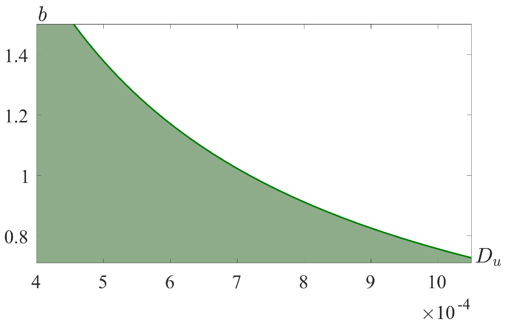
Here and subsequently, we fix $a=d=e=0.5$, $c=1$, and $D_v=0.02$, and study this system for varying b and $D_u$.

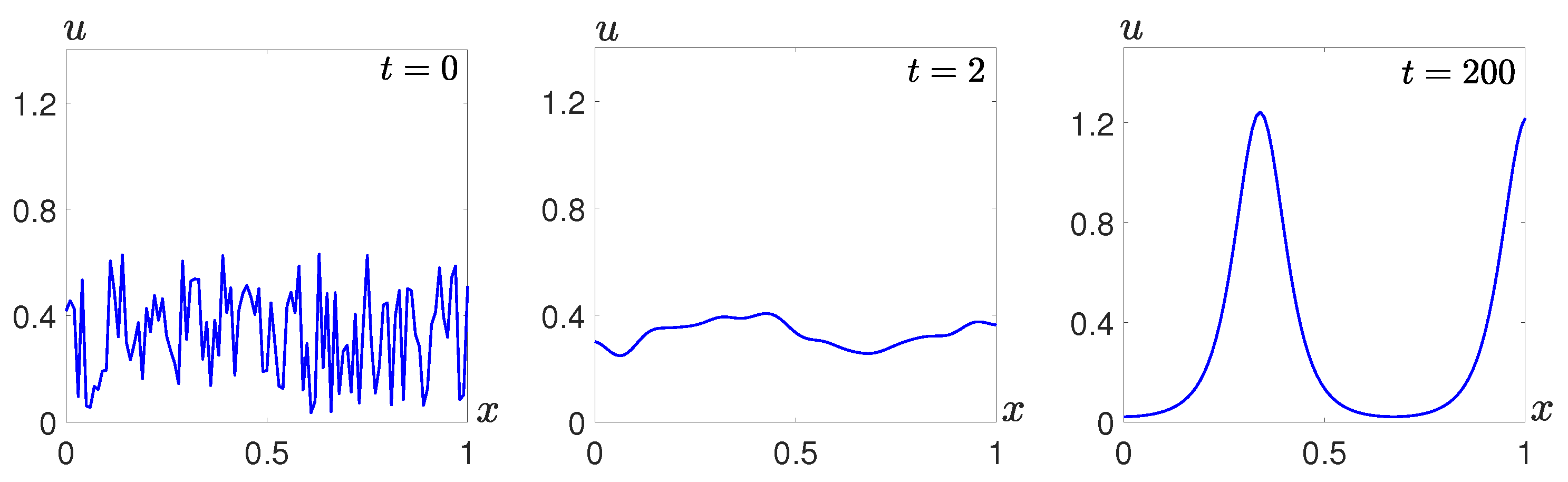
The parametric zone of the Turing instability is shown in Figure 1. Within this zone, the formation of Turing patterns is expected. An example of the process of pattern formation from the randomly generated state is demonstrated in Figure 2.

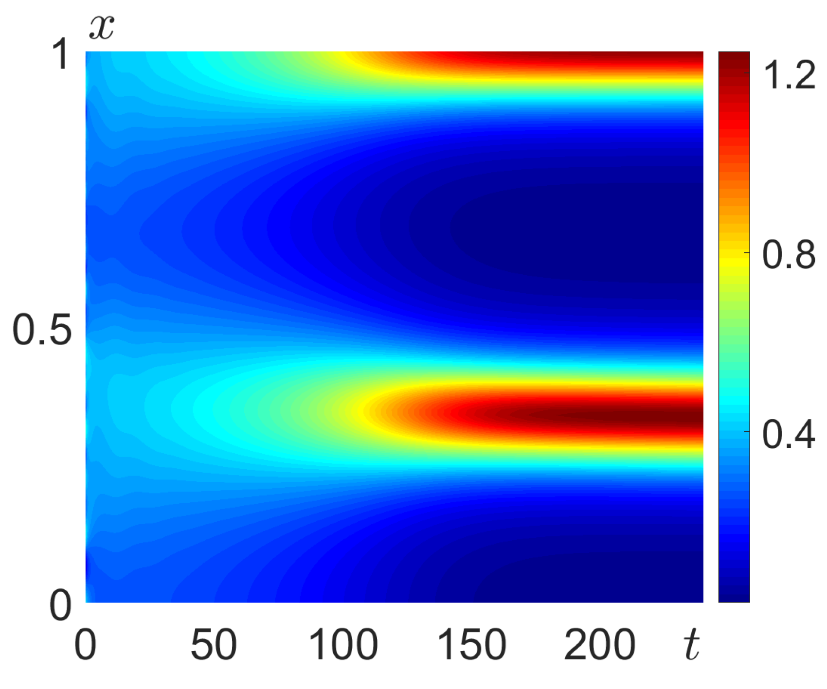
Alternatively, the evolution of the system dynamics can be visualized using heat maps. Figure 3 shows the process of pattern formation as in Figure 2. Here, the spatial variable x varies along the vertical axis, the temporal variable changes along the horizontal axis, and the color represents the value of $u(t,x)$ at the point of the spatial domain at a certain time t.

A Turing pattern resembles a wave-like structure with a specific spatial frequency (number of wavelengths within a domain). Note that due to the boundary conditions, the number of wavelengths can be either an integer or a half-integer. The tendency on the left edge of the interval can be ascending (↑) or descending (↓). Based on these properties, a pattern can be assigned a symbol, for example, the generated pattern in Figure 2 and Figure 3 would be called the $1.5\uparrow$ pattern.

3. Multistability and Stochastic Transitions

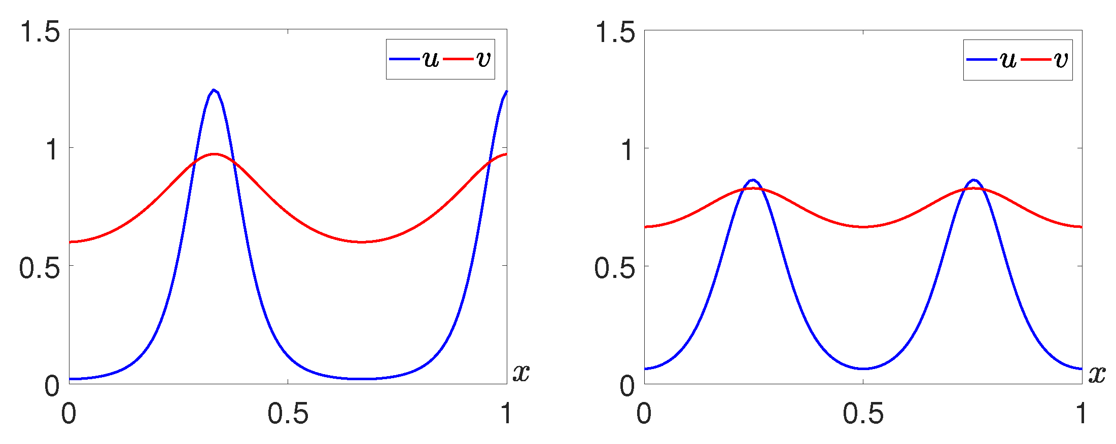
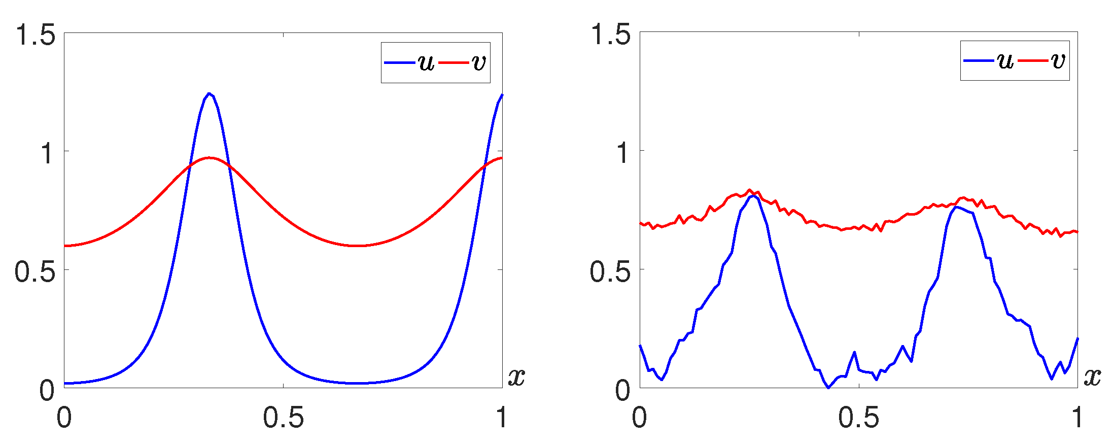
In systems of this kind, several patterns may coexist for the same set of parameter values. By altering the initial state of the system, different final states can be obtained. Figure 4 shows two patterns that were obtained for different initial conditions and the parameter values $a=d=e=0.5$, $b=c=1$, $D_u=5\times {10}^{-4}$, and $D_v=0.02$. These structures are $1.5\uparrow$ and $2\uparrow$ patterns.

Note that along with these $1.5\uparrow$ and $2\uparrow$ patterns, the system also exhibits $1.5\downarrow$ and $2\downarrow$ patterns.

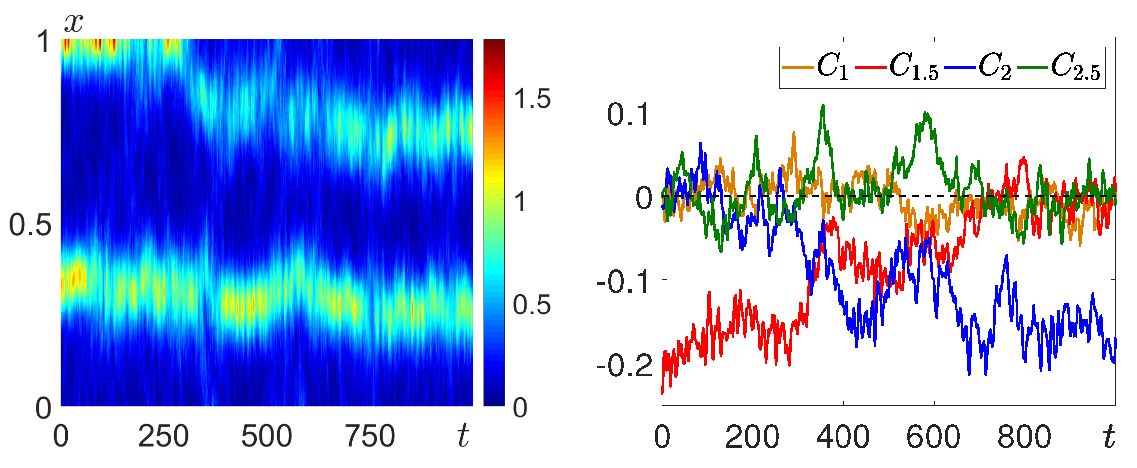
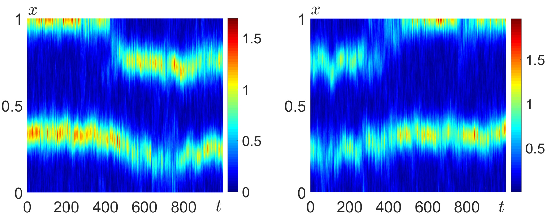
The coexistence of several stable states in these systems plays an important role in understanding stochastic behavior. It can often be seen that under the action of random perturbations, multistable systems switch from one state to another. In the spatially extended case with diffusion, noise-induced transitions between coexisting patterns can be observed. Figure 5 shows an example of when the initial deterministic $1.5\uparrow$ pattern (left) transforms under the effect of noise into a state resembling the $2\uparrow$ pattern (right).

In order to visualize the temporal dynamics, two approaches are used. The first one is the visualization of the temporal process by a heat map similar to Figure 3. However, the transition process is often difficult to distinguish by simply observing these diagrams. For more precise quantitative detection, each model state can be represented as the time series of harmonic functions $C_k\left(t\right)$:

$$C_k\left(t\right)={\int }_0^{L}u(t,x)cos\left(\frac{2\pi xk}{L}\right)dx.$$

(5)

Here, the index k is a positive integer or half-integer and the integration boundaries are the edges of the spatial domain. In a manner similar to a Fourier transformation, the value $C_k$ shows the weight of the k-periodic wave in the current state. When a pattern with k wavelengths is formed, the respective $C_k$ will have the largest absolute value, and this $C_k$ is referred to as dominant. When the transition between patterns occurs, the dominant harmonic function tends to zero and another $C_k$ becomes dominant.

The diagrams in Figure 6 demonstrate the temporal dynamics of the transition process from $1.5\uparrow$ to $2\uparrow$. Note that the absolute value of the dominant $C_{1.5}$ decreases while the absolute value of $C_2$ increases. The function $C_2$ becomes the most prominent near $t=400$ and remains so until the end of the experiment. Additionally, this approach allows the modeling software to automatically detect these transitions during numerical experiments. This is crucial during the later stages of this study, which involves the analysis of the statistically obtained data.

The possibility of transitions is related to the effect of random noise and the stochastic sensitivity of patterns. A sensitive pattern is likely to dissipate, whereas the resistant patterns remain relatively unchanged.

4. Stochastic Sensitivity Technique

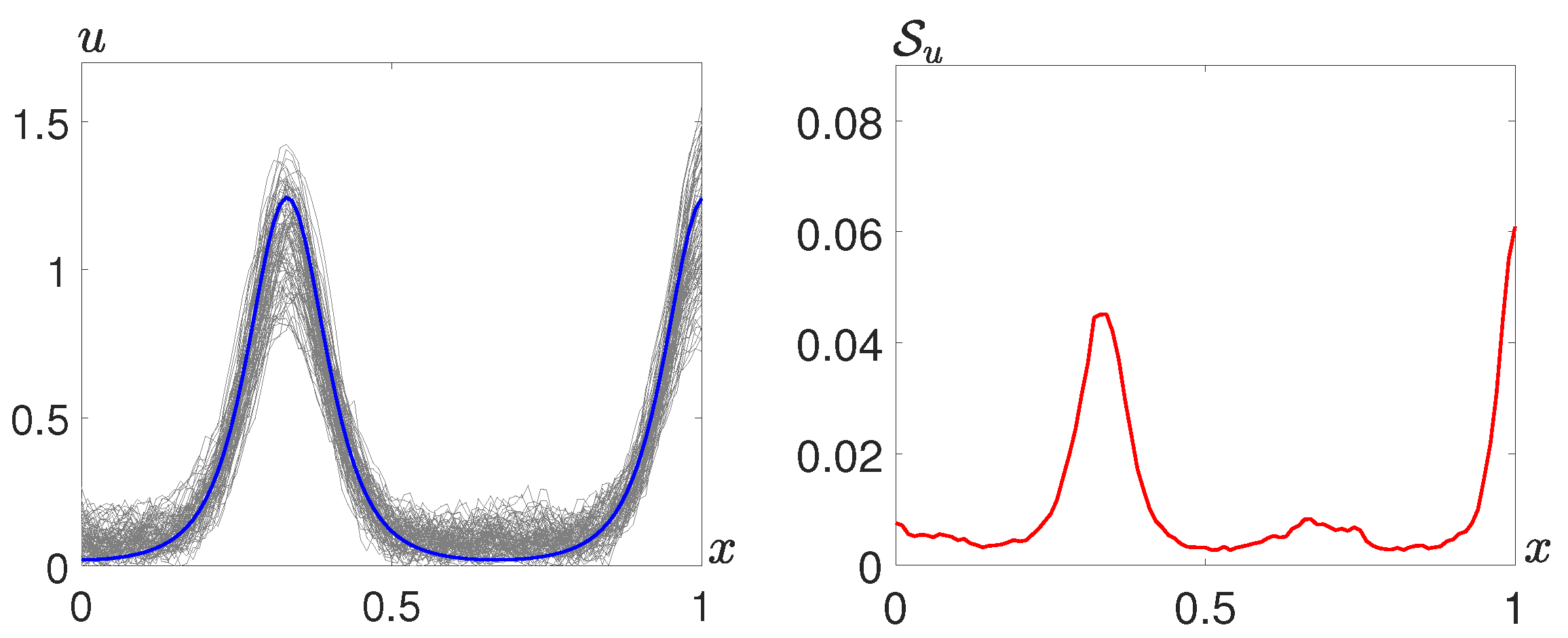
Under the effect of random noise, the system leaves the stable pattern–attractor of the deterministic model and generates a random state. The solutions form a probabilistic distribution around the initial deterministic pattern, as visualized in Figure 7 (left). The solid blue curve is the u-component of the deterministic $1.5\uparrow$ pattern. The thin gray curves show the u-components of the generated states around the deterministic pattern considered the initial state in stochastic modeling. Figure 7 (right) shows the mean-square deviation of the random states from the initial pattern for each x within the spatial domain.

The estimation of the random state distribution is the key interest of stochastic sensitivity analysis. Let $\overline{u}\left(x\right)$, $\overline{v}\left(x\right)$ describe a non-perturbed deterministic pattern of Systems (1), (2) and $u^{\epsilon }(t,x)$, $v^{\epsilon }(t,x)$ be the solutions generated by stochastic modeling with noise intensity $\epsilon$. As a measure of the dispersion of the random states $u^{\epsilon }(t,x)$, $v^{\epsilon }(t,x)$ around $\overline{u}\left(x\right)$, $\overline{v}\left(x\right)$, the mean-square deviations (6) are used:

$${\mathcal{S}}_u(x,\epsilon )=\mathrm{E}{(u^{\epsilon }(t,x)-\overline{u}\left(x\right))}^2,{\mathcal{S}}_v(x,\epsilon )=\mathrm{E}{(v^{\epsilon }(t,x)-\overline{v}\left(x\right))}^2.$$

(6)

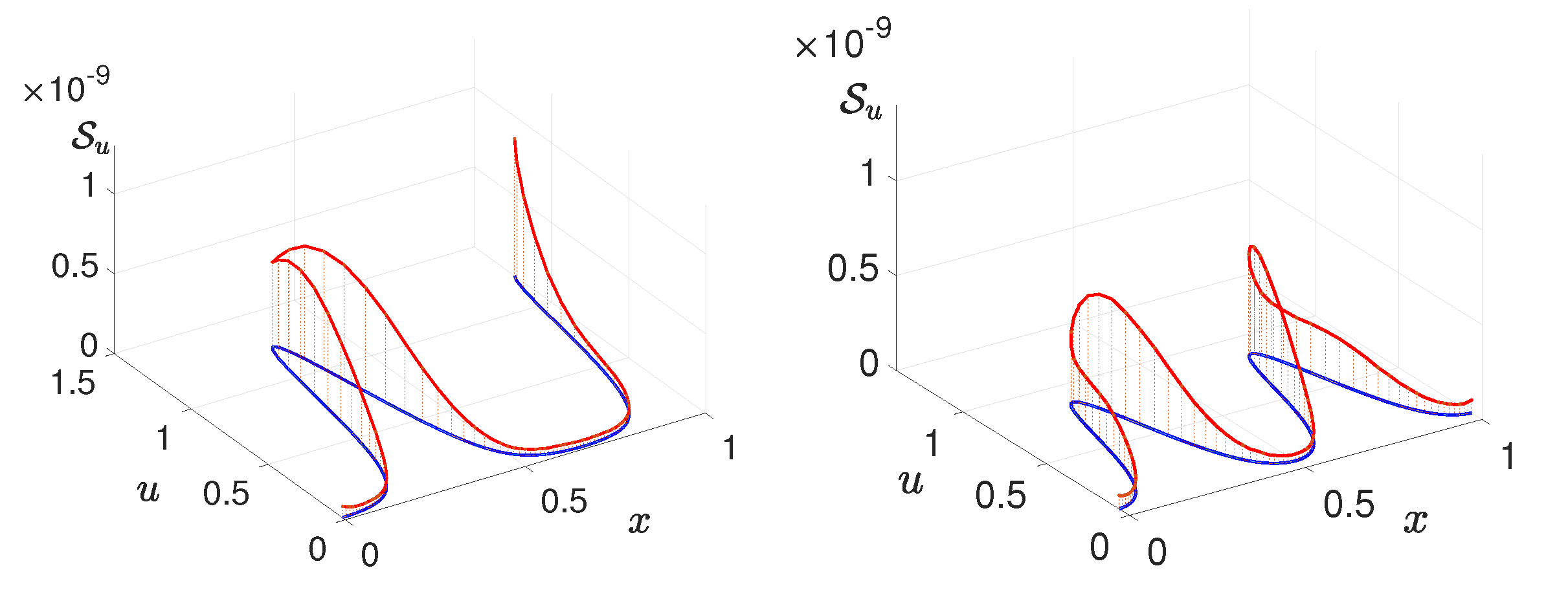
Figure 8 demonstrates the results of the statistics obtained from the numerical simulations for patterns $1.5\uparrow$ (left) and $2\uparrow$ (right), shown by blue curves. Note that ${\mathcal{S}}_u(x,\epsilon )$ (red curve) is a non-homogeneous function: the dispersion varies along the pattern. This implies that not only do different patterns show different sensitivities but also the sensitivities vary from one part of the pattern to another. In these experiments, the intensity of the random perturbations was considerably decreased in order to exclude the transitions between patterns.

The mean–square deviation of the random states from the deterministic attractor can be approximated using the stochastic sensitivity function (SSF) technique. This technique is well developed for local systems (see [24] for mathematical foundations) and is actively used to study various noise-induced phenomena [25,26].

In this technique applied to distributed systems [21], we use a discretization of the partial differential equation (PDE) system by the system of ordinary differential equations (ODE). For the corresponding ODE system, the stochastic sensitivity is defined by the matrix W, which is a unique solution of the following equation:

$$FW+W{F}^{\top }+S=0.$$

(7)

Let $x_0,x_1,\cdots ,x_{n+1}$ be the discretization of the spatial domain $[0,L]$, where $x_i=ih,h=L/(n+1)$. Denote ${\overline{u}}_i=\overline{u}\left(x_i\right)$, ${\overline{v}}_i=\overline{v}\left(x_i\right)$, where $\overline{u}\left(x\right)$, $\overline{v}\left(x\right)$ are the coordinates of the pattern–attractor of the deterministic system. For the stochastic systems (1), (2), S is an identity $2n\times 2n$-matrix and the matrix F is defined as follows:

$$\begin{array}{c}f=au+e{u}^2-buv,g=cuv-d{v}^2,\\ a_i=\frac{\partial f}{\partial u}({\overline{u}}_i,{\overline{v}}_i),\alpha =\frac{D_u}{h^2},m_i=\frac{\partial g}{\partial v}({\overline{u}}_i,{\overline{v}}_i),\beta =\frac{D_v}{h^2},\\ B=diag[b_1,...,b_n],b_i=\frac{\partial f}{\partial v}({\overline{u}}_i,{\overline{v}}_i),\\ Q=diag[q_1,...,q_n],q_i=\frac{\partial g}{\partial v}({\overline{u}}_i,{\overline{v}}_i),\\ F=\left[\begin{array}{cc}A& B\\ Q& M\end{array}\right],\end{array}$$

(8)

$$A=\left[\begin{array}{ccccccc}{a}_1-{\alpha }_1& {\alpha }_1& 0& \cdots & 0& 0& 0\\ {\alpha }_2& a_2-2{\alpha }_2& {\alpha }_2& \cdots & 0& 0& 0\\ 0& {\alpha }_3& a_3-2{\alpha }_3& \cdots & 0& 0& 0\\ \cdots & \cdots & \cdots & \cdots & \cdots & \cdots & \cdots \\ 0& 0& 0& \cdots & {\alpha }_{n-1}& a_{n-1}-2{\alpha }_{n-1}& {\alpha }_{n-1}\\ 0& 0& 0& \cdots & 0& {\alpha }_n& a_n-{\alpha }_n\end{array}\right],$$

$$M=\left[\begin{array}{ccccccc}{m}_1-{\beta }_1& {\beta }_1& 0& \cdots & 0& 0& 0\\ {\beta }_2& m_2-2{\beta }_2& {\beta }_2& \cdots & 0& 0& 0\\ 0& {\beta }_3& m_3-2{\beta }_3& \cdots & 0& 0& 0\\ \cdots & \cdots & \cdots & \cdots & \cdots & \cdots & \cdots \\ 0& 0& 0& \cdots & {\beta }_{n-1}& m_{n-1}-2{\beta }_{n-1}& {\beta }_{n-1}\\ 0& 0& 0& \cdots & 0& {\beta }_n& m_n-{\beta }_n\end{array}\right].$$

Using the matrix W, one can obtain the stochastic sensitivity of the pattern–attractor $(\overline{u}\left(x\right),\overline{v}\left(x\right))$ at the points $x_i$:

$$\begin{array}{c}{\mathcal{W}}_u\left(x_i\right)=W_{i,i}i=1,2,\cdots ,n\hfill \\ {\mathcal{W}}_v\left(x_i\right)=W_{i,i}i=n+1,n+2,\cdots ,2n.\hfill \end{array}$$

(9)

These functions can then be used to approximate the mean-square deviation of the random states around the attractor as follows:

$$\begin{array}{cc}& {\mathcal{S}}_u(x,\epsilon )\approx {\overline{\mathcal{S}}}_u(x,\epsilon )={\epsilon }^2{\mathcal{W}}_u\left(x\right),\\ & {\mathcal{S}}_v(x,\epsilon )\approx {\overline{\mathcal{S}}}_v(x,\epsilon )={\epsilon }^2{\mathcal{W}}_v\left(x\right).\end{array}$$

(10)

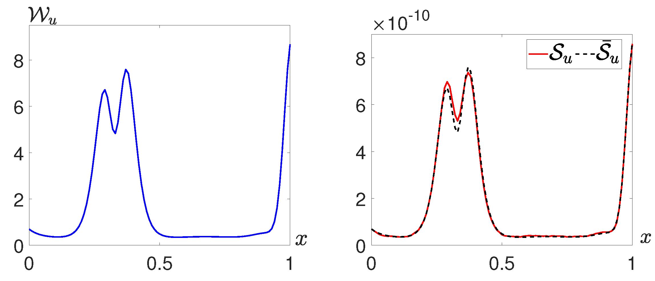
Figure 9 shows an example of the SSF ${\mathcal{W}}_u$ (left) for a $1.5\uparrow$ pattern and estimation ${\overline{\mathcal{S}}}_u$ of the mean-square deviation ${\mathcal{S}}_u$ (right) for the noise intensity $\epsilon ={10}^{-5}$. Note that the estimation ${\overline{\mathcal{S}}}_u$ found at the base of the SSF technique agrees well with the statistically acquired data.

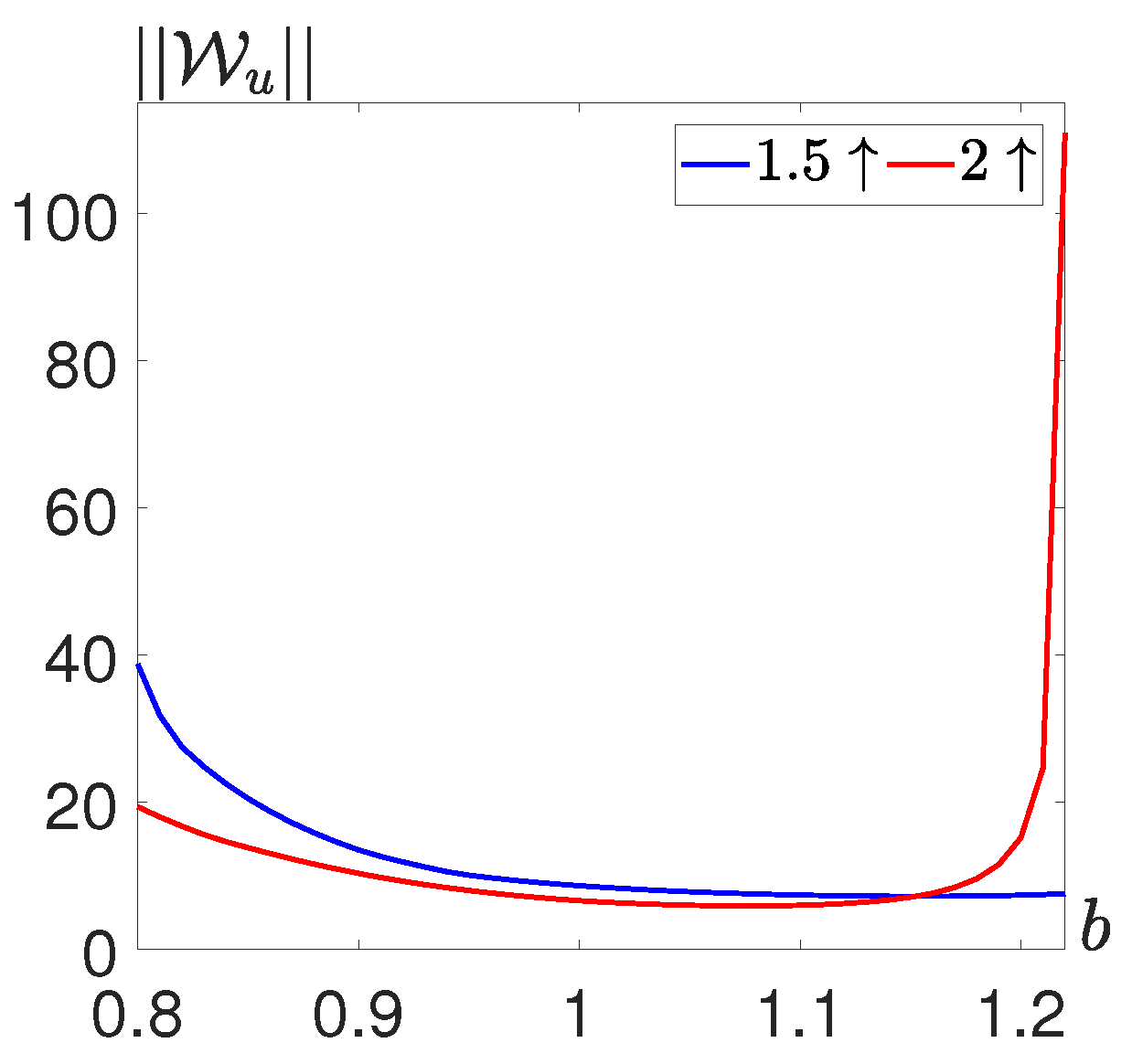
For visualization, comparison, and parametric analysis of the stochastic sensitivity, it is often useful to have a numeric measure, for example, a $C^0$-norm: $\left|\right|{\mathcal{W}}_u\left|\right|=max|{\mathcal{W}}_u\left(x_i\right)|$. Figure 10 shows how this metric changes under the variation of the parameter b for $1.5\uparrow$ and $2\uparrow$ patterns. Note that near $b=1.2$, the stochastic sensitivity of the $2\uparrow$ pattern rapidly grows, unlike the $1.5\uparrow$ pattern.

When the difference in the stochastic sensitivity becomes significant, the more sensitive pattern is more likely to break, whereas the less sensitive pattern remains stable. In this case, a stochastic transition from one pattern to another is expected.

5. SSF Technique in the Analysis of Stochastic Transitions between Patterns

The main point of interest in this work is the application of the SSF to the analysis and prediction of noise-induced transitions between patterns. In systems without diffusion, the connection between the noise-induced transitions, stochastic sensitivity of attractors, and configuration of their basins of attraction has long been studied. When there are multiple attractors, the state of the system can stay within one basin of attraction or leave it to end up in another basin of attraction. In this case, the SSF is used to build confidence regions around attractors. Noise-induced transitions between attractors are considered possible if the confidence region around one attractor intersects with the basins of other attractors.

In order to apply the same idea to the analysis of noise-induced transitions in spatially extended systems, additional information about the basins of attraction is required. These basins are too complex to build and visualize, even if discretization of the continuous system is used. However, they can still be roughly estimated and compared.

In the following example, the initial state for the numerical simulation is formed as the point of the interval connecting two coexisting deterministic patterns $1.5\uparrow$ and $2\uparrow$. The $1.5\uparrow$ pattern is defined by the functions $u_{1.5}\left(x\right)$, $v_{1.5}\left(x\right)$, and the $2\uparrow$ pattern is defined by $u_2\left(x\right)$, $v_2\left(x\right)$. We consider the linear combinations (11) as the initial states for the experiments, with the parameter k varying within $[0,1]$:

$$\begin{array}{cc}u(0,x)& =k{u}_{1.5}\left(x\right)+(1-k)u_2\left(x\right),\\ v(0,x)& =k{v}_{1.5}\left(x\right)+(1-k)v_2\left(x\right).\end{array}$$

(11)

Note that for $k=0$, the initial state is exactly the $2\uparrow$ pattern, and for $k=1$, it is the $1.5\uparrow$ pattern. The parameter k is varied and for each experiment after the transient process ($t=1000$), the Euclidean distance between the solution of the deterministic system and both patterns is measured. 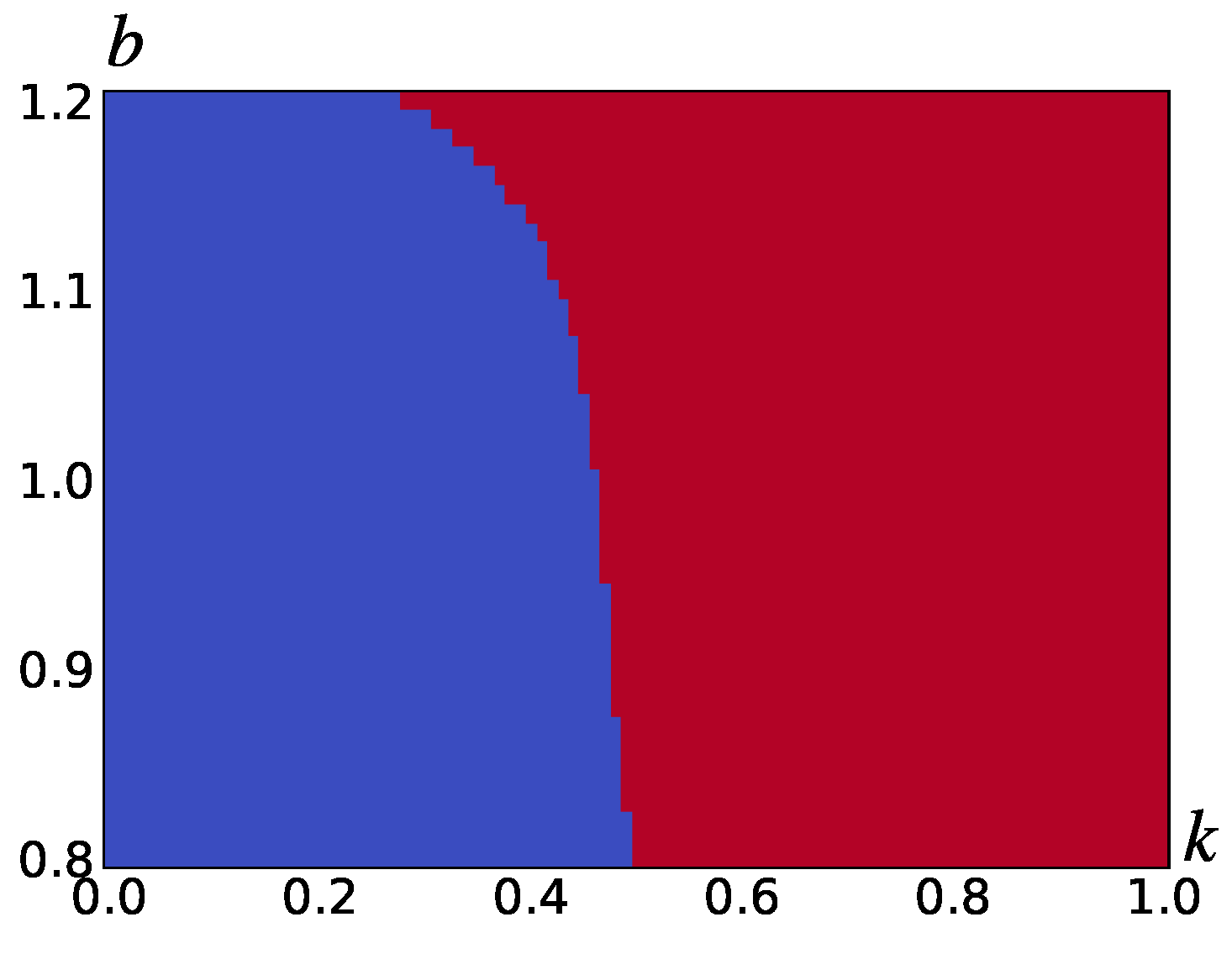If the final state is closer to $2\uparrow$, then k is marked in blue, and if it is near $1.5\uparrow$, then k is marked in red. The results of our numerical experiments are presented in Figure 11 in the plane $(k,b)$. This figure allows one to compare the basins of the $1.5\uparrow$ (red) and $2\uparrow$ (blue) patterns in this multi-dimensional system.

This deterministic analysis shows that the basin of attraction for the $1.5\uparrow$ pattern is wider than that for the $2\uparrow$ pattern. This, in turn, implies that a randomly generated state is likely to tend toward the $1.5\uparrow$ pattern. For greater values of parameter b, the basin of the $2\uparrow$ pattern shrinks. The critical k values form an approximate border between the basins of the two patterns.

In the analysis of the noise-induced transitions between the patterns, one should take into account a mutual arrangement of attraction basins and confidence domains. In the stochastically forced system, the mean-square deviation $\mathcal{D}$ of a random state from the deterministic pattern in the direction of the unit vector c can be estimated as

$$\mathcal{D}={\epsilon }^2{c}^{\top }Wc.$$

(12)

Here, $\epsilon$ is the noise intensity and W is the stochastic sensitivity matrix of the pattern–attractor.

By the $3\sigma$ rule, a random state will end up within the $3\sigma$-interval in the direction of c with a probability of 0.997 for $\sigma =\sqrt{\mathcal{D}}$. Using this rule, one can estimate the critical value ${\epsilon }_{\mathcal{A}}$ corresponding to the onset of noise-induced transitions from the basin of attraction of pattern $\mathcal{A}$ to the basin of attraction of another pattern, $\mathcal{B}$. It is assumed that for this noise magnitude ${\epsilon }_{\mathcal{A}}$, the confidence interval for pattern $\mathcal{A}$ touches the border between the basins of attraction of coexisting patterns. Let r be the Euclidean distance between patterns $\mathcal{A}$ and $\mathcal{B}$ and $k^{*}$ be the value of k that marks the separating point. The curve $k^{*}\left(b\right)$ is seen in Figure 11 as the border between the blue and red domains. This critical value ${\epsilon }_{\mathcal{A}}$ can be estimated as

$${\epsilon }_{\mathcal{A}}=\frac{r{k}^{*}}{3\sqrt{c^{\top }{W}_{\mathcal{A}}c}}.$$

(13)

Here, c is the unit vector collinear to the straight line connecting patterns $\mathcal{A}$ and $\mathcal{B}$.

A comparison of the critical noise intensities for patterns $\mathcal{A}=1.5\uparrow$ and $\mathcal{B}=2\uparrow$ under consideration is given in

Table 1. Critical noise intensity values for $1.5\uparrow$ pattern (${\epsilon }_{1.5\uparrow }$) and $2\uparrow$ pattern (${\epsilon }_{2\uparrow }$) in Systems (1), (2) with $a=d=e=0.5$, $c=1$, $D_u=5\times {10}^{-4}$, and $D_v=0.02$.

b	${\mathit{k}}^{*}$	${\mathit{\epsilon }}_{1.5\uparrow }$	${\mathit{\epsilon }}_{2\uparrow }$
1.0	0.46	0.154	0.107
1.1	0.42	0.103	0.052
1.2	0.29	0.056	0.009

for three values of b. To some extent, this correlates with Figure 10, where the sensitivity values appear comparable for lower values of the parameter b. For greater values of b, there is a significant difference in the stochastic sensitivity. In Figure 11, a similar result is demonstrated: the sizes of the attraction basins are similar for $b=0.8$ ($k^{*}\approx 0.49$), and for $b>1.1$, the boundary between the basins moves toward the $2\uparrow$ pattern, making its attraction domain narrower.

In general, this critical value decreases as the system parameters are moved toward the Turing boundary, which should indeed affect pattern stability. Note that lower values of the critical noise intensity imply that patterns are more easily broken. To verify this technique, we performed a series of statistical experiments. For $b=1$, $b=1.1$, and $b=1.2$, each of the patterns $1.5\uparrow$ and $2\uparrow$ is taken as the initial state for the numerical simulations with varying noise intensity. In each iteration using the harmonic coefficients (5), we find the most dominant spatial periodicity. Initially, it corresponds to the initial pattern as $C_{1.5}$ or $C_2$ will have the largest absolute value. If the coefficient $C_k$ loses dominance, the pattern is considered dissipated due to either a transition process or destruction by noise of a large magnitude. If during the calculations there is no loss of dominance until $t=1000$, it is assumed that the pattern resisted the influence of the noise and the deviations were insignificant.

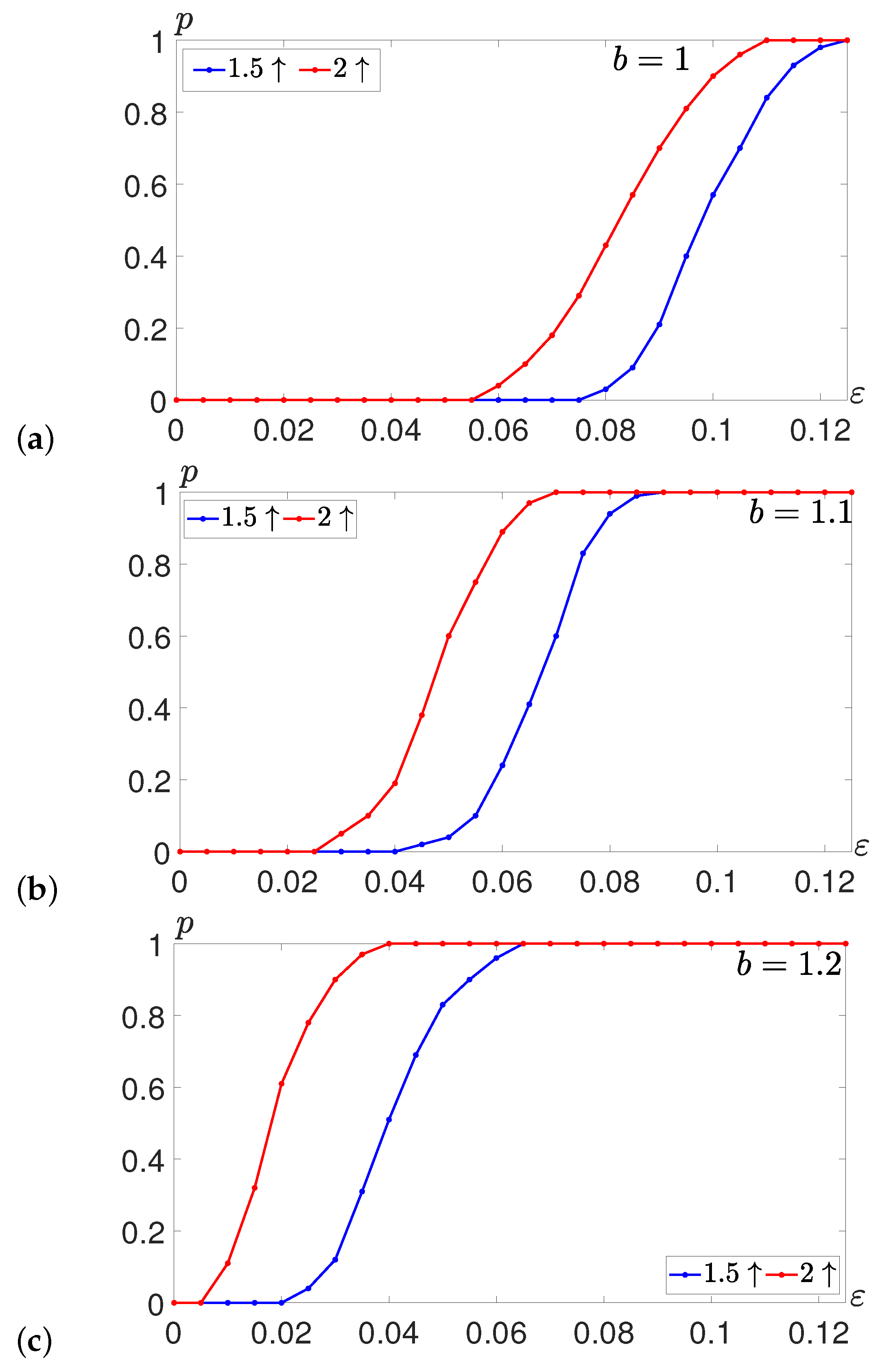
Figure 12 shows the results of this experiment. Here, the probability of pattern destruction is displayed for the aforementioned values of b versus the noise intensity $\epsilon$. This probability is shown in blue for the $1.5\uparrow$ pattern and red for the $2\uparrow$ pattern.

The results show that with the increase in b, the minimal $\epsilon$ for which the patterns begin to dissipate decreases. Additionally, the $2\uparrow$ pattern generally deteriorates more often compared to $1.5\uparrow$. In the case of $b=1$, for the noise magnitude $\epsilon \approx 0.08$, the harmonic coefficient $C_2$ loses dominance slightly earlier. For $b=1.1$ and $b=1.2$, this difference in the destruction rates becomes more significant. Transitions from the $2\uparrow$ pattern to the more stable $1.5\uparrow$ pattern are expected. The precision of the provided estimation method is difficult to evaluate, however, it can still be applied to observe the general tendency and give predictions.

For example, let $b=1$ and $\epsilon =0.1$. According to Table 1, the destruction of the $2\uparrow$ pattern should be almost certain ($\epsilon \approx {\epsilon }_{2\uparrow }=0.107$). As for the $1.5\uparrow$ pattern, the loss of dominance is not certain but probable to occur because $\epsilon$ is comparable with ${\epsilon }_{1.5\uparrow }\approx 0.15$. The results of direct modeling in Figure 13 show that transitions may occur in both directions: $2\uparrow \to 1.5\uparrow$ and $1.5\uparrow \to 2\uparrow$. This is also supported by the statistical data (see Figure 12a): the probability of the destruction of the $2\uparrow$ pattern is close to one and the $1.5\uparrow$ pattern is destroyed in more than half of the numerical experiments.

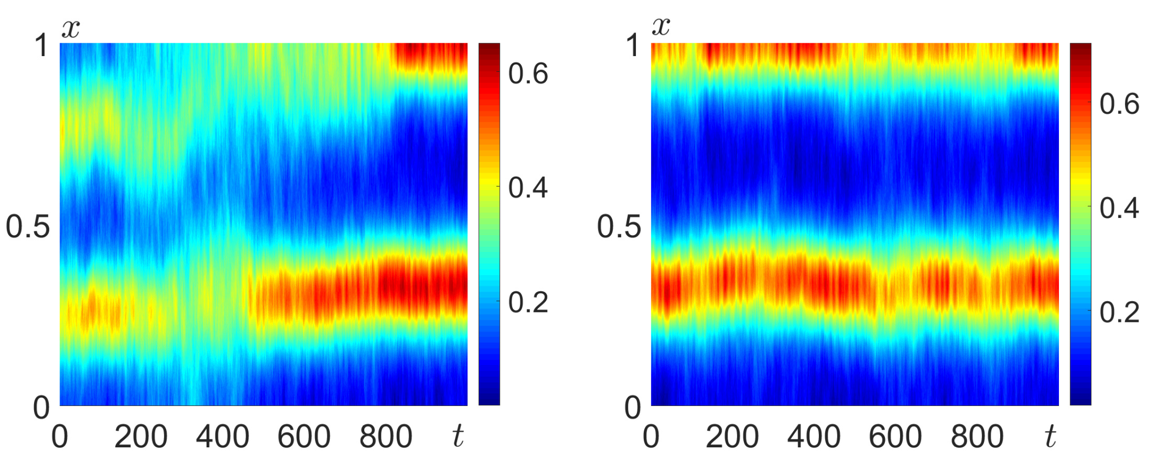
Another example is shown in Figure 14 for $b=1.2$, $\epsilon =0.02$. Note that for this b, the critical values of the noise intensity are ${\epsilon }_{1.5\uparrow }\approx 0.009$ and ${\epsilon }_{2\uparrow }\approx 0.056$. This difference in the critical values is essential so for $\epsilon =0.02$, the $2\uparrow$ pattern is expected to be destroyed, whereas the $1.5\uparrow$ pattern is expected to remain relatively resistant. These scenarios of noise-induced transitions predicted by the SSF technique and confidence domain method are justified by the direct numerical simulation in Figure 14. Indeed, this noise causes $2\uparrow \to 1.5\uparrow$ (left), whereas the $1.5\uparrow$ pattern is resistant to noise of this intensity. This can be also seen in Figure 12c: the probability of the destruction of the $1.5\uparrow$ pattern is almost zero, whereas for the $2\uparrow$ pattern, this probability is approximately 0.6. Therefore, only unidirectional transitions $2\uparrow \to 1.5\uparrow$ are expected here.

6. Conclusions

In this paper, we considered the pattern formation mechanisms for a spatially extended population dynamical model with diffusion and random perturbations. Under stochastic forcing, a probabilistic distribution of the random states is generated surrounding the deterministic pattern–attractors. The stochastic sensitivity function technique is applied to study the deviation of the random states from the pattern. The efficiency of the method is demonstrated by a comparison with the statistical data obtained from the direct numerical simulation. It is shown that the initial deterministic diffusion model exhibits multistability, with the coexistence of several pattern–attractors with different waveforms. In our study, the main focus is on the phenomenon of noise-induced transitions between coexisting patterns in this multistable system. For quantitative analysis of the stochastic transitions, the harmonic coefficients are used. For the study of the noise-induced transitions between attractors and their preferences, we propose an analytical technique, taking into account the size of basins and stochastic sensitivity of coexisting pattern–attractors. Based on this technique, one can evaluate the critical intensity of the noise at which a certain pattern is likely to dissipate. If the critical value of the noise intensity is significantly higher for one pattern than for another one, the unidirectional stochastic transitions are probable. Note that the described method is useful in studies of stochastic transitions in other, more general, multistable diffusion systems.