Spatially Weighted Bayesian Classification of Spatio-Temporal Areal Data Based on Gaussian-Hidden Markov Models

Abstract

This article is concerned with an original approach to generative classification of spatiotemporal areal (or lattice) data based on implementation of spatial weighting to Hidden Markov Models (HMMs). In the framework of this approach data model at each areal unit is specified by conditionally independent Gaussian observations and first-order Markov chain for labels and call it local HMM. The proposed classification is based on modification of conventional HMM by the implementation of spatially weighted estimators of local HMMs parameters. We focus on classification rules based on Bayes discriminant function (BDF) with plugged in the spatially weighted parameter estimators obtained from the labeled training sample. For each local HMM, the estimators of regression coefficients and variances and two types of transition probabilities are used in two levels (higher and lower) of spatial weighting. The average accuracy rate (ACC) and balanced accuracy rate (BAC), computed from confusion matrices evaluated from a test sample, are used as performance measures of classifiers. The proposed methodology is illustrated for simulated data and for real dataset, i.e., annual death rate data collected by the Institute of Hygiene of the Republic of Lithuania from the 60 municipalities in the period from 2001 to 2019. Critical comparison of proposed classifiers is done. The experimental results showed that classifiers based on HMM with higher level of spatial weighting in majority cases have advantage in spatial–temporal consistency and classification accuracy over one with lower level of spatial weighting.

1. Introduction

This article is concerned with a generative approach (see, e.g., [1]) to supervised classification of spatiotemporal data collected at fixed areal units (sites, locations) and specified by HMMs with continuous observations in each class (state) and traditionally invoked conditional independence assumption for observation distribution and Markov assumption for label transition probabilities (see, e.g., [2]). That is an extension to the basic HMM when observation may be signified by continuous real value instead of discrete value. We focus on the models that describes the process of randomly generating an unobservable class label (state) sequences from the first-order Markov chain and generating an Gaussian observation from each class to produce an observable sequence from single probabilistic distribution [3,4]. Unlike the conventional conditional density HMM, the proposed HMMs consider the temporal information of each areal unit obtain the most possible sequence of label by the incorporating the spatial information through spatial weights. It should be noted that HMM with spatial weighting have been successfully used in land-cover classification [5]. Shekhar [6], Atkinson [7], Tang et al. [8] extended pixel-based geostatistically weighted classifiers to object-based image classifications. Kadhem, Hewson, and Kaimi [9] developed Poisson HMM to model spatial dependence in network. However, only the cases with geostatistical models of observation based on spatial covariances or semivariograms are considered there.

Comprehensive literature survey on state-of-the-art advances in spatiotemporal data analysis is proposed by Ali Hamdi et al. [10]. Systematic review of methods in spatial deep learning is reported by Mishra et al. [11]. It should be noted that in the environmental agricultural and other research, data are often collected across space and through time. The spatiotemporal data are usually recorded at regular time intervals (time lags) and at irregular stations (areas) in compact area (see, e.g., [12,13]). Modeling and prediction of a such type of data has been studied by the numerous authors (see, e.g., [14,15,16,17]). Often before analyzing spatiotemporal datasets, spatiotemporal discretization (or aggregation) is applied. The discretization is useful to summarize information and help in extracting features within a spatiotemporal range rather than measuring a single point [18]. Compared with the general classification problem, spatial classification needs to consider the location information of the data and the interaction among feature and label variables at every time moment. There are currently a variety of ways to achieve the classification goal, but one of the most effective one is to use the BDF. The generative approach to spatial classification is studied by numerous authors (see, e.g., [19,20,21,22]). The approach to Bayesian classification of Gaussian Markov Random Fields (GMRF) observation on the lattice has been developed by Dreižienė and Dučinskas [23,24,25], and generative classification method for geostatistical spatiotemporal Gaussian model is introduced by Karaliutė and Dučinskas [26,27].

Novelty of our approach lies in the incorporation of spatial weights in HMM parameter estimation from labeled training sample and using plug-in BDF for classification (decoding) of the test observation. This enables us to enrich and generalize the existed generative classification methods of spatiotemporal data modeled by HMM.

Our approach is aimed at situation when BDF is implemented for data that are collected at fixed areal units (or sites as they are also known) over the fixed sequential time periods. At the beginning, for each local HMM, the maximum likelihood estimators of regression coefficients and variances and two types of transition probabilities estimators are derived from labeled training sample.

Furthermore, HMM parameter estimators in two spatial weighting levels are plugged in BDF. Two levels of spatial weighting are specified as follows:

• lower level called as partial spatial weighting (PSW) indicates that parameter estimators of Gaussian component are spatially weighted when transition probability estimators remain unweighted;
• higher level called as complete spatial weighting (CSW) comprise the cases with spatially weighted estimators of Gaussian parameters and transition probabilities.

Performance measure of the classifier are chosen to be the ACC and BAC evaluated from the confusion matrices for a test sample. The proposed methodology is illustrated for simulated data and for real dataset, i.e., annual death rate data collected by the Institute of Hygiene of the Republic of Lithuania from the 60 municipalities in the period from 2001 to 2019. Presented critical comparison of proposed classifier by the introduced criteria with existing ones can aid in the selection of proper classification rules of spatiotemporal areal data.

The experimental results showed that proposed HMM in CSW level in majority cases have advantage in classification accuracy over HMM in PCW level by both performance measures.

In order to carry out the study, this paper is organized as follows. First, Section 2 introduces the HMM for spatial–temporal Gaussian data. Next, Section 3 introduces Bayesian classification based on HMM, while Section 4 compares them by two criteria via simulation. In Section 5, we offer a real application of our approach of classification of annual death rate data collected by the Institute of Hygiene of the Republic of Lithuania from the 60 municipalities in the period from 2001 to 2019. Finally, conclusions and comments are made in the last section.

2. HMM for Spatiotemporal Data

Formally, we identify the set of possible labels of classes (e.g., diseases, land cover labels, etc.) as $\Omega =\{0,1\}$ across n areal units over T years in the time series. Let $S=\{s_i\in D;i=1,\dots ,n\}$ be a set of n nonoverlapping areal units (AUs). Assume that S is endowed with a neighborhood system $N=\{N_i:i=1,\dots ,n\}$, where $N_i$ denotes the collection of areas that are neighbors of area $s_i$. Usually, the neighborhood $N_i$ could be defined to be those areas with which area $s_i$ shares a common border. For each area unit $s_i$, data consist of feature variable observation $Z(s_i,t)$ (further simply observation) and label $Y(s_i,t)\in \Omega$ observed at consecutive time periods at $t=1,2,\dots$. Let $|N_i|$ denote number of elements in the set $N_i$.

Furthermore, use the following notation $Y(s_i,t)=Y_t^{(i)},Z(s_i,t)=Z_t^{(i)}$, for $i=1,\dots ,n$ and $t=1,\dots ,T+1$.

In this study, we assume that for $l=0,1$, the model of observation $Z_t^{(i)}$conditional on $Y_t^{(i)}=l$ is

$$Z_t^{(i)}={\mu }_l(s_i;t)+{\epsilon }_t^{(i)},$$

where ${\mu }_l(s_i;t)$ is deterministic spatiotemporal mean and errors ${\epsilon }_1^{(i)},\dots ,{\epsilon }_T^{(i)},\dots$ are independent normally distributed random variables with zero mean and finite variance ${\sigma }_i^2$.

In what follows with an insignificant loss of generality, we focus on the linear independent of time mean ${\mu }_l(s_i;t)={\left({\beta }_l^{(i)}\right)}^{\prime }x(s)$, where $x(s)={(x_1(s),\dots ,x_q(s))}^{\prime }$ is the vector of an explanatory variables and ${\beta }_l^{(i)}$ is a q-dimensional vector of parameters, $l=0,1$. That choice is motivated by considering only the cases when explanatory variables represent only the spatial coordinates or their functions.

Then design matrix $X^{(i)}$ for observation vector $Z^{(i)}$ has the form

$$\begin{array}{c}\hfill X^{(i)}=\left(\begin{array}{cc}1-y_1^{(i)}& y_1^{(i)}\\ 1-y_2^{(i)}& y_2^{(i)}\\ ⋮& ⋮\\ 1-y_T^{(i)}& y_T^{(i)}\end{array}\right)\otimes x_i^{\prime }\mathrm{where}{x}_i=x(s_i),i=1,\dots ,n.\end{array}$$

Conditional distribution of $Z^{(i)}$ conditional on $\{Y^{(i)}=y^{(i)}\}$ is T dimensional Gaussian, i.e.,

$$\begin{array}{c}\hfill \left(Z^{(i)}|y^{(i)}\right)\sim N\left(X^{(i)}{\beta }^{(i)},{\sigma }_i^2{I}_T\right),\end{array}$$

where ${\beta }^{(i)}=\left(\begin{array}{c}{\beta }_0^{(i)}\\ {\beta }_1^{(i)}\end{array}\right)$ and $I_T$ is $T\times T$ identity matrix.

Denote by $Z^{(i)}=(Z_1^{(i)},\dots ,Z_T^{(i)})$ and $Y^{(i)}=(Y_1^{(i)},\dots ,Y_T^{(i)})$ the vectors of observations and class labels associated ith AU over T temporal periods.

As it follows, denote the realized values of random variables $Y_t^{(i)}$ and $Z_t^{(i)}$ by $y_t^{(i)}$ and $z_t^{(i)}$, respectively.

It is known that the label sequence Y constitutes a first-order Markov chain, and the observed sequence Z is only related to the corresponding class label sequence, assuming that the label of the observation is only related to the last year’s label. Hence, dependence between Y and Z constitutes a first-order HMM. Label variable Y for ith AU is specified by transition probabilities matrix $A^{(i)}=(a_{kl}^{(i)})$ where $a_{kl}^{(i)}=P(Y_{t+1}^{(i)}=l|Y_t^{(i)}=k)$ for $k,l=0,1$. An obvious extension to the basic HMM model is to allow continuous observation space instead of a finite number of discrete symbols. In this model, the emission probabilities matrix cannot be described as a simple matrix of point probabilities but rather as a complete probability density function (PDF) over the continuous observation space for each state. Therefore, the values emission probabilities must be replaced with a conditional PDF of $Z_t^{(i)}$, given class label $Y_t^{(i)}=k$, is denoted by $p_k(z_t^{(i)})=p(Z_t^{(i)}=z_t^{(i)}|Y_t^{(i)}=k)$. The conditional distributions can in principle be arbitrary but usually they are restricted to be simple parametric distributions, like Gaussians. The set of all possible values of parameters of above conditional densities is denoted by $B^{(i)}=\{{\beta }^{(i)},{\sigma }_i^2\}$. The last component of HMM is called an initial label distribution over classes and is denoted by ${\pi }^{(i)}=({\pi }_1^{(i)},{\pi }_2^{(i)})$, where ${\pi }_k^{(i)}=P(Y_t^{(i)}=k)$, $k=0,1$. Specify the HMM parameter set for ith AU by ${\lambda }^{(i)}=({\pi }^{(i)},A^{(i)},B^{(i)})$, $i=1,\dots ,n$.

The HMM allows us to talk about both observed events that we meet in the input and hidden events that we think of as causal factors in our probabilistic model. A first-order HMM instantiates two simplifying assumptions.

First, Markov Assumption: as with a first-order Markov chain, the probability of a particular state depends only on the previous state: $P(Y_{t+1}^{(i)}|Y_1^{(i)},\dots ,Y_t^{(i)})=P(Y_{t+1}^{(i)}|Y_t^{(i)})$.

Second, Output Independence: the probability of an output observation oi depends only on the class that produced the observation qi and not on any other states or any other observations: $P(Z_t^{(i)}|Z_1^{(i)},\dots ,Z_T^{(i)},Y_1^{(i)},\dots ,Y_T^{(i)})=P(Z_t^{(i)}|Y_t^{(i)})$.

The goal of HMMs is to infer the most likely Y by giving the observed variables Z.

Then, under HMM independence assumption, the conditional distribution of $Z_{T+1}^{(i)}$ given $Z=z$ and $Y_{T+1}^{(i)}=l$, is Gaussian, i.e.,

$$\left(Z_{T+1}^{(i)}|z^{(i)},y^{(i)},y_{T+1}^{(i)}=l\right)\sim N\left({\left({\beta }^{(i)}\right)}^{\prime }{x}_i,{\sigma }_i^2\right),l=0,1.$$

(1)

Recall that for HMM, each label realization produces only a single observation. Thus, the sequence of labels and the sequence of observations have the same length.

Given this one-to-one mapping and the Markov assumptions, for a particular hidden state sequence $y^{(i)}$ and an observation sequence $z^{(i)}$, the conditional likelihood of the observation sequence is

$$l_i(z^{(i)}|y^{(i)},{\beta }^{(i)},{\sigma }_i^2)=\prod _{t=1}^{T}p(z_t^{(i)}|y_t^{(i)})=\prod _{t=1}^{T}n(z_t^{(i)}|({\beta }_{y_t^{(i)}}^{(i)})\prime x_i,{\sigma }_i^2)$$

where $n(z_t^{(i)}|({\beta }_{y_t^{(i)}}^{(i)})\prime x_i,{\sigma }_i^2)$ denotes PDF of univariate Gaussian distribution $N(({\beta }_{y_t^{(i)}}^{(i)})\prime x_i,{\sigma }_i^2)$.

Given an ${\lambda }^{(i)}=({\pi }^{(i)},A^{(i)},B^{(i)})$ and an observation $z^{(i)}$ and label $y^{(i)}$ sequences (i.e., labeled training sample is known), the likelihood $L_i=L(z^{(i)},y^{(i)},{\lambda }^{(i)})$ has the following form $L_i=P(y^{(i)})l_i(z^{(i)}|y^{(i)})$ where $P(y^{(i)})=P(Y_1^{(i)}=y_1^{(i)}){\displaystyle \prod _{t=1}^{T-1}}P(Y_{t+1}^{(i)}=y_{t+1}^{(i)}|Y_t^{(i)}=y_t^{(i)})$.

Specify a matrix of spatial weights $W=(w_{ij}:i,j=1,\dots ,n)$ with $w_{ij}=0$ if $s_j\notin N_i$ and $w_{ij}>0$ elswhere.

Define an augmented likelihood

$$L_i^{+}\left(z_{T+1}^{(i)},y_{T+1}^{(i)},{\lambda }^{(i)}\right)=L\left(z^{(i)},z_{T+1}^{(i)},y^{(i)},y_{T+1}^{(i)},{\lambda }^{(i)}\right)=P\left(y^{(i)},y_{T+1}^{(i)}\right)l_i\left(z^{(i)},z_{T+1}^{(i)}|y^{(i)},y_{T+1}^{(i)}\right)$$

(2)

where $P(y^{(i)},y_{T+1}^{(i)})=P(Y_1^{(i)}=y_1^{(i)}){\displaystyle \prod _{t=1}^T}P(Y_{t+1}^{(i)}=y_{t+1}^{(i)}|Y_t^{(i)}=y_t^{(i)})$ and $l_i(z^{(i)},z_{T+1}^{(i)}|y^{(i)},$$y_{T+1}^{(i)})={\displaystyle \prod _{t=1}^{T+1}}p\left(z_t^{(i)}|y_t^{(i)}\right)$.

Then, the criterion for Bayes classification rule is ${\widehat{y}}_{T+1}^{(i)}=arg\underset{k=0,1}{max}(L_i^{+}(z_{T+1}^{(i)},y_{T+1}^{(i)}=k,{\lambda }^{(i)}))$.

In the HMM and machine learning context, this problem is called as decoding problem.

3. Bayesian Classification Based on HMM

Under the assumption that the HMM is completely specified given labeled training sample $\left(z^{(i)},y^{(i)}\right)$, it is that known BDF minimizing the total probability of misclassification of $Z_{T+1}^{(i)}$ is formed by the log-ratio of augmented conditional likelihoods of distributions (see [28]) specified in Equation (2), that is,

$$\begin{array}{c}\hfill W_Z\left(z_{T+1}^{(i)}|y_T^{(i)},{\lambda }^{(i)}\right)=ln\frac{L_i^{+}\left(z_{T+1}^{(i)},y_{T+1}^{(i)}=1,{\lambda }^{(i)}\right)}{L_i^{+}\left(z_{T+1}^{(i)},y_{T+1}^{(i)}=0,{\lambda }^{(i)}\right)}.\end{array}$$

(3)

So, BDF classifies the observation $Z_{T+1}^{(i)}=z_{T+1}^{(i)}$ in following way: class label takes value 1 if $W_Z(z_{T+1}^{(i)}|y_T^{(i)},{\lambda }^{(i)})\ge 0$, and 0 otherwise.

Definition 1. 

Probability of correct classification (PCC) incurred by $W_Z(z_{T+1}^{(i)}|y_T^{(i)},{\lambda }^{(i)})$ given $y_{T+1}^{(i)}=l$ is defined as

$$P_l^{(i)}=\int H({(-1)}^l{W}_Z(z_{T+1}^{(i)}|y_T^{(i)},{\lambda }^{(i)}))n_l(z_{T+1}^{(i)})d{z}_{T+1}^{(i)}$$

where $H(.)$ denotes Heaviside step function, and $n_l(z_{T+1}^{(i)})$ denotes the PDF of Gaussian distribution $N(({\beta }_l^{(i)})\prime x_i,{\sigma }_i^2)$.

Lemma 1. 

Under the above HMM, the BDF defined in Equation (3) has the form

$$\begin{array}{c}\hfill W_Z(z_{T+1}^{(i)}|y_T^{(i)},{\lambda }^{(i)})=\left(z_{T+1}^{(i)}-\frac{{({\beta }^{(i)})}^{\prime }F{x}_i}{2}\right){({\beta }^{(i)})}^{\prime }G{x}_i/{\sigma }_i^2+{\gamma }^{(i)}\end{array}$$

(4)

 with PCC

$$P_l^{(i)}=\Phi ({(-1)}^{l+1}{\Delta }^{(i)}⁄2+{\gamma }^{(i)}⁄{\Delta }^{(i)})$$

(5)

where $F=(I_q,I_q)$ and $G=(I_q,-I_q)$, ${\Delta }^{(i)}=|{({\beta }^{(i)})}^{\prime }G{x}_i/{\sigma }_i|$ and ${\gamma }^{(i)}=ln\frac{a_{y_T^{(i)},1}^{(i)}}{a_{y_T^{(i)},0}^{(i)}}$, $\Phi (.)$ is the standard Gaussian distribution function.

Proof of Lemma 1.

From Equations (1) and (2), we observe that

$$L_i^{+}\left(z_{T+1}^{(i)},y_{T+1}^{(i)}=l,{\lambda }^{(i)}\right)=P\left(y^{(i)},y_{T+1}^{(i)}=l\right)l_i\left(z^{(i)},z_{T+1}^{(i)}|y^{(i)},y_{T+1}^{(i)}=l\right)$$

with $P(y^{(i)},y_{T+1}^{(i)}=l)=P(Y_1^{(i)}=y_1^{(i)}){\displaystyle \prod _{t=1}^{T-1}}P(Y_{t+1}^{(i)}=y_{t+1}^{(i)}|Y_t^{(i)}=y_t^{(i)})P(Y_{t+1}^{(i)}=l|Y_T^{(i)}=y_T^{(i)})$ and $l_i(z^{(i)},z_{T+1}^{(i)}|y^{(i)},y_{T+1}^{(i)}=l)={\displaystyle \prod _{t=1}^T}p(z_t^{(i)}|y_t^{(i)})p(z_{T+1}^{(i)}|y_t^{(i)})$, $l=0,1$.

Substituting these expressions directly in Equation (3), we obtain closed-form expression for BDF presented in Equation (4).

Under the assumptions described above and formula (4), it follows that given $Y_{T+1}^{(i)}=l$, the conditional distribution of $W_Z(Z_{T+1}^{(i)}|y_T^{(i)},{\lambda }^{(i)})$ is Gaussian distribution with mean ${(-1)}^{l+1}{({\Delta }^{(i)})}^2/2+{\gamma }^{(i)}$ and variance ${({\Delta }^{(i)})}^2$, $l=0,1$.

Consequently, using the properties of Gaussian distribution, we complete the proof of Lemma 1. □

So, it is obvious from Equation (5) that $P_l^{(i)}$ depends only the one label realization of training sample, i.e., $Y_T^{(i)}=y_T^{(i)}$. The PCC and its plug-in versions are one of the natural performance measures to the BDF similar as the mean squared prediction error (MSPE) for the universal kriging predictor (see [29]). MSPE and its plug-in versions are usually used for spatial sampling design criterion for prediction (see [30]). These facts strengthen the motivation for the deriving an explicit expression of the PCC for any of spatial classification procedures.

However, in practical applications, all statistical parameters ${\beta }^{(i)}$, ${\sigma }_i^2$, $a_{y_{T,0}^{(i)}}^{(i)}$, $a_{y_{T,1}^{(i)}}^{(i)}$ of populations are rarely known.

Then, the estimators of unknown parameters ${\widehat{\beta }}^{(i)}$, ${\widehat{\sigma }}_i^2$ are derived by the maximum likelihood (ML) method by maximizing $l_i(z^{(i)}|y^{(i)})$ and ${\widehat{a}}_{y_T^{(i)},0}^{(i)}$, ${\widehat{a}}_{y_T^{(i)},1}^{(i)}$ by maximizing $P(y^{(i)})$. In classical HMM context, it is also called the learning problem.

Hence, we obtain the estimators of local HMM parameters:

ML estimator of regression parameters ${\widehat{\beta }}^{(i)}={({(X^{(i)})}^{\prime }{X}^{(i)})}^{-1}{(X^{(i)})}^{\prime }{Z}^{(i)}$; and bias-adjusted ML estimator of variance ${\widehat{\sigma }}_i^2={(Z^{(i)}-X^{(i)}{\widehat{\beta }}^{(i)})}^{\prime }(Z^{(i)}-X^{(i)}{\widehat{\beta }}^{(i)})/(T-2q)$.

ML estimators of transition probabilities

$${\widehat{a}}_{00}^{(i)}=\frac{{\displaystyle \sum _{t=2}^T}I(y_{t-1}^{(i)}=0)I(y_t^{(i)}=0)}{{\displaystyle \sum _{t=2}^T}I(y_{t-1}^{(i)}=0)},{\widehat{a}}_{01}^{(i)}=\frac{{\displaystyle \sum _{t=2}^T}I(y_{t-1}^{(i)}=0)I(y_t^{(i)}=1)}{{\displaystyle \sum _{t=2}^T}I(y_{t-1}^{(i)}=0)},$$

$${\widehat{a}}_{10}^{(i)}=\frac{{\displaystyle \sum _{t=2}^T}I(y_{t-1}^{(i)}=1)I(y_t^{(i)}=0)}{{\displaystyle \sum _{t=2}^T}I(y_{t-1}^{(i)}=1)},{\widehat{a}}_{11}^{(i)}=\frac{{\displaystyle \sum _{t=2}^T}I(y_{t-1}^{(i)}=1)I(y_t^{(i)}=1)}{{\displaystyle \sum _{t=2}^T}I(y_{t-1}^{(i)}=1)},$$

where $I(A)$ is the indicator of event A.

It should be noted that we do not care about initial label distributions ${\pi }^{(i)}=({\pi }_1^{(i)},{\pi }_2^{(i)})$ and consider it fixed, since it does not presented in BDF expression Equation (4).

In this study, we propose two types of the transition probability estimators for the ith AU:

(M1)

${\widehat{a}}_{y_T^{(i)},1}^{(i)}={\widehat{a}}_{01}^{(i)}I(y_T^{(i)}=0)+{\widehat{a}}_{11}^{(i)}I(y_T^{(i)}=1)$ and ${\widehat{a}}_{y_T^{(i)},0}^{(i)}={\widehat{a}}_{00}^{(i)}I(y_T^{(i)}=0)+{\widehat{a}}_{10}^{(i)}I(y_T^{(i)}=1)$

(M2)

${\widehat{a}}_{y_T^{(i)},1}^{(i)}=q^{(i)}I(y_T^{(i)}=0)+p^{(i)}I(y_T^{(i)}=1)$ and ${\widehat{a}}_{y_T^{(i)},0}^{(i)}=p^{(i)}I(y_T^{(i)}=0)+q^{(i)}I(y_T^{(i)}=1)$

where $p^{(i)}=\frac{{\displaystyle \sum _{t=2}^T}I(y_{t-1}^{(i)}=y_t^{(i)})}{T-1}$ and $q^{(i)}=1-p^{(i)}=\frac{{\displaystyle \sum _{t=2}^T}I(y_{t-1}^{(i)}\ne y_t^{(i)})}{T-1}$ denote label persistence rate and change rate, respectively.

For greater interpretability, we impose the following popular for the areal data spatial weights

$$w_{ij}=\left\{\begin{array}{cc}0,& ifi=j\hfill \\ 1,& if{s}_j\in N_i\hfill \\ 0,& otherwise\hfill \end{array}\mathrm{and}{w}_{ij}^{*}=\frac{w_{ij}}{{\displaystyle \sum _{k=1}^n}{w}_{ik}}.\right.$$

We propose the following spatial weighting procedures for local model parameter estimators

$${\tilde{\beta }}^{(i)}=(\sum _{j=1}^n{w}_{ij}^{*}{\widehat{\beta }}^{(j)}+{\widehat{\beta }}^{(i)})/2,{\tilde{\sigma }}_i^2=(\sum _{j=1}^n{w}_{ij}^{*}{\widehat{\sigma }}_j^2+{\widehat{\sigma }}_i^2)/2,$$

$${\tilde{a}}_{y_T^{(i)},1}^{(i)}=\left(\sum _{j=1}^n{w}_{ij}^{*}{\widehat{a}}_{y_T^{(j)},1}^{(j)}+{\widehat{a}}_{y_T^{(i)},1}^{(i)}\right)/2,{\tilde{a}}_{y_T^{(i)},0}^{(i)}=\left(\sum _{j=1}^n{w}_{ij}^{*}{\widehat{a}}_{y_T^{(j)},0}^{(j)}+{\widehat{a}}_{y_T^{(i)},0}^{(i)}\right)/2.$$

Replacing parameters with their estimators for BDF, we introduce four plug-in BDFs (PBDF):

1.

${\widehat{W}}_Z(z_{T+1}^{(i)})=\left(z_{T+1}^{(i)}-\frac{{({\tilde{\beta }}^{(i)})}^{\prime }F{x}_i}{2}\right)({({\tilde{\beta }}^{(i)})}^{\prime }G{x}_i)/{\tilde{\sigma }}_i^2+ln\frac{{\widehat{a}}_{y_T^{(i)},1}^{(i)}}{{\widehat{a}}_{y_T^{(i)},0}^{(i)}}$ partial spatial weighting level with inserted M1 type transition probability estimators and denote it by (PSW1);

2.

${\widehat{W}}_Z(z_{T+1}^{(i)})=\left(z_{T+1}^{(i)}-\frac{{({\tilde{\beta }}^{(i)})}^{\prime }F{x}_i}{2}\right)({({\tilde{\beta }}^{(i)})}^{\prime }G{x}_i)/{\tilde{\sigma }}_i^2+ln\frac{{\widehat{a}}_{y_T^{(i)},1}^{(i)}}{{\widehat{a}}_{y_T^{(i)},0}^{(i)}}$ partial spatial weighting level with inserted M2 type transition probability estimators and denote it by (PSW2);

3.

${\widehat{W}}_Z(z_{T+1}^{(i)})=\left(z_{T+1}^{(i)}-\frac{{({\tilde{\beta }}^{(i)})}^{\prime }F{x}_i}{2}\right)({({\tilde{\beta }}^{(i)})}^{\prime }G{x}_i)/{\tilde{\sigma }}_i^2+ln\frac{{\tilde{a}}_{y_T^{(i)},1}^{(i)}}{{\tilde{a}}_{y_T^{(i)},0}^{(i)}}$ complete spatial weighting level with inserted M1 type transition probability estimators and denote it by (CSW1);

4.

${\widehat{W}}_Z(z_{T+1}^{(i)})=\left(z_{T+1}^{(i)}-\frac{{({\tilde{\beta }}^{(i)})}^{\prime }F{x}_i}{2}\right)({({\tilde{\beta }}^{(i)})}^{\prime }G{x}_i)/{\tilde{\sigma }}_i^2+ln\frac{{\tilde{a}}_{y_T^{(i)},1}^{(i)}}{{\tilde{a}}_{y_T^{(i)},0}^{(i)}}$ complete spatial weighting level with inserted M2 type transition probability estimators and denote it by (CSW2).

They differ on the type and level of the incorporated spatiotemporal information.

Performance criteria of the generative classifier based on PBDF is evaluated by confusion matrix formed for test data and that records the results of correctly and incorrectly recognized test observations of each class.

That procedure is realized via partitioning the observed data into training and testing sets. Then, classifier being designed on the training data and its accuracy being validated on the test data. In this paper, our focus is on using T temporal observations for training and the observations at time moment $t=T+1$ are used for testing.

Label prediction in areal unit $s_i$ at time moment $t=T+1$ based on PBDF is given by ${\widehat{Y}}_{T+1}^{(i)}=H({\widehat{W}}_Z(Z_{T+1}^{(i)}))$.

The form of the confusion matrix that will be applied for the assessment of the proposed classifier performances is shown in Table 1.

Table 1. Confusion matrix for ith AU.

	${\widehat{\mathit{Y}}}_{\mathit{T}+1}^{(\mathit{i})}$
${\mathit{Y}}_{\mathit{T}+\mathbf{1}}^{(\mathit{i})}$	0	1
0	$m_{00}^{(i)}$	$m_{01}^{(i)}$
1	$m_{10}^{(i)}$	$m_{11}^{(i)}$

where $m_{kl}^{(i)}=I(Y_{T+1}^{(i)}=k)I({\widehat{Y}}_{T+1}^{(i)}=l)$ for k,l = 0,1.

Define $n_{kl}={\displaystyle \sum _{i=1}^n}{m}_{kl}^{(i)}$, for $k,l=0,1$.

Traditionally, the most commonly used empirical measure of classifier performance is called accuracy rate that shows the percentage of correctly classified test data is given by the formula

$$ACC=\frac{n_{00}+n_{11}}{n_{00}+n_{01}+n_{10}+n_{11}}.$$

(6)

However, in practice, situations with significant disbalance between the majority and minority class examples frequently occur (see, e.g., [31,32,33]). Then, the evaluation of the classifiers’ performance must be carried out using specific metrics to take the class distribution into account. In this article, we also used other performance evaluation measures based on confusion matrix usually called Balanced Accuracy (see, e.g., [31,34]) and is specified by the formula

$$BAC=\left(\frac{n_{00}}{n_{00}+n_{01}}+\frac{n_{11}}{n_{10}+n_{11}}\right)/2.$$

(7)

Below, we applied the Receiver Operator Characteristic (ROC) chart [35] that allows to visualize the trade-off between sensitivity (true positive rate), i.e., $TPR=\frac{n_{00}}{n_{00}+n_{01}}$ and 1-specificity (false positive rate), i.e., $FPR=\frac{n_{10}}{n_{10}+n_{11}}$ for any confusion matrix corresponding to selected PBDF.

4. Simulation Study

To conduct the critical comparison of four proposed classifiers, we begin with some simulation studies that based on spatial layout of $n=20$ AUs distributed in $S\in [0,5]\times [0,5]$. Data collected in each locations followed the follows HMM with $T=50$ and normally distributed observations and $q=3$ like first order trend surface model, i.e., the first explanatory variable is constant equal 1, these second and third explanatory variables are x and y coordinates. Define the imbalance ratio for training sample by $IR={\displaystyle \sum _{t=1}^T}I(Y_t^{(i)}=1)/T$ assuming that it is constant for all $i=1,\dots ,n$.

Spatial sampling set illustrated by the graph with 20 vertices is depicted in Figure 1. The neighborhood system is specified by the graph edges.

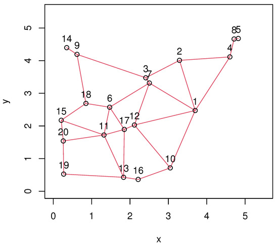
Figure 1. Spatial sampling set $S_{20}$.

For all 20 AUs, spatially weighted estimates of Gaussian distribution parameters and transition probabilities are presented in Table 2.

Table 2. Spatially weighted estimators of the HMM parameters for 20 AUs $IR=0.7$.

i	${\left({\tilde{\mathit{\beta }}}_0^{(\mathit{i})}\right)}^{\prime }$	${\left({\tilde{\mathit{\beta }}}_1^{(\mathit{i})}\right)}^{\prime }$	${\tilde{\mathit{\sigma }}}_{\mathit{i}}^2$	${\tilde{\mathit{a}}}_{{\mathit{y}}_{\mathit{T}}^{(\mathit{i})},0}^{(\mathit{i})}:\mathit{M}1$	${\tilde{\mathit{a}}}_{{\mathit{y}}_{\mathit{T}}^{(\mathit{i})},0}^{(\mathit{i})}:\mathit{M}2$	${\tilde{\mathit{a}}}_{{\mathit{y}}_{\mathit{T}}^{(\mathit{i})},1}^{(\mathit{i})}:\mathit{M}1$	${\tilde{\mathit{a}}}_{{\mathit{y}}_{\mathit{T}}^{(\mathit{i})},1}^{(\mathit{i})}:\mathit{M}2$
1	−0.043, −0.133, −0.126	0.043, 0.133, 0.126	0.249	0.361	0.561	0.341	0.439
2	−0.035, −0.095, −0.128	0.044, 0.125, 0.164	0.323	0.167	0.684	0.200	0.316
3	−0.040, −0.103, −0.141	0.044, 0.117, 0.157	0.317	0.806	0.342	0.777	0.658
4	−0.015, −0.069, −0.065	0.044, 0.206, 0.194	0.320	0.369	0.663	0.241	0.337
5	−0.015, −0.069, −0.068	0.043, 0.205, 0.201	0.314	0.329	0.663	0.233	0.337
6	−0.099, −0.114, −0.262	0.008, 0.013, 0.021	0.318	0.665	0.469	0.635	0.531
7	−0.044, −0.122, −0.140	0.044, 0.121, 0.138	0.280	0.708	0.403	0.706	0.597
8	−0.015, −0.069, −0.066	0.044, 0.206, 0.197	0.317	0.651	0.337	0.763	0.663
9	−0.049, −0.024, −0.211	0.024, 0.012, 0.101	0.316	0.751	0.429	0.699	0.571
10	−0.142 −0.351, −0.067	−0.028, −0.061, −0.010	0.261	0.646	0.459	0.639	0.541
11	−0.165, −0.256, −0.296	−0.013, −0.014, −0.021	0.279	0.413	0.602	0.298	0.398
12	−0.119, −0.233, −0.232	0.015, 0.031, 0.030	0.331	0.672	0.429	0.692	0.571
13	−0.201, −0.405, −0.080	−0.092, −0.180, −0.037	0.324	0.726	0.480	0.633	0.520
14	−0.049, −0.024, −0.211	0.024, 0.012, 0.101	0.316	0.751	0.429	0.699	0.571
15	−0.263, −0.064, −0.466	−0.132, −0.033, −0.223	0.263	0.523	0.327	0.767	0.674
16	−0.171, −0.378, −0.073	−0.060, −0.120, −0.024	0.293	0.314	0.531	0.364	0.469
17	−0.142, −0.244, −0.264	0.001, 0.008, 0.005	0.305	0.630	0.413	0.697	0.587
18	−0.099, −0.114, −0.262	0.008, 0.013, 0.021	0.318	0.665	0.469	0.635	0.531
19	−0.561, −0.150, −0.466	−0.464, −0.125, −0.348	0.338	0.400	0.653	0.252	0.347
20	−0.412, −0.107, −0.466	−0.298, −0.079, −0.285	0.301	0.562	0.337	0.758	0.663

Conditional distribution of $Y_{T+1}^{(i)}$ given $Y_T^{(i)}=1$ is Bernoully with parameter ${\widehat{a}}_{11}^{(i)}$, i.e., $(Y_{T+1}^{(i)}|Y_T^{(i)}=1)\sim Be({\widehat{a}}_{11}^{(i)})$. Hence, it is obvious that $(Y_{T+1}^{(i)}|Y_T^{(i)}=0)\sim Be({\widehat{a}}_{00}^{(i)})$.

At first, we generate $m=100$ simulation runs (replications) for test label by the Bernoulli distribution described above and corresponding conditional Gaussian observation.

Furthermore, we compute performance measures ACC and BAC for each AUs and present their spatially averaged values in Table 3.

Table 3. Averaged performance of classifiers based on PBDF for simulated data.

IR		PSW1	CSW1	PSW2	CSW2
0.1	ACC	0.8395	0.8850	0.5480	0.6125
	BAC	0.8864	0.9241	0.6778	0.7075
0.3	ACC	0.8660	0.8875	0.8100	0.8235
	BAC	0.8647	0.8823	0.8300	0.8450
0.4	ACC	0.7395	0.7525	0.7365	0.7455
	BAC	0.7421	0.7568	0.7413	0.7519
0.5	ACC	0.8790	0.9240	0.8770	0.9220
	BAC	0.8853	0.9278	0.8831	0.9261
0.6	ACC	0.7825	0.7945	0.8035	0.8260
	BAC	0.7879	0.7938	0.8114	0.8283
0.7	ACC	0.9150	0.9175	0.9215	0.9255
	BAC	0.9053	0.9095	0.9066	0.9137
0.9	ACC	0.8610	0.8585	0.9625	0.9655
	BAC	0.7878	0.7864	0.8777	0.8891

As we can see from Table 3, classifiers based on HMM with CSW level of spatial weighting in majority cases have an advantage over one with PSW level of spatial weighting by ACC as well as BAC performance measures for various $IR$ values.

Estimation method M1 has advantage against M2 for smaller values of $IR=0.1,0.3,0.4$. However, M2 ensures greater classification accuracy for $IR=0.6,0.7,0.9$.

5. Real Data Example

The numerical analysis of annual death rate data collected by the Institute of Hygiene of the Republic of Lithuania from the 60 municipalities in the period from 2001 to 2019 is carried out.

Crude death rate for each municipality measured in units per one hundred thousand population is considered as variable Z. We consider two label variables: one is specified by the threshold mortality index due to acute cardiovascular event (ACE) and other is specified by the threshold mortality index due to diseases of the circulatory system (CSD).

Cases with index values less than threshold have label value equal 0 and have label value equal 1. Here, we consider the case with constant mean, i.e., ${\mu }_l(s;t)={\beta }_l$, with $x(s)=1$.

Then, for $i=1,\dots ,60$

$$\begin{array}{c}\hfill X^{(i)}=\left(\begin{array}{cc}1-y_1^{(i)}& y_1^{(i)}\\ 1-y_2^{(i)}& y_2^{(i)}\\ ⋮& ⋮\\ 1-y_T^{(i)}& y_T^{(i)}\end{array}\right).\end{array}$$

Numerical illustrations are performed on 60 areas in two dimensional areas that are depicted in Figure 2.

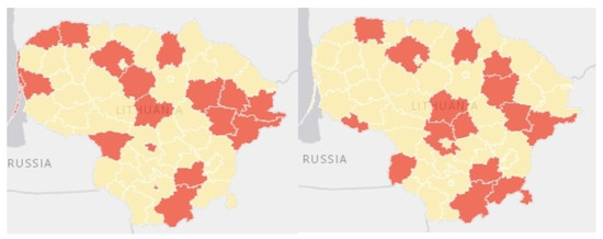
Figure 2. Classified Lithuanian municipalities in 2018 (left) and 2019 (right). Yellow color areas indicate municipalities with low level of mortality due to ACE (with label value 0) and red areas indicates municipalities with high level of mortality due to ACE (with label value 1).

Data in the period from 2001 to 2018 ($t=1,\dots ,18$) are used for training and remaining data (period 2019) are used for testing. Hence, $T=18$ and $n=60$, i.e., we consider $18\times 60$ observations for training and 60 for testing. Here, $IR$ values are calculated for testing data by changing the thresholds in specification of the mortality levels.

The values of performance measures for the proposed classifiers specified in Equations (6) and (7) are presented in Table 4.

Table 4. Performance measures of classifiers based on PBDF for real data.

	$\mathit{IR}$		PSW1	CSW1	PSW2	CSW2
ACE	0.2	ACC	0.7167	0.8333	0.9167	0.9500
		BAC	0.8559	0.9153	0.9576	0.9746
	0.3	ACC	0.6667	0.7833	0.8000	0.8667
		BAC	0.8246	0.8860	0.8947	0.7719
	0.4	ACC	0.6000	0.6833	0.7500	0.8333
		BAC	0.6296	0.6759	0.7130	0.6852
	0.5	ACC	0.6333	0.6500	0.7500	0.8333
		BAC	0.6471	0.5654	0.6699	0.7190
CSD	0.2	ACC	0.6500	0.8167	0.7833	0.8500
		BAC	0.5804	0.6696	0.6518	0.6875
	0.3	ACC	0.7500	0.8167	0.8167	0.8167
		BAC	0.7500	0.7857	0.6696	0.6696
	0.4	ACC	0.6667	0.7833	0.8000	0.7667
		BAC	0.6979	0.8021	0.7813	0.7604
	0.5	ACC	0.6000	0.6167	0.7500	0.7000
		BAC	0.6125	0.6375	0.7500	0.7000

As it might be seen from Table 4, classifiers based on HMM with CSW level of spatial weighting in majority cases have an advantage over one with PSW level of spatial weighting by ACC as well BAC performance measures for various $IR$ values. The similar trend is detected for CSD disease case. Exceptions to this rule is depicted in the table by bold figures.

ROC plot of is presented in Figure 3 visualizes the classifier performances with $IR=0.2$ induced by different classifiers. Depicted points represent four considered classifiers and a random classifier. It is easy to check that the area under the curve in the ROC plot is equal the performance measure BAC.

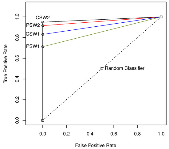
Figure 3. ROC plots for the problems with class label variables ACE with $IR=0.2$.

As can be seen from Figure 3, the classifier CSW2 shows advantage against others since has the largest area under the curve that is equal to 0.95 (see in Table 4).

6. Conclusions

In this paper, we developed the novel supervised generative approach to Bayesian classification of areal Gaussian data based on HMM implementing spatial weighting in several levels. A real data study has been conducted, and critical comparison of the performance of the classifiers with decision threshold values induced by different spatial autocorrelation indexes are performed.

The proposed methodology has several attractive features that make it compare favorably against other approaches to generative supervised spatial classification based on HMM.

First, the method is applicable to HMM with discrete and continuous observation on regular and irregular areal units.

Second, the approach provides an easily interpretable methods of spatial weighting for the local HMM parameters.

Third, proposed classification methodology can be easily specified in terms of undirected and directed graphs.

The obtained results with simulated and real data showed that the spatial weighting level significantly influenced the performance of proposed classifiers.

Based on the calculation results, the suggestions for the selection of transition probabilities estimation method is presented.

It should be also noted that derived closed form PCC could be essentially used in specifying theoretical values of model parameters.

There are several reasons for further research. First, there is further scope for exploring techniques supervising classification due to HMM of spatiotemporal Gaussian data to multiclass case. Second, future research may also include implementation of the proposed classification technique in the context of other continuous non-Gaussian models of observations. Third, in future research, it is reasonable to consider second-order Markov chain model for labels instead of first-order Markov chain. That will enable us to incorporate more information on stochastic temporal dependence.

Presented critical comparison of the performances of classifiers with different level of incorporated spatial information and types of parameter estimators can aid in the selection of proper classification rules of spatiotemporal areal data specified by HMM with Gaussian or other continuous observations.

References

- Ng, A.Y.; Jordan, M.I. On Discriminative vs. Generative Classifiers: A comparison of logistic regression and naive Bayes. NIPS Neural Inf. Process. Syst. 2001, 14, 33. [Google Scholar]
- Zuanetti, D.A.; Milan, L.A. Second-order autoregressive Hidden Markov Model. Braz. J. Probab. Stat. 2017, 31, 653–665. [Google Scholar] [CrossRef]
- Bryan, J.D.; Levinson, S.E. Autoregressive Hidden Markov Model and the Speech Signal. Procedia Comput. Sci. 2015, 61, 328–333. [Google Scholar] [CrossRef]
- Nguyen, L. Continuous Observation Hidden Markov Model. Rev. Kasmera 2016, 44, 65–149. [Google Scholar]
- Gong, W.; Fang, S.; Yang, G.; Ge, M. Using a Hidden Markov Model for Improving the Spatial-Temporal Consistency of Time Series Land Cover Classification. Int. J. Geo-Inf. 2017, 6, 292. [Google Scholar] [CrossRef]
- Shekhar, S.; Schrater, P.R.; Vatsavai, R.R.; Wu, W.; Chawla, S. Spatial contextual classification and prediction models for mining geospatial data. IEEE Trans. Multimed. 2002, 4, 174–188. [Google Scholar]
- Atkinson, P.M.; Lewis, P. Geostatistical classification for remote sensing: An introduction. Comput. Geosci. 2000, 26, 361–371. [Google Scholar] [CrossRef]
- Tang, Y.; Jing, L.; Li, H.; Atkinson, P.M. A multiple-point spatially weighted k-NN method for object-based classification. Int. J. Appl. Earth Obs. Geoinf. 2016, 52, 263–274. [Google Scholar] [CrossRef]
- Kadhem, S.K.; Hewson, P.; Kaimi, I. Using hidden Markov models to model spatial dependence in a network. Aust. N. Z. J. Stat. 2018, 60, 423–446. [Google Scholar] [CrossRef]
- Hamdi, A.; Shaban, K.; Erradi, A.; Mohamed, A.; Rumi, S.K.; Salim, F.D. Spatiotemporal data mining: A survey on challenges and open problems. Artif. Intell. Rev. 2022, 55, 1441–1488. [Google Scholar] [CrossRef]
- Mishra, B.; Dahal, A.; LuinteL, N.; Shahi, T.B.; Panthi, S.; Pariyar, S.; Ghimire, B.R. Methods in the spatial deep learning: Current status and future direction. Spat. Inf. Res. 2022, 30, 215–232. [Google Scholar] [CrossRef]
- Demel, S.S.; Du, J. Spatio-temporal models for some data sets in continuous space and discrete time. Stat. Sin. 2015, 25, 81–98. [Google Scholar]
- Haslett, J.; Raftery, A.E. Space-Time Modelling with Long Memory Dependence: Assessing Ireland’s Wind Power Resource. Appl. Stat. 1989, 38, 1–50. [Google Scholar] [CrossRef]
- Blangiardo, M.; Cameletti, M. Spatial and Spatio-Temporal Bayesian Models with R-INLA; Wiley, John Wiley & Sons: Hoboken, NJ, USA, 2015; pp. 235–258. [Google Scholar]
- Blangiardo, M.; Cameletti, M.; Baio, G.; Rue, H. Spatial and spatio-temporal models with R-INLA. Spat. Spatio-Temporal Epidemiol. 2013, 7, 39–55. [Google Scholar] [CrossRef] [PubMed]
- Cressie, N.; Wikle, C.K. Statistics for Spatio-Temporal Data; Wiley: Hoboken, NJ, USA, 2011. [Google Scholar]
- Fontanella, L.; Ippoliti, L.; Martin, R.J.S. Trivisonno. Interpolation of spatial and spatio-temporal Gaussian fields using Gaussian Markov random fields. Adv. Data Anal. Classif. 2008, 2, 63–79. [Google Scholar] [CrossRef]
- Giannotti, F.; Pedreschi, D. Mobility, Data Mining and Privacy: Geographic Knowledge Discovery; Springer: Berlin/Heidelberg, Germany, 2008. [Google Scholar]
- Berrett, C.; Calder, C.A. Bayesian spatial binary classification. Spat. Stat. 2016, 16, 72–102. [Google Scholar] [CrossRef]
- Dučinskas, K. Approximation of the expected error rate in classification of the Gaussian random field observations. Stat. Probab. Lett. 2009, 79, 138–144. [Google Scholar] [CrossRef]
- Murphy, K.P. Machine Learning: A Probabilistic Perspective; MIT Press: Cambridge, MA, USA, 2012. [Google Scholar]
- Sensoy, M.; Kaplan, L.; Cerutti, F.; Saleki, M. Uncertainty-Aware Deep Classifiers Using Generative Models. Proc. Aaai Conf. Artif. Intell. 2020, 34, 5620–5627. [Google Scholar] [CrossRef]
- Dreižienė, L.; Dučinskas, K. Comparison of spatial linear mixed models for ecological data based on the correct classification rates. Spat. Stat. 2020, 35, 100395. [Google Scholar] [CrossRef]
- Dučinskas, K.; Dreižienė, L. Risks of Classification of the Gaussian Markov Random Field Observations. J. Classif. 2018, 35, 422–436. [Google Scholar] [CrossRef]
- Dučinskas, K.; Dreižienė, L. Performance Evaluations of Gaussian Spatial Data Classifiers Based on Hybrid Actual Error Rate Estimators. Aust. J. Stat. 2020, 49, 27–34. [Google Scholar] [CrossRef]
- Karaliutė, M.; Dučinskas, K. Classification of Gaussian spatio-temporal data with stationary separable covariances. Nonlinear Anal. Model. Control 2021, 26, 363–374. [Google Scholar] [CrossRef]
- Karaliutė, M.; Dučinskas, K. Supervised linear classification of Gaussian spatio-temporal data. Liet. Mat. Rinkinys. Proc. Lith. Math. Soc. 2021, 62, 9–15. [Google Scholar] [CrossRef]
- McLachlan, G.J. Discriminant Analysis and Statistical Pattern Recognition; Wiley: New York, NY, USA, 2004. [Google Scholar]
- Diggle, P.J.; Ribeiko, P.J.; Christensen, O.F. An introduction to model-based geostatistics. Spat. Stat. Comput. Methods Lect. Notes Stat. 2003, 173, 43–86. [Google Scholar]
- Zhu, Z.; Stein, M.L. Spatial sampling design for prediction with estimated parameters. J. Agric. Biol. Environ. Stat. 2006, 11, 24–44. [Google Scholar] [CrossRef]
- López, V.; Fernández, A.; García, S.; Palade, V. Herrera, F. An insight into classification with imbalanced data: Empirical results and current trends on using data intrinsic characteristics. Inf. Sci. 2013, 250, 113–141. [Google Scholar] [CrossRef]
- Orriols-Puig, A.E. Bernadó-Mansilla, Evolutionary rule-based systems for imbalanced datasets. Soft Comput. 2009, 13, 213–225. [Google Scholar] [CrossRef]
- Ortigosa-Hernández, J.; Inza, I.; Lozano, J.A. Measuring the class-imbalance extent of multi-class problems. Pattern Recognit. Lett. 2017, 98, 32–38. [Google Scholar] [CrossRef]
- Soleymani, R.; Granger, E.; Fumera, G. F-measure curves: A tool to visualize classifier performance under imbalance. Pattern Recognit. 2020, 100, 107146. [Google Scholar] [CrossRef]
- Scaccia, L.; Martin, R.J. Testing axial symmetry and separability of lattice processes. J. Stat. Plan. Inference 2005, 131, 19–39. [Google Scholar] [CrossRef]
Disclaimer/Publisher’s Note: The statements, opinions and data contained in all publications are solely those of the individual author(s) and contributor(s) and not of MDPI and/or the editor(s). MDPI and/or the editor(s) disclaim responsibility for any injury to people or property resulting from any ideas, methods, instructions or products referred to in the content. |
© 2023 by the authors. Licensee MDPI, Basel, Switzerland. This article is an open access article distributed under the terms and conditions of the Creative Commons Attribution (CC BY) license (https://creativecommons.org/licenses/by/4.0/).