Abstract
The classical economic growing quantity (EGQ) model is a key concept in the inventory control problems research literature. The EGQ model is commonly employed for the purpose of inventory control in the management of growing items, such as fish and farm animals, within industries such as livestock, seafood, and aviculture. The economic order quantity (EOQ) model assumes that customer demand is satisfied without interruption in each cycle; however, this assumption is not always true for some companies as they do not have continuous operations, except for item storage, during non-working times such as weekends, natural idle periods, or spare time. In this study, we extend the traditional EGQ model by incorporating the concept of working and non-working periods, resulting in the development of a new model called discontinuous economic growing quantity (DEGQ). Unlike the conventional EGQ model, the DEGQ model considers the presence of intermittent operational periods, in which the firm is actively engaged in its activities, and non-working periods, during which only storage-related operations occur. By incorporating this discontinuity, the DEGQ model provides a more accurate representation of real-world scenarios where businesses operate in a non-continuous manner, thus enhancing the effectiveness of inventory control and management strategies. The study aims to obtain the optimal number of periods in each cycle and the optimal slaughter age for the breeding items, and, subsequently, to find the optimal order size to minimize the total cost. Finally, we propose an optimal analytical procedure to determine the optimal solutions. This procedure entails finding the optimal number of periods using a closed-form equation and determining the optimal slaughter age by exhaustively searching the entire range of possible growth times.
Keywords:
economic order quantity (EOQ); economic growing quantity (EGQ); discontinuous periods; idle time; discontinuous economic growing quantity (DEGQ) MSC:
90B05
1. Introduction
The efficient administration of inventory in an organization is one of the key factors in its growth, as well as in ensuring customer satisfaction in an increasingly competitive market. The optimization of inventory contributes to the joint administration of the financial and productive factors in the company, which supports the reduction of costs and consequently increases profits. This effect has motivated researchers to move from traditional inventory control models to new models that reflect special conditions and are more descriptive of the real problems that companies face, such as deficient and decaying items.
The oldest and most well-known traditional inventory model, widely used by researchers, is the economic order quantity (EOQ) model. This model assumes that items experience no physical changes during their consumption periods, although there are products in various industries that cannot be represented by this condition as they undergo some change over time. Changes such as decay, loss of freshness, and/or growth are commonly presented in some products. Hence, Rezaei [1] introduced a modified version of the classical economic order quantity (EOQ) model, known as the economic growing quantity (EGQ) model. He proposed the EGQ model for items that increase in weight after their acquisition and/or during their growth periods, such as farm animals and fishes. The increase in weight during the growth period is the difference between conventional and growing items.
Two different periods are used for growing items in inventory systems: growing and consuming. As soon as the live newborns reach the feeding place, the growth period starts with a known growth function. After the items obtain the defined weight, they are sent for slaughter and the consumption period starts immediately after the items are sent to the warehouse. When this process has ended, the next cycle starts as stated before.
All the inventory studies of growing items assume that the system meets the customer requirement from the beginning to the end of the cycle without interruption. However, this assumption is not always true for some companies as they do not have continuous operations, except for item storage, during non-working times such as weekends, natural idle periods, or spare time. In addition, some stores or distributors are not open during the weekends; therefore, in some situations, the system only sends items to the market on regular workdays. This study extends the classic EGQ model by considering working and non-working periods and offers a model with discontinuous periods, entitled discontinuous economic growing quantity (DEGQ). The system has no activity during non-working times, except for storage; therefore, the system cannot meet the customers’ demand during non-working periods. All items are sent to the market during working periods, to have them available to customers.
The rest of the current study proceeds as follows. Section 2 presents a literature review regarding growing problems and some existing gaps. Section 3 states the formulation of the proposed model. The solution procedure and a numerical example are explained in Section 4. Finally, Section 5 provides some conclusions and future research tracks.
2. Literature Review
Cost optimization in managing an organization’s inventories has been the subject of scientific analysis for more than a century. Nobil et al. [2] mentioned that Harris in 1913 proposed the economic order quantity model, which was the first model in the classic inventory management field. His model focuses on optimizing the cost of ordering and holding in the inventory system. Items are ordered from a supplier in a predetermined lot size; after being received, the system stores the products to fill the demand at a fixed rate of consumption. When the inventory reaches zero, the cycle repeats. As cited by Ruidas et al. [3] and Ruidas et al. [4], after the initial work of Harris, the EOQ model was extended and widely applied in various industries, such as electronic products, fashion items, and spare parts. These extensions and adaptations of the EOQ model have facilitated effective inventory management and optimization strategies in a diverse range of industrial sectors.
In Harris’s model, the volume of items is stable after the purchase, but, in some industries, such as aviculture, livestock, and seafood, items grow after purchase, so their volume increases over time. As a result, the analysis of growing item inventories is an interesting subject for researchers that was introduced by Rezaei [1]. In his study, he formulated a classic EOQ model for a growing item by considering a growth function as follows:
where is the item weight at time ; is the shape parameter; is the integration constant; is the asymptotic weight as the age approaches infinity; and is the growth rate.
After this study, the second paper in this field was presented by Zhang et al. [5]. They supposed that customers prefer to consume products that have the least carbon emissions during their production. Then, Nobil et al. [6] developed the third model of inventory control for growing items, which allows shortages during the system cycle. They used the growing function proposed by Rezaei [1] with a linear approximation.
As a follow-up to these studies, researchers have continued with the analysis of growing item inventory models. Malekitabar et al. [7] presented a two-level supply chain regarding revenue sharing among actors. The model integrates a supplier and a farmer for growing mortal items. Sebatjane and Adetunji [8] and Sebatjane and Adetunji [9] developed a growing EOQ model for a three-echelon supply chain. The models consider sending a certain number of equally sized batches to retailers. Hidayat et al. [10] and Sitanggang et al. [11] integrated incremental discount policies for the acquisition of growing items from a supplier. Sebatjane and Adetunji [12] developed a growing inventory model where some of the growing items have poor quality and a lower selling price after a 100% screening process.
Most studies in the field of growing items include only one type of product, except for Khalilpourazari and Pasandideh’s [13] study, which proposes a growing EOQ model with multiple items. They solve this problem in large size instances through an exact approach, named sequential quadratic programming (SQP), and use two metaheuristic algorithms in large and medium size instances: the sine cosine crow search algorithm and water cycle moth flaws optimization algorithm.
Sebatjane and Adetunji [8] included the effects of freshness and the level of inventory extended in the demand behavior. From a similar perspective, Pourmohammad-Zia et al. [14], De-la-Cruz-Márquez et al. [15], and De-la-Cruz-Márquez et al. [16] supposed that the demand depends on the item’s price, while Rana et al. [17] assumed that the demand is a linear function of time.
Gharaei and Almehdawe [18] calculated the reorder point for the inventory model of growing items. They assumed that the demand is constant, and the objective function is to minimize the system’s total cost. Pourmohammad-Zia et al. [19] and Choudhury and Mahanta [20] investigated the negative effects of overbreeding on growing inventory models. Moreover, Rana et al. [17] considered permissible delay payments when purchasing growing items from a supplier.
Additionally, there are some papers in the lot sizing problem literature that investigate the effects of holidays, weekends, leisure, and/or natural idle periods in the inventory problem. De [21] developed a traditional EOQ model including idle time and the false consumption rate. This study assumes that the firm is open on some days and closed on others during the time horizon and considers that unsatisfied requirements during idle times are added to the total system cost as idle time costs. Afterwards, Das et al. [22] extended the research of De [21] by presenting an inventory model with idle times and full backlogging. Both studies assume that products do not spoil over time. Meanwhile, Karmakar et al. [23] investigated the effects of item deterioration based on the model presented by De [21].
Recently, Nobil et al. [24] presented a novel EOQ model for growing items, specifically focusing on a sustainable green breeding policy. Their model incorporated a mortality function and considered the practical polynomial relationship between carbon dioxide production and the age of the animals, alongside the impact of the mortality function. The primary objective of their model was to identify the optimal slaughter age and the optimal quantity of newborn chicks to be procured from the supplier, with the goal of minimizing the overall costs. Khan et al. [25] investigated the interdependent decisions of joint prepayment installment, pricing, and replenishment for a growing item within the context of different regulatory frameworks: cap-and-price, cap-and-trade, and carbon tax regulations. Their main objective was to maximize the profitability of a livestock farming company while simultaneously reducing the overall carbon emissions associated with its operations. In the same year, Nobil et al. [26] introduced a comprehensive model for economic growth. One key aspect of their model is the inclusion of the cost associated with inhibiting ammonia production during the growing period. Moreover, their model adopted an all-units discount policy, meaning that the price of newly acquired items was determined by the quantity ordered from the supplier. Furthermore, they considered the possibility of certain newborn items being nonviable upon arrival due to stressful experiences and incidents encountered during catching, loading, transportation, and unloading.
In the studies carried out in the field of growing items, researchers have not modeled idle periods for the distribution of the products. On the other hand, the studies developed in the field of inventory management that consider idle time assume that the length of the closing period is a decision variable, and, consequently, the firm can determine it such that the total cost is minimized. However, this assumption is not necessarily practical or feasible, since these idle times are predefined; if the company wishes to change them, it must incur extra costs, such as overtime for working on weekends or holidays. Table 1 provides a summary of the most significant contributions made by scholars in current studies. This study presents an economic growing quantity model for discontinuous periods. It is assumed that the opening (e.g., regular days) and closing (e.g., weekends) times are repeated during the per unit time, and the lengths of both times are known and fixed and the firm cannot change them. The model seeks to determine the optimal number of periods in each cycle and the optimal length of the growing period to minimize the system’s total cost.

Table 1.
A summary of the most notable contributions made by scholars in the field of EGQ.
3. Mathematical Model
The model considers that the firm purchases some newborn animals () with an initial weight from the supplier and breeds them until they reach a desired weight () or slaughter age (). Then, the firm distributes the consumable products to the market only during the working time, e.g., Monday to Friday. Hence, a period () consists of two time intervals: working time () and non-working time (). Mathematically speaking, . An inventory system cycle () consists of periods, . As is known, the breeding process is performed during all periods, both working and non-working times, while product distribution is carried out exclusively during working times, as distribution companies, stores, and retailers only operate on these days. Therefore, the demand, including working and non-working times, is only covered on working days; thus, the working time consumption rate is adapted based on the working and non-working time requirements for all periods. Accordingly, the consumption rate per unit time () is modified as , where is a correction coefficient. Figure 1 illustrates the inventory system for growing items with discontinuous periods. In addition, the rest of the model notation is as follows.
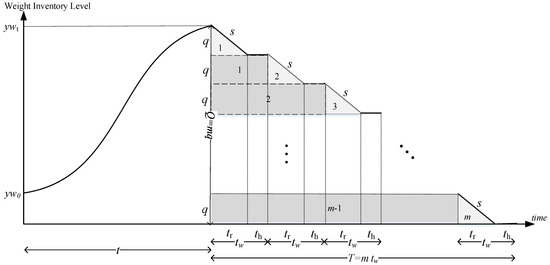
Figure 1.
The behavior of the inventory level of the DEGQ problem.
- Parameters
- : the weight of unit item at time t;
- : the length of working time;
- : the length of non-working time;
- : the length of a period; ;
- : the consumption rate per unit time;
- : the modified consumption rate per unit time based on the length of working time in a unit of time; ;
- : the quantity of the items consumed in each working time period; ;
- : the setup cost per cycle;
- : the purchasing cost per unit of weight;
- : the feeding cost per unit of weight per unit of time;
- : the weight unit holding cost per unit of time;
- : the asymptotic weight;
- : the growth rate;
- : the shape parameter of the growth function;
- : the integration constant of growth;
- : the feeding (production) function.
- Dependent variables
- : the total order quantity per cycle; ;
- : the number of ordered newborn items;
- : the cycle length;
- : the total cost per unit of time.
- Integer decision variables
- : the number of periods in each cycle;
- : the slaughter age (time).
As seen in Figure 1, the quantity of items consumed during each period () is equal to , and, thus, the total quantity of items per cycle is . Hence, the total weight at the slaughter time is calculated by
Based on Equation (1), , and , and the number of ordered newborn items is as follows:
The firm wants to determine the optimal number of periods to be covered with each order and the optimal slaughter time to minimize the total cost, which includes the purchasing cost, the setup cost, the holding cost, and the feeding cost. The purchasing cost per unit of weight is equal to , so the total purchasing cost per cycle is equal to , and the setup cost in each cycle is . Rezaei [1] mentioned that the feeding function is a polynomial function of the form , which relates feed consumption to the item’s age. Consequently, the feeding (production) cost per cycle is equal to . Now, the holding cost is calculated based on the area of the inventory of each cycle, as shown in Figure 1. The area includes triangles and rectangle and is computed as . Given , the holding cost per cycle is . Finally, the total cost per cycle (TCP) is defined as
The total cost per unit time is calculated as follows:
Substituting from Equation (3) into Equation (5), TC is expressed as
4. Solution Procedure and Numerical Example
As is presented in Equation (6), the objective function contains two independent decision variables, and it can be rewritten as follows:
where
Furthermore, it is important to note that the third term of Equation (7) remains constant throughout the optimization process since it does not involve any decision variables.
Equation (8) is a convex function as its second derivation with respect to is always positive; . Therefore, using the derivation method, the optimal number of periods in each cycle () is
However, the value of must be an integer, since each cycle cannot contain fractional periods. In order to obtain an integer solution, the method presented by García-Laguna et al. [28] is applied as follows:
where is .
As shown in Rezaei’s [1] study, demonstrating the convexity of the objective function is a challenging task because of existing growth and feeding curves. Therefore, the convexity of Equation (9) is a challenge. However, within the context of industrial agriculture scenarios, Nobil et al. [24] and Nobil et al. [26] mentioned that slaughter plants kill animals in a limited predetermined age range. However, the European Food Safety Authority [29] states that there exists a disparity between the United States and European countries in terms of typical slaughter ages, with the former commonly observing a slaughter age of 47 days, while the latter adheres to a slaughter age of 42 days. Moreover, Park et al. [30] mentioned that the slaughter age should be at least 30 days. Therefore, in our research, we consider a constrained slaughter age range of 30 to 100 days. As a result, the solution space for the slaughter age, denoted by t, encompasses a total of 71 critical points. To effectively explore these points, we undertake an investigation of the values of Equation (9) for each individual point. By subsequently identifying the point with the lowest value, we determine the optimal solution for Equation (9). In conclusion, we compute the values of with respect to the values of t within the interval of 30 to 100 days, and if a particular point exhibits the lowest value, it is considered the optimal solution for Equation (9).
As mentioned above, the solution procedure for determining the best solution is as follows:
- (1)
- Determine the optimal value of using Equation (11) and then calculate the optimal value of using Equation (8);
- (2)
- Calculate the values of using Equation (9) with respect to the values of t within the interval of 30 to 100 days;
- (3)
- The point with the lowest value of is the optimal slaughter age (;
- (4)
- Based on the optimal values of and , calculate the optimal value of the total cost () using Equation (7).
Numerical Example
To demonstrate the solution procedure outlined in the previous section, two specific instances are presented. These instances serve as examples to illustrate the methodology. In accordance with Rezaei [1], the parameter values for the growth curve and feeding function are defined as follows: g, , , , , , , , and . These values are used in both examples.
- −
- Example 1
We assume a regular week as a period that includes 5 working days and 2 non-working days; then, the working and non-working times in a year are 5/365 = 0.0137 and 2/365 = 0.0055, respectively. Consequently, the period length is equal to 0.0192. Moreover, the consumption rate per year of the first example is g; subsequently, the modified consumption rate per year is equal to g; . The inventory cost data are $/cycle, $/g/day, $/g, and $/year.
Given the stated data and Equation (11), the optimal number () is 48. Based on this optimal number, the optimal value of would be $5531.6 using Equation (7), while the optimal slaughter age is computed as by searching the whole feasible space in the range of 30 to 100 days. Then, the optimal value of is $17,015.4. The plot of as a function of t for the first example is illustrated in Figure 2. Finally, the total cost per year is equal to $22,514. The optimal solution means that the firm consumes g in each period; subsequently, the optimal total weight for each cycle is g. Therefore, the firm orders newborn items, equivalent to g, at the start of every cycle.
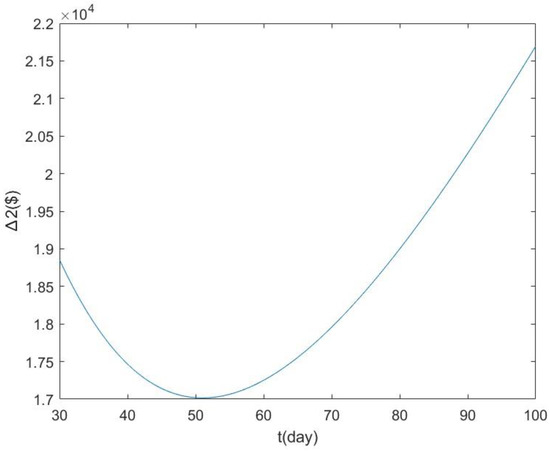
Figure 2.
The plot of with respect to the value of t for Example 1.
- −
- Example 2
In the second example, assuming that a standard week consists of 6 working days and 1 non-working day, the yearly working and non-working times are estimated to be 0.0164 and 0.0027, respectively. Consequently, the period length amounts to 0.0191. The annual consumption rate is initially calculated as g. Following modification, the revised consumption rate per year equals 87,348 g, determined by the formula . The inventory cost data are as follows: $/cycle, $/g/day, $/g, and $/year.
Based on the provided data and Equation (11), the optimal quantity () is determined to be 85. Using Equation (7), the corresponding optimal value of is calculated as $487.2. By exploring the feasible range of 30 to 100 days, the optimal slaughter age is found to be 51. Consequently, the optimal value of is $10,624.8. Figure 3 illustrates the plot of as a function of t for this example. Finally, the total cost per year amounts to $11,111. The optimal solution dictates that the company consumes a quantity of g per period, resulting in an optimal total weight of 104,550 g for each cycle. Therefore, the company places orders for newborn items, which is equivalent to g, at the beginning of each cycle.
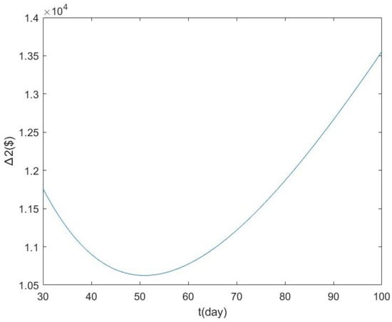
Figure 3.
The plot of with respect to the value of t for Example 2.
5. Conclusions
This study extends the classic economic order quantity model for growing items by considering the real condition including idle times. Some firms, particularly distributors, do not have any operational activities, except for item storage, during holidays or weekends. Hence, the classic EGQ inventory model is not useful for them. It is assumed that each cycle includes working and non-working times; thus, for the first time in this area, a discontinuous economic order quantity for growing items model, entitled DEGQ, is presented. The model seeks to find the optimal number of periods in each cycle and the optimal slaughter age and subsequently obtain the optimal order size that minimizes the system’s total cost. Then, the optimal solutions are computed using a combination of the derivation method for the optimal number of periods () and the Newton–Raphson method for the optimal slaughter age. Finally, the optimal order size and the optimal total cost are calculated based on the optimal values obtained.
The proposed model can be extended (a) by considering the effects of mortality on the breeding process, (b) by introducing shortages during working and/or non-working times, (c) by considering permissible delay payments in the acquisition of the growing items, (d) by breeding multi-items, and (e) by modeling the perishable conditions of the growing items after slaughtering.
Author Contributions
Conceptualization, A.H.N., E.N., L.E.C.-B., D.G.-N., G.T.-G., A.C.-M., I.d.J.L.-H. and N.R.S.; Methodology, A.H.N., E.N., L.E.C.-B., D.G.-N., G.T.-G., A.C.-M., I.d.J.L.-H. and N.R.S.; Software, A.H.N. and L.E.C.-B.; Validation, A.H.N., E.N. and L.E.C.-B.; Formal analysis, A.H.N., E.N., L.E.C.-B., D.G.-N., G.T.-G., A.C.-M., I.d.J.L.-H. and N.R.S.; Investigation, A.H.N., E.N., L.E.C.-B., D.G.-N., G.T.-G., A.C.-M., I.d.J.L.-H. and N.R.S.; Data curation, A.H.N., E.N., L.E.C.-B., D.G.-N., G.T.-G., A.C.-M., I.d.J.L.-H. and N.R.S.; Writing—original draft, A.H.N. and E.N.; Writing—review & editing, L.E.C.-B.; Visualization, A.H.N., E.N. and L.E.C.-B.; Supervision, L.E.C.-B. All authors have read and agreed to the published version of the manuscript.
Funding
The APC was funded by Tecnológico de Monterrey.
Data Availability Statement
Not applicable.
Conflicts of Interest
The authors declare no conflict of interest.
References
- Rezaei, J. Economic order quantity for growing items. Int. J. Prod. Econ. 2014, 155, 109–113. [Google Scholar] [CrossRef]
- Nobil, A.H.; Niaki, S.T.A.; Niaki, S.A.A.; Cárdenas-Barrón, L.E. An economic production quantity inventory model for multi-product imperfect production system with setup time/cost function. Rev. Real Acad. Cienc. Exactas Físicas Nat. Ser. A Mat. 2022, 116, 49. [Google Scholar] [CrossRef]
- Ruidas, S.; Seikh, M.R.; Nayak, P.K.; Sarkar, B. A single period production inventory model in interval environment with price revision. Int. J. Appl. Comput. Math. 2019, 5, 7. [Google Scholar] [CrossRef]
- Ruidas, S.; Seikh, M.R.; Nayak, P.K. A production inventory model for high-tech products involving two production runs and a product variation. J. Ind. Manag. Optim. 2023, 19, 2178–2205. [Google Scholar]
- Zhang, Y.; Li, L.Y.; Tian, X.Q.; Feng, C. Inventory management research for growing items with carbon-constrained. In Proceedings of the 2016 35th Chinese Control Conference (CCC), Chengdu, China, 27–29 July 2016; IEEE: Piscataway, NJ, USA, 2016. [Google Scholar]
- Nobil, A.H.; Sedigh, A.H.A.; Cárdenas-Barrón, L.E. A generalized economic order quantity inventory model with shortage: Case study of a poultry farmer. Arab. J. Sci. Eng. 2019, 44, 2653–2663. [Google Scholar] [CrossRef]
- Malekitabar, M.; Yaghoubi, S.; Gholamian, M.R. A novel mathematical inventory model for growing-mortal items (case study: Rainbow trout). Appl. Math. Model. 2019, 71, 96–117. [Google Scholar] [CrossRef]
- Sebatjane, M.; Adetunji, O. Economic order quantity model for growing items with incremental quantity discounts. J. Ind. Eng. Int. 2019, 15, 545–556. [Google Scholar] [CrossRef]
- Sebatjane, M.; Adetunji, O. Optimal lot-sizing and shipment decisions in a three-echelon supply chain for growing items with inventory level-and expiration date-dependent demand. Appl. Math. Model. 2021, 90, 1204–1225. [Google Scholar] [CrossRef]
- Hidayat, Y.A.; Riaventin, V.N.; Jayadi, O. Economic order quantity model for growing items with incremental quantity discounts, capacitated storage facility, and limited budget. J. Tek. Ind. 2020, 22, 1–10. [Google Scholar] [CrossRef]
- Sitanggang, I.V.; Rosyidi, C.N.; Aisyati, A. The Development of Order Quantity Optimization Model for Growing Item Considering the Imperfect Quality and Incremental Discount in Three Echelon Supply Chain. J. Tek. Ind. 2021, 23, 101–110. [Google Scholar] [CrossRef]
- Sebatjane, M.; Adetunji, O. Three-echelon supply chain inventory model for growing items. J. Model. Manag. 2019, 15, 567–587. [Google Scholar] [CrossRef]
- Khalilpourazari, S.; Pasandideh, S.H.R. Modeling and optimization of multi-item multi-constrained EOQ model for growing items. Knowl. Based Syst. 2019, 164, 150–162. [Google Scholar] [CrossRef]
- Pourmohammad-Zia, N.; Karimi, B.; Rezaei, J. Food supply chain coordination for growing items: A trade-off between market coverage and cost-efficiency. Int. J. Prod. Econ. 2021, 242, 108289. [Google Scholar] [CrossRef]
- De-la-Cruz-Márquez, C.G.; Cárdenas-Barrón, L.E.; Mandal, B. An inventory model for growing items with imperfect quality when the demand is price sensitive under carbon emissions and shortages. Math. Probl. Eng. 2021, 2021, 6649048. [Google Scholar] [CrossRef]
- De-la-Cruz-Márquez, C.G.; Cárdenas-Barrón, L.E.; Mandal, B.; Smith, N.R.; Bourguet-Díaz, R.E.; Loera-Hernández, I.D.J.; Céspedes-Mota, A.; Treviño-Garza, G. An inventory model in a three-echelon supply chain for growing items with imperfect quality, mortality, and shortages under carbon emissions when the demand is price sensitive. Mathematics 2022, 10, 4684. [Google Scholar] [CrossRef]
- Rana, K.; Singh, S.R.; Saxena, N.; Sana, S.S. Growing items inventory model for carbon emission under the permissible delay in payment with partially backlogging. Green Financ. 2021, 3, 153–174. [Google Scholar] [CrossRef]
- Gharaei, A.; Almehdawe, E. Optimal sustainable order quantities for growing items. J. Clean. Prod. 2021, 307, 127216. [Google Scholar] [CrossRef]
- Pourmohammad-Zia, N.; Karimi, B.; Rezaei, J. Dynamic pricing and inventory control policies in a food supply chain of growing and deteriorating items. Ann. Oper. Res. 2021, 304, 1–40. [Google Scholar] [CrossRef]
- Choudhury, M.; Mahata, G.C. RETRACTED: Sustainable integrated and pricing decisions for two-echelon supplier–retailer supply chain of growing items. RAIRO-Oper. Res. 2021, 55, 3171–3195. [Google Scholar] [CrossRef]
- De, S.K. EOQ model with natural idle time and wrongly measured demand rate. Int. J. Inventory Control Manag. 2013, 3, 329–354. [Google Scholar] [CrossRef]
- Das, P.; Kumar De, S.; Sana, S.S. An EOQ model for time dependent backlogging over idle time: A step order fuzzy approach. Int. J. Appl. Comput. Math. 2015, 1, 171–185. [Google Scholar] [CrossRef]
- Karmakar, S.; De, S.K.; Goswami, A. A deteriorating EOQ model for natural idle time and imprecise demand: Hesitant fuzzy approach. Int. J. Syst. Sci. Oper. Logist. 2017, 4, 297–310. [Google Scholar] [CrossRef]
- Nobil, A.H.; Nobil, E.; Cárdenas-Barrón, L.E.; Garza-Núñez, D.; Treviño-Garza, G.; Céspedes-Mota, A.; Loera-Hernández, I.D.J.; Smith, N.R. Economic Growing Quantity Model with Mortality in Newborn Items and Inhibition Cost of Ammonia Production under All-Units Discount Policy. Sustainability 2023, 15, 8086. [Google Scholar] [CrossRef]
- Khan, M.A.A.; Cárdenas-Barrón, L.E.; Treviño-Garza, G.; Céspedes-Mota, A.; De Jesús Loera-Hernández, I. Integrating prepayment installment, pricing and replenishment decisions for growing items with power demand pattern and non-linear holding cost under carbon regulations. Comput. Oper. Res. 2023, 156, 106225. [Google Scholar] [CrossRef]
- Nobil, A.H.; Nobil, E.; Cárdenas-Barrón, L.E.; Garza-Núñez, D.; Treviño-Garza, G.; Céspedes-Mota, A.; Loera-Hernández, I.D.J.; Smith, N.R. Economic Order Quantity for Growing Items with Mortality Function under Sustainable Green Breeding Policy. Mathematics 2023, 11, 1039. [Google Scholar] [CrossRef]
- Nobil, A.; Taleizadeh, A.A. Economic Order Quantity for Growing Items with Discrete Orders. J. Model. Eng. 2019, 17, 123–129. [Google Scholar]
- García-Laguna, J.; San-José, L.A.; Cárdenas-Barrón, L.E.; Sicilia, J. The integrality of the lot size in the basic EOQ and EPQ models: Applications to other production-inventory models. Appl. Math. Comput. 2010, 216, 1660–1672. [Google Scholar] [CrossRef]
- European Food Safety Authority. Technical assistance to the Commission (Article 31 of Regulation (EC) No 178/2002) for the preparation of a data collection system of welfare indicators in EU broilers’ slaughterhouses. Eur. Food Saf. Auth. J. 2013, 11, 3299. [Google Scholar] [CrossRef]
- Park, S.Y.; Byeon, D.S.; Kim, G.W.; Kim, H.Y. Carcass and retail meat cuts quality properties of broiler chicken meat based on the slaughter age. J. Anim. Sci. Technol. 2021, 63, 180. [Google Scholar] [CrossRef] [PubMed]
Disclaimer/Publisher’s Note: The statements, opinions and data contained in all publications are solely those of the individual author(s) and contributor(s) and not of MDPI and/or the editor(s). MDPI and/or the editor(s) disclaim responsibility for any injury to people or property resulting from any ideas, methods, instructions or products referred to in the content. |
© 2023 by the authors. Licensee MDPI, Basel, Switzerland. This article is an open access article distributed under the terms and conditions of the Creative Commons Attribution (CC BY) license (https://creativecommons.org/licenses/by/4.0/).