Asymptotic Expansions for Moench’s Integral Transform of Hydrology

Abstract

Theis’ theory (1935), later improved by Hantush & Jacob (1955) and Moench (1971), is a technique designed to study the water level in aquifers. The key formula in this theory is a certain integral transform $H\left[g\right](r,t)$ of the pumping function g that depends on the time t and the relative position r to the pumping point as well as on other physical parameters. Several analytic approximations of $H\left[g\right](r,t)$ have been investigated in the literature that are valid and accurate in certain regions of r, t and the mentioned physical parameters. In this paper, the analysis of possible analytic approximations of $H\left[g\right](r,t)$ is completed by investigating asymptotic expansions of $H\left[g\right](r,t)$ in a region of the parameters that is of interest in practical situations, but that has not yet been investigated. Explicit and/or recursive algorithms for the computation of the coefficients of the expansions and estimates for the remainders are provided. Some numerical examples based on an actual physical experiment conducted by Layne-Western Company in 1953 illustrate the accuracy of the approximations.

1. Introduction

Pumping from a well, group of wells or any kind of water reserve has been the subject of a deep study by specialized geologists in the last century. One of the most important subjects of investigation in this area is the prediction of the water level in the aquifer due to pumping mechanisms and pumping techniques that have evolved over time due to continuous technological improvements. It would be an impossible mission to cite all the important contributions to this topic, most of which were published in specialized journals of geology. Without the aim of being exhaustive, a few of them that give an idea about the state of the art in the problem of predicting water levels in aquifers due to different pumping mechanisms are mentioned: [1,2,3,4,5,6,7,8,9]. In order to obtain a complete picture of the problem, a review of these references and references therein is suggested.

Until 1971, the mathematical models that describe the water level changes were based on Theis’ theory [8] and the superimposition of the effects of each pumping well [7,9] for both leaky and nonleaky aquifers. The first precise mathematical model was proposed in [4], which is used to predict water level changes at a certain point of an aquifer when a variable pumping is acting from one or more wells. Their main contribution is the derivation of an integral representation of the drawdown of water in the aquifer in the form of a convolution integral, which is valid when the pumping is constant. Their theory is improved and generalized by [6] for an arbitrary pumping. The key formula that gives the response of the aquifer due to an arbitrary pumping is the convolution integral

$$H\left[g\right](r,t):=\frac{1}{4\pi T}{\int }_0^t\frac{g\left(u\right)}{u}\exp \left\{-\frac{S{r}^2}{4T}\frac{1}{u}-\frac{P}{Sm}u\right\}du.$$

(1)

In this formula, $H\left[g\right](r,t)$ represents the drawdown as a function of the distance r to the pumping point and of the time t elapsed since the beginning of the pumping, all of which are measured in natural unities. The parameter S is the (dimensionless) storage coefficient; T is the transmissivity coefficient (measured in units $Lengt{h}^2/Time$); P is the vertical permeability of the confining layer (measured in speed units $Length/Time$); m is the thickness of the confining layer (measured in length units $Length$); and $g\left(t\right)$ is the pumping as a function of time (measured in units $Lengt{h}^3/Time$). The three parameters m, S and T are positive, and P is non-negative. Hantush and Jacob’s formula [1,2] is the particular case of Moench’s Formula (1) when the pumping is constant, $g\left(t\right)=1$. On the other hand, as a difference with Theis’ theory, Formula (1) assumes a negligible storage capacity of the confining layer and that the leakage rate through this layer is proportional to the drawdown in the aquifer. When $P\ne 0$, the aquifer is said leaky, and it is nonleaky when $P=0$.

Formula (1) gives a quite accurate description of the level changes in the aquifer. However, it has some limitations, since there are some physical situations, more or less relevant in practice, that are not taken into account in Moench’s theory. They are described by Moench himself in [6]. One of them is, for example, the presence of boundaries in the aquifer that are not included in the theoretical analysis, although it could be handled by using image theory [6]. For a more detailed description of the limitations of Moench’s theory, see [6].

A partially penetrating pumping well has an effect on the vertical components of the water flow. Thus, in the presence of partially penetration effects in a leaky confined aquifer, some terms must be added on the right-hand side of (1) [10,11]: terms that are a combination of elementary functions as well as Bessel functions. Other variations and alternative representations in terms of Bessel functions may be found in [5]. In the case of the presence of parallel unsteady-state flow, Vanderberg showed that the denominator in Formula (1) must be slightly modified $u\to u^{3/2}$ or, in other words, that a constant pumping translates into $g\left(t\right)=t^{-1/2}$ [12,13].

Therefore, from a mathematical point of view, the following integral transform of a function g for which the integral exists is of interest,

$$S_t\left[g\right](x,y):={\int }_0^{t}g\left(u\right)\frac{e^{-xu-y/u}}{u}du={\int }_0^{1}g\left(tu\right)\frac{e^{-xtu-y/\left(tu\right)}}{u}du,x\ge 0,y>0,$$

(2)

with $t>0$ or $t=\infty$ (in the case $t=\infty$, only the first integral above is considered). The integral transform considered in Chapter 27 of [14] is the particular case $t=\infty$ of the above formula. Chapter 27 in [14] contains several asymptotic expansions in terms of Bessel functions as well as several illustrative examples. In addition, the particular case $t=\infty$ and $g\left(u\right)=u^p$ is a Krätzel integral, which was introduced in [15]. Apart from a constant factor, integral (1) is integral (2) with the identification $x=P/\left(2m\right)$ and $y=S{r}^2/\left(4T\right)$. Therefore, integral (2) is from now on called Moench’s transform of the function g.

Even for elementary pumping functions $g\left(t\right)$, the right-hand side of (2) cannot be evaluated in terms of elementary functions. Many numerical techniques have been considered in the literature for the evaluation of the right-hand side of (2) and eventually implemented in computer codes and compared with experimental data obtained from several aquifer systems (see for example [2,6,9]). In this paper, analytic approximations of (2) are of interest. Several analytic approximations, convergent or asymptotic, have been proposed in the literature in several limits of the parameters x, y and t. According to the experiments described in [1,2,3,4,5,6,7,8,9] and from a practical point of view, it is of interest to evaluate $S_t\left[g\right](x,y)$ for a domain of the time variable t that is as large as possible: small and large values of the parameter x and moderate (positive) values of the parameter y. In addition, the most interesting pumping functions $g\left(t\right)$ are power functions of the form $g\left(t\right)=t^{\nu }$, $\nu \in \mathbb{R}$.

Several asymptotic or convergent expansions, accurate for small values of x and y, have been derived in [9,16,17] for $g\left(t\right)=t^{\nu }$. A convergent expansion for large x and small y was derived in [18,19] for $g\left(t\right)=1$. Asymptotic expansions for large t, unbounded values of y and $x=1$, are given in [20]. A detailed summary of the known analytic approximations is given in [21]. To our knowledge, analytic approximations of $S_t\left[g\right](x,y)$ for large values of x, moderate values of y and valid for any value of the time variable t are not given in the literature. This region of the parameters is important in practical situations (see the experiment described in Section 4), and then, the objective of the present paper is the analytic approximation of $S_t\left[g\right](x,y)$ in this region. For the sake of generality, in principle, pumping functions $g\left(t\right)$ are considered in a large functional space with special attention to the more interesting family $g\left(t\right)=t^{\nu }$. In the next section, the set of functions $g\left(t\right)$ that we consider in this paper is specified.

In Section 2 an integral representation of $S_t\left[g\right](x,y)$ appropriate for the asymptotic analysis when $xy$ is large is derived. Observe that when x is large and y bounded from below, the product $xy$ is a large variable. In Section 3, the family of pumping functions $g\left(u\right)=u^{\nu }$, $\nu \in \mathbb{R}$ is analyzed in more detail as they are more interesting from a practical point of view. An asymptotic expansion of $S_t\left[g\right](x,y)$ for large values of the product $xy$ (large x with y bounded from below) and arbitrary values of $t>0$ is obtained with explicit and recurrent expressions for the coefficients of the expansion. In Section 4, the accuracy of the approximations is analyzed by means of several numerical experiments based on an experiment carried out by the Layne-Western Company in Illinois in 1953. Some conclusions are pointed out in Section 5. A general pumping function $g\left(u\right)$ is discussed in a separate appendix, deriving an asymptotic expansion of $S_t\left[g\right](x,y)$ for large values of $xy$ and arbitrary values of $t>0$. In this more general case, obtaining an analytic expression for the coefficients of the expansion is not possible in general, and the coefficients must be computed numerically or by using an algebraic manipulator.

2. Preliminaries

For an appropriate analysis of $S_t\left[g\right](x,y)$, when $xy$ is large, a suitable integral representation of the Moench transform (2) must be found. With this aim, a sequence of changes of the integration variable is introduced below. After this sequence of transformations, the integral (2) is written in the form of a combination of Laplace transforms, which is much more appropriate for an asymptotic analysis.

• First change of variable. The dilatation $u\to s$ defined by means of the formula $u=\sqrt{\frac{y}{x}}s$ is introduced in (2),

  $$S_t\left[g\right](x,y)={\int }_0^{t\sqrt{x/y}}{e}^{-\sqrt{xy}(s+s^{-1})}g\left(\sqrt{\frac{y}{x}}s\right)\frac{ds}{s}.$$

  (3)
  This change of variable allows the identification of the phase function, $f\left(s\right):=s+s^{-1}$ and the asymptotically relevant point $s=1$.
• Second change of variable. The change of variable $s\to u$ defined by means of the formula $u=\frac{1}{2}(s+s^{-1})-1$ is considered (see Figure 1a), which has two inverse functions,

  $$s_{\pm }\left(u\right):=u+1\pm \sqrt{u(2+u)}.$$
  

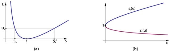  Figure 1. (a) Left picture: in this figure, it is assumed that $s_{*}<1$ (and then $s_{*}<1<s_{*}^{-1}$). On the other hand, when $s_{*}>1$, the position of $s_{*}$ and $s_{*}^{-1}$ is interchanged and $s_{*}^{-1}<1<s_{*}$. (b) Right picture: the function $s_{-}\left(u\right)$ is a monotonically decreasing function in $u\in [0,\infty )$, and then, the function $s_{+}\left(u\right)={\left(s_{-}\left(u\right)\right)}^{-1}$ is a monotonically increasing function of u.
  The functions $s_{\pm }\left(u\right)$ are depicted in Figure 1b. Observe that $s_{+}\left(u\right)s_{-}\left(u\right)=1$. The minimum value of $u\left(s\right)$ is attained at $s=1$ and its value is $u=0$.
  This second change of variable determines different integration regions in the new variable u depending on the value of the upper integration limit in (3),

  $$s_{*}:=t\sqrt{\frac{x}{y}}.$$
  When $s_{*}<1$, the integration variable u in (3) runs from $u=\infty$ to $u=u_{*}=u\left(s_{*}\right)$ (with $s\left(u\right)=s_{-}\left(u\right)$, see Figure 1). On the other hand, when $s_{*}>1$, the position of $s_{*}$ and $s_{*}^{-1}$ is interchanged in Figure 1, and then, the integration variable u in (3) runs from $u=\infty$ to $u=0$ (with $s\left(u\right)=s_{-}\left(u\right)$) and also from $u=0$ to $u=u_{*}$ (with $s\left(u\right)=s_{+}\left(u\right)$). Then, when $s_{*}<1$, only $s_{-}\left(u\right)$ is required in the computation. However, when $s_{*}>1$, then both, $s_{+}\left(u\right)$ and $s_{-}\left(u\right)$ are involved. It is clear from Figure 1 that

  $$S_t\left[g\right](x,y)=e^{-2\sqrt{xy}}\left\{\begin{array}{c}{\int }_{u_{*}}^{\infty }{e}^{-2\sqrt{xy}u}g\left(\sqrt{\frac{y}{x}}{s}_{-}\left(u\right)\right)\frac{du}{\sqrt{u(2+u)}},\mathrm{if}t\le \sqrt{\frac{y}{x}},\hfill \\ {\int }_0^{\infty }{e}^{-2\sqrt{xy}u}g\left(\sqrt{\frac{y}{x}}{s}_{-}\left(u\right)\right)\frac{du}{\sqrt{u(2+u)}}\hfill \\ +{\int }_0^{u_{*}}{e}^{-2\sqrt{xy}u}g\left(\sqrt{\frac{y}{x}}{s}_{+}\left(u\right)\right)\frac{du}{\sqrt{u(2+u)}},\mathrm{if}t>\sqrt{\frac{y}{x}},\hfill \end{array}\right.$$

  (4)

  where

  $$u_{*}:=u\left(s_{*}\right)=\frac{1}{2}\left[t\sqrt{\frac{x}{y}}+\frac{1}{t}\sqrt{\frac{y}{x}}\right]-1\ge 0.$$
• Third change of variable. The two integrals in the second and third lines of (4) are suitable for an asymptotic analysis when $xy$ is large by using Watson’s lemma ([14], Chap. 2); a brief and simple version of Watson’s lemma is summarized in Appendix A. This is so because the maximum value of the exponent in the integration interval is attained at $u=0$, which is the left end point of the integration interval, and only the factor $\sqrt{u}$ in the denominator of these integrals vanishes at this point, whereas the other factor $\sqrt{2+u}$ is analytic there. The situation is different for the integral in the first line of (4). Once again, the maximum value of the exponent in the integration interval is attained at $u=u_{*}$, which is the left end point of the integration interval. However, now, although the whole denominator $\sqrt{u(2+u)}$ is analytic there, when the variable t approaches the critical value $\sqrt{y/x}$ ($s_{*}$ approaches the critical value 1), the integration limit $u_{*}$ approaches the value zero, where $\sqrt{u(2+u)}$ vanishes. Therefore, in the two last integrals, an expansion of the integrand at the asymptotically relevant point $u=0$ is possible for any value of t, and Watson’s lemma can be applied uniformly in the time variable t. On the other hand, in the first integral, this expansion is only possible when the time variable t is bounded away from the critical time

  $$t_{*}:=\sqrt{y/x}.$$
  It is assumed in this discussion that as a function of the variable u, the “composite” pumping function

  $$g\left(\sqrt{\frac{y}{x}}{s}_{\pm }\left(u\right)\right)$$

  is analytic at $u=u_{*}$ for any value of $t>0$. This assumption does not mean any restriction from a practical point of view, as any realistic pumping function meets this condition. Nevertheless, the specific requirements for the pumping function will be established below.
  As an asymptotic expansion of the Moench transform uniformly valid in $t\in [0,\infty )$ is sought, the above-mentioned problem needs to be solved. The solution is a third change of variable $u\to s$ with $u=s^2$. In order to simplify the notation, the following functions are defined

  $${\alpha }_{\pm }\left(s\right):=1+s^2\pm s\sqrt{2+s^2},$$

  (5)

  and the parameter

  $$\mathsf{\Lambda }(x,y,t):=\sqrt{\frac{1}{2}\left[t\sqrt{\frac{x}{y}}+\frac{1}{t}\sqrt{\frac{y}{x}}\right]-1}\ge 0.$$

  (6)
  Then, introducing the change of variable $u=s^2$ in (4),

  $$S_t\left[g\right](x,y)=2e^{-2\sqrt{xy}}\left\{\begin{array}{c}{\int }_{\mathsf{\Lambda }}^{\infty }{e}^{-2\sqrt{xy}{s}^2}g\left(\sqrt{\frac{y}{x}}{\alpha }_{-}\left(s\right)\right)\frac{ds}{\sqrt{2+s^2}},\mathrm{if}t\le t_{*},\hfill \\ {\int }_0^{\infty }{e}^{-2\sqrt{xy}{s}^2}g\left(\sqrt{\frac{y}{x}}{\alpha }_{-}\left(s\right)\right)\frac{ds}{\sqrt{2+s^2}}\hfill \\ +{\int }_0^{\mathsf{\Lambda }}{e}^{-2\sqrt{xy}{s}^2}g\left(\sqrt{\frac{y}{x}}{\alpha }_{+}\left(s\right)\right)\frac{ds}{\sqrt{2+s^2}},\mathrm{if}t>t_{*}.\hfill \end{array}\right.$$
  The asymptotic features of the three integrals have not changed, but now, the factor $1/\sqrt{2+s^2}$ (in the three integrals) is analytic at the asymptotic relevant point $s=0$ (in the two last integrals) and $s=\mathsf{\Lambda }$ (in the first one), even when $t\to \sqrt{y/x}$ and $\mathsf{\Lambda }\to 0$. However, before proceeding further and apply Watson’s lemma to these integrals, a more compact form of $S_t\left[g\right](x,y)$ that simplifies computations is considered,

  $$\begin{array}{cc}\hfill S_t\left[g\right](x,y)=2e^{-2\sqrt{xy}}& \left\{{\int }_0^{\infty }{e}^{-2\sqrt{xy}{s}^2}g\left(\sqrt{\frac{y}{x}}{\alpha }_{-}\left(s\right)\right)\frac{ds}{\sqrt{2+s^2}}\right.\hfill \\ \\ & \left.+\chi \left(t\right){\int }_0^{\mathsf{\Lambda }}{e}^{-2\sqrt{xy}{s}^2}g\left(\sqrt{\frac{y}{x}}{\alpha }_{\chi }\left(s\right)\right)\frac{ds}{\sqrt{2+s^2}}\right\},\hfill \end{array}$$

  (7)

  where we have introduced the step function $\chi \left(t\right)$ and the sign function $\chi$:

  $$\chi \left(t\right):=\left\{\begin{array}{cc}\hfill 1& \mathrm{if}t>t_{*},\hfill \\ \\ \hfill -1& \mathrm{if}t<t_{*},\hfill \end{array}\right.\chi :=\mathrm{sign}\left(t-t_{*}\right)=\left\{\begin{array}{cc}\hfill +& \mathrm{if}t>t_{*},\hfill \\ \\ \hfill -& \mathrm{if}t<t_{*}.\hfill \end{array}\right.$$

Either of the two integrals in (7) has the form of a Laplace transform, which is suitable for an asymptotic analysis when $xy$ is large by using Watson’s lemma ([14], Chap. 2) for any value of $t\ge 0$, whenever the asymptotic expansion of $g\left(\sqrt{y/x}{\alpha }_{\pm }\left(s\right)\right)$ at $s=0$ is uniformly valid for large x and bounded values of y. The two integrals in (7) shall be studied separately. However, for the sake of clarity, and because it is more common in practice [9], in the next section, the particular case of a pumping function $g\left(u\right)$ of power type is considered: $g\left(u\right)=u^{\nu }$, and the study of a general pumping function $g\left(u\right)$ is relegated to the Appendix B. As it will be seen below, in the case of a pumping function of power type, the coefficients of the asymptotic expansion of $g\left(\sqrt{y/x}{\alpha }_{\pm }\left(s\right)\right)$ may be computed explicitly and do not depend on the parameters x, y (and then, it is trivially uniform in these variables), whereas in the case of a general pumping function, the asymptotic expansion of $g\left(\sqrt{y/x}{\alpha }_{\pm }\left(s\right)\right)$ must be written in terms of arbitrary coefficients, and their dependence on the parameters x, y must be analyzed.

3. Asymptotic Approximation of (7) for a Pumping Function of Power Type

Setting $g\left(u\right)=u^{\nu }$ in (7), the Moench transform of this pumping function reads

$$S_t\left[u^{\nu }\right](x,y)=2e^{-2\sqrt{xy}}{\left(\frac{y}{x}\right)}^{\frac{\nu }{2}}\left\{{\int }_0^{\infty }{e}^{-2\sqrt{xy}{s}^2}{h}_{-}\left(s\right)ds+\chi \left(t\right){\int }_0^{\mathsf{\Lambda }}{e}^{-2\sqrt{xy}{s}^2}{h}_{\chi }\left(s\right)ds\right\},$$

(8)

where

$$h_{\pm }\left(s\right):=\frac{{\left({\alpha }_{\pm }\left(s\right)\right)}^{\nu }}{\sqrt{2+s^2}},$$

(9)

with ${\alpha }_{\pm }\left(s\right)$ given in (5). From [14], Watson’s lemma can be applied to the two integrals above whenever the two functions $h_{\pm }\left(s\right)$ are infinitely differentiable at $s=0$, and their derivatives are uniformly bounded by a positive constant times an exponential function $e^{b{s}^2}$, with $b<2\sqrt{xy}$. From the definition (5) of the functions ${\alpha }_{\pm }\left(s\right)$, it is clear that both functions $h_{\pm }\left(s\right)$ are infinitely differentiable at $s=0$, and their derivatives are power functions bounded by a positive constant times an exponential $e^{b{s}^2}$ for any $b>0$. In order to apply Watson’s lemma, the asymptotic expansion of $h_{\pm }\left(s\right)$ needs to be considered at $s=0$ ([14], Chap. 2),

$$h_{\pm }\left(s\right)\sim \sum _{k=0}^{\infty }{c}_k^{\pm }{s}^k.$$

(10)

The coefficients $c_k^{\pm }$ may be computed by using a symbolic manipulator. They may also be computed by means of a recurrence relation. In order to derive this recurrence, the above expansion must be introduced into the following differential equation satisfied by $h_{\pm }\left(s\right)$,

$$(2+s^2)h_{\pm }^{\prime }+(s\mp 2\nu \sqrt{2+s^2})h_{\pm }=0.$$

After some simplifications, and equating the coefficients of equal powers of s, it can be checked that the coefficients $c_n$ satisfy the recurrence relation

$$c_{n+1}^{\pm }=\frac{1}{2(n+1)}\left[-n{c}_{n-1}^{\pm }\pm 2\sqrt{2}\nu \sum _{k=0}^{\lfloor n/2\rfloor }\left(\genfrac{}{}{0pt}{}{1/2}{k}\right)\frac{1}{2^k}{c}_{n-2k}^{\pm }\right],$$

$n=1,2,3,\dots$, with

$$c_0^{\pm }=\frac{1}{\sqrt{2}},c_1^{\pm }=\pm \nu .$$

The first few coefficients of the expansion are

$$h_{\pm }\left(s\right)\sim \frac{1}{\sqrt{2}}\pm \nu s+\frac{4{\nu }^2-1}{4\sqrt{2}}{s}^2\pm \frac{\nu ({\nu }^2-1)}{3}{s}^3+\frac{\sqrt{2}(16{\nu }^4-40{\nu }^2+9)}{192}{s}^4+\cdots$$

From Watson’s lemma ([14], Chap. 2), an asymptotic expansion of (8) for large $xy$ follows by introducing the expansion (10) into the two integrals on the right-hand side of (8) and interchanging the sum and integral. For the first integral, the asymptotic expansion is given by

$${\int }_0^{\infty }{e}^{-2\sqrt{xy}{s}^2}{h}_{-}\left(s\right)ds\sim \sum _{k=0}^{\infty }{c}_k^{-}{\int }_0^{\infty }{e}^{-2\sqrt{xy}{s}^2}{s}^{k}ds,$$

(11)

and for the second one,

$${\int }_0^{\mathsf{\Lambda }}{e}^{-2\sqrt{xy}{s}^2}{h}_{\pm }\left(s\right)ds\sim \sum _{k=0}^{\infty }{c}_k^{\pm }{\mathsf{\Phi }}_k(x,y,t),$$

(12)

with

$${\mathsf{\Phi }}_k(x,y,t):={\int }_0^{\mathsf{\Lambda }}{e}^{-2\sqrt{xy}{s}^2}{s}^{k}ds.$$

(13)

The integrals in the asymptotic expansion (11) may be computed exactly in terms of elementary functions,

$${\int }_0^{\infty }{e}^{-2\sqrt{xy}{s}^2}{s}^{k}ds=\frac{1}{2}\frac{\mathsf{\Gamma }\left(\frac{k+1}{2}\right)}{\sqrt{{\left(2\sqrt{xy}\right)}^{k+1}}}.$$

(14)

For the values of z required in the above formula, we have that

$$\mathsf{\Gamma }\left(\frac{2k+1}{2}\right)=\frac{(2k-1)!!}{2^k}\sqrt{\pi },\mathsf{\Gamma }(k+1)=k!,k=0,1,2,\dots ,$$

where $\left(n\right)!!$ denotes the double factorial of the integer number $n=-1,0,1,2,\dots$ ([22], Equation 5.4.2) with $(-1)!!=\left(0\right)!!=1$.

On the other hand, the computation of the integrals (13) in the asymptotic expansion (12) is more elaborated. Integrating by parts in the integral (13), it is straightforward to obtain the recurrence relation

$${\mathsf{\Phi }}_{k+1}(x,y,t)=\frac{k}{4\sqrt{xy}}{\mathsf{\Phi }}_{k-1}(x,y,t)-\frac{{\mathsf{\Lambda }}^k}{4\sqrt{xy}}{e}^{-2\sqrt{xy}{\mathsf{\Lambda }}^2},k=1,2,3,\dots$$

(15)

with

$${\mathsf{\Phi }}_0(x,y,t)=\frac{\sqrt{\pi }}{2\sqrt{2\sqrt{xy}}}\mathrm{erf}\left(\mathsf{\Lambda }\sqrt{2\sqrt{xy}}\right),{\mathsf{\Phi }}_1(x,y,t)=\frac{1-e^{-2\sqrt{xy}{\mathsf{\Lambda }}^2}}{4\sqrt{xy}},$$

where $\mathrm{erf}\left(z\right)$ is the well-known error function [23] that models fast but continuous transitions between two constant values. The solution to the recurrence relation (15) is, for $n=0,1,2,3,\dots$,

$$\begin{array}{cc}\hfill {\mathsf{\Phi }}_n(x,y,t)=& \frac{(n-1)!!}{{\left(4\sqrt{xy}\right)}^{(n+1)/2}}\left[\frac{1-{(-1)}^n}{2}+\frac{(1+{(-1)}^n)}{2}\sqrt{\frac{\pi }{2}}\mathrm{erf}\left(\mathsf{\Lambda }\sqrt{2\sqrt{xy}}\right)\right.\hfill \\ \\ \hfill & \left.-e^{-2{\mathsf{\Lambda }}^2\sqrt{xy}}\sum _{k=0}^{\lfloor (n-1)/2\rfloor }\frac{{\left(4{\mathsf{\Lambda }}^2\sqrt{xy}\right)}^{(n-1)/2-k}}{(n-1-2k)!!}\right],\hfill \end{array}$$

(16)

where empty sums must be understood as zero.

Therefore, from (8), (11), (12), (14) and (16), the following asymptotic expansion of the Moench transform for pumping functions of power type is finally derived,

$$S_t\left[u^{\nu }\right](x,y)\sim e^{-2\sqrt{xy}}{\left(\frac{y}{x}\right)}^{\frac{\nu }{2}}\sum _{n=0}^{\infty }\frac{{\mathsf{\Psi }}_n(x,y,t)}{{\left(2\sqrt{xy}\right)}^{(n+1)/2}},$$

(17)

where for $n=0,1,2,\dots$, the sequence of functions ${\mathsf{\Psi }}_n(x,y,t)$ is defined in the form

$$\begin{array}{cc}\hfill & {\mathsf{\Psi }}_n(x,y,t)=c_n^{-}\mathsf{\Gamma }\left(\frac{n+1}{2}\right)+\chi \left(t\right)c_n^{\chi }\frac{(n-1)!!}{{\left(\sqrt{2}\right)}^{n+1}}[1-{(-1)}^n\hfill \\ \\ \hfill & \left.+(1+{(-1)}^n)\sqrt{\frac{\pi }{2}}\mathrm{erf}\left(\mathsf{\Lambda }\sqrt{2\sqrt{xy}}\right)-2e^{-2{\mathsf{\Lambda }}^2\sqrt{xy}}\sum _{k=0}^{\lfloor (n-1)/2\rfloor }\frac{{\left(4{\mathsf{\Lambda }}^2\sqrt{xy}\right)}^{(n-1)/2-k}}{(n-1-2k)!!}\right],\hfill \end{array}$$

(18)

where empty sums (for $n=0$) must be understood as zero.

Observe from (18) that the functions ${\mathsf{\Psi }}_n(x,y,t)$ depend on the variables $x,y,t$ through the combination ${\mathsf{\Lambda }}^2\sqrt{xy}$. Moreover, the right-hand side of (18) is a sum of constants, an error function (whose absolute value is bounded by 1) and terms of the form ${\left({\mathsf{\Lambda }}^2\sqrt{xy}\right)}^k{e}^{-2{\mathsf{\Lambda }}^2\sqrt{xy}}$, all of them bounded for any value of ${\mathsf{\Lambda }}^2\sqrt{xy}\in [0,\infty )$. Therefore, the numerators ${\mathsf{\Psi }}_n(x,y,t)$ in terms of the expansion (17) are bounded functions of ${\mathsf{\Lambda }}^2\sqrt{xy}$, which means that the terms of the expansion (17) are of the order $\mathcal{O}\left({\left(\sqrt{xy}\right)}^{-(n+1)/2}\right)$ when $\sqrt{xy}\to \infty$ uniformly in the time variable $t\in [0,\infty )$.

In particular, the first-order approximation (obtained by considering only the first term $n=0$ of the sum (17)) is given by the following formula:

$$S_t\left[u^{\nu }\right](x,y)\sim \frac{\sqrt{\pi }{e}^{-2\sqrt{xy}}}{2{\left(xy\right)}^{1/4}}{\left(\frac{y}{x}\right)}^{\frac{\nu }{2}}\left[1+\mathrm{sign}\left(t-\sqrt{\frac{y}{x}}\right)\mathrm{erf}\left(\sqrt{tx+\frac{y}{t}-2\sqrt{xy}}\right)\right].$$

(19)

The accuracy of Formula (19) is illustrated in Figure 2.

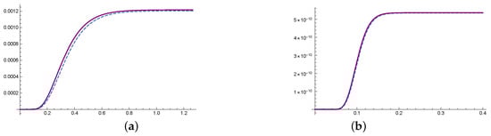
Figure 2. The dashed line represents the integral $S_t\left[u^{1/3}\right](x,1)$ as a function of t. The purple line corresponds to the approximation for $n=0$ (19) with $x=10$ (a) and $x=100$ (b).

The argument of the error function on the right-hand side of (19) (and also in all the error functions in the successive terms of the expansion (17)) is $2\mathsf{\Lambda }\sqrt{xy}$, where $\mathsf{\Lambda }$ is defined in (6). At the critical value $t=t_{*}=\sqrt{y/x}$, we have that $\mathsf{\Lambda }=0$, and then this error function, multiplied by the sign function, presents a fast transition from the value $-1$ to the value 1 as t crosses this critical value $t_{*}$. Then, this function encodes the fast (but smooth) transition that Moench’s transform experiments at the critical time $t=t_{*}$, from a value close to the zero value (as $S_0\left[u^{\nu }\right](x,y)=0$) to a value close to

$$S_{\infty }\left[u^{\nu }\right](x,y)=\frac{\sqrt{\pi }{e}^{-2\sqrt{xy}}}{{\left(xy\right)}^{1/4}}{\left(\frac{y}{x}\right)}^{\frac{\nu }{2}}.$$

It is shown in Figure 2.

4. Numerical Experiments

In Figure 2, the accuracy of Formula (19) (particular case of Formula (17)) for certain selected values of the parameters x, y, $\nu$ is shown. In this section, one step forward is given, and the accuracy of the approximation (17) in a more realistic situation is shown. Consider the experimental data obtained from the experiment described in Part 3 of [9] that was conducted by Layne-Western Company on 2 July 1953 on a village well at Gridley, McLean County, Illinois (for more details, see Part 3 in [9]). For this experiment, the parameter values are $T=$ 10,100 gpd/ft $=0.9378$ feet${}^2/$min, $S=0.00002$, $r=824$ feet, $P/m=560/18$ gpd/feet${}^3=2.8886\times {10}^{-3}$ min${}^{-1}$, and a pumping function $g\left(u\right)=220$ gpm $=29.414$ feet${}^3/$min. These parameter values translate into the values $(x,y)=(P/\left(2m\right),S{r}^2/\left(4T\right))=(144.429,3.6202)$ used in Moench’s transform $S_t\left[g\right](x,y)$.

In Table 1, Table 2, Table 3 and Table 4, the absolute value of the relative error obtained by using the approximation given by (17) is computed when $t\ge \sqrt{y/x}=0.1583$ (to the right of the critical time), when $t<\sqrt{y/x}=0.1583$ (to the left of the critical time) and when $t\simeq \sqrt{y/x}=0.1583$ (near the critical time), for several values of the degree n of the approximation and the above values of x and y. In every table, four different values of the time t and a pumping function of the form $g\left(t\right)=220t^{\nu }$ are considered with a different value of $\nu$ in every table. Four different values for $\nu$ are considered: $\nu =0$ to exactly reproduce Moench’s theory, and three other values that represent certain Vanderberg-type modifications, with $\nu =-1/2,1/2$ and $1/8$. All the computations in the tables and figures have been carried out by using the symbolic manipulation software Wolfram Mathematica 12.2. In particular, the “exact” value of the integral $S_t\left[g\right](x,y)$ defined in (2) was computed by means of numerical integration with the command NIntegrate.

Table 1. Pumping function $g\left(t\right)=220$ and $t_{*}=0.1583$.

n	$\mathit{t}=0.08$	$\mathit{t}={\mathit{t}}_{*}$	$\mathit{t}=5.0$	$\mathit{t}=50.0$
0	6.37 × 10${}^{-2}$	2.75 × 10${}^{-2}$	2.70 × 10${}^{-3}$	2.70 × 10${}^{-3}$
2	6.26 × 10${}^{-3}$	3.34 × 10${}^{-5}$	3.30 × 10${}^{-5}$	3.30 × 10${}^{-5}$
4	6.92 × 10${}^{-4}$	7.54 × 10${}^{-7}$	7.43 × 10${}^{-7}$	7.43 × 10${}^{-7}$
6	8.11 × 10${}^{-5}$	2.50 × 10${}^{-8}$	2.47 × 10${}^{-8}$	2.46 × 10${}^{-8}$

Table 2. Pumping function $g\left(t\right)=220t^{-1/2}$ and $t_{*}=0.1583$.

n	$\mathit{t}=0.08$	$\mathit{t}={\mathit{t}}_{*}$	$\mathit{t}=5.0$	$\mathit{t}=50.0$
0	0.25	5.62 × 10${}^{-2}$	4.59 × 10${}^{-11}$	5.93 × 10${}^{-13}$
2	1.62 × 10${}^{-2}$	3.04 × 10${}^{-4}$	4.59 × 10${}^{-11}$	5.93 × 10${}^{-13}$
4	1.60 × 10${}^{-3}$	4.93 × 10${}^{-6}$	4.59 × 10${}^{-11}$	5.93 × 10${}^{-13}$
6	1.78 × 10${}^{-4}$	1.33 × 10${}^{-8}$	4.59 × 10${}^{-11}$	5.93 × 10${}^{-13}$

Table 3. Pumping function $g\left(t\right)=220t^{1/2}$ and $t_{*}=0.1583$.

n	$\mathit{t}=0.08$	$\mathit{t}={\mathit{t}}_{*}$	$\mathit{t}=5.0$	$\mathit{t}=50.0$
0	0.52	6.33 × 10${}^{-2}$	6.30 × 10${}^{-11}$	5.87 × 10${}^{-13}$
2	3.30 × 10${}^{-2}$	3.42 × 10${}^{-4}$	6.30 × 10${}^{-11}$	5.87 × 10${}^{-13}$
4	3.26 × 10${}^{-3}$	5.56 × 10${}^{-6}$	6.30 × 10${}^{-11}$	5.87 × 10${}^{-13}$
6	3.61 × 10${}^{-4}$	1.50 × 10${}^{-7}$	6.30 × 10${}^{-11}$	5.87 × 10${}^{-13}$

Table 4. Pumping function $g\left(t\right)=220t^{1/8}$ and $t_{*}=0.1583$.

n	$\mathit{t}=0.08$	$\mathit{t}={\mathit{t}}_{*}$	$\mathit{t}=5.0$	$\mathit{t}=50.0$
0	0.16	1.77 × 10${}^{-2}$	2.54 × 10${}^{-3}$	2.54 × 10${}^{-3}$
2	1.46 × 10${}^{-2}$	1.39 × 10${}^{-4}$	3.07 × 10${}^{-5}$	3.07 × 10${}^{-5}$
4	1.57 × 10${}^{-3}$	2.56 × 10${}^{-6}$	6.90 × 10${}^{-7}$	6.90 × 10${}^{-7}$
6	1.81 × 10${}^{-4}$	7.50 × 10${}^{-8}$	2.28 × 10${}^{-8}$	2.28 × 10${}^{-8}$

5. Conclusions

A complete asymptotic expansion of Moench’s transform (2) for large values of the parameter x with y bounded from below (or large values of $xy$) that is uniformly valid in the time variable $t\in [0,\infty )$ is derived. It is given in (17) for the particular case (and more interesting in practice) of a power-type pumping function. For a more general pumping function, a complete asymptotic expansion of the Moench transform is given in Appendix B in Formula (A6). In any case, the expansion is given in terms of elementary functions and an error function with fixed argument $2\mathsf{\Lambda }\sqrt{xy}$. For a power-type pumping function, Moench’s transform, which measures the water level in the aquifer, experiences a fast (but continuous) transition between a low level and a top limit level: more precisely, from the zero value attained at $t=0$ ($S_0\left[u^{\nu }\right](x,y)=0$) to the limit value attained at $t=\infty$,

$$S_{\infty }\left[u^{\nu }\right](x,y)=\frac{\sqrt{\pi }{e}^{-2\sqrt{xy}}}{{\left(xy\right)}^{1/4}}{\left(\frac{y}{x}\right)}^{\frac{\nu }{2}}.$$

In the case of a more general pumping function $g\left(u\right)$, the transition is similar but with the factor ${\left(\frac{y}{x}\right)}^{\frac{\nu }{2}}$ replaced by $\frac{1}{2}g\left(\sqrt{\frac{y}{x}}\right)$. This transition occurs around the critical time $t_{*}=\sqrt{y/x}$, where the Moench transform takes half of its maximum value, $S_{t_{*}}\left[g\right](x,y)=\frac{1}{2}{S}_{\infty }\left[g\right](x,y)$. This fast but smooth transition is encoded in the error function that appears in the expansions (17) or (A6) at any order n of the approximation, as all the terms ${\mathsf{\Psi }}_n(x,y,z)$ on the right-hand side of (17) or (A6) contain the error function. The argument of this error function is (see (18) and (6))

$$\mathsf{\Lambda }\sqrt{2\sqrt{xy}}=\sqrt{tx+\frac{y}{t}-2\sqrt{xy}},$$

that vanishes at $t=t_{*}=\sqrt{y/x}$, and precisely the error function experiences the above-mentioned transition when its argument vanishes. Moreover, the larger x is, the faster the transition is, as small variations of the time t around the critical value $t_{*}$ are amplified by the factor x.

The approximations (17) or (A6) have been tested by means of numerical examples that consider realistic parameter values, corresponding to actual physical experiments (see Section 4). As it can be observed in Figure 2 and Figure A1 and Table 1, Table 2, Table 3 and Table 4, the accuracy of the approximations is remarkable.

We have analyzed Moench’s transform for large values of the parameter x with y bounded from below and $t\in [0,\infty )$. It would be interesting to find other approximations of Moench’s transform valid in new regions of the parameters, such as small values of x and/or y. Moreover, it would be interesting to find approximations uniformly valid for x and/or y in $[0,\infty )$. This is the subject of future research.

References

- Hantush, M.S. Analysis of data from pumping tests in leaky aquifers. Trans. Am. Geophys. Union 1956, 37, 702–714. [Google Scholar] [CrossRef]
- Hantush, M.S. Nonsteady flow to flowing wells in leaky aquifers. J. Geophys. Res. 1959, 64, 1043–1052. [Google Scholar] [CrossRef]
- Hantush, M.S. Modification of the theory of leaky aquifers. J. Geophys. Res. 1960, 65, 3713–3725. [Google Scholar] [CrossRef]
- Hantush, M.S.; Jacob, C.E. Non-steady radial flow in an infinit leaky aquifer. Trans. Am. Geophys. Union 1955, 36, 95–100. [Google Scholar] [CrossRef]
- Lohman, S.W. Ground-Water Hidraulics; U.S. Department of the Interior: Washington, DC, USA, 1972.
- Moench, A. Ground-water fluctuations in response to arbitrary pumping. Groundwater 1971, 9, 4–8. [Google Scholar] [CrossRef]
- Stallman, R.W. Variable discharge without vertical leakage. In Theory of Aquifer Tests; Ferris, J.G., Ed.; U. S. Geological Survey Water-Supply Paper 1536-E; US Government Printing Office: Washington, DC, USA, 1962; pp. 118–122. [Google Scholar]
- Theis, C.V. The relation between lowering of the piezometric surface and the rate and duration of discharge of a well using ground-water storage. Trans. Am. Geophys. Union 1935, 2, 519–524. [Google Scholar] [CrossRef]
- Walton, W.C. Selected Analytical Methods for Well and Aquifer Evaluation; Bulletin (Illinois State Water Survey) No. 49; Department of Registration and Education, State Water Survey Division, State of Illinois: Springfield, IL, USA, 1962.
- Hantush, M.S. Drawdown around a partially penetrating well. J. Hyd. Div. Proc. Am. Soc. Civil Eng. 1961, 87, 83–98. [Google Scholar] [CrossRef]
- Hantush, M.S. Aquifer tests on partially penetrating wels. J. Hyd. Div. Proc. Am. Soc. Civil Eng. 1961, 87, 171–194. [Google Scholar]
- Vandenberg, A. Tables and Type Curves for Analysis of Pump Tests in Leaky Parallel-Channel Aquifers; Technical Bulletin No. 96; Inland Waters Directorate, Water Resources Brach: Ottawa, ON, USA, 1976; 28p.
- Vandenberg, A. Type curves for analysis of pump tests in leaky strip aquifers. J. Hydrol. 1977, 33, 15–26. [Google Scholar] [CrossRef]
- Temme, N.M. Asymptotic Methods for Integrals; World Scientific: Singapore, 2015. [Google Scholar]
- Krätzel, E. Integral transformations of Bessel type. In Generalized Functions and Operational Calculus (Proc. Conf., Varna, 1975); Bulgar. Acad. Sci.: Sofia, Bulgaria, 1979. [Google Scholar]
- Harris, F.E. On Kryachko’s formula for the leaky aquifer function. Int. J. Quantum Chem. 2001, 81, 332–334. [Google Scholar] [CrossRef]
- Kryachko, E.S. Explicit expression for the leaky aquifer function. Int. J. Quantum Chem. 2000, 78, 303–305. [Google Scholar] [CrossRef]
- Harris, F.E. New approach to calculation of the leaky aquifer function. Int. J. Quantum Chem. 1997, 63, 913–916. [Google Scholar] [CrossRef]
- Harris, F.E. More about the leaky aquifer function. Int. J. Quantum Chem. 1998, 70, 623–626. [Google Scholar] [CrossRef]
- Chaudhry, M.A.; Temme, N.M.; Veling, E.J.M. Asymptotics and closed form of a generalized incomplete gamma function. J. Comput. Appl. Math. 1996, 67, 371–379. [Google Scholar]
- Harris, F.E. Incomplete Bessel, generalized incomplete gamma, or leaky aquifer function. J. Comput. Appl. Math. 2008, 215, 260–269. [Google Scholar] [CrossRef]
- Askey, R.A.; Roy, R. Gamma Function. In NIST Handbook of Mathematical Functions; Cambridge University Press: Cambridge, UK, 2010; Chapter 5; pp. 135–147. [Google Scholar]
- Temme, N.M. Error Functions, Dawson’s and Fresnel Integrals. In NIST Handbook of Mathematical Functions; Cambridge University Press: Cambridge, UK, 2010; Chapter 7; pp. 160–170. [Google Scholar]
- Di Bruno, F.F. Theorie des Formes Binaires; Librarie Brero: Torino, Italy, 1876. [Google Scholar]
Disclaimer/Publisher’s Note: The statements, opinions and data contained in all publications are solely those of the individual author(s) and contributor(s) and not of MDPI and/or the editor(s). MDPI and/or the editor(s) disclaim responsibility for any injury to people or property resulting from any ideas, methods, instructions or products referred to in the content. |
© 2023 by the authors. Licensee MDPI, Basel, Switzerland. This article is an open access article distributed under the terms and conditions of the Creative Commons Attribution (CC BY) license (https://creativecommons.org/licenses/by/4.0/).