Analysis of an Integrated Pest Management Model with Impulsive Diffusion between Two Regions

Abstract

This paper investigates an integrated pest management model with pulsed diffusion. As we all know, humans have been fighting against pests since they entered the age of farming. When pests are controlled, humans can achieve better harvests. We use the stroboscopic mapping of discrete dynamic system to obtain some important lemmas. Based on the lemmas, firstly, we give the conditions for the global asymptotic stability of the periodic solution of the pest eradication boundary; secondly, the conditions for the permanence of the investigated system are derived; thirdly, numerical simulations are used to verify our obtained theoretical results; finally, increased dispersal was found to have the opposite effect on integrated pest management. We conclude that a combination of impulsive diffusion, spraying pesticides, and releasing natural enemies can play a crucial role in integrated pest management.

1. Introduction

Integrated pest management (IPM) is a management system for pests which uses appropriate techniques and methods as cooperatively as possible in the light of the population dynamics of pests and their related environmental relationships, so that pest populations can be kept below the level of economic harm. By using an integrated pest management approach, we can effectively manage pests while minimizing the negative impact on the environment. The measures taken by integrated pest management mainly include tools of chemical control, biological control, cultural control, mechanical or physical control, genetic control, etc. In recent years, the models of integrated pest management have been extensively and deeply studied by many scholars [1,2,3,4,5,6,7,8,9,10,11,12,13,14,15,16,17,18].

In 1972, the United States Council on Environmental Quality proposed the concept of “integrated pest management” (IPM). In terms of the definition of the Food and Agriculture Organization of the United Nations: Integrated management is a pest management system that keeps pest populations below economic hazard levels in accordance with the population dynamics of pests and the environmental relationships associated with them, using appropriate techniques and control methods in as coordinated a manner as possible [19].

According to the definition of IPM, the aim of integrated control is to control pest populations within a certain number, so that the damage caused by pests is below the economically permissible level, rather than to eliminate pests completely. This means that measures to control the growth of pests are implemented only when pest populations reach a certain level (i.e., a critical level) and cause damage to crops that humans cannot tolerate. This so-called critical level is the “economic threshold” (ET) in pest management [20]. Biological control serves as an ecological management strategy aimed at regulating the population of host pests, rather than eradicating them entirely. The objective is to maintain the number of host pests below the economically significant threshold, which ensures the survival of natural enemies and restores a favorable ecological balance in farmland. Ultimately, this approach maximizes benefits and promotes a harmonious agricultural ecosystem [20]. In crops, the presence of a small number of pests can provide food and intermediate hosts for natural enemies, thereby increasing the natural control ability of natural enemies. For example, if the number of leaf-eating pests in rice fields is controlled (less than ET), it is the intermediate host of the parasitic bee of rice bracts, red-eyed bees, and their presence can maintain the number of red-eyed bees. If they all are killed, rice bracts will be flooded in the later stages of the rice field [20].

In this paper, we investigate a pest management model with impulsive diffusion, spraying pesticides, and releasing natural enemies. We aim to uncover the dynamical properties of the system under investigation. Additionally, we anticipate that employing impulsive diffusion, spraying pesticides, and releasing natural enemies will establish a solid foundation for effective pest management.

The structure of this paper is outlined as follows. In Section 2, we introduce the model and provide some background concepts. Section 3 presents several important lemmas. In Section 4, we examine the globally asymptotically stable conditions for the periodic solution of system (1) at the pest eradication boundary, along with the permanent conditions of system (1). In Section 5, we present simulation analyses and offer a brief discussion. Finally, we obtain a concluding statement regarding integrated pest management to summarize our findings.

2. The Model

Based on the basic principles of pest control [1,7,11], in this paper, we hypothesize that the system consists of two patches connected by diffusion, which are divided by rivers, highways, or railways. Predator populations can transcend rivers, highways, or railways, while pest populations cannot. we build a class of pest management model with pesticide spraying, natural enemies release, and dispersal at different pulse moments as follows:

$$\left\{\begin{array}{c}\left.\begin{array}{c}{\displaystyle \frac{d{x}_1\left(t\right)}{dt}=x_1\left(t\right)(a_1-b_1{x}_1\left(t\right))-{\beta }_1{x}_1\left(t\right)y_1\left(t\right),}\hfill \\ {\displaystyle \frac{d{y}_1\left(t\right)}{dt}=k_1{\beta }_1{x}_1\left(t\right)y_1\left(t\right)-d_1{y}_1\left(t\right),}\hfill \\ {\displaystyle \frac{d{x}_2\left(t\right)}{dt}=x_2\left(t\right)(a_2-b_2{x}_2\left(t\right))-{\beta }_2{x}_2\left(t\right)y_2\left(t\right),}\hfill \\ {\displaystyle \frac{d{y}_2\left(t\right)}{dt}=k_2{\beta }_2{x}_2\left(t\right)y_2\left(t\right)-d_2{y}_2\left(t\right),}\hfill \end{array}\right\}t\ne (n+p)u,t\ne (n+p+q)u,t\ne (n+1)u,\hfill \\ \left.\begin{array}{c}{\displaystyle \Delta x_1\left(t\right)=0,}\hfill \\ {\displaystyle \Delta y_1\left(t\right)=D(y_2\left(t\right)-y_1\left(t\right)),}\hfill \\ {\displaystyle \Delta x_2\left(t\right)=0,}\hfill \\ {\displaystyle \Delta y_2\left(t\right)=D(y_1\left(t\right)-y_2\left(t\right)),}\hfill \end{array}\right\}t=(n+p)u,n\in Z^{+},\hfill \\ \left.\begin{array}{c}{\displaystyle \Delta x_1\left(t\right)=-{\mu }_{11}{x}_1\left(t\right),}\hfill \\ {\displaystyle \Delta y_1\left(t\right)=-{\mu }_{12}{y}_1\left(t\right),}\hfill \\ {\displaystyle \Delta x_2\left(t\right)=-{\mu }_{21}{x}_2\left(t\right),}\hfill \\ {\displaystyle \Delta y_2\left(t\right)=-{\mu }_{22}{y}_2\left(t\right),}\hfill \end{array}\right\}t=(n+p+q)u,n\in Z^{+},\hfill \\ \left.\begin{array}{c}{\displaystyle \Delta x_1\left(t\right)=0,}\hfill \\ {\displaystyle \Delta y_1\left(t\right)={\mu }_1,}\hfill \\ {\displaystyle \Delta x_2\left(t\right)=0,}\hfill \\ {\displaystyle \Delta y_2\left(t\right)={\mu }_2,}\hfill \end{array}\right\}t=(n+1)u,n\in Z^{+},\hfill \end{array}\right.$$

(1)

where $x_i\left(t\right)$ and $y_i\left(t\right)$ denote the densities of the pest and predator populations in patch $i(i=1,2)$ at time t, D represents the dispersal rate of the predator between two patches; it is assumed that the net exchange of the predator from the jth patch to the ith patch is proportional to the difference of $y_j,y_i$ of the predator densities at time $t=(n+p)u$, $0<p<1$, $n\in Z^{+}$. ${\mu }_{11},{\mu }_{12},{\mu }_{21},{\mu }_{22}$ are, respectively, the killing rates of $x_i\left(t\right),y_i\left(t\right),i=1,2$ due to pesticide spraying at time $t=(n+p+q)u$, $0<p+q<1,n\in Z^{+}$. ${\mu }_i(i=1,2)$ is the amount of natural enemies released $y_i(i=1,2)$ at time $t=(n+1)u$. $a_i>0$ represents the intrinsic growth rate of the prey population in patch $i(i=1,2)$, and $b_i>0$ represents the coefficient of the intraspecific competition of the prey population in patch $i(i=1,2)$. $d_i>0$ stands for the natural death rate $i(i=1,2)$, ${\beta }_i(i=1,2)$ is the capture rate of predators in the ith patch, and $k_i(i=1,2)$ is the rate of conversion of nutrients into the reproduction rate of predators in the ith patch [18].

3. The Lemmas

Firstly, similar to the literature [18], we can demonstrate that all solutions of (1) are uniformly ultimately bounded.

Lemma 1. 

For every solution $(x_1\left(t\right),y_1\left(t\right),x_2\left(t\right),y_2\left(t\right))$ of (1), there exists a positive constant M such that $M\ge x_i\left(t\right)$ and $M\ge y_i\left(t\right)$ (where $i=1,2$) for sufficiently large t.

If $x_i\left(t\right)=0$ for $i=1,2$, we have a subsystem of Equation (1).

$$\left\{\begin{array}{c}\left.\begin{array}{c}{\displaystyle \frac{d{y}_1\left(t\right)}{dt}=-d_1{y}_1\left(t\right),}\hfill \\ {\displaystyle \frac{d{y}_2\left(t\right)}{dt}=-d_2{y}_2\left(t\right),}\hfill \end{array}\right\}t\ne (n+p)u,t\ne (n+p+q)u,t\ne (n+1)u,\hfill \\ \left.\begin{array}{c}{\displaystyle \Delta y_1\left(t\right)=D(y_2\left(t\right)-y_1\left(t\right)),}\hfill \\ {\displaystyle \Delta y_2\left(t\right)=D(y_1\left(t\right)-y_2\left(t\right)),}\hfill \end{array}\right\}t=(n+p)u,\hfill \\ \left.\begin{array}{c}{\displaystyle \Delta y_1\left(t\right)=-{\mu }_{12}{y}_1\left(t\right),}\hfill \\ {\displaystyle \Delta y_2\left(t\right)=-{\mu }_{22}{y}_2\left(t\right),}\hfill \end{array}\right\}t=(n+p+q)u,\hfill \\ \left.\begin{array}{c}{\displaystyle \Delta y_1\left(t\right)={\mu }_1,}\hfill \\ {\displaystyle \Delta y_2\left(t\right)={\mu }_2,}\hfill \end{array}\right\}t=(n+1)u,n=1,2,\dots .\hfill \end{array}\right.$$

(2)

The analytic solution of Equation (2) among pulses can be obtained easily as follows.

$$\left\{\begin{array}{c}\begin{array}{c}{\displaystyle y_1\left(t\right)=}\hfill \end{array}\left\{\begin{array}{c}{\displaystyle y_1\left(n{u}^{+}\right)e^{-d_1(t-nu)},t\in (nu,(n+p)u],}\hfill \\ {\displaystyle y_1\left((n+p)u^{+}\right)e^{-d_1(t-(n+p)u)},t\in ((n+p)u,(n+p+q)u],}\hfill \\ y_1\left((n+p+q)u^{+}\right)e^{-d_1(t-(n+p+q)u)},t\in ((n+p+q)u,(n+1)u],\hfill \end{array}\right.\hfill \\ \begin{array}{c}{\displaystyle y_2\left(t\right)=}\hfill \end{array}\left\{\begin{array}{c}{\displaystyle y_2\left(n{u}^{+}\right)e^{-d_2(t-nu)},t\in (nu,(n+p)u],}\hfill \\ {\displaystyle y_2\left((n+p)u^{+}\right)e^{-d_2(t-(n+p)u)},t\in ((n+p)u,(n+p+q)u],}\hfill \\ y_2\left((n+p+q)u^{+}\right)e^{-d_2(t-(n+p+q)u)},t\in ((n+p+q)u,(n+1)u].\hfill \end{array}\right.\hfill \end{array}\right.$$

(3)

Contemplating the third and fourth equations of (2), we have

$$\left\{\begin{array}{c}{\displaystyle y_1\left((n+p)u^{+}\right)=(1-D)e^{-d_{1}pu}{y}_1\left(n{u}^{+}\right)+D{e}^{-d_{2}pu}{y}_2\left(n{u}^{+}\right),}\hfill \\ {\displaystyle y_2\left((n+p)u^{+}\right)=D{e}^{-d_{1}lu}{y}_1\left(n{u}^{+}\right)+(1-D)e^{-d_{2}lu}{y}_2\left(n{u}^{+}\right).}\hfill \end{array}\right.$$

(4)

Contemplating the fifth and sixth equations of (2), we also have

$$\left\{\begin{array}{c}{\displaystyle y_1\left((n+p+q)u^{+}\right)=(1-{\mu }_{12})e^{-d_{1}qu}{y}_1\left((n+p)u^{+}\right),}\hfill \\ {\displaystyle y_2\left((n+p+q)u^{+}\right)=(1-{\mu }_{22})e^{-d_{2}qu}{y}_2\left((n+p)u^{+}\right).}\hfill \end{array}\right.$$

(5)

Contemplating the seventh and eighth equations of (2), we also have

$$\left\{\begin{array}{c}{\displaystyle y_1\left((n+1)u^{+}\right)=y_1\left((n+p+q)u^{+}\right)e^{-d_1(1-p-q)u}+{\mu }_1,}\hfill \\ {\displaystyle y_2\left((n+1)u^{+}\right)=y_2\left((n+p+q)u^{+}\right)e^{-d_2(1-p-q)u}+{\mu }_2.}\hfill \end{array}\right.$$

(6)

By substituting (4) and (5) into (6), we have the stroboscopic map of (2)

$$\left\{\begin{array}{c}{\displaystyle y_1\left((n+1)u^{+}\right)=(1-{\mu }_{12})(1-D)e^{-d_{1}u}{y}_1\left(n{u}^{+}\right)}\hfill \\ +(1-{\mu }_{12})D{e}^{-[d_1(1-p)+d_{2}p]u}{y}_2\left(n{u}^{+}\right)+{\mu }_1,\hfill \\ \\ {\displaystyle y_2\left((n+1)u^{+}\right)=(1-{\mu }_{22})D{e}^{-[d_{1}p+d_2(1-p)]u}{y}_1\left(n{u}^{+}\right)}\hfill \\ +(1-{\mu }_{22})(1-D)e^{-d_{2}u}{y}_2\left(n{u}^{+}\right)+{\mu }_2.\hfill \end{array}\right.$$

(7)

System (7) has one fixed point

$$\left\{\begin{array}{c}{\displaystyle y_1^{*}=\frac{{\mu }_2{F}_1+{\mu }_1(1-F_2)}{(1-E_1)(1-F_2)-E_2{F}_1}>0,}\hfill \\ {\displaystyle y_2^{*}=\frac{{\mu }_1{E}_2+{\mu }_2(1-E_1)}{(1-E_1)(1-F_2)-E_2{F}_1}>0,}\hfill \end{array}\right.$$

(8)

where

$$E_1=(1-{\mu }_{12})(1-D)e^{-d_{1}u}<1,$$

$$F_1=(1-{\mu }_{12})D{e}^{-[d_1(1-p)+d_{2}p]u}<1,$$

$$E_2=(1-{\mu }_{22})D{e}^{-[d_{1}p+d_2(1-p)]u}<1,$$

$$F_2=(1-{\mu }_{22})(1-D)e^{-d_{2}u}<1.$$

Lemma 2. 

$(y_1^{*},y_2^{*})$ of (7) has global asymptotic stability.

Proof. 

For the sake of convenience, we denote $(y_1^n,y_2^n)=(y_1\left(n{u}^{+}\right),y_2\left(n{u}^{+}\right))$. Equation (7) can be expressed in linear form as follows:

$$\begin{array}{c}{\displaystyle \left(\begin{array}{c}{y}_1^{n+1}\\ y_2^{n+1}\end{array}\right)=M\left(\begin{array}{c}{y}_1^n\\ y_2^n\end{array}\right).}\hfill \end{array}$$

(9)

By $Jury$ criteria [21], we obtain

$$\begin{array}{c}{\displaystyle 1-\mathrm{tr}M+detM>0.}\hfill \end{array}$$

(10)

We are prone to see that $(y_1^{*},y_2^{*})$ represents the sole fixed point of Equation (7) and

$$\begin{array}{c}{\displaystyle M=\left(\begin{array}{cc}{E}_1& F_1\\ E_2& F_2\end{array}\right).}\hfill \end{array}$$

(11)

Since

$$\begin{array}{ccc}& & 1-\mathrm{tr}M+detM\hfill \\ & =& 1-(E_1+F_2)+(E_1{F}_2-E_2{F}_1)\hfill \\ & =& (1-E_1)(1-F_2)-E_2{F}_1\hfill \\ & =& [1-(1-{\mu }_{12})(1-D)e^{-d_{1}u}]\times [1-(1-{\mu }_{22})(1-D)e^{-d_{2}u}]\hfill \\ & & -(1-{\mu }_{22})D{e}^{-[d_{1}p+d_2(1-p)]u}·(1-{\mu }_{12})D{e}^{-[d_1(1-p)+d_{2}p]u}\hfill \\ & =& [1-(1-{\mu }_{12})e^{-d_{1}u}]\times [1-(1-{\mu }_{22})e^{-d_{2}u}]+(1-{\mu }_{22})D{e}^{-d_{2}u}[1-(1-{\mu }_{12})e^{-d_{1}u}]\hfill \\ & & +(1-{\mu }_{12})D{e}^{-d_{1}u}[1-(1-{\mu }_{22})e^{-d_{2}u}]\hfill \\ & =& (1-e^{-d_{1}u})\times (1-e^{-d_{2}u})+{\mu }_{22}{e}^{-d_{2}u}(1-e^{-d_{1}u})+{\mu }_{12}{e}^{-d_{1}u}(1-e^{-d_{2}u})\hfill \\ & & +{\mu }_{12}{\mu }_{22}{e}^{-(d_1+d_2)u}+(1-{\mu }_{22})D{e}^{-d_{2}u}[1-(1-{\mu }_{12})e^{-d_{1}u}]\hfill \\ & & +(1-{\mu }_{12})D{e}^{-d_{1}u}[1-(1-{\mu }_{22})e^{-d_{2}u}]\hfill \\ & >& 0.\hfill \end{array}$$

The local stability of $(y_1^{*},y_2^{*})$ implies its global asymptotic stability, thus concluding the proof. □

According to the stroboscopic mapping of discrete dynamical systems, we can obtain the following lemma.

Lemma 3. 

The periodic solution $(\widetilde{y_1\left(t\right)},\widetilde{y_2\left(t\right)})$ of system (2) is globally asymptotically stable, where

$$\left\{\begin{array}{c}\begin{array}{c}{\displaystyle \widetilde{y_1\left(t\right)}=}\hfill \end{array}\left\{\begin{array}{c}{\displaystyle y_1^{*}{e}^{-d_1(t-nu)},t\in (nu,(n+p)u],}\hfill \\ {\displaystyle y_1^{**}{e}^{-d_1(t-(n+p)u)},t\in ((n+p)u,(n+p+q)u],}\hfill \\ {\displaystyle y_1^{***}{e}^{-d_1(t-(n+p+q)u)},t\in ((n+p+q)u,(n+1)u],}\hfill \end{array}\right.\hfill \\ \begin{array}{c}{\displaystyle \widetilde{y_2\left(t\right)}=}\hfill \end{array}\left\{\begin{array}{c}{\displaystyle y_2^{*}{e}^{-d_2(t-nu)},t\in (nu,(n+p)u],}\hfill \\ {\displaystyle y_2^{**}{e}^{-d_2(t-(n+p)u)},t\in ((n+p)u,(n+p+q)u],}\hfill \\ {\displaystyle y_2^{***}{e}^{-d_2(t-(n+p+q)u)},t\in ((n+p+q)u,(n+1)u],}\hfill \end{array}\right.\hfill \end{array}\right.$$

(12)

where $y_1^{*}$ and $y_2^{*}$ are determined as in (8), $y_1^{**}$ and $y_2^{**}$ are defined as

$$\left\{\begin{array}{c}{\displaystyle y_1^{**}=(1-D)e^{-d_{1}pu}{y}_1^{*}+D{e}^{-d_{2}pu}{y}_2^{*},}\hfill \\ {\displaystyle y_2^{**}=D{e}^{-d_{1}pu}{y}_1^{*}+(1-D)e^{-d_{2}pu}{y}_2^{*}.}\hfill \end{array}\right.$$

(13)

$y_1^{***}$ and $y_2^{***}$ are defined as

$$\left\{\begin{array}{c}{\displaystyle y_1^{***}=(1-{\mu }_{12})e^{-d_{1}qu}{y}_1^{**},}\hfill \\ {\displaystyle y_2^{***}=(1-{\mu }_{22})e^{-d_{2}qu}{y}_2^{**}.}\hfill \end{array}\right.$$

(14)

4. The Dynamics

Theorem 1. 

If

$$\begin{array}{c}{\displaystyle D<\frac{1}{2}}\hfill \end{array}$$

(15)

and

$$\begin{array}{c}{\displaystyle \underset{i=1,2}{max}\left\{a_{i}u-\frac{{\beta }_i}{d_i}\left[y_i^{*}(1-e^{-d_{i}pu})+y_i^{**}(1-e^{-d_{i}qu})+y_i^{***}(1-e^{-d_i(1-(p+q))u)})\right]\right\}<0(i=1,2),}\hfill \end{array}$$

(16)

then the pest eradication boundary periodic solution $(0,\widetilde{y_1\left(t\right)},0,\widetilde{y_2\left(t\right)})$ of (1) has global asymptotic stability, where $y_i^{*}(i=1,2)$, $y_i^{**}(i=1,2)$ and $y_i^{***}(i=1,2)$ are determined by (8), (13), and (14), respectively.

Proof. 

To establish the local stability of the periodic solution $(0,\widetilde{y_1\left(t\right)},0,\widetilde{y_2\left(t\right)})$ for Equation (1), we introduce new variables and define $x_1\left(t\right)=x_1\left(t\right),y_{11}\left(t\right)=y_1\left(t\right)-\widetilde{y_1\left(t\right)}$, $x_2\left(t\right)=x_2\left(t\right)$, $y_{12}\left(t\right)=y_2\left(t\right)-\widetilde{y_2\left(t\right)}$. This leads to a linearly similar system for Equation (1) with a single periodic solution $(0,\widetilde{y_1\left(t\right)},0,\widetilde{y_2\left(t\right)})$:

$$\begin{array}{c}\hfill \left(\begin{array}{c}\frac{d{x}_1\left(t\right)}{dt}\\ \frac{d{y}_{11}\left(t\right)}{dt}\\ \frac{d{x}_2\left(t\right)}{dt}\\ \frac{d{y}_{12}\left(t\right)}{dt}\end{array}\right)=\left(\begin{array}{cccc}{a}_1-{\beta }_1\widetilde{y_1\left(t\right)}& 0& 0& 0\\ k_1{\beta }_1\widetilde{y_1\left(t\right)}& -d_1& 0& 0\\ 0& 0& a_2-{\beta }_2\widetilde{y_2\left(t\right)}& 0\\ 0& 0& k_2{\beta }_2\widetilde{y_2\left(t\right)}& -d_2\end{array}\right)\left(\begin{array}{c}{x}_1\left(t\right)\\ y_{11}\left(t\right)\\ x_2\left(t\right)\\ y_{12}\left(t\right)\end{array}\right).\end{array}$$

Acquiring the fundamental matrix is a simple endeavor:

$$\begin{array}{c}\hfill \mathsf{\Phi }\left(t\right)=\left(\begin{array}{cccc}exp\left[{\int }_0^t(a_1-{\beta }_1\widetilde{y_1\left(s\right)})ds\right]& 0& 0& 0\\ exp\left[{\int }_0^t{k}_1{\beta }_1\widetilde{y_1\left(s\right)}ds\right]& exp(-d_{1}t)& 0& 0\\ 0& 0& exp\left[{\int }_0^t(a_2-{\beta }_2\widetilde{y_2\left(s\right)})ds\right]& 0\\ 0& 0& exp\left[{\int }_0^t{k}_2{\beta }_2\widetilde{y_2\left(s\right)}ds\right]& exp(-d_{2}t)\end{array}\right).\end{array}$$

The linearization of Equation (1) for the fifth, sixth, seventh, and eighth terms results in the following:

$$\left(\begin{array}{c}{x}_1\left((n+p)u^{+}\right)\\ y_{11}\left((n+p)u^{+}\right)\\ x_2\left((n+p)u^{+}\right)\\ y_{12}\left((n+p)u^{+}\right)\end{array}\right)=\left(\begin{array}{cccc}1& 0& 0& 0\\ 0& 1-D& 0& D\\ 0& 0& 1& 0\\ 0& D& 0& 1-D\end{array}\right)\left(\begin{array}{c}{x}_1\left((n+p)u\right)\\ y_{11}\left((n+p)u\right)\\ x_2\left((n+p)u\right)\\ y_{12}\left((n+p)u\right)\end{array}\right).$$

The linearization of Equation (1) for the ninth, tenth, eleventh, and twelfth terms yields the following:

$$\left(\begin{array}{c}{x}_1\left((n+p+q)u^{+}\right)\\ y_{11}\left((n+p+q)u^{+}\right)\\ x_2\left((n+p+q)u^{+}\right)\\ y_{12}\left((n+p+q)u^{+}\right)\end{array}\right)=\left(\begin{array}{cccc}1-{\mu }_{11}& 0& 0& 0\\ 0& 1-{\mu }_{12}& 0& 0\\ 0& 0& 1-{\mu }_{21}& 0\\ 0& 0& 0& 1-{\mu }_{22}\end{array}\right)\left(\begin{array}{c}{x}_1\left((n+p+q)u\right)\\ y_{11}\left((n+p+q)u\right)\\ x_2\left((n+p+q)u\right)\\ y_{12}\left((n+p+q)u\right)\end{array}\right).$$

The linearization of Equation (1) for equations involving the thirteenth, fourteenth, fifteenth, and sixteenth terms is as follows:

$$\left(\begin{array}{c}{x}_1\left((n+1)u^{+}\right)\\ y_{11}\left((n+1)u^{+}\right)\\ x_2\left((n+1)u^{+}\right)\\ y_{12}\left((n+1)u^{+}\right)\end{array}\right)=\left(\begin{array}{cccc}1& 0& 0& 0\\ 0& 1& 0& 0\\ 0& 0& 1& 0\\ 0& 0& 0& 1\end{array}\right)\left(\begin{array}{c}{x}_1\left((n+1)u\right)\\ y_{11}\left((n+1)u\right)\\ x_2\left((n+1)u\right)\\ y_{12}\left((n+1)u\right)\end{array}\right).$$

The stability of the periodic solution $(0,\widetilde{y_1\left(t\right)},0,\widetilde{y_2\left(t\right)})$ is determined by the eigenvalues of the system, i.e.,

$$M=\left(\begin{array}{cccc}1& 0& 0& 0\\ 0& 1-D& 0& D\\ D& 0& 1& 0\\ 0& D& 0& 1-D\end{array}\right)\left(\begin{array}{cccc}1-{\mu }_{11}& 0& 0& 0\\ 0& 1-{\mu }_{12}& 0& 0\\ 0& 0& 1-{\mu }_{21}& 0\\ 0& 0& 0& 1-{\mu }_{22}\end{array}\right)\left(\begin{array}{cccc}1& 0& 0& 0\\ 0& 1& 0& 0\\ 0& 0& 1& 0\\ 0& 0& 0& 1\end{array}\right)\mathsf{\Phi }\left(u\right),$$

which are

$$\begin{array}{ccc}\hfill {\lambda }_1& =& (1-{\mu }_{11})exp\left[{\int }_0^u\left(a_1-{\beta }_1\widetilde{y_1\left(s\right)}\right)ds\right],\hfill \\ \hfill {\lambda }_2& =& (1-D)(1-{\mu }_{12})exp(-d_{1}u),\hfill \\ \hfill {\lambda }_3& =& (1-{\mu }_{21})exp\left[{\int }_0^u(a_2-{\beta }_2\widetilde{y_2\left(s\right)})ds\right],\hfill \\ \hfill {\lambda }_4& =& (1-D)(1-{\mu }_{22})exp(-d_{2}u),\hfill \end{array}$$

where ${\lambda }_2<1$, ${\lambda }_4<1$, and condition (15) holds. In accordance with conditions (15), (16), and the Floquet theory [22], if

$$exp\left[{\int }_0^u\left(a_i-{\beta }_i\widetilde{y_i\left(s\right)}\right)ds\right]<1(i=1,2),$$

then

$${\lambda }_1<1$$

and

$${\lambda }_3<1,$$

Consequently, the local stability of the pest eradication boundary periodic solution $(0,\widetilde{y_1\left(t\right)},0,\widetilde{y_2\left(t\right)})$ of (1) is ensured.

In the subsequent analysis, we will demonstrate the global attraction property. By utilizing condition (16), we are able to select $\epsilon >0$ such that

$${\rho }_i=exp\left[{\int }_0^u(a_i-{\beta }_i(\widetilde{y_i\left(s\right)}-\epsilon )ds\right]<1(i=1,2).$$

Upon examining the second and fourth equations of (1), it becomes evident that $\frac{d{y}_i\left(t\right)}{dt}\ge -d_i{y}_i\left(t\right)(i=1,2).$ Based on this observation, we consider the subsequent impulsive comparative differential equations:

$$\left\{\begin{array}{c}\left.\begin{array}{c}{\displaystyle \frac{d{y}_{21}\left(t\right)}{dt}=-d_1{y}_{21}\left(t\right),}\hfill \\ {\displaystyle \frac{d{y}_{22}\left(t\right)}{dt}=-d_2{y}_{22}\left(t\right),}\hfill \end{array}\right\}t\ne (n+p)u,t\ne (n+p+q)u,t\ne (n+1)u,\hfill \\ \left.\begin{array}{c}{\displaystyle \Delta y_{21}\left(t\right)=D(y_{22}\left(t\right)-y_{21}\left(t\right)),}\hfill \\ {\displaystyle \Delta y_{22}\left(t\right)=D(y_{21}\left(t\right)-y_{22}\left(t\right)),}\hfill \end{array}\right\}t=(n+p)u,\hfill \\ \left.\begin{array}{c}{\displaystyle \Delta y_{21}\left(t\right)=-{\mu }_{12}{y}_{21}\left(t\right),}\hfill \\ {\displaystyle \Delta y_{22}\left(t\right)=-{\mu }_{22}{y}_{22}\left(t\right),}\hfill \end{array}\right\}t=(n+p+q)u.\hfill \\ \left.\begin{array}{c}{\displaystyle \Delta y_{21}\left(t\right)={\mu }_1,}\hfill \\ {\displaystyle \Delta y_{22}\left(t\right)={\mu }_2,}\hfill \end{array}\right\}t=(n+1)u.\hfill \end{array}\right.$$

(17)

Based on Lemma 3 and the comparison theorem of impulsive equations (refer to Theorem 3.1.1 in [23]), the following inequalities hold: $y_1\left(t\right)\ge y_{21}\left(t\right)$,$y_2\left(t\right)\ge y_{22}\left(t\right)$, and as t approaches infinity, $y_{21}\left(t\right)$ converges to $\widetilde{y_1\left(t\right)}$ and $y_{22}\left(t\right)$ converges to $\widetilde{y_2\left(t\right)}$. Consequently, we can conclude that

$$\left\{\begin{array}{c}{\displaystyle y_1\left(t\right)\ge y_{21}\left(t\right)\ge \widetilde{y_1\left(t\right)}-\epsilon ,}\hfill \\ {\displaystyle y_2\left(t\right)\ge y_{22}\left(t\right)\ge \widetilde{y_2\left(t\right)}-\epsilon ,}\hfill \end{array}\right.$$

(18)

for sufficiently large values of t. To simplify the analysis, we can consider that Equation (18) holds for all t greater than or equal to zero. By combining Equations (1) and (18), we obtain

$$\begin{array}{c}{\displaystyle \frac{d{x}_i\left(t\right)}{dt}\le \left[a_i-{\beta }_i(\widetilde{y_i\left(t\right)}-\epsilon )\right]x_i\left(t\right)(i=1,2).}\hfill \end{array}$$

(19)

Therefore, for each $i=1,2$, we have $x_i\left((n+1)u\right)\le x_i\left(n{u}^{+}\right)exp\left[{\int }_{nu}^{(n+1)u}(a_i-{\beta }_i(\widetilde{y_i\left(s\right)}-\epsilon ))ds\right]$. Consequently, it follows that $x_i\left(nu\right)\le x_i\left(0^{+}\right){\rho }_i^n(i=1,2)$, and as n approaches infinity, $x_i\left(nu\right)$ tends to 0 $(i=1,2)$. As a result, $x_i\left(t\right)$ approaches 0 for each $i=1,2$ as t tends to infinity.

Next, we aim to demonstrate the convergence of $y_i\left(t\right)$ to $\widetilde{y_i\left(t\right)}$ as t approaches infinity, where i takes the values 1 and 2. Let ${\epsilon }_1$ be a positive value. It follows that there exists a $t_0>0$ such that $0<x_i\left(t\right)<{\epsilon }_1$ holds for all $t\ge 0$. Without loss of generality, we can assume that $0<x_i\left(t\right)<{\epsilon }_1$ for all $t\ge 0$. Considering system (1), we obtain the following expression:

$$\begin{array}{c}{\displaystyle -d_i{y}_i\left(t\right)\le \frac{d{y}_i\left(t\right)}{dt}\le -\left(d_i-k_i{\beta }_i{\epsilon }_1\right)y_i\left(t\right)(i=1,2),}\hfill \end{array}$$

(20)

Consequently, it follows that $y_{21}\left(t\right)\le y_1\left(t\right)\le y_{31}\left(t\right)$, $y_{22}\left(t\right)\le y_2\left(t\right)\le y_{32}\left(t\right)$. Furthermore, as t approaches infinity, we have the convergence of $y_{21}\left(t\right)$ to $\widetilde{y_1\left(t\right)}$, $y_{22}\left(t\right)$ to $\widetilde{y_2\left(t\right)}$, $y_{31}\left(t\right)$ to $\widetilde{y_{31}\left(t\right)}$, and $y_{32}\left(t\right)$ to $\widetilde{y_{32}\left(t\right)}$. Here, $(y_{21}\left(t\right),y_{22}\left(t\right))$ and $(y_{31}\left(t\right),y_{32}\left(t\right))$ represent the solutions of Equation (17) and

$$\left\{\begin{array}{c}\left.\begin{array}{c}{\displaystyle \frac{d{y}_{31}\left(t\right)}{dt}=-(d_1-k_1{\beta }_1{\epsilon }_1)y_{31}\left(t\right),}\hfill \\ {\displaystyle \frac{d{y}_{32}\left(t\right)}{dt}=-(d_2-k_2{\beta }_2{\epsilon }_1)y_{32}\left(t\right),}\hfill \end{array}\right\}t\ne (n+p)u,t\ne (n+p+q)u,t\ne (n+1)u,\hfill \\ \left.\begin{array}{c}{\displaystyle \Delta y_{31}\left(t\right)=D(y_{32}\left(t\right)-y_{31}\left(t\right)),}\hfill \\ {\displaystyle \Delta y_{32}\left(t\right)=D(y_{31}\left(t\right)-y_{32}\left(t\right)),}\hfill \end{array}\right\}t=(n+p)u,\hfill \\ \left.\begin{array}{c}{\displaystyle \Delta y_{31}\left(t\right)=-{\mu }_{12}{y}_{31}\left(t\right),}\hfill \\ {\displaystyle \Delta y_{32}\left(t\right)=-{\mu }_{22}{y}_{32}\left(t\right),}\hfill \end{array}\right\}t=(n+p+q)u,\hfill \\ \left.\begin{array}{c}{\displaystyle \Delta y_{31}\left(t\right)={\mu }_1,}\hfill \\ {\displaystyle \Delta y_{32}\left(t\right)={\mu }_2,}\hfill \end{array}\right\}t=(n+1)u,\hfill \end{array}\right.$$

(21)

respectively.

$$\left\{\begin{array}{c}\begin{array}{c}{\displaystyle \widetilde{y_{31}\left(t\right)}=}\hfill \end{array}\left\{\begin{array}{c}{\displaystyle y_{31}^{*}{e}^{-(d_1-k_1{\beta }_1{\epsilon }_1)(t-nu)},t\in (nu,(n+p)u],}\hfill \\ {\displaystyle y_{31}^{**}{e}^{-(d_1-k_1{\beta }_1{\epsilon }_1)(t-(n+p)u)},t\in ((n+p)u,(n+p+q)u],}\hfill \\ {\displaystyle y_{31}^{***}{e}^{-(d_1-k_1{\beta }_1{\epsilon }_1)(t-(n+p+q)u)},t\in ((n+p+q)u,(n+1)u],}\hfill \end{array}\right.\hfill \\ \begin{array}{c}{\displaystyle \widetilde{y_{32}\left(t\right)}=}\hfill \end{array}\left\{\begin{array}{c}{\displaystyle y_{32}^{*}{e}^{-(d_2-k_2{\beta }_2{\epsilon }_1)(t-nu)},t\in (nu,(n+p)u],}\hfill \\ {\displaystyle y_{32}^{**}{e}^{-(d_2-k_2{\beta }_2{\epsilon }_1)(t-(n+p)u)},t\in ((n+p)u,(n+p+q)u],}\hfill \\ {\displaystyle y_{32}^{***}{e}^{-(d_2-k_2{\beta }_2{\epsilon }_1)(t-(n+p+q)u)},t\in ((n+p+q)u,(n+1)u],}\hfill \end{array}\right.\hfill \end{array}\right.$$

(22)

where $y_{31}^{*}$ and $y_{32}^{*}$ are determined as

$$\left\{\begin{array}{c}{\displaystyle y_{31}^{*}=\frac{{\mu }_2{F}_{31}+{\mu }_1(1-F_{32})}{(1-E_{31})(1-F_{32})-E_{32}{F}_{31}}>0,}\hfill \\ {\displaystyle y_{32}^{*}=\frac{{\mu }_1{E}_{32}+{\mu }_2(1-E_{31})}{(1-E_{31})(1-F_{32})-E_{32}{F}_{31}}>0,}\hfill \end{array}\right.$$

(23)

The definitions of $y_{31}^{**}$ and $y_{32}^{**}$ are as follows:

$$\left\{\begin{array}{c}{\displaystyle y_{31}^{**}=(1-D)e^{-(d_1-k_1{\beta }_1{\epsilon }_1)pu}{y}_{31}^{*}+D{e}^{-(d_2-k_2{\beta }_2{\epsilon }_1)pu}{y}_{32}^{*},}\hfill \\ {\displaystyle y_{32}^{**}=D{e}^{-(d_1-k_1{\beta }_1{\epsilon }_1)pu}{y}_{31}^{*}+(1-D)e^{-(d_2-k_2{\beta }_2{\epsilon }_1)pu}{y}_{32}^{*},}\hfill \end{array}\right.$$

(24)

$y_{31}^{***}$ and $y_{32}^{***}$ are defined as

$$\left\{\begin{array}{c}{\displaystyle y_{31}^{***}=(1-{\mu }_{12})e^{-(d_1-k_1{\beta }_1{\epsilon }_1)qu}{y}_{31}^{**},}\hfill \\ {\displaystyle y_{32}^{***}=(1-{\mu }_{22})e^{-(d_2-k_2{\beta }_2{\epsilon }_1)qu}{y}_{32}^{**},}\hfill \end{array}\right.$$

(25)

where

$$\begin{array}{ccc}\hfill E_{31}& =& (1-{\mu }_{12})(1-D)e^{-(d_1-k_1{\beta }_1{\epsilon }_1)u}<1,\hfill \\ \hfill F_{31}& =& (1-{\mu }_{12})D{e}^{-[(d_1-k_1{\beta }_1{\epsilon }_1)(1-p)+(d_2-k_2{\beta }_2{\epsilon }_1)p]u}<1,\hfill \\ \hfill E_{32}& =& (1-{\mu }_{22})D{e}^{-[(d_1-k_1{\beta }_1{\epsilon }_1)p+(d_2-k_2{\beta }_2{\epsilon }_1)(1-p)]u}<1,\hfill \\ \hfill F_{32}& =& (1-{\mu }_{22})(1-D)e^{-(d_2-k_2{\beta }_2{\epsilon }_1)u}<1.\hfill \end{array}$$

Given any ${\epsilon }_2>0$, there exists a value $t_1$ such that for all $t>t_1$, we have

$$\widetilde{y_{21}\left(t\right)}-{\epsilon }_2<y_1\left(t\right)<\widetilde{y_{31}\left(t\right)}+{\epsilon }_2$$

and

$$\widetilde{y_{22}\left(t\right)}-{\epsilon }_2<y_2\left(t\right)<\widetilde{y_{32}\left(t\right)}+{\epsilon }_2.$$

By letting ${\epsilon }_1$ approach 0, we obtain the following result

$$\widetilde{y_1\left(t\right)}-{\epsilon }_2<y_1\left(t\right)<\widetilde{y_1\left(t\right)}+{\epsilon }_2$$

and

$$\widetilde{y_2\left(t\right)}-{\epsilon }_2<y_2\left(t\right)<\widetilde{y_2\left(t\right)}+{\epsilon }_2$$

for sufficiently large values of t, it can be deduced that $y_1\left(t\right)$ approaches $\widetilde{y_1\left(t\right)}$ and $y_2\left(t\right)$ approaches $\widetilde{y_2\left(t\right)}$ as t approaches infinity. This conclusion signifies the completion of the proof. □

Our next task is to examine the permanence of system (1).

Definition 1. 

System (1) is considered to be permanent if the definition of persistence from reference [18] is satisfied.

Theorem 2. 

If

$$\begin{array}{c}{\displaystyle \underset{i=1,2}{min}\left\{a_{i}u-\frac{{\beta }_i}{d_i}\left[y_i^{*}(1-e^{-d_{i}pu})+y_i^{**}(1-e^{-d_{i}qu})+y_i^{***}(1-e^{-d_i(1-(p+q)u)})\right]\right\}>0(i=1,2),}\hfill \end{array}$$

(26)

we define $y_i^{*}(i=1,2)$, $y_i^{**}(i=1,2)$, and $y_i^{***}(i=1,2)$ according to Equations (8), (13), and (14), respectively, then the system (1) can be considered permanent.

Proof. 

Firstly, according to Lemma 1, uniform boundedness is ensured. By utilizing Equation (1) and invoking Theorem 1, we can deduce that $y_i\left(t\right)>\widetilde{y_i\left(t\right)}-{\epsilon }_2>y_i^{*}{e}^{-d_{i}pu}+y_i^{**}{e}^{-d_{i}qu}+y_i^{***}{e}^{-d_i(1-(p+q))u}\stackrel{\Delta }{=}{m}_i(i=1,2)$, for a ${\epsilon }_2$ that is small enough. Therefore, it suffices to find $m_3>0$ and ${\epsilon }_3$ such that $x_i\left(t\right)>m_3$ for sufficiently large t.

Suppose the opposite is true, and let us assume $x_i\left(t\right)<m_4$ for all $t\ge 0$, where $m_4>0$ is selected to be sufficiently small, satisfying $m_4<\frac{d_i}{k_i{\beta }_i-d_i}(d_i<k_i{\beta }_i)$ holds. By utilizing condition (26) and selecting ${\epsilon }_3$ to be small enough, we can establish that this assumption is invalid.

Taking

$$\begin{array}{ccc}\hfill {\delta }_i& =& a_{i}u\hfill \\ & & -\frac{{\beta }_i[y_{4i}^{*}(1-e^{-(d_i-k_i{\beta }_i{m}_4)pu})+y_{4i}^{**}(1-e^{-(d_i-k_i{\beta }_i{m}_4)qu})+y_{4i}^{***}(1-e^{-(d_i-k_i{\beta }_i{m}_4)(1-(p+q))u})]}{d_i-k_i{\beta }_i{m}_4}\hfill \\ & & -{\beta }_i{\epsilon }_{3}u\hfill \\ & >& 0,\hfill \end{array}$$

where $y_{4i}^{*}(i=1,2)$, $y_{4i}^{**}(i=1,2)$, and $y_{4i}^{***}(i=1,2)$ are defined in accordance with Equations (30)–(32) below.

Then,

$$\left\{\begin{array}{c}\left.\begin{array}{c}{\displaystyle \frac{d{y}_1\left(t\right)}{dt}<-(d_1-k_1{\beta }_1{m}_4)y_1\left(t\right),}\hfill \\ {\displaystyle \frac{d{y}_2\left(t\right)}{dt}<-(d_2-k_2{\beta }_2{m}_4)y_2\left(t\right),}\hfill \end{array}\right\}t\ne (n+p)u,t\ne (n+p+q)u,t\ne (n+1)u,\hfill \\ \left.\begin{array}{c}{\displaystyle \Delta y_1\left(t\right)=D(y_2\left(t\right)-y_1\left(t\right)),}\hfill \\ {\displaystyle \Delta y_2\left(t\right)=D(y_1\left(t\right)-y_2\left(t\right)),}\hfill \end{array}\right\}t=(n+p)u,\hfill \\ \left.\begin{array}{c}{\displaystyle \Delta y_1\left(t\right)=-{\mu }_{12}{y}_1\left(t\right),}\hfill \\ {\displaystyle \Delta y_2\left(t\right)=-{\mu }_{22}{y}_2\left(t\right),}\hfill \end{array}\right\}t=(n+p+q)u,\hfill \\ \left.\begin{array}{c}{\displaystyle \Delta y_1\left(t\right)={\mu }_1,}\hfill \\ {\displaystyle \Delta y_2\left(t\right)={\mu }_2,}\hfill \end{array}\right\}t=(n+1)u.\hfill \end{array}\right.$$

(27)

According to Lemma 3, it follows that $y_1\left(t\right)\le y_{41}\left(t\right),$$y_2\left(t\right)\le y_{42}\left(t\right)$, with $y_{41}\left(t\right)$ converging to $\overline{y_{41}\left(t\right)}$ and $y_{42}\left(t\right)$ converging to $\overline{y_{42}\left(t\right)}$ as t approaches infinity. Here, $(y_{41}\left(t\right),y_{42}\left(t\right))$ represents the solution of

$$\left\{\begin{array}{c}\left.\begin{array}{c}{\displaystyle \frac{d{y}_{41}\left(t\right)}{dt}=-(d_1-k_1{\beta }_1{m}_4)y_{41}\left(t\right),}\hfill \\ {\displaystyle \frac{d{y}_{42}\left(t\right)}{dt}=-(d_2-k_2{\beta }_2{m}_4)y_{42}\left(t\right),}\hfill \end{array}\right\}t\ne (n+p)u,t\ne (n+p+q)u,t\ne (n+1)u,\hfill \\ \left.\begin{array}{c}{\displaystyle \Delta y_{41}\left(t\right)=D(y_{42}\left(t\right)-y_{41}\left(t\right)),}\hfill \\ {\displaystyle \Delta y_{42}\left(t\right)=D(y_{41}\left(t\right)-y_{42}\left(t\right)),}\hfill \end{array}\right\}t=(n+p)u,\hfill \\ \left.\begin{array}{c}{\displaystyle \Delta y_{41}\left(t\right)=-{\mu }_{12}{y}_{41}\left(t\right),}\hfill \\ {\displaystyle \Delta y_{42}\left(t\right)=-{\mu }_{22}{y}_{42}\left(t\right),}\hfill \end{array}\right\}t=(n+p+q)u,\hfill \\ \left.\begin{array}{c}{\displaystyle \Delta y_{41}\left(t\right)={\mu }_1,}\hfill \\ {\displaystyle \Delta y_{42}\left(t\right)={\mu }_2,}\hfill \end{array}\right\}t=(n+1)u,\hfill \end{array}\right.$$

(28)

with

$$\left\{\begin{array}{c}\begin{array}{c}{\displaystyle \overline{y_{41}\left(t\right)}=}\hfill \end{array}\left\{\begin{array}{c}{\displaystyle y_{41}^{*}{e}^{-(d_1-k_1{\beta }_1{m}_4)(t-nu)},t\in (nu,(n+p)u],}\hfill \\ {\displaystyle y_{41}^{**}{e}^{-(d_1-k_1{\beta }_1{m}_4)(t-(n+p)u)},t\in ((n+p)u,(n+p+q)u],}\hfill \\ {\displaystyle y_{41}^{***}{e}^{-(d_1-k_1{\beta }_1{m}_4)(t-(n+p+q)u)},t\in ((n+p+q)u,(n+1)u],}\hfill \end{array}\right.\hfill \\ \begin{array}{c}{\displaystyle \overline{y_{42}\left(t\right)}=}\hfill \end{array}\left\{\begin{array}{c}{\displaystyle y_{42}^{*}{e}^{-(d_2-k_2{\beta }_2{m}_4)(t-nu)},t\in (nu,(n+p)u],}\hfill \\ {\displaystyle y_{42}^{**}{e}^{-(d_2-k_2{\beta }_2{m}_4)(t-(n+p)u)},t\in ((n+p)u,(n+p+q)u],}\hfill \\ {\displaystyle y_{42}^{***}{e}^{-(d_2-k_2{\beta }_2{m}_4)(t-(n+p+q)u)},t\in ((n+p+q)u,(n+1)u],}\hfill \end{array}\right.\hfill \end{array}\right.$$

(29)

where $y_{41}^{*}$ and $y_{42}^{*}$ are determined as

$$\left\{\begin{array}{c}{\displaystyle y_{41}^{*}=\frac{{\mu }_2{F}_{41}+{\mu }_1(1-F_{42})}{(1-E_{41})(1-F_{42})-E_{42}{F}_{41}}>0,}\hfill \\ {\displaystyle y_{42}^{*}=\frac{{\mu }_1{E}_{42}+{\mu }_2(1-E_{41})}{(1-E_{41})(1-F_{42})-E_{42}{F}_{41}}>0,}\hfill \end{array}\right.$$

(30)

and $y_{41}^{**}$, $y_{42}^{**}$ are defined as

$$\left\{\begin{array}{c}{\displaystyle y_{41}^{**}=(1-D)e^{-(d_1-k_1{\beta }_1{m}_4)pu}{y}_{41}^{*}+D{e}^{-(d_2-k_2{\beta }_2{m}_4)pu}{y}_{42}^{*},}\hfill \\ {\displaystyle y_{42}^{**}=D{e}^{-(d_1-k_1{\beta }_1{m}_4)pu}{y}_{41}^{*}+(1-D)e^{-(d_2-k_2{\beta }_2{m}_4)pu}{y}_{42}^{*},}\hfill \end{array}\right.$$

(31)

and $y_{41}^{***}$, $y_{42}^{***}$ are defined as

$$\left\{\begin{array}{c}{\displaystyle y_{41}^{***}=(1-{\mu }_{12})e^{-(d_1-k_1{\beta }_1{m}_4)qu}{y}_{41}^{**},}\hfill \\ {\displaystyle y_{42}^{***}=(1-{\mu }_{22})e^{-(d_2-k_2{\beta }_2{m}_4)qu}{y}_{42}^{**},}\hfill \end{array}\right.$$

(32)

where

$$\begin{array}{ccc}\hfill E_{41}& =& (1-{\mu }_{12})(1-D)e^{-(d_1-k_1{\beta }_1{m}_4)u}<1,\hfill \\ \hfill F_{41}& =& (1-{\mu }_{12})D{e}^{-[(d_1-k_1{\beta }_1{m}_4)(1-p)+(d_2-k_2{\beta }_2{m}_4)p]u}<1,\hfill \\ \hfill E_{42}& =& (1-{\mu }_{22})D{e}^{-[(d_1-k_1{\beta }_1{m}_4)p+(d_2-k_2{\beta }_2{m}_4)(1-p)]u}<1,\hfill \\ \hfill F_{42}& =& (1-{\mu }_{22})(1-D)e^{-(d_2-k_2{\beta }_2{m}_4)u}<1.\hfill \end{array}$$

Therefore, there exist $T_1>0$ and ${\epsilon }_3>0$ meeting

$$\overline{y_{41}\left(t\right)}+{\epsilon }_3\ge y_{41}\left(t\right)\ge y_1\left(t\right)$$

and

$$\overline{y_{42}\left(t\right)}+{\epsilon }_3\ge y_{42}\left(t\right)\ge y_2\left(t\right).$$

Then,

$$\begin{array}{c}{\displaystyle \left[a_i-{\beta }_i(\overline{y_{4i}\left(t\right)}+{\epsilon }_3)\right]x_i\left(t\right)\le \frac{d{x}_i\left(t\right)}{dt}(i=1,2),}\hfill \end{array}$$

(33)

for $T_1\le t$, let $N_1\in Z^{+}$ and $T_1<N_{1}u$. By taking the integral of Equation (33) over the interval $(nu,(n+1\left)u\right)$ for $N_1\le n$, we have

$$\begin{array}{ccc}\hfill x_i\left((n+1)u\right)& \ge & x_i\left(n{u}^{+}\right)exp\left({\int }_{nu}^{(n+1)u}\left[a_i-{\beta }_i(\overline{y_{4i}\left(t\right)}+{\epsilon }_3)\right]dt\right)\hfill \\ & =& x_i\left(nu\right)e^{{\delta }_i}(i=1,2).\hfill \end{array}$$

Consequently, we have $x_i\left((N_1+k)u\right)\ge x_i\left(N_1{u}^{+}\right)e^{k{\delta }_i}$ goes to infinity, which contradicts the boundedness of $x_1\left(t\right)$ and $x_2\left(t\right)$. Thus, there exists a positive constant $t_1$ satisfying $m_3\le x_i\left(t\right)(i=1,2)$. This concludes the proof. □

5. Simulation Analysis and Discussion

This paper presents a pest management model that incorporates pesticide spraying, natural enemies release, and dispersal at different pulse moments. This integrated pest management model includes the diffusion of predator populations between two regions, providing a comprehensive representation of pest management dynamics. Our analysis establishes that all solutions of the system under investigation are uniformly ultimately bounded. Additionally, by Theorem 1, if $D<\frac{1}{2}$ and

$$\underset{i=1,2}{max}\left\{a_{i}u-\frac{{\beta }_i}{d_i}\left[y_i^{*}(1-e^{-d_{i}pu})+y_i^{**}(1-e^{-d_{i}qu})+y_i^{***}(1-e^{-d_i(1-(p+q))u)})\right]\right\}<0(i=1,2),$$

then solution $(\widetilde{0,y_1\left(t\right)},0,\widetilde{y_2\left(t\right)})$ of system (1) possesses global asymptotic stability. By Theorem 2, if

$$\underset{i=1,2}{min}\left\{a_{i}u-\frac{{\beta }_i}{d_i}\left[y_i^{*}(1-e^{-d_{i}pu})+y_i^{**}(1-e^{-d_{i}qu})+y_i^{***}(1-e^{-d_i(1-(p+q)u)})\right]\right\}>0(i=1,2),$$

then system (1) possesses permanence.

5.1. The Dynamical Behaviors Influenced by Parameter D

Considering the following parameter values: $x_1\left(0\right)=1.0,y_1\left(0\right)=1.0,x_2\left(0\right)=1.0,$$y_2\left(0\right)=1.0,a_1=0.7,b_1=0.2,a_2=0.7,b_2=0.2$, and

${\beta }_1$	${\beta }_2$	$k_1$	$k_2$	${\mu }_1$	${\mu }_2$	$d_1$	$d_2$	u	p	q	D	${\mu }_{11}$	${\mu }_{12}$	${\mu }_{21}$	${\mu }_{22}$
0.5	0.5	0.5	0.5	0.5	0.5	0.3	0.3	1.0	0.25	0.3	0.05	0.1	0.1	0.1	0.1

It is evident that conditions (15) and (16) are satisfied. Consequently, the periodic solution representing pest eradication in system (1) is globally asymptotically stable (see Figure 1). Let us consider the initial values $x_1\left(0\right)=1.0,y_1\left(0\right)=1.0,x_2\left(0\right)=1.0,y_2\left(0\right)=1.0$, along with the parameter values $a_1=0.9,b_1=0.2,a_2=09,b_2=0.2,{\beta }_1=0.5,{\beta }_2=0.5$, and

${\beta }_1$	${\beta }_2$	$k_1$	$k_2$	${\mu }_1$	${\mu }_2$	$d_1$	$d_2$	u	p	q	D	${\mu }_{11}$	${\mu }_{12}$	${\mu }_{21}$	${\mu }_{22}$
0.5	0.5	0.5	0.5	0.5	0.5	0.3	0.3	1.0	0.25	0.3	0.95	0.1	0.1	0.1	0.1

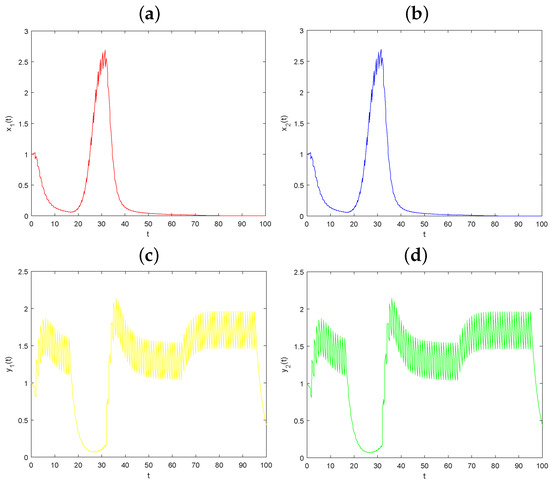
Figure 1. The global asymptotic stability from verification of the impulsive diffusion parameter D. System (1) with initial conditions $x_1\left(0\right)=1.0,y_1\left(0\right)=1.0,x_2\left(0\right)=1.0,y_2\left(0\right)=1.0$, as well as parameter values $a_1=0.7,b_1=0.2,a_2=0.7,b_2=0.2,{\beta }_1=0.5,{\beta }_2=0.5,k_1=0.5,k_2=0.5,{\mu }_1=0.5,$${\mu }_2=0.5,d_1=0.3,d_2=0.3,u=1,p=0.25,q=0.3,D=0.05,{\mu }_{11}=0.1,{\mu }_{12}=0.1,{\mu }_{21}=0.1$, and ${\mu }_{22}=0.1$, exhibits a globally asymptotically stable pest eradication periodic solution. The time-series of $x_1\left(t\right),x_2\left(t\right),y_1\left(t\right),y_2\left(t\right)$ are shown in (a–d), respectively.

It is evident that condition (26) is satisfied, indicating that system (1) is permanent (see Figure 2). By evaluating Equations (16) and (26), we can determine the existence of a threshold, denoted as $D^{*}$, which satisfies the following condition:

$$\underset{i=1,2}{max}\left\{a_{i}u-\frac{{\beta }_i}{d_i}\left[y_i^{*}(1-e^{-d_{i}pu})+y_i^{**}(1-e^{-d_{i}qu})+y_i^{***}(1-e^{-d_i(1-(p+q))u)})\right]\right\}<0(i=1,2)$$

or

$$\underset{i=1,2}{min}\left\{a_{i}u-\frac{{\beta }_i}{d_i}\left[y_i^{*}(1-e^{-d_{i}pu})+y_i^{**}(1-e^{-d_{i}qu})+y_i^{***}(1-e^{-d_i(1-(p+q)u)})\right]\right\}>0(i=1,2).$$

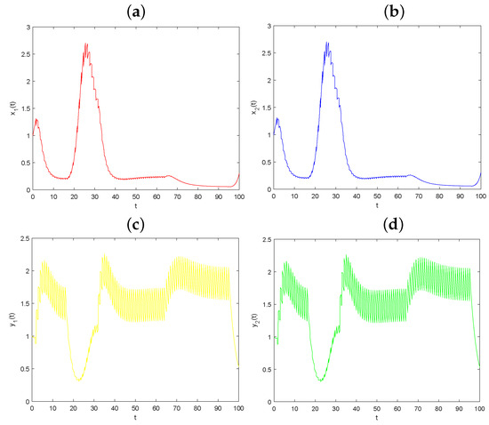
Figure 2. The permanence from verification of the impulsive diffusion parameter D. System (1) with initial conditions $x_1\left(0\right)=1.0$, $y_1\left(0\right)=1.0$, $x_2\left(0\right)=1.0$, $y_2\left(0\right)=1.0$, along with parameter values $a_1=0.9$, $b_1=0.2$, $a_2=09$, $b_2=0.2$, ${\beta }_1=0.5$, ${\beta }_2=0.5$, $k_1=0.5$, $k_2=0.5$, ${\mu }_1=0.5$, ${\mu }_2=0.5$, $d_1=0.3$, $d_2=0.3$, $u=1$, $p=0.25$, $q=0.3$, $D=0.95$, ${\mu }_{11}=0.1$, ${\mu }_{12}=0.1$, ${\mu }_{21}=0.1$, and ${\mu }_{22}=0.1$, satisfies the condition of permanence. The time-series of $x_1\left(t\right)$, $x_2\left(t\right)$, $y_1\left(t\right)$, and $y_2\left(t\right)$ are displayed in (a–d), respectively.

When the value of D is less than $D^{*}$, the pest populations will tend towards extinction. Conversely, if D is greater than $D^{*}$, the system will exhibit its permanence.

5.2. The Dynamical Behaviors Influenced by Parameters ${\mu }_1$ and ${\mu }_2$

In this subsection, we assume that $\mu ={\mu }_1={\mu }_2$. The initial values are set as $x_1\left(0\right)=1.0$, $y_1\left(0\right)=1.0$, $x_2\left(0\right)=1.0$, and $y_2\left(0\right)=1.0$. We consider various parameter values: $a_1=0.8$, $b_1=0.2$, $a_2=0.8$, $b_2=0.2$, and

${\beta }_1$	${\beta }_2$	$k_1$	$k_2$	${\mu }_1$	${\mu }_2$	$d_1$	$d_2$	u	p	q	D	${\mu }_{11}$	${\mu }_{12}$	${\mu }_{21}$	${\mu }_{22}$
0.5	0.5	0.5	0.5	0.5	0.5	0.3	0.3	1.0	0.25	0.3	0.4	0.1	0.1	0.1	0.1

It is obvious that conditions (15) and (16) are satisfied. Consequently, the periodic solution representing pest eradication in system (1) is globally asymptotically stable (see Figure 3). Similarly, assuming initial values $x_1\left(0\right)=1.0,y_1\left(0\right)=1.0,x_2\left(0\right)=1.0$, and $y_2\left(0\right)=1.0$, we set the following parameter values: $a_1=0.9,b_1=0.2,a_2=0.9,b_2=0.2$, and

${\beta }_1$	${\beta }_2$	$k_1$	$k_2$	${\mu }_1$	${\mu }_2$	$d_1$	$d_2$	u	p	q	D	${\mu }_{11}$	${\mu }_{12}$	${\mu }_{21}$	${\mu }_{22}$
0.5	0.5	0.5	0.5	0.1	0.1	0.3	0.3	1.0	0.25	0.3	0.2	0.1	0.1	0.1	0.1

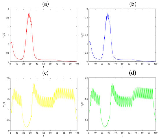
Figure 3. The global asymptotic stability from verification of the natural enemies release parameters ${\mu }_1$ and ${\mu }_2$. System (1) with initial conditions $x_1\left(0\right)=1.0$, $y_1\left(0\right)=1.0$, $x_2\left(0\right)=1.0$, $y_2\left(0\right)=1.0$, along with parameter values $a_1=0.8$, $b_1=0.2$, $a_2=0.8$, $b_2=0.2$, ${\beta }_1=0.5$, ${\beta }_2=0.5$, $k_1=0.5$, $k_2=0.5$, ${\mu }_1=0.5$, ${\mu }_2=0.5$, $d_1=0.3$, $d_2=0.3$, $u=1$, $p=0.25$, $q=0.3$, $D=0.4$, ${\mu }_{11}=0.1$, ${\mu }_{12}=0.1$, ${\mu }_{21}=0.1$, and ${\mu }_{22}=0.1$, exhibits a globally asymptotically stable pest eradication periodic solution. The time-series of $x_1\left(t\right)$, $x_2\left(t\right)$, $y_1\left(t\right)$, and $y_2\left(t\right)$ are displayed in (a–d), respectively.

It is apparent that condition (26) is satisfied, indicating that system (1) is permanent (see Figure 4). By analysis, we can establish the existence of a threshold value ${\mu }^{*}$. If $\mu$ is greater than ${\mu }^{*}$, the pest population will inevitably go extinct. Conversely, if $\mu$ is less than ${\mu }^{*}$, the system will exhibit its permanence.

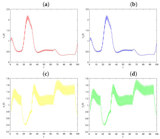
Figure 4. The permanence from verification of the natural enemies release parameters ${\mu }_1$ and ${\mu }_2$. System (1) exhibits permanence with initial conditions $x_1\left(0\right)=1.0$, $y_1\left(0\right)=1.0$, $x_2\left(0\right)=1.0$, $y_2\left(0\right)=1.0$, and parameters $a_1=0.9$, $b_1=0.2$, $a_2=0.9$, $b_2=0.2$, ${\beta }_1=0.5$, ${\beta }_2=0.5$, $k_1=0.5$, $k_2=0.5$, ${\mu }_1=0.1$, ${\mu }_2=0.1$, $d_1=0.3$, $d_2=0.3$, $u=1$, $p=0.25$, $q=0.3$, $D=0.2$, ${\mu }_{11}=0.1$, ${\mu }_{12}=0.1$, ${\mu }_{21}=0.1$, and ${\mu }_{22}=0.1$. The time-series of $x_1\left(t\right)$, $x_2\left(t\right)$, $y_1\left(t\right)$, and $y_2\left(t\right)$ are shown in (a–d), respectively.

5.3. The Dynamical Behaviors Influenced by Parameters ${\mu }_{ij}(i=1,2)$

In this subsection, we consider the scenario where all values of ${\mu }^{\prime },{\mu }_{11},{\mu }_{12},{\mu }_{21}$, and ${\mu }_{22}$ are equal. Initially, we set the following conditions for the pest management system: $x_1\left(0\right)=1.0,y_1\left(0\right)=1.0,x_2\left(0\right)=1.0$, $y_2\left(0\right)=1.0$. Furthermore, we assign parameter values as follows: $a_1=0.6,b_1=0.2,a_2=0.6,b_2=0.2$, and

${\beta }_1$	${\beta }_2$	$k_1$	$k_2$	${\mu }_1$	${\mu }_2$	$d_1$	$d_2$	u	p	q	D	${\mu }_{11}$	${\mu }_{12}$	${\mu }_{21}$	${\mu }_{22}$
0.5	0.5	0.5	0.5	0.35	0.35	0.3	0.3	1.0	0.25	0.5	0.2	0.3	0.3	0.3	0.3

It is confirmed that conditions (15) and (16) are satisfied, and the pest eradication periodic solution of system (1) is demonstrated to be globally asymptotically stable, as depicted in Figure 5. Subsequently, we maintain the same initial conditions as before but make adjustments to certain parameter values: $a_1=0.6,b_1=0.2,a_2=0.6,b_2=0.2$, and

${\beta }_1$	${\beta }_2$	$k_1$	$k_2$	${\mu }_1$	${\mu }_2$	$d_1$	$d_2$	u	p	q	D	${\mu }_{11}$	${\mu }_{12}$	${\mu }_{21}$	${\mu }_{22}$
0.5	0.5	0.5	0.5	0.35	0.35	0.3	0.3	1.0	0.25	0.5	0.2	0.05	0.05	0.05	0.05

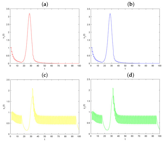
Figure 5. The global asymptotical stability from verification of the pesticide spraying parameters ${\mu }_{ij},i=1,2$. The periodic solution of system (1) with initial conditions $x_1\left(0\right)=1.0$, $y_1\left(0\right)=1.0$, $x_2\left(0\right)=1.0$, $y_2\left(0\right)=1.0$ is globally asymptotically stable for pest eradication with parameters $a_1=0.6$, $b_1=0.2$, $a_2=0.6$, $b_2=0.2$, ${\beta }_1=0.5$, ${\beta }_2=0.5$, $k_1=0.5$, $k_2=0.5$, ${\mu }_1=0.35$, ${\mu }_2=0.35$, $d_1=0.3$, $d_2=0.3$, $u=1$, $p=0.25$, $q=0.5$, $D=0.2$, ${\mu }_{11}=0.3$, ${\mu }_{12}=0.3$, ${\mu }_{21}=0.3$, and ${\mu }_{22}=0.3$. The time-series of $x_1\left(t\right)$, $x_2\left(t\right)$, $y_1\left(t\right)$, and $y_2\left(t\right)$ are shown in parts (a–d), respectively.

We verify that condition (26) is satisfied and observe that system (1) exhibits its permanence, as depicted in Figure 6. Through calculations, we determine the existence of a threshold value, denoted as ${\mu }^{**}$, if ${\mu }^{\prime }$ exceeds ${\mu }^{**}$, the pest population will become extinct. Conversely, if ${\mu }^{\prime }$ is lower than ${\mu }^{**}$, the system will exhibit its permanence.

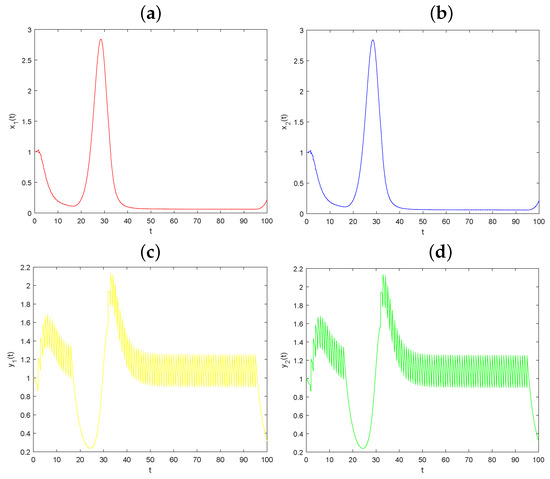
Figure 6. The permanence from verification of the pesticide spraying parameters ${\mu }_{ij},i=1,2$. System (1) exhibits permanence with initial conditions $x_1\left(0\right)=1.0$, $y_1\left(0\right)=1.0$, $x_2\left(0\right)=1.0$, $y_2\left(0\right)=1.0$, along with the following parameter values: $a_1=0.6$, $b_1=0.2$, $a_2=0.6$, $b_2=0.2$, ${\beta }_1=0.5$, ${\beta }_2=0.5$, $k_1=0.5$, $k_2=0.5$, ${\mu }_1=0.35$, ${\mu }_2=0.35$, $d_1=0.3$, $d_2=0.3$, $u=1$, $p=0.25$, $q=0.5$, $D=0.2$, ${\mu }_{11}=0.05$, ${\mu }_{12}=0.05$, ${\mu }_{21}=0.05$, and ${\mu }_{22}=0.05$. The time-series plots of $x_1\left(t\right)$, $x_2\left(t\right)$, $y_1\left(t\right)$, and $y_2\left(t\right)$ confirm the system’s permanence (a–d).

6. Conclusions

Based on our numerical simulations, we have found that increasing the diffusion has a negative impact on integrated pest management. However, we can achieve optimal pest control at a lower cost by implementing a combination of control strategies such as population dispersal, pesticide spraying, and natural enemies release. This study concludes that impulsive diffusion, pesticide spraying, and natural enemies release provide a solid foundation for effective pest management tactics.

References

- Tang, S.; Xiao, Y.; Chen, L.; Cheke, R.A. Integrated pest management models and their dynamical behaviour. Bull. Math. Biol. 2005, 31, 115–135. [Google Scholar] [CrossRef] [PubMed]
- Liang, J.; Tang, S.; Cheke, R.A. An integrated pest management model with delayed responses to pesticide applications and its threshold dynamics. Nonlinear Anal. Real World Appl. 2012, 13, 2352–2374. [Google Scholar] [CrossRef]
- Tang, S.; Tang, G.; Cheke, R.A. Optimum timing for integrated pest management: Modelling rates of pesticide application and natural enemy releases. J. Theor. Biol. 2010, 264, 623–638. [Google Scholar] [CrossRef] [PubMed]
- Liang, J.; Tang, S.; Cheke, R.A. Beverton-Holt discrete pest management models with pulsed chemical control and evolution of pesticide resistance. Commun. Nonlinear Sci. Numer. Simul. 2016, 36, 327–341. [Google Scholar] [CrossRef]
- Sun, K.; Zhang, T.; Tian, Y. Theoretical study and control optimization of an integrated pest management predator-prey model with power growth rate. Math. Biosci. 2016, 279, 13–26. [Google Scholar] [CrossRef] [PubMed]
- Akman, O.; Comar, T.; Henderson, M. An analysis of an impulsive stage structured integrated pest management model with refuge effect. Chaos Soliton Fract. 2018, 111, 44–54. [Google Scholar] [CrossRef]
- Sun, K.; Zhang, T.; Tian, Y. Dynamics analysis and control optimization of a pest management predator-prey model with an integrated control strategy. Appl. Math. Comput. 2017, 292, 253–271. [Google Scholar] [CrossRef]
- Akman, O.; Comar, T.D.; Hrozencik, D. Model selection for integrated pest management with stochasticity. J. Theor. Biol. 2018, 442, 110–122. [Google Scholar] [CrossRef] [PubMed]
- Chowdhury, J.; Al Basir, F.; Takeuchi, Y.; Ghosh, M.; Roy, P.K. A mathematical model for pest management in Jatropha curcas with integrated pesticides—An optimal control approach. Ecol. Complex. 2019, 37, 24–31. [Google Scholar] [CrossRef]
- Rezaei, R.; Safa, L.; Ganjkhanloo, M.M. Understanding farmers’ ecological conservation behavior regarding the use of integrated pest management—An application of the technology acceptance model. Glob. Ecol. Conserv. 2020, 22, e00941. [Google Scholar] [CrossRef]
- Li, W.; Chen, Y.; Huang, L.; Wang, J. Global dynamics of a filippov predator-prey model with two thresholds for integrated pest management. Chaos Soliton Fract. 2022, 157, 111881. [Google Scholar] [CrossRef]
- Liu, B.; Hu, G.; Kang, B.; Huang, X. Analysis of a hybrid pest management model incorporating pest resistance and different control strategies. Math. Biosci. Eng. 2020, 17, 4364–4383. [Google Scholar] [CrossRef] [PubMed]
- Liu, B.; Kang, B.; Tao, F.; Hu, G. Modelling the Effects of Pest Control with Development of Pesticide Resistance. Acta Math. Sin. Engl. 2021, 37, 109–125. [Google Scholar] [CrossRef]
- Liu, J.; Qi, Q.; Liu, B.; Gao, S. Pest control switching models with instantaneous and non-instantaneous impulsive effects. Math. Comput. Simul. 2023, 205, 926–938. [Google Scholar] [CrossRef]
- Jiao, J.; Chen, L.; Luo, G. An appropriate pest management SI model with biological and chemical control concern. Appl. Math. Comput. 2008, 196, 285–293. [Google Scholar] [CrossRef]
- Desneux, N.; Han, P.; Mansour, R.; Arnó, J.; Brévault, T.; Campos, M.R.; Chailleux, A.; Guedes, R.N.; Karimi, J.; Konan, K.A.J.; et al. Integrated pest management of Tuta absoluta: Practical implementations across different world regions. J. Pest Sci. 2022, 95, 17–39. [Google Scholar] [CrossRef]
- Golan, K.; Kot, I.; Kmieć, K.; Górska-Drabik, E. Approaches to Integrated Pest Management in Orchards: Comstockaspis perniciosa (Comstock) Case Study. Agriculture 2023, 13, 131. [Google Scholar] [CrossRef]
- Zhou, A.; Sattayatham, P.; Jiao, J. Analysis of a predator-prey model with impulsive diffusion and releasing on predator population. Adv. Differ. Equ. 2016, 2016, 111. [Google Scholar] [CrossRef]
- Murray, J.D. Mathematical Biology; Springer: Berlin/Heidelberg, Germany; New York, NY, USA, 1989. [Google Scholar]
- Tang, S.; Xiao, Y.; Liang, J.; Wang, X. Mathematical Biology; Science Press: Beijing, China, 2019. (In Chinese) [Google Scholar]
- Jury, E.L. Inners and Stability of Dynamics System; Wiley: New York, NY, USA, 1974. [Google Scholar]
- Bainov, D.; Simeonov, P. Impulsive Differential Equations: Periodic Solution and Applications, Longman Scientific and Technical; CRC Press: New York, NY, USA, 1993. [Google Scholar]
- Lakshmikantham, V.; Bainov, D.; Simeonov, P. Theory of Impulsive Differential Equations; World Scientific: Singapore, 1989. [Google Scholar]
Disclaimer/Publisher’s Note: The statements, opinions and data contained in all publications are solely those of the individual author(s) and contributor(s) and not of MDPI and/or the editor(s). MDPI and/or the editor(s) disclaim responsibility for any injury to people or property resulting from any ideas, methods, instructions or products referred to in the content. |
© 2023 by the author. Licensee MDPI, Basel, Switzerland. This article is an open access article distributed under the terms and conditions of the Creative Commons Attribution (CC BY) license (https://creativecommons.org/licenses/by/4.0/).