Bayesian Subset Selection of Seasonal Autoregressive Models

Abstract

Seasonal autoregressive (SAR) models have many applications in different fields, such as economics and finance. It is well known in the literature that these models are nonlinear in their coefficients and that their Bayesian analysis is complicated. Accordingly, choosing the best subset of these models is a challenging task. Therefore, in this paper, we tackled this problem by introducing a Bayesian method for selecting the most promising subset of the SAR models. In particular, we introduced latent variables for the SAR model lags, assumed model errors to be normally distributed, and adopted and modified the stochastic search variable selection (SSVS) procedure for the SAR models. Thus, we derived full conditional posterior distributions of the SAR model parameters in the closed form, and we then introduced the Gibbs sampler, along with SSVS, to present an efficient algorithm for the Bayesian subset selection of the SAR models. In this work, we employed mixture–normal, inverse gamma, and Bernoulli priors for the SAR model coefficients, variance, and latent variables, respectively. Moreover, we introduced a simulation study and a real-world application to evaluate the accuracy of the proposed algorithm.

1. Introduction

Seasonal autoregressive (SAR) time series models are widely used in different fields such as economics and finance to fit and forecast time series that are characterized by seasonality [1]. As it is well known, time series modeling starts with the specification of the model order, followed by estimation, diagnostic checks, and forecasting [2]. Therefore, the model specification phase is important, since all other modeling phases depend on its accuracy. In most real-world applications, the number of time series lags incorporated in a proposed time series model for an underlying time series is unknown, and this number of time series lags in this case is known as the model order, which needs to be specified or estimated based on the given time series data and its assumed probability distribution [3].

Although the time series model order is usually unknown, a maximum value of this order can be assumed, and different methods can be introduced to select the best subset to have a parsimonious model. Traditional subset selection methods include information criteria, such as the Akaike information criterion (AIC) [4] and the corrected AIC (AIC${}_c$) [5]. These traditional selection methods use exhaustive searches based on parameter estimation and order selection. Many researchers have used these methods for subset selection in autoregressive (AR) time series models, including McClave [6], Penm and Terrell [7], Thanoon [8], Sarkar and Kanjilal [9].

However, it is very computationally expensive to apply these traditional methods to complicated models with high orders, such as the SAR models and other time series models with multiple seasonalities [10,11]. Accordingly, other subset selection procedures based on Markov chain Monte Carlo (MCMC) methods have been proposed for reducing the computational cost and efficiently selecting the best subset of time series models. Some researchers have adopted the stochastic search variable selection (SSVS) procedure, which was introduced by George and McCulloch [12], for selecting the best subset of linear regression models to be applied to the subset selection of time series models. Chen [13] proposed the Gibbs sampler, along with the SSVS procedure, to select the best subset of AR models. This work has been extended by different researchers to other time series models. So et al. [14] extended it for the subset selection of AR models with exogenous variables, and Chen et al. [15] extended it for the subset selection of threshold ARMA models.

On the other hand, the Bayesian analysis of the SAR model is complicated, because the likelihood function is a nonlinear function of the SAR model coefficients, and, accordingly, its posterior density is analytically intractable. Different approaches have been introduced to facilitate this analysis, including Markov chain Monte Carlo (MCMC)-based approximations [16]. Barnett et al. [17,18] applied MCMC methods to estimate SAR and ARMA models based on sampling functions for partial autocorrelations. Ismail [19,20] applied the Gibbs sampler to introduce the Bayesian analysis of SAR and SMA models. Ismail and Amin [16] applied the Gibbs sampler to present the Bayesian estimation of seasonal ARMA (SARMA) models, and, recently, Amin [1] used the same approach to introduce the Bayesian prediction of SARMA models. For modeling time series with multiple seasonalities, Amin and Ismail [21] and Amin [22,23] applied the Gibbs sampler to introduce the Bayesian estimation of double SAR, SMA, and SARMA models. Recently, Amin [24,25] applied the Gibbs sampler to introduce the Bayesian analysis of double and triple SAR models.

From a real-world application perspective, it is crucial to introduce an efficient Bayesian method for selecting the best subset of the SAR models, with the aim to obtain a parsimonious SAR model. However, most of the existing work has focused only on the Bayesian estimation and the prediction of SAR processes, and none of them has tried to tackle this problem of selecting the best subset of the SAR models. Therefore, in this paper, we aim to fill this gap and enrich real-world applications of the SAR models by introducing a Bayesian method for subset selection of these models based on modifying the SSVS procedure and adopting the Gibbs sampler. In particular, we first introduce latent variables for the nonseasonal and seasonal SAR model lags, assume that the SAR model errors are normally distributed, and employ mixture–normal, inverse gamma, and Bernoulli priors for the SAR model coefficients, variance, and latent variables, respectively. We then derive full conditional posteriors of the SAR model parameters in the closed form, and we apply the Gibbs sampler, along with SSVS, to develop an efficient algorithm for the best subset selection of the SAR models. In order to evaluate the performance of the proposed algorithm, we conduct a simulation study and a real-world application.

The remainder of this paper is organized as follows: We summarize the SAR models and related Bayesian concepts in Section 2. We then introduce the posterior analysis and proposed algorithm for the Bayesian best subset selection of the SAR models in Section 3. In Section 4, we present and discuss simulations and the real-world application of the proposed Bayesian subset selection algorithm. Finally, we conclude this work in Section 5.

2. Seasonal Autoregressive (SAR) Models and Bayesian Concepts

A mean deleted time series $\left\{z_t\right\}$ is generated by a seasonal autoregressive model of order $p_1$ and $p_2$, and is designated as SAR$\left(p_1\right){\left(p_2\right)}_s$ if it satisfies [2]:

$$\begin{array}{c}\hfill {\mathit{\varphi }}_{\mathbf{1}}\left(B\right){\mathit{\varphi }}_{\mathbf{2}}\left(B^s\right)z_t={\epsilon }_t,\end{array}$$

(1)

where the SAR errors $\left\{{\epsilon }_t\right\}$ are assumed to follow a normal distribution with a mean zero and variance of ${\sigma }^2$, s is the seasonal period, and B is an operator defined as $B^r{z}_t=z_{t-r}$. ${\mathit{\varphi }}_{\mathbf{1}}\left(B\right)=\left(1-{\varphi }_{11}B-{\varphi }_{12}{B}^2-\dots -{\varphi }_{1p_1}{B}^{p_1}\right)$ and ${\mathit{\varphi }}_{\mathbf{2}}\left(B^s\right)=\left(1-{\varphi }_{21}{B}^s-{\varphi }_{22}{B}^{2s}-\dots -{\varphi }_{2p_2}{B}^{p_{2}s}\right)$ are the nonseasonal and seasonal autoregressive polynomials with orders $p_1$ and $p_2$, respectively. Also, ${\mathit{\varphi }}_{\mathbf{1}}={\left({\varphi }_{11},{\varphi }_{12},\dots ,{\varphi }_{1p_1}\right)}^T$ and ${\mathit{\varphi }}_{\mathbf{2}}={\left({\varphi }_{21},{\varphi }_{22},\dots ,{\varphi }_{2p_2}\right)}^T$ are the nonseasonal and seasonal autoregressive coefficients, respectively.

We can expand the SAR model (1) and write it as follows:

$$\begin{array}{c}\hfill z_t=\sum _{i=1}^{p_1}{\varphi }_{1i}{z}_{t-i}+\sum _{j=1}^{p_2}{\varphi }_{2j}{z}_{t-js}-\sum _{i=1}^{p_1}\sum _{j=1}^{p_2}{\varphi }_{1i}{\varphi }_{2j}{z}_{t-i-js}+{\epsilon }_t.\end{array}$$

(2)

With the objective of simplifying the Bayesian analysis, we write the SAR model (2) in a matrix notation as follows:

$$\begin{array}{c}\hfill \mathit{y}=\mathit{X}\mathit{\beta }+\mathit{E},\end{array}$$

(3)

where $\mathit{y}={\left(z_1,z_2,\dots ,z_n\right)}^T$, $\mathit{E}={\left({\epsilon }_1,{\epsilon }_2,\cdots ,{\epsilon }_n\right)}^T$, and $\mathit{X}$ is an $n\times m$ matrix, i.e., $m=(1+p_1)(1+p_2)-1$, with the $t^{th}$ row defined as:

$$\begin{array}{c}\hfill X_t=\left(z_{t-1},\cdots ,z_{t-p_1},z_{t-s},z_{t-s-1},\cdots ,z_{t-s-p_1},\cdots \cdots ,z_{t-p_{2}s},z_{t-p_{2}s-1},\cdots ,z_{t-p_{2}s-p_1}\right),\end{array}$$

(4)

and $\mathit{\beta }$ is the coefficient vector, which is defined as the following:

$$\begin{array}{c}\hfill \mathit{\beta }={\left({\varphi }_{11},\cdots ,{\varphi }_{1p_1},{\varphi }_{21},-{\varphi }_{11}{\varphi }_{21},\cdots ,-{\varphi }_{1p_1}{\varphi }_{21},\cdots \cdots ,{\varphi }_{2p_2},-{\varphi }_{11}{\varphi }_{2p_2},\cdots ,-{\varphi }_{1p_1}{\varphi }_{2p_2}\right)}^T.\end{array}$$

(5)

The products of the coefficients, i.e., ${\varphi }_{1i}{\varphi }_{2j}^{\prime }s$, are part of the SAR model, and, accordingly, this model is a nonlinear function of ${\mathit{\varphi }}_{\mathbf{1}}$ and ${\mathit{\varphi }}_{\mathbf{2}}$, thereby leading to complications in its Bayesian analysis.

As we mentioned in the introduction, one of the main challenges of time series analysis is specifying the value of the SAR model order $p_1$ and $p_2$, since these values are unknown and depend on the stochastic structure of the time series under study. Thus, we assume that the maximum value of the SAR model order is known, and we adopt and modify the SSVS procedure for the Bayesian best subset selection of the SAR model. Accordingly, we first introduce a latent variable for each coefficient of the SAR model, i.e., ${\delta }_{ij}$ for ${\varphi }_{ij}$$\forall j=1,\dots ,p_i\mathrm{and}i=1,2$, where ${\delta }_{ij}$ equals to one when the corresponding time series lag to ${\varphi }_{ij}$ is selected, and it equals to zero otherwise. We then represent the prior distribution on each SAR model coefficient ${\varphi }_{ij}$ using a mixture–normal distribution that is defined as:

$$\begin{array}{c}\hfill {\varphi }_{ij}|{\delta }_{ij}\sim (1-{\delta }_{ij})N(0,{\tau }_{ij}^2)+{\delta }_{ij}N(0,c_{ij}^2{\tau }_{ij}^2),\end{array}$$

(6)

and

$$\begin{array}{c}\hfill p({\delta }_{ij}=1)=1-p({\delta }_{ij}=0)=P_{ij}\forall ij.\end{array}$$

(7)

Thus, the prior distribution of ${\mathit{\varphi }}_{\mathbf{1}}$ and ${\mathit{\varphi }}_{\mathbf{2}}$ can be presented as a multivariate normal distribution that is defined as follows:

$$\begin{array}{c}\hfill {\mathit{\varphi }}_{\mathit{i}}|{\mathit{\delta }}_{\mathit{i}}\sim N_{p_i}(\mathbf{0},M_{{\delta }_i}{W}_i{M}_{{\delta }_i})\forall i=1,2,\end{array}$$

(8)

where ${\mathit{\delta }}_{\mathit{i}}={({\delta }_{i1},\cdots ,{\delta }_{i{p}_i})}^T$, $M_{{\delta }_i}$ is a diagonal matrix, i.e., $M_{{\delta }_i}=diag[b_{i1}{\tau }_{i1},\cdots ,b_{i{p}_i}{\tau }_{i{p}_i}]$ with $b_{ij}=1$ if ${\delta }_{ij}=0$ and $b_{ij}=c_{ij}$ if ${\delta }_{ij}=1$, and $W_i$ is a prior correlation matrix. Here, $M_{{\delta }_i}$ is specified in such a way to be a scaling of the prior covariance matrix to satisfy the prior specification in (6). In particular, we chose ${\tau }_{i1},\cdots ,{\tau }_{i{p}_i}$ to be small, and, therefore, the ${\varphi }_{ij}$s associated with ${\delta }_{ij}=0$ would likely be close to zero. In addition, we chose $c_{i1},\cdots ,c_{i{p}_i}$ to be large enough to make $c_{ij}^2{\tau }_{ij}^2$ highly greater than ${\tau }_{ij}^2$; thus, the ${\varphi }_{ij}$ associated with ${\delta }_{ij}=1$ would tend to have a high variation and likely be away from zero, and the corresponding time series lags were selected as the best subset SAR model. For more information about setting these constants in the SSVS procedure, we refer to George and McCulloch [12].

As a prior distribution of ${\sigma }^2$, we specify an inverse gamma distribution that is defined as:

$$\begin{array}{c}\hfill {\sigma }^2|{\mathit{\delta }}_{\mathit{i}}\sim IG\left(\frac{\nu }{2},\frac{\nu \lambda }{2}\right).\end{array}$$

(9)

Using the marginal distribution of the ${\delta }_{ij}$s given in (7), we can write the joint prior distribution of ${\mathit{\delta }}_{\mathit{i}}$ as:

$$\begin{array}{c}\hfill \zeta \left({\mathit{\delta }}_{\mathit{i}}\right)=\prod _{j=1}^{p_i}{P}_{ij}^{{\delta }_{i}j}{(1-P_{ij})}^{(1-{\delta }_{ij})}\forall i=1,2.\end{array}$$

(10)

It is worth noting that the uniform prior of ${\mathit{\delta }}_{\mathit{i}}$, i.e., $\zeta \left({\mathit{\delta }}_{\mathit{i}}\right)=2^{-p{}_i}\forall i=1,2$, is a special case, since each time series lag has the same probability to be selected.

The likelihood function of the SAR model (3) with normally distributed errors can be presented as:

$$\begin{array}{cc}\hfill L({\mathit{\varphi }}_{\mathbf{1}},{\mathit{\varphi }}_{\mathbf{2}},{\sigma }^2\mid \mathbf{y})& \hfill \propto {\left({\sigma }^2\right)}^{-\frac{n}{2}}exp\left\{-\frac{1}{2{\sigma }^2}{\mathit{E}}^T\mathit{E}\right\}\hfill \\ \hfill & \hfill ={\left({\sigma }^2\right)}^{-\frac{n}{2}}exp\left\{-\frac{1}{2{\sigma }^2}{\left(\mathit{y}-\mathit{X}\mathit{\beta }\right)}^T\left(\mathit{y}-\mathit{X}\mathit{\beta }\right)\right\}.\hfill \end{array}$$

(11)

We can obtain the joint posterior distribution of the SAR models by simply multiplying the prior distributions given in (8)–(10) by the likelihood function given in (11), which can be presented as:

$$\begin{array}{cc}\hfill \zeta \left({\mathit{\varphi }}_{\mathbf{1}},{\mathit{\varphi }}_{\mathbf{2}},{\sigma }^2,{\mathit{\delta }}_{\mathbf{1}},{\mathit{\delta }}_{\mathbf{2}}\mid \mathit{y}\right)& \hfill \propto \prod _{i=1}^2\prod _{j=1}^{p_i}{P}_{ij}^{{\delta }_{i}j}{(1-P_{ij})}^{(1-{\delta }_{ij})}{\left({\sigma }^2\right)}^{-\left(\frac{n+\nu }{2}+1\right)}\times \hfill \\ & \hfill exp\left\{-\frac{1}{2{\sigma }^2}\left[\nu \lambda +{\sigma }^2\sum _{i=1}^2{{\mathit{\varphi }}_{\mathit{i}}}^T\left(M_{{\delta }_i}{W}_i{M}_{{\delta }_i}\right){\mathit{\varphi }}_{\mathit{i}}+\right.\right.\hfill \\ & \hfill \left.\left.{\left(\mathit{y}-\mathit{X}\mathit{\beta }\right)}^T\left(\mathit{y}-\mathit{X}\mathit{\beta }\right)\right]\right\}.\hfill \end{array}$$

(12)

3. Bayesian Subset Selection of the SAR Models

The introduction of the Bayesian subset selection of the SAR models is based on posterior analysis; however, the joint posterior (12) of the SAR model parameters is a nonlinear function of the coefficients ${\mathit{\varphi }}_{\mathbf{1}}$ and ${\mathit{\varphi }}_{\mathbf{2}}$. Accordingly, this joint posterior is analytically intractable, and, thus, the marginal posterior of each parameter cannot be analytically derived in closed forms. One of the solutions that can be applied to tackle this problem and ease the Bayesian subset selection of the SAR models is introducing the Gibbs sampler to approximate the required marginal posteriors of these models. In this section, we first derive the conditional posterior distributions of the SAR model as a requirement to employ the Gibbs sampler, and we then introduce our proposed algorithm for the Bayesian subset selection of the SAR models.

3.1. Conditional Posteriors of the SAR Models

As we introduced in our previous work [1,10], deriving the conditional posterior of each SAR model parameter can be simply done from the joint posterior (12) by first combining related terms to that parameter and then integrating out all unrelated terms. Following the same approach, we derive here the full conditional posteriors of the SAR parameters, i.e., ${\mathit{\varphi }}_{\mathbf{1}}$, ${\mathit{\varphi }}_{\mathbf{2}}$, ${\sigma }^2,{\mathit{\delta }}_{\mathbf{1}}$, and ${\mathit{\delta }}_{\mathbf{2}}$, that are required to adopt the Gibbs sampler, along with SSVS for selecting the best subset of the SAR models.

We rewrite the SAR model (3) as the following:

$$\begin{array}{c}\hfill \mathit{y}=Z_{{\mathit{\varphi }}_{\mathbf{1}}}{\mathit{\varphi }}_{\mathbf{1}}+L_{{\mathit{\varphi }}_{\mathbf{1}}}{\mathit{\varphi }}_{\mathbf{2}}+\mathit{E}.\end{array}$$

(13)

We substitute (13) in the joint posterior (12), and we then complete the square in the exponent with respect to ${\mathit{\varphi }}_{\mathbf{1}}$ and integrate out all unrelated terms to obtain the conditional posterior of ${\mathit{\varphi }}_{\mathbf{1}}$ given ${\mathit{\varphi }}_{\mathbf{2}}$, ${\sigma }^2,{\mathit{\delta }}_{\mathbf{1}},{\mathit{\delta }}_{\mathbf{2}}$, and $\mathit{y}$ to be $N_{p_1}({\mu }_{{\varphi }_1}^{★},V_{{\varphi }_1}^{★})$, where:

$$\begin{array}{cc}\hfill {\mu }_{{\varphi }_1}^{★}& \hfill =\left[{\left({\sigma }^{-2}{Z}_{{\varphi }_1}^T{Z}_{{\varphi }_1}+{\left(M_{{\delta }_1}{W}_1{M}_{{\delta }_1}\right)}^{-1}\right)}^{-1}\left({\sigma }^{-2}{Z}_{{\varphi }_1}^T\left(\mathit{y}-L_{{\varphi }_1}{\mathit{\varphi }}_{\mathbf{2}}\right)\right)\right],\mathrm{and}\hfill \\ \hfill V_{{\varphi }_1}^{★}& ={\left({\sigma }^{-2}{Z}_{{\varphi }_1}^T{Z}_{{\varphi }_1}+{\left(M_{{\delta }_1}{W}_1{M}_{{\delta }_1}\right)}^{-1}\right)}^{-1},\hfill \end{array}$$

(14)

where $Z_{{\varphi }_1}$ is a $n\times p_1$ matrix with the $(t,i)$ element $Z_{{\varphi }_{1_{ti}}}=z_{t-i}-{\sum }_{j=1}^{p_2}{\varphi }_{2j}{z}_{t-i-js}$, and $L_{{\varphi }_1}$ is a $n\times p_2$ matrix with the $t^{th}$ row $L_{{\varphi }_{1_t}}=\left(z_{t-s},z_{t-2s},\cdots ,z_{t-p_{2}s}\right)$.

In the same way, we rewrite the SAR model (3) as the following:

$$\begin{array}{c}\hfill \mathbf{y}=Z_{{\mathit{\varphi }}_{\mathbf{2}}}{\mathit{\varphi }}_{\mathbf{2}}+L_{{\mathit{\varphi }}_{\mathbf{2}}}{\mathit{\varphi }}_{\mathbf{1}}+\mathit{E}.\end{array}$$

(15)

We substitute (15) in the joint posterior (12), and we then complete the square in the exponent with respect to ${\mathit{\varphi }}_{\mathbf{2}}$ and integrate out all unrelated terms to obtain the conditional posterior of ${\mathit{\varphi }}_{\mathbf{2}}$ given ${\mathit{\varphi }}_{\mathbf{1}},{\sigma }^2,{\mathit{\delta }}_{\mathbf{1}},{\mathit{\delta }}_{\mathbf{2}}$, and $\mathit{y}$ to be $N_{p_2}({\mu }_{{\varphi }_2}^{★},V_{{\varphi }_2}^{★})$, where:

$$\begin{array}{cc}\hfill {\mu }_{{\varphi }_2}^{★}& \hfill =\left[{\left({\sigma }^{-2}{Z}_{{\varphi }_2}^T{Z}_{{\varphi }_2}+{\left(M_{{\delta }_2}{W}_2{M}_{{\delta }_2}\right)}^{-1}\right)}^{-1}\left({\sigma }^{-2}{Z}_{{\varphi }_2}^T\left(\mathit{y}-L_{{\varphi }_2}{\mathit{\varphi }}_{\mathbf{1}}\right)\right)\right],\mathrm{and}\hfill \\ \hfill V_{{\varphi }_2}^{★}& ={\left({\sigma }^{-2}{Z}_{{\varphi }_2}^T{Z}_{{\varphi }_2}+{\left(M_{{\delta }_2}{W}_2{M}_{{\delta }_2}\right)}^{-1}\right)}^{-1},\hfill \end{array}$$

(16)

where $Z_{{\varphi }_2}$ is an $n\times p_2$ matrix with the $(t,j)$ element $Z_{{\varphi }_{2_{tj}}}=z_{t-js}-{\sum }_{i=1}^{p_1}{\varphi }_{1i}{z}_{t-i}$, and L${}_{{\varphi }_2}$ is an $n\times p_1$ matrix with the $t^{th}$ row $L_{{\varphi }_{2_t}}=\left(z_{t-1},z_{t-2},\cdots ,z_{t-p_1}\right)$.

Moreover, from the joint posterior (12), we easily derive the conditional posterior of ${\sigma }^2$ given ${\mathit{\varphi }}_{\mathbf{1}},{\mathit{\varphi }}_{\mathbf{2}},{\mathit{\delta }}_{\mathbf{1}},{\mathit{\delta }}_{\mathbf{2}}$, and $\mathit{y}$ to be an inverse gamma $IG(\frac{n+\nu }{2},\frac{{\lambda }^{★}}{2})$, where ${\lambda }^{★}=\nu \lambda +{\left(\mathit{y}-\mathit{X}\mathit{\beta }\right)}^T\left(\mathit{y}-\mathit{X}\mathit{\beta }\right)$.

Now, in order to simplify the deriving conditional posteriors of latent variables, we need to first simplify the notations. In particular, for the $j^{th}$ latent variable in the $i^{th}$ vector, we refer to other latent variables as ${\delta }_{i(-j)}$$\forall j=1,\dots ,p_i,\mathrm{and}i=1,2$. In addition, for the $i^{th}$ latent variable vector, we refer to other latent variable vectors as ${\mathit{\delta }}_{(-\mathit{i})}$. Accordingly, we derive the conditional posterior of each latent variable ${\delta }_{ij}$ given ${\mathit{\varphi }}_{\mathbf{1}},{\mathit{\varphi }}_{\mathbf{2}}$, ${\sigma }^2$, ${\delta }_{i(-j)}$, ${\mathit{\delta }}_{(-\mathit{i})}$, and $\mathit{y}$ to be a Bernoulli distribution with a probability that is defined as follows:

$$\begin{array}{c}\hfill p({\delta }_{ij}=1\mid {\mathit{\varphi }}_{\mathbf{1}},{\mathit{\varphi }}_{\mathbf{2}},{\sigma }^2,{\delta }_{i(-j)},{\mathit{\delta }}_{(-\mathit{i})},\mathit{y})=\frac{a_{ij}}{a_{ij}+b_{ij}}\forall ij,\end{array}$$

(17)

where $a_{ij}=P_{ij}\times \zeta ({\mathit{\varphi }}_{\mathit{i}}\mid {\mathit{\varphi }}_{(-\mathit{i})},{\sigma }^2,{\delta }_{i(-j)},{\mathit{\delta }}_{(-\mathit{i})},\mathit{y},{\delta }_{ij}=1)$, and $b_{ij}=(1-P_{ij})\times \zeta ({\mathit{\varphi }}_{\mathit{i}}\mid {\mathit{\varphi }}_{(-\mathit{i})},{\sigma }^2,{\delta }_{i(-j)},{\mathit{\delta }}_{(-\mathit{i})},\mathit{y},{\delta }_{ij}=0)$.

3.2. Proposed Algorithm for Bayesian Subset Selection of the SAR Models

Based on the work of the previous subsection, the required conditional posteriors of the SAR parameters are available, and we are accordingly able to adopt the SSVS and Gibbs sampler to propose an algorithm for the Bayesian subset selection of the SAR models.

We can implement our proposed algorithm for the Bayesian subset selection of the SAR models in the following steps:

1.

Set a maximum value for the SAR model order as ($p_1$, $p_2$).

2.

Apply the OLS method to estimate the SAR($p_1$)($p_2$)${}_s$ model, and set these estimates as initial values for the Gibbs Sampler—$\{{\mathit{\varphi }}_{\mathbf{1}}^{\mathbf{0}},{\mathit{\varphi }}_{\mathbf{2}}^{\mathbf{0}},{\left({\sigma }^2\right)}^0,{\mathit{\delta }}_{\mathbf{1}}^{\mathbf{0}},{\mathit{\delta }}_{\mathbf{2}}^{\mathbf{0}}\}$.

3.

Set the Gibbs sampler simulation design, which includes the number of simulations, burn-in, and thinning.

4.

Set r as the current simulation and simulate the conditional posteriors as the following:

• ${\delta }_{1j}^r\sim \zeta \left({\delta }_{1j}^r\mid \mathbf{y},{\mathit{\varphi }}_{\mathbf{1}}^{\mathit{r}-\mathbf{1}},{\mathit{\varphi }}_{\mathbf{2}}^{\mathit{r}-\mathbf{1}},{\left({\sigma }^2\right)}^r,{\delta }_{1(-j)}^r,{\mathit{\delta }}_{\mathbf{2}}^{\mathit{r}}\right)=Bin\left(1,\frac{a_{1j}}{a_{1j}+b_{1j}}\right)$, $\forall j=1,\dots ,p_1$.
• ${\delta }_{2j}^r\sim \zeta \left({\delta }_{2j}^r\mid \mathbf{y},{\mathit{\varphi }}_{\mathbf{1}}^{\mathit{r}-\mathbf{1}},{\mathit{\varphi }}_{\mathbf{2}}^{\mathit{r}-\mathbf{1}},{\left({\sigma }^2\right)}^r,{\delta }_{2(-j)}^r,{\mathit{\delta }}_{\mathbf{1}}^{\mathit{r}}\right)=Bin\left(1,\frac{a_{2j}}{a_{2j}+b_{2j}}\right)$, $\forall j=1,\dots ,p_2$.
• ${\mathit{\varphi }}_{\mathbf{1}}^{\mathit{r}}\sim \zeta \left({\mathit{\varphi }}_{\mathbf{1}}^{\mathit{r}}\mid \mathbf{y},{\mathit{\varphi }}_{\mathbf{2}}^{\mathit{r}-\mathbf{1}},{\left({\sigma }^2\right)}^{r-1},{\mathit{\delta }}_{\mathbf{1}}^{\mathit{r}},{\mathit{\delta }}_{\mathbf{2}}^{\mathit{r}}\right)=N({\mu }_{{\varphi }_1}^{★},V_{{\varphi }_1}^{★}),$
• ${\mathit{\varphi }}_{\mathbf{2}}^{\mathit{r}}\sim \zeta \left({\mathit{\varphi }}_{\mathbf{2}}^{\mathit{r}}\mid \mathbf{y},{\mathit{\varphi }}_{\mathbf{1}}^{\mathit{r}},{\left({\sigma }^2\right)}^{r-1},{\mathit{\delta }}_{\mathbf{1}}^{\mathit{r}},{\mathit{\delta }}_{\mathbf{2}}^{\mathit{r}}\right)=N({\mu }_{{\varphi }_2}^{★},V_{{\varphi }_2}^{★}),$
• ${\left({\sigma }^2\right)}^r\sim \zeta \left({\left({\sigma }^2\right)}^r\mid \mathbf{y},{\mathit{\varphi }}_{\mathbf{1}}^{\mathit{r}},{\mathit{\varphi }}_{\mathbf{2}}^{\mathit{r}},{\mathit{\delta }}_{\mathbf{1}}^{\mathit{r}},{\mathit{\delta }}_{\mathbf{2}}^{\mathit{r}}\right)=IG\left(\frac{n+{\nu }^{★}}{2},\frac{{\lambda }^{★}}{2}\right).$

In this $r^{th}$ simulation, the generated values together construct the $r^{th}$ value of the Markov chain, i.e., $\{{\mathit{\varphi }}_{\mathbf{1}}^{\mathit{r}},{\mathit{\varphi }}_{\mathbf{2}}^{\mathit{r}},{\left({\sigma }^2\right)}^r,{\mathit{\delta }}_{\mathbf{1}}^{\mathit{r}},{\mathit{\delta }}_{\mathbf{2}}^{\mathit{r}}\}$.

5.

Repeat step (4) until all the required Gibbs sampler simulations have been conducted.

6.

Apply the burn-in and thinning processes for the simulated Markov chain and monitor the convergence using autocorrelations, Raftery and Lewis diagnostics [26], and Geweke diagnostics [27]. For more information about these convergence diagnostics, see LeSage [28] and Amin [1,10].

7.

Once the convergence of the simulated Markov chain is confirmed, select the best SAR subset that corresponds to a value of latent variables with the highest frequency in the simulated Markov chain, and also (whenever it is needed) compute the Bayesian estimates of the SAR parameters directly using the sample averages of these simulation outputs.

4. Simulations and Real Application

In this section, we introduce a simulation study and a real-world application for the proposed Bayesian algorithm for selecting the best subset selection for the SAR models, wherein we aim to evaluate its accuracy and applicability.

4.1. Simulation Study

We performed simulations from four SAR models using a simulation design that is presented in Table 1. The parameters of these SAR models were selected to cover different seasonality patterns, without any bias to select specific models or parameters. In particular, the first two SAR models are examples of SAR(2)(1)${}_{12}$, the third SAR model is an example of SAR(1)(2)${}_{12}$, and the fourth SAR model is an example of SAR(2)(2)${}_{12}$.

Table 1. Simulation design.

Model	${\mathit{\varphi }}_{11}$	${\mathit{\varphi }}_{12}$	${\mathit{\varphi }}_{21}$	${\mathit{\varphi }}_{22}$	s	${\mathit{\sigma }}^2$
I	0.5	0.3	0.4	-	12	1.0
II	1.5	−0.9	0.6	-	12	1.0
III	0.6	-	0.5	0.4	12	1.0
IV	1.5	−0.9	0.5	0.4	12	1.0

We first generated 1,000 time series from each SAR model with different sizes, from 100 to 500 with an increment of 100, and we then applied the proposed Bayesian algorithm for selecting the best subset of the SAR model, as described in Section 3.2.

We set the Gibbs sampler simulation design as follows:

The number of Gibbs sampler simulations equaled 11,000, the burn-in equaled 1000, and thinning level equaled 10. In addition, we set the maximum order value of the SAR model (2) to be three, i.e., $p_i=5\forall i=1,2$. Using Gibbs sampler draws, we computed the frequency values for each latent variable to find the best subset of the SAR model as a value with the highest frequency. Also, whenever it is needed, we can easily compute Bayesian estimates of the SAR model parameters as the following summary statistics: mean, standard deviation, and ($2.5^{th}$, $97.5^{th}$) percentiles of draws as a 95% credible interval. We evaluated the accuracy of our proposed Bayesian algorithm for the best subset selection of the SAR models by simply computing the percentage of correctly selected best subset SAR models. In addition, for the sake of comparison, we used the traditional subset selection methods, including the AIC and AIC${}_c$, to select the best subset of the simulated SAR models and also computed their percentage of correctly selected best subset SAR models. We can illustrate in some detail how our proposed algorithm works for the best subset selection of the SAR models by presenting all the results of the Gibbs sampler draws for only one time series of size $n=300$ generated from Model I. For this generated time series, we display the Bayesian subset selection results in Table 2 and the estimation results in Table 3.

Table 2. Bayesian subset selection results for one time series generated from Model I.

Non-Seasonal Latent Variables			Seasonal Latent Variables
${\mathit{\delta }}_{\mathbf{1}}$	Freq	Percent	${\mathit{\delta }}_{\mathbf{2}}$	Freq	Percent
(1,1,0,0,0)	714	71.4	(1,0,0,0,0)	589	58.9
(1,1,1,0,0)	100	10.0	(1,0,1,0,0)	114	11.4
(1,1,0,0,1)	90	9.0	(1,0,0,0,1)	90	9.0
(1,1,0,1,0)	83	8.3	(1,0,0,1,0)	87	8.7
(1,0,0,0,0)	47	4.7	(1,1,0,0,0)	87	8.7
(1,1,1,1,0)	16	1.6	(1,0,0,1,1)	26	2.6
(1,1,1,0,1)	15	1.5	(1,0,1,1,0)	20	2.0
(1,1,0,1,1)	14	1.4	(1,1,0,0,1)	19	1.9
(1,0,0,0,1)	6	0.6	(1,0,1,0,1)	18	1.8
(1,0,1,0,0)	5	0.5	(1,1,1,0,0)	17	1.7
(1,0,0,1,0)	4	0.4	(1,1,0,1,0)	17	1.7
(1,0,1,1,0)	2	0.2	(1,0,1,1,1)	5	0.5
(1,0,0,1,1)	2	0.2	(1,1,1,1,0)	4	0.4
(0,1,0,0,1)	1	0.1	(1,1,1,0,1)	4	0.4
(1,0,1,0,1)	1	0.1	(1,1,0,1,1)	3	0.3

Table 3. Bayesian estimates results for one time series generated from Model I.

Parameter	Actual	${\mathit{\mu }}^{\mathbf{★}}$	$\mathit{\sigma }$	L	U
${\varphi }_{11}$	0.5	0.432	0.063	0.303	0.556
${\varphi }_{12}$	0.3	0.287	0.072	0.129	0.417
${\varphi }_{13}$	0.0	0.000	0.053	−0.108	0.104
${\varphi }_{14}$	0.0	−0.003	0.050	−0.100	0.093
${\varphi }_{15}$	0.0	−0.018	0.046	−0.114	0.065
${\varphi }_{21}$	0.4	0.401	0.061	0.285	0.518
${\varphi }_{22}$	0.0	0.017	0.052	−0.078	0.119
${\varphi }_{23}$	0.0	−0.040	0.054	−0.155	0.063
${\varphi }_{24}$	0.0	−0.008	0.053	−0.112	0.096
${\varphi }_{25}$	0.0	−0.036	0.054	−0.139	0.066
${\sigma }^2$	1.0	1.071	0.086	0.906	1.244

★$\mu$ and $\sigma$: posterior mean and standard deviation; L and U: lower and upper 95% credible interval limits.

As can be seen from Table 2, for the nonseasonal latent variables ${\mathit{\delta }}_{\mathbf{1}}$, the values $(1,1,0,0,0)$ had the highest frequency among all the possible values, with a percentage of about 71.4%, and, for the seasonal latent variables ${\mathit{\delta }}_{\mathbf{2}}$, the values $(1,0,0,0,0)$ had the highest frequency, with a percentage of about 60%. Therefore, for this generated time series, the algorithm selected SAR(2)(1)${}_{12}$ as the best subset, which was the same as the true SAR model used to generate the time series, which highlights the accuracy of our proposed algorithm for the subset selection of SAR models. On the other hand, even though the estimation of the SAR models was not our objective in this work, the Bayesian estimates of the SAR parameters presented in Table 3 were very close to their true values in the simulated SAR models.

All of these results were only based on the time series generated from Model I, and, in the following, we present and discuss all the simulation study results. Since our objective in this work was the Bayesian best subset selection of the SAR models, we only display the simulation results for the Bayesian subset selection of all the simulated SAR models, and the Bayesian estimation results are not of our interest here. In particular, in Table 4, we show the percentage of correctly selected best subset SAR models using our proposed Bayesian algorithm and the traditional subset selection methods, i.e., the AIC and AIC${}_c$.

Table 4. Percentage of correctly selected best subset SAR models for the simulation study.

n	SSVS	AIC	AIC${}_{\mathit{c}}$	SSVS	AIC	AIC${}_{\mathit{c}}$
	Results for Model I			Results for Model II
100	46.5	52.9	59.3	83.8	59.0	70.8
200	83.8	68.1	74.9	96.7	61.9	67.5
300	93.4	67.7	72.7	98.7	61.1	64.6
400	98.3	69.0	73.0	99.6	58.7	61.6
500	99.3	67.9	71.0	99.9	59.7	61.5
	Results for Model III			Results for Model IV
100	68.8	66.5	70.9	55.3	47.8	50.6
200	95.5	72.3	78.2	90.1	59.1	67.9
300	98.6	69.4	74.4	94.5	58.5	63.0
400	99.8	70.5	74.8	96.8	60.9	62.9
500	99.9	69.1	71.8	98.3	61.1	64.9

From Table 4, we can state general conclusions:

• First, for our proposed algorithm, the larger the size of the time series, the higher the percentage of correctly selected subset SAR models that were obtained, which implies that the proposed Bayesian subset selection is a consistent estimator of the best subset of the SAR models. However, this was not the case for the traditional subset selection methods, where the simulation results showed that they are inconsistent estimators.
• Second, for small time series sizes, i.e., $n=100$, our proposed algorithm had comparable accuracy to those of the traditional subset selection methods. However, once the time series size became larger, our proposed algorithm had substantially higher accuracy than those of the traditional subset selection methods. For instance, when the time series size $n=300$, our proposed algorithm had a percentage of correctly selected subset SAR models of at least 93%, compared to 75% at most for the traditional subset selection methods.
• Third, the accuracy of our proposed algorithm was almost the same across all the simulated SAR models, which indicates the robustness of our proposed algorithm against the different stochastic behaviors of time series exhibiting seasonal patterns.

In general, all these simulation results confirm that the traditional subset selection methods do not completely fail to select the best subset of SAR models, but they are inconsistent estimators, and their best subset selection was achieved mostly with a low accuracy. On the other hand, the proposed Bayesian algorithm for the subset selection of the SAR models was a consistent estimator with a high accuracy of best subset selection.

4.2. Real Application

In this subsection, we evaluate the applicability of our proposed Bayesian subset selection algorithm to real-time series. We conducted the Bayesian subset selection of the SAR models with real-world time series exhibiting seasonal patterns. This real-time series that we considered in our application is the monthly Federal Reserve Board (FRB) production index, with data starting from January 1948 to December 1978. For more details about this time series, see, for example, Amin [1].

We present the FRB production index time series in Table 5 and visualize this real-time series in Figure 1. As can be seen from Figure 1a, the FRB production index is nonstationary. We tried to stationarize the time series by applying the first (nonseasonal) difference, as visualized in Figure 1a, but still, the differenced time series was not stationary in the seasonal component. Accordingly, we employed both nonseasonal and seasonal differences to stationarize it, as visualized in Figure 1c. Therefore, we applied our proposed algorithm of Bayesian subset selection to the stationary differenced FRB production index, not the nonstationary raw data, with the same Gibbs sampler setting used in our simulation study.

Table 5. FRB production index time series.

Year	1	2	3	4	5	6	7	8	9	10	11	12
1948	40.6	41.1	40.5	40.1	40.4	41.2	39.3	41.6	42.3	43.2	41.8	40.5
1949	40.0	40.1	39.3	38.5	37.7	37.9	36.0	39.0	40.0	39.2	39.0	38.8
1950	39.8	40.3	41.6	42.6	43.0	44.7	43.4	48.3	48.7	50.0	48.3	48.2
1951	48.5	49.6	50.0	49.4	48.6	49.1	45.5	48.0	49.1	49.5	48.9	48.2
1952	49.0	50.1	50.4	49.1	48.3	48.4	44.9	50.6	53.4	54.5	54.5	53.6
1953	54.2	55.6	56.3	55.8	55.8	55.9	53.2	55.8	55.5	55.8	53.2	51.0
1954	51.3	52.0	51.8	51.2	51.3	51.9	48.8	51.3	52.3	53.5	53.6	53.4
1955	54.7	56.2	57.5	57.9	58.4	59.1	55.8	58.6	60.1	61.9	61.3	60.4
1956	60.5	61.1	61.2	61.6	60.7	61.0	55.2	60.4	62.6	63.8	62.6	62.0
1957	62.0	63.5	63.6	62.3	61.8	63.1	59.4	62.8	63.0	62.6	60.4	57.8
1958	57.0	56.4	55.8	54.7	55.0	57.6	59.4	58.7	60.7	61.3	62.1	60.8
1959	61.9	63.8	65.2	66.4	67.2	68.5	62.9	63.3	64.5	64.6	63.6	65.9
1960	67.8	68.2	68.0	67.5	67.3	67.5	63.4	65.6	66.6	66.9	64.5	61.7
1961	62.0	62.7	63.5	65.1	66.1	68.0	64.6	67.9	69.5	71.1	70.5	69.4
1962	68.9	71.0	72.1	72.4	72.4	73.4	69.7	71.9	74.7	75.0	73.6	71.8
1963	72.4	74.7	75.7	76.4	77.1	78.6	73.4	75.5	78.9	80.2	78.7	76.5
1964	77.5	79.8	80.2	81.5	81.9	83.2	78.3	81.3	84.6	83.9	84.5	83.4
1965	84.8	87.0	88.8	88.8	89.5	91.7	86.7	89.4	92.4	94.5	93.0	91.4
1966	92.7	95.3	97.3	97.1	97.8	100.0	93.8	97.2	101.7	102.8	100.0	97.5
1967	98.1	99.1	99.0	99.6	98.7	100.9	94.4	99.6	102.7	103.4	103.1	101.4
1968	101.8	104.5	105.6	104.9	106.5	109.3	102.5	105.5	109.6	110.1	109.6	106.2
1969	107.3	110.4	111.6	110.6	110.5	114.0	107.3	111.6	115.1	115.1	112.0	108.3
1970	106.5	109.1	109.4	108.8	108.6	110.8	104.5	108.0	110.4	108.0	105.1	104.1
1971	105.5	108.3	108.6	108.8	109.5	112.5	105.4	108.8	113.5	113.9	111.6	108.5
1972	111.5	115.6	116.8	118.7	118.4	121.8	114.2	120.5	125.5	126.8	125.2	121.8
1973	122.7	128.1	128.8	128.6	129.6	133.0	126.4	130.3	134.8	135.3	132.9	126.7
1974	126.3	129.8	130.8	129.9	131.7	135.3	127.3	131.4	135.5	133.1	125.5	114.9
1975	111.8	113.0	111.8	113.0	113.8	119.2	114.5	121.4	125.9	125.4	123.8	119.8
1976	122.2	128.3	128.6	128.7	130.0	133.2	126.5	131.7	134.3	133.8	132.1	128.3
1977	128.8	133.6	135.7	136.2	137.2	141.5	134.1	138.2	142.4	142.7	139.5	134.9
1978	134.8	139.6	141.4	144.2	144.2	148.8	141.9	146.9	152.0	152.6	149.7	145.0

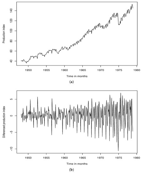
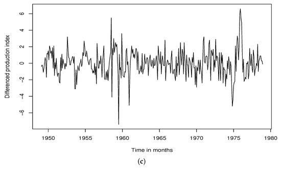
Figure 1. Plots of FRB production index time series. (a) FRB production index. (b) Nonseasonal differenced FRB production index. (c) Nonseasonal and seasonal differenced FRB production index.

We present the Bayesian subset selection results of the SAR models for the differenced FRB production index in Table 6, and we also display the estimation results in Table 7. As can be seen from Table 6, for the nonseasonal latent variables ${\mathit{\delta }}_{\mathbf{1}}$, the values $(1,0,0,0,0)$ had the highest frequency among all the possible values with a percentage of about 45.3%. For the seasonal latent variables ${\mathit{\delta }}_{\mathbf{2}}$, the values $(1,1,1,1,0)$ had the highest frequency with a percentage of about 37.5%, but another set of values $(1,1,1,0,0)$ had a very similar frequency with a percentage of about 36%. Thus, in this case, we had to look at the estimation results to check the significance of the SAR model coefficients using the 95% credible interval to decide between these two subsets of the SAR model. As we can see from Table 7, for the nonseasonal AR coefficients, only the first coefficient, i.e., ${\varphi }_{11}$, was significant, and all other nonseasonal AR coefficients were insignificant. On the other hand, for the seasonal AR coefficients, the first three coefficients, i.e., ${\varphi }_{21}$, ${\varphi }_{22}$, and ${\varphi }_{23}$, were significant, which supported the selection of $(1,1,1,0,0)$, not $(1,1,1,1,0)$. Therefore, for the differenced FRB production index, the SAR(1)(3)${}_{12}$ was selected as the best subset of the SAR model. For the sake of comparison, we also applied the AIC and AIC${}_c$ to select the best subset, and the results show that both methods selected the same subset, SAR(2)(4)${}_{12}$, which was very close to our algorithm selection.

Table 6. Bayesian subset selection results for the differenced FRB production index.

Nonseasonal Latent Variables			Seasonal Latent Variables
${\mathit{\delta }}_{\mathbf{1}}$	Freq	Percent	${\mathit{\delta }}_{\mathbf{2}}$	Freq	Percent
(1,0,0,0,0)	453	45.3	(1,1,1,1,0)	375	37.5
(1,0,0,1,0)	115	11.5	(1,1,1,0,0)	358	35.8
(1,1,0,0,0)	113	11.3	(1,1,0,0,0)	109	10.9
(1,0,0,0,1)	102	10.2	(1,1,1,0,1)	58	5.8
(1,0,1,0,0)	59	5.9	(1,1,1,1,1)	55	5.5
(1,0,0,1,1)	32	3.2	(1,1,0,1,0)	20	2.0
(1,1,0,0,1)	24	2.4	(1,1,0,0,1)	20	2.0
(1,1,1,0,0)	20	2.0	(1,1,0,1,1)	5	0.5

Table 7. Bayesian estimates results for the differenced FRB production index.

Parameter	$\mathit{\mu }$	$\mathit{\sigma }$	L	U
${\varphi }_{11}$	0.309	0.065	0.178	0.430
${\varphi }_{12}$	0.073	0.057	−0.027	0.188
${\varphi }_{13}$	−0.006	0.051	−0.116	0.090
${\varphi }_{14}$	0.062	0.055	−0.043	0.179
${\varphi }_{15}$	−0.064	0.052	−0.177	0.031
${\varphi }_{21}$	−0.692	0.070	−0.827	−0.549
${\varphi }_{22}$	−0.614	0.089	−0.786	−0.441
${\varphi }_{23}$	−0.274	0.105	−0.475	−0.072
${\varphi }_{24}$	−0.132	0.092	−0.334	0.018
${\varphi }_{25}$	0.026	0.057	−0.089	0.135
${\sigma }^2$	1.387	0.108	1.196	1.609

5. Conclusions

In this paper, we developed a Bayesian subset selection of the SAR models based on the SSVS procedure and Gibbs sampler. By introducing latent variables for the nonseasonal and seasonal SAR model lags, we adopted and modified the SSVS procedure to select the best subset SAR model. We employed mixture–normal, inverse gamma, and Bernoulli priors for the SAR model coefficients, variance, and latent variables, respectively. By deriving full conditional posteriors of the SAR model parameters in the closed form, we introduced the Gibbs sampler along with SSVS to present an efficient algorithm for the subset selection of the SAR models. We performed a simulation study and a real application to evaluate the accuracy of the proposed algorithm, and the results of the simulation study confirmed its accuracy, while the results of the real application showed its applicability to select the best subset of the SAR model for real time series with seasonality. As part of future work, we plan to extend this work to select the best subset of time series models with multiple seasonalities, as introduced in [11], and also to select the best subset of multivariate autoregressive models, i.e., vector autoregressive models.

References

- Amin, A.A. Gibbs Sampling for Bayesian Prediction of SARMA Processes. Pak. J. Stat. Oper. Res. 2019, 15, 397–418. [Google Scholar] [CrossRef]
- Box, G.E.; Jenkins, G.M.; Reinsel, G.C.; Ljung, G.M. Time Series Analysis: Forecasting and Control; John Wiley & Sons: Hoboken, NJ, USA, 2015. [Google Scholar]
- Amin, A.A. Sensitivity to prior specification in Bayesian identification of autoregressive time series models. Pak. J. Stat. Oper. Res. 2017, 13, 699–713. [Google Scholar] [CrossRef]
- Akaike, H. A new look at the statistical model identification. IEEE Trans. Autom. Control. 1974, 19, 716–723. [Google Scholar] [CrossRef]
- Hurvich, C.M.; Tsai, C.L. Regression and time series model selection in small samples. Biometrika 1989, 76, 297–307. [Google Scholar] [CrossRef]
- McClave, J.T. Estimating the order of autoregressive models: The max X2 method. J. Am. Stat. Assoc. 1978, 73, 122–128. [Google Scholar]
- Penm, J.H.; Terrell, R. On the recursive fitting of subset autoregressions. J. Time Ser. Anal. 1982, 3, 43–59. [Google Scholar] [CrossRef]
- Thanoon, B. Subset threshold autoregression with applications. J. Time Ser. Anal. 1990, 11, 75–87. [Google Scholar] [CrossRef]
- Sarkar, A.; Kanjilal, P. On a method of identification of best subset model from full ar-model. Commun. Stat.-Theory Methods 1995, 24, 1551–1567. [Google Scholar] [CrossRef]
- Amin, A.A. Bayesian analysis of double seasonal autoregressive models. Sankhya B 2020, 82, 328–352. [Google Scholar] [CrossRef]
- Amin, A.A. Gibbs sampling for Bayesian estimation of triple seasonal autoregressive models. Commun. Stat.-Theory Methods 2022. [Google Scholar] [CrossRef]
- George, E.I.; McCulloch, R.E. Variable selection via Gibbs sampling. J. Am. Stat. Assoc. 1993, 88, 881–889. [Google Scholar] [CrossRef]
- Chen, C.W. Subset selection of autoregressive time series models. J. Forecast. 1999, 18, 505–516. [Google Scholar] [CrossRef]
- So, M.K.; Chen, C.W.; Liu, F.C. Best subset selection of autoregressive models with exogenous variables and generalized autoregressive conditional heteroscedasticity errors. J. R. Stat. Soc. Ser. (Appl. Stat.) 2006, 55, 201–224. [Google Scholar] [CrossRef]
- Chen, C.W.; Liu, F.C.; Gerlach, R. Bayesian subset selection for threshold autoregressive moving-average models. Comput. Stat. 2011, 26, 1–30. [Google Scholar] [CrossRef]
- Ismail, M.A.; Amin, A.A. Gibbs Sampling For SARMA Models. Pak. J. Stat. 2014, 30, 153–168. [Google Scholar]
- Barnett, G.; Kohn, R.; Sheather, S. Bayesian estimation of an autoregressive model using Markov chain Monte Carlo. J. Econom. 1996, 74, 237–254. [Google Scholar] [CrossRef]
- Barnett, G.; Kohn, R.; Sheather, S. Robust Bayesian Estimation Of Autoregressive–Moving-Average Models. J. Time Ser. Anal. 1997, 18, 11–28. [Google Scholar] [CrossRef]
- Ismail, M.A. Bayesian Analysis of Seasonal Autoregressive Models. J. Appl. Stat. Sci. 2003, 12, 123–136. [Google Scholar]
- Ismail, M.A. Bayesian Analysis of the Seasonal Moving Average Model: A Gibbs Sampling Approach. Jpn. J. Appl. Stat. 2003, 32, 61–75. [Google Scholar] [CrossRef]
- Amin, A.A.; Ismail, M.A. Gibbs Sampling for Double Seasonal Autoregressive Models. Commun. Stat. Appl. Methods 2015, 22, 557–573. [Google Scholar] [CrossRef]
- Amin, A.A. Bayesian Inference for Double Seasonal Moving Average Models: A Gibbs Sampling Approach. Pak. J. Stat. Oper. Res. 2017, 13, 483–499. [Google Scholar] [CrossRef]
- Amin, A.A. Gibbs Sampling for Double Seasonal ARMA Models. In Proceedings of the 29th Annual International Conference on Statistics and Computer Modeling in Human and Social Sciences, Cairo, Egypt, 28–30 March 2017. [Google Scholar]
- Amin, A.A. Full Bayesian analysis of double seasonal autoregressive models with real applications. J. Appl. Stat. 2023, 1–21. [Google Scholar] [CrossRef]
- Amin, A.A. Bayesian Inference of Triple Seasonal Autoregressive Models. Pak. J. Stat. Oper. Res. 2022, 18, 853–865. [Google Scholar] [CrossRef]
- Raftery, A.E.; Lewis, S.M. The number of iterations, convergence diagnostics and generic Metropolis algorithms. Pract. Markov Chain. Monte Carlo 1995, 7, 763–773. [Google Scholar]
- Geweke, J. Evaluating the accuracy of sampling-based approaches to the calculations of posterior moments. Bayesian Stat. 1992, 4, 641–649. [Google Scholar]
- LeSage, J.P. Applied Econometrics Using MATLAB; Technical Report; Department of Economics, University of Toronto: Toronto, ON, Canada, 1999. [Google Scholar]
Disclaimer/Publisher’s Note: The statements, opinions and data contained in all publications are solely those of the individual author(s) and contributor(s) and not of MDPI and/or the editor(s). MDPI and/or the editor(s) disclaim responsibility for any injury to people or property resulting from any ideas, methods, instructions or products referred to in the content. |
© 2023 by the authors. Licensee MDPI, Basel, Switzerland. This article is an open access article distributed under the terms and conditions of the Creative Commons Attribution (CC BY) license (https://creativecommons.org/licenses/by/4.0/).