Heavy-Ball-Based Hard Thresholding Pursuit for Sparse Phase Retrieval Problems

Abstract

We introduce a novel iterative algorithm, termed the Heavy-Ball-Based Hard Thresholding Pursuit for sparse phase retrieval problem (SPR-HBHTP), to reconstruct a sparse signal from a small number of magnitude-only measurements. Our algorithm is obtained via a natural combination of the Hard Thresholding Pursuit for sparse phase retrieval (SPR-HTP) and the classical Heavy-Ball (HB) acceleration method. The robustness and convergence for the proposed algorithm were established with the help of the restricted isometry property. Furthermore, we prove that our algorithm can exactly recover a sparse signal with overwhelming probability in finite steps whenever the initialization is in the neighborhood of the underlying sparse signal, provided that the measurement is accurate. Extensive numerical tests show that SPR-HBHTP has a markedly improved recovery performance and runtime compared to existing alternatives, such as the Hard Thresholding Pursuit for sparse phase retrieval problem (SPR-HTP), the SPARse Truncated Amplitude Flow (SPARTA), and Compressive Phase Retrieval with Alternating Minimization (CoPRAM).

1. Introduction

In many engineering problems, one wishes to reconstruct signals from the (squared) modulus of its Fourier (or any linear) transform. This is called phase retrieval (PR). Particularly, if the target signal is sparse, this is referred to a sparse phase retrieval problem. The corresponding mathematical model is used to recover a sparse vector $x\in {\mathbb{R}}^n$ from a system of phaseless quadratic equations taking the form

$$y_i = |⟨a_i,x⟩{|,i=1,2,\dots ,m,\mathrm{subject}\mathrm{to}\parallel x\parallel }_0\le s,$$

(1)

where ${\left\{{\alpha }_i\right\}}_{i=1}^m$ are a set of n-dimensional sensing vectors, ${\left\{y_i\right\}}_{i=1}^m$ for $i=1,2,\dots ,m$ are observed modulus data, and s is the sparsity level (s is much less than n and is assumed to be known a priori for theoretical analysis purposes). As a matter of fact, solving the above problem is conducted to solve the following optimization system with the optimal value equal to zero

$$\begin{array}{c}\hfill min\frac{1}{2} \Vert y - \left|Ax\right| {\Vert }_2^{2}s.t.{\parallel x\parallel }_0\le s,\end{array}$$

(2)

where the measurement matrix A and observed data y are processed as follows:

$$\begin{array}{c}\hfill A:=\frac{1}{\sqrt{m}}{\left[\begin{array}{cccc}{a}_1& a_2& \dots & a_m\end{array}\right]}^T\in {\mathbb{R}}^{m\times n},y:=\frac{1}{\sqrt{m}}{\left[\begin{array}{cccc}{y}_1& y_2& \dots & y_m\end{array}\right]}^T.\end{array}$$

(3)

The phase retrieval problem arises naturally in many important applications, such as X-ray crystallography, microscopy, and astronomical imaging, etc. Interested readers are referred to [1] and its references for a more detailed discussion of the scientific and engineering background of the model.

Although several heuristic methods [2,3,4,5] are commonly used to solve (1), it is generally accepted that (1) is a very challenging, ill-posed, nonlinear inverse problem in both theory and practice. In particular, (1) is an NP-hard problem  [6]. At present, phase retrieval approaches can be mainly categorized as convex and nonconvex. A popular class of nonconvex approaches is based on alternating projections, e.g., the groundbreaking works by Gerchberg and Saxton [2], Fienup [3], Chen et al. [7], and Waldspurger [8]. The convex alternatives either rely on the so-called Shor’s relaxation to obtain a solver based on semidefinite programming (SDP), known simply as PhaseLift [9] and PhaseCut [10], or solve the problem of basis pursuit in dual domains, as conducted in PhaseMax [11,12]. Next, a series of breakthrough results [9,13,14,15] provided provably valid algorithmic processes for special cases, where the measurement vectors are randomly derived from some certain multivariate probability distribution, such as the Gaussian distributions. Phase retrieval problems [9,13,14] require the number of observations m to exceed the problem dimension n. However, for the sparse phase retrieval problem, the true signal can be successfully recovered, even if the number of measurements m is less than the length of the signal n. In particular, a recent paper [16] utilized the random sampling technique to achieve the best empirical sampling complexity; in other words, it requires less measurements than state-of-the-art algorithms for sparse phase retrieval problems. For more on phase recovery, interested readers can refer to [17,18,19,20,21,22,23,24,25,26,27].

There is a close relationship between the phase recovery problem and the compressed sensing problem [28,29,30]. Compressed sensing, also known as compressed sampling, is a new information technology used to find sparse solutions to underdetermined linear systems. Its corresponding mathematical model can be expressed as finding a sparse vector x from the following linear problem with sparsity constraints

$$y_i=⟨a_i,x⟩,i=1,2,\dots ,m,\mathrm{subject}\mathrm{to}{\parallel x\parallel }_0\le s.$$

(4)

Some mainstream algorithms for solving this problem have been proposed, including Iterative Hard Thresholding (IHT) [31], the Orthogonal Matching Pursuit (OMP) [32], the Compressive Sampling Matching Pursuit (CoSaMP) [33], the Subspace Pursuit (SP) [34], and the Hard Thresholding Pursuit (HTP)  [29]. The optimization model for the problem (4) is

$$\begin{array}{c}\hfill min\frac{1}{2}{\Vert y-Ax\Vert }_2^{2}s.t.{\parallel x\parallel }_0\le s.\end{array}$$

(5)

Comparing two problems, (1) and (4), we see that problem (1) has an extra absolute value over problem (4). This makes the objective function of system (2) nonsmooth compared to system (5). Accordingly, this leads to a huge difference in the design of our algorithms. How can we naturally modify the compressed sensing algorithm to solve the phase recovery problem? Recently, a breakthrough in this direction was the algorithm (we call it SPR-HTP) proposed in [15], which is a modification of HTP from linear measurements to phaseless measurements. Inspired by [15], we think that an acceleration method could be used to accelerate SPR-HTP. The Heavy-Ball was first introduced by Polyak [35], and it is an old as well as efficient way to speed things up. More recently, in [36], the authors combined the Heavy-Ball acceleration method with the classic HTP to obtain the HBHTP for solving compressed sensing. Their numerical experiment shows that the HBHTP performs better than the classical HTP in terms of the recovery capability and runtime.

Considering the above motivation, we propose, in this paper, a novel nonconvex algorithm to offset the disadvantages of existing algorithms. The new algorithm is called the Heavy-Ball-Based Hard Thresholding Pursuit for sparse phase retrieval problem (SPR-HBHTP). Similar to the most of the existing nonconvex algorithms, our proposed algorithm is divided into two stages: the initialization part and the iteration part. The optimization model (2) could have multiple local minimizers due to its nonconvexity. Hence, the initialization step is crucial to ensure the initial point can fall within a certain neighborhood of the real signal. Common initialization methods are orthogonality-promoting initialization, spectral initialization, variant of the spectral initialization, etc. In our algorithm, we adopt off-the-shelf spectral initialization as the initial step. For more details, please refer to reference [15]. For the iterative refinement stage, the search direction for SPR-HTP is

$$\alpha A^T\left(y\odot \mathrm{sgn}\left(A{x}^n\right)-A{x}^n\right),$$

where ⊙ represents the Hadamard product (the definition is given below) of two vectors, and $\alpha >0$ is a positive parameter. Our algorithm SPR-HBHTP is a combination of SPR-HTP and the Heavy-Ball method, and the search direction is represented as

$$\alpha A^T\left(y\odot \mathrm{sgn}\left(A{x}^n\right)-A{x}^n\right)+\beta (x^n-x^{n-1})$$

with two parameters $\alpha >0$, $\beta \ge 0$. Clearly SPR-HBHTP reduces to SPR-HTP as $\beta =0$. The following theoretical and numerical experiments show that the modified algorithm (SPR-HBHTP) using the momentum term $x^n-x^{n-1}$ matches the best available state-of-the-art sparse phase retrieval methods. With the help of the restricted isometry property (RIP) [37], the convergence of our algorithm is established, and our algorithm is proved to have robust sparse signal recovery under inaccurate measurement conditions. Moreover, our algorithm can exactly recover a s-sparse signal in finite steps if the measurement is accurate.

Our contributions in this paper are as follows: we propose a new class of HTP-type algorithms called the Heavy-Ball-Based Hard Thresholding Pursuit for sparse phase retrieval problem (SPR-HBHTP), which is a natural combination of the Hard Thresholding Pursuit for sparse phase retrieval (SPR-HTP) and the classical Heavy-Ball (HB) acceleration method. In the theoretical analysis, a new theoretical analysis framework is introduced to establish the theoretical performance results of the proposed algorithm by resorting to the restricted isometry property of measurement matrices. The local convergence of our algorithm is established regardless of whether there is noise in the measurement. An estimation of the iteration number is established under the framework of accurate measurements. For the aspect of numerical experiments, the phase transition curves, grayscale maps, and algorithm selection maps demonstrate that the new algorithm SPR-HBHTP is numerically much more efficient than existing alternatives, such as SPR-HTP, SPARTA, and CoPRAM in terms of both the recovery success rate and the recovery time.

The rest of the paper is organized as follows: we describe the SPR-HBHTP in Section 2. A theoretical analysis of the proposed algorithm is conducted in Section 3. Numerical experiments to illustrate the performance of the algorithm are given in Section 4, and conclusions are drawn in the last section.

2. Preliminary and Algorithms

2.1. Notations

We introduce some notations that are used throughout the paper. Let $\left[N\right]$ denote the set $\left\{1,2,\dots ,N\right\}$ and $\left|S\right|$ be the cardinality of a set S. Denote by $\overline{S}$ the complement $\left[N\right]\backslash S$ of a set S in $\left[N\right]$. At $x\in {\mathbb{R}}^n$, the signum function $\mathrm{sgn}\left(x\right)\in {\mathbb{R}}^n$ is defined as

$${\left[\mathrm{sgn}\left(x\right)\right]}_i:=\left\{\begin{array}{cc}1\hfill & x_i>0,\hfill \\ 0\hfill & x_i=0,\hfill \\ -1\hfill & x_i<0.\hfill \end{array}\right.$$

The Hard Thresholding operator $H_s\left(x\right)$ keeps the s largest absolute entries and sets other ones to zeros. For an index set $\Omega \subseteq \left[N\right]$, $A_{\Omega }$ denotes the matrix obtained from $A\in {\mathbb{R}}^{m\times n}$ by keeping only the columns indexed by $\Omega$, and $x_{\Omega }$ stands for the vector obtained by retaining the components of x indexed by $\Omega$ and zeroing out the remaining components of x. The set $\mathrm{supp}\left(x\right):=\left\{i\in \left[N\right]:x_i\ne 0\right\}$ is called the support of x, and $L_s\left(x\right)$ stands for the support of $H_s\left(x\right)$. For two sets, S and $\tilde{S}$, $S△\tilde{S}:=(S\backslash \tilde{S})\bigcup (\tilde{S}\backslash S)$ is the symmetric difference between S and $\tilde{S}$. For $x,z\in {\mathbb{R}}^n$, the distance between x and z is defined as

$$\mathrm{dist}(x,z):=\min \left\{{\parallel x-z\parallel }_2,{\parallel x+z\parallel }_2\right\}.$$

(6)

The notation ⊙ represents the Hadamard product of two vectors, i.e.,

$$a\odot b:={\left(a_1{b}_1,a_2{b}_2,\dots ,a_n{b}_n\right)}^T.$$

2.2. New Algorithms

The alternative initialization methods include orthogonality-promoting initialization [38], spectral initialization [39], or the other initialization [40], etc. In this paper, we use spectral initialization to constitute the initial step of the algorithm.

Algorithm 1: Heavy-Ball-Based Hard Thresholding Pursuit for sparse phase retrieval (SPR-HBHTP).

Input: a matrix ${\left\{a_i\right\}}_{i=1}^m$, a vector ${\left\{y_i\right\}}_{i=1}^m$, and two parameters $\alpha >0$ and $\beta \ge 0$. Initialization: $${\varphi }^2:=\frac{1}{m}\sum _{i=1}^m{y}_i^2,v_j:=\frac{1}{m}\sum _{i=1}^m{y}_i^2{a}_{ij}^2,j=1,\dots n,\tilde{S}:=L_S\left(v\right),$$ $$W:=\frac{1}{m}\sum _{i=i}^m{y}_i^2{\left[a_i\right]}_{\tilde{S}}{\left[a_i\right]}_{\tilde{S}}^T,x^0:=\varphi \tilde{u},$$ where $\tilde{u}$ is the unit principal eigenvector of W. Set $x^1=x^0$. Repeat: $$z^{n+1}=A{x}^n,y^{n+1}=y\odot \mathrm{sgn}\left(z^{n+1}\right),$$ $$S^{n+1}=\mathrm{supp}\left(H_s\left(x^n+\alpha A^T(y^{n+1}-z^{n+1})+\beta (x^n-x^{n-1})\right)\right),$$ $$x^{n+1}=arg\min \left\{\frac{1}{2}{\parallel Az-y^{n+1}\parallel }_2^2:\mathrm{supp}\left(z\right)\subseteq S^{n+1}\right\}.$$ Output: the s-sparse vector $x.$

The following is a brief explanation of initialization in the Algorithm 1. For a more rigorous and in-depth discussion of this aspect, please refer to [15,39].

Estimate the support: Since $E\left[\frac{1}{m}{\sum }_{i=1}^m{y}_i^2{a}_{ij}^2\right]$ = ${\parallel x\parallel }_2^2+2x_j^2$, $\tilde{S}=L_s\left({\left\{\frac{1}{m}{\sum }_{i=1}^m{y}_i^2{a}_{ij}^2\right\}}_{j=1}^n\right)$ contains a mass of correct support, it could be a good approximation of the support of x.

Compute the signal: Note that

$$E\left[\frac{1}{m}\sum _{i=i}^m{y}_i^2{a}_i{a}_i^T\right]=\left(I+2\frac{x}{{\parallel x\parallel }_2}·\frac{x^T}{{\parallel x\parallel }_2}\right){\parallel x\parallel }_2^2,E\left[\frac{1}{m}\sum _{i=1}^m{y}_i^2\right]=E\left[{\parallel y\parallel }_2\right]={\parallel x\parallel }_2.$$

Hence, the principal eigenvector of the matrix W in Algorithm 1 gives a good initial direction guess of the true signal x. We select the principal eigenvector vector with a length of ${\parallel y\parallel }_2$ as the initial point $x^0$ to ensure that the power of the initial estimate $x^0$ is close to that of the true signal x.

The most important conclusion of the initialization process is that the initial point can fall within a certain neighborhood of the real signal relative to the distance measurement defined in (6).

Lemma 1 

([39] [Theorem IV.1]). Let ${\left\{a_i\right\}}_{i=1}^m$ be i.i.d Gaussian random vectors with a mean of 0 and variance matrix of I. Let $x_0$ be generated by initialization in Algorithm 1 with the input $y_i=\left|a_i^{T}x\right|$ for $i=1,\dots ,m$, where $x\in R^n$ is a signal satisfying ${\parallel x\parallel }_0\le s$. Then, for any ${\lambda }_0\in (0,1)$, there exists a positive constant C depending only on ${\lambda }_0\in (0,1)$, such that if $m\ge C{s}^{2}logn$, we have

$$\mathrm{dist}(x_0,x)\le {\lambda }_0{\parallel x\parallel }_2$$

with a probability of at least $1-8m^{-1}$.

3. Convergence Analysis

We first list some of the main Lemmas and present our results on the local convergence of the proposed algorithm (SPR-HBHTP).

Lemma 2 

([30] [Theorem 9.27]). Let ${\left\{a_i\right\}}_{i=1}^m$ be i.i.d Gaussian random vectors with a mean of 0 and variance matrix of I. Let A be defined in (3). Some universal positive constants $C_1$, $C_2$ exist, such that for any natural number $r\le n$ and any ${\delta }_r\in (0,1)$, if $m\ge C_1{\delta }_r^{-2}rlog(n/r)$, then A satisfies the following r-RIP with a probability of at least $1-e^{-C_{2}m}$,

$$\begin{array}{c}\hfill \left(1-{\delta }_r\right){\parallel x\parallel }_2^2\le {\parallel Ax\parallel }_2^2\le \left(1+{\delta }_r\right){\parallel x\parallel }_2^2,\forall {\parallel x\parallel }_0\le r.\end{array}$$

(7)

Lemma 3 

([36] [Lemma 3.1]). Suppose that the non-negative sequence $\left\{{\tau }^n\right\}\subseteq \mathbb{R}$$(n=0,1,...)$ satisfies

$$\begin{array}{c}\hfill {\tau }^{n+1}\le b_1{\tau }^n+b_2{\tau }^{n-1}+b_3,n\ge 1,\end{array}$$

(8)

where $b_1,b_2,b_3\ge 0$ and $b_1+b_2<1$. Then,

$$\begin{array}{c}\hfill {\tau }^n\le {\theta }^{n-1}\left[{\tau }^1+\left(\theta -b_1\right){\tau }^0\right]+\frac{b_3}{1-\theta }\end{array}$$

with

$$0\le \theta :=\frac{b_1+\sqrt{b_1^2+4b_2}}{2}<1.$$

Lemma 4 

([29,41]). Let $u\in {\mathbb{R}}^n$, $v\in {\mathbb{R}}^m$ and $S\subseteq \{1,\dots ,n\}$. Assume that the condition (7) holds.

(i).

If $|S\cup supp(u\left)\right|\le r$, then

$$\begin{array}{c}\hfill {\parallel {\left((I-A^{T}A)u\right)}_S\parallel }_2\le {\delta }_r{\parallel u\parallel }_2.\end{array}$$

(9)

(ii).

If $\left|S\right|\le r$, then

$${\parallel {\left(A^{T}v\right)}_S\parallel }_2\le \sqrt{1+{\delta }_r}{\parallel v\parallel }_2.$$

(10)

Lemma 5 

([15] [Lemma 2]). Let ${\left\{a_i\right\}}_{i=1}^m$ be i.i.d. Gaussian random vectors with a mean of 0 and variance matrix of I. Let ${\lambda }_0$ be any constant in $(0,\frac{1}{8}]$. After fixing any given ${\epsilon }_0>0$, the universal positive constants $C_3$, $C_4$ exist. If

$$m\ge C_{3}slog\left(n/s\right),$$

then with a probability of at least $1-e^{-C_{4}m}$, it holds that

$$\begin{array}{c}\hfill \frac{1}{m}\sum _{i=1}^m|a_i^T{x}^{♮}{|}^2·1_{\left\{\left(a_i^{T}x\right)\left(a_i^T{x}^{♮}\right)\le 0\right\}}\le \frac{1}{{\left(1-{\lambda }_0\right)}^2}{\left({\epsilon }_0+{\lambda }_0\sqrt{\frac{21}{20}}\right)}^2{\parallel x-x^{♮}\parallel }_2^2,\end{array}$$

(11)

whenever $x,x^{♮}$ satisfies ${\parallel x\parallel }_0\le s$ and $\parallel x-x^{♮}{\parallel }_2\le {\lambda }_0{\parallel x^{♮}\parallel }_2$.

Lemma 6. 

Let ${\left\{a_i\right\}}_{i=1}^m$ be i.i.d. Gaussian random vectors with a mean of 0 and variance matrix of I. Let $z,x,\widehat{y},{\lambda }_0$ be given as

$$\widehat{y}={\left|Ax\right|\odot \mathrm{sgn}\left(Az\right),\parallel z-x\parallel }_2\le {\lambda }_0{\parallel x\parallel }_2,{\parallel z\parallel }_0\le s,{\lambda }_0\in (0,\frac{1}{8}].$$

For any ${\epsilon }_0>0$, the universal positive constants $C_5$ and $C_6$ exist, such that if

$$\begin{array}{c}\hfill m\ge C_{5}slog(n/s),\end{array}$$

(12)

then the following inequality holds with a probability of at least $1-e^{-C_{6}m}:$

$$\parallel {\left(A^T(\widehat{y}-Ax)\right)}_S{\parallel }_2\le \theta \left({\lambda }_0\right)\sqrt{1+{\delta }_s}{\parallel z-x\parallel }_2,$$

where $\theta \left({\lambda }_0\right):=\frac{2}{1-{\lambda }_0}\left({\epsilon }_0+{\lambda }_0\sqrt{\frac{21}{20}}\right)$ and $S\subset \left\{1,2,\dots ,m\right\}$ with $\left|S\right|\le s$.

Proof of Lemma 6.

Pick $C_5:=max\{C_1{\delta }_s^{-2},C_3\}$, where $C_1,C_3$ comes from Lemmas 2 and 5. The condition (12) ensures the validity of (7) with a probability of at least $1-e^{-C_{2}m}$ and (11) with a probability of at least $1-e^{-C_{4}m}$, respectively. Let

$$C_6:=\frac{ln\left(e^{-C_{2}m}+e^{-C_{4}m}-e^{-\left(C_2+C_4\right)m}\right)}{-m}.$$

It is easy to see that $\left(1-e^{-C_{2}m}\right)\left(1-e^{-C_{4}m}\right)=1-e^{-C_{6}m}$. In other words, the probability of (7) and (11) being true is at least $1-e^{-C_{6}m}$. By replacing $y_{k+1}$, $x_k$ and $x^{♮}$ used in [15] [Equation (16)] by $\widehat{y}$, z and x, we obtain

$$\parallel \widehat{y}{-Ax\parallel }_2^2\le \frac{4}{{\left(1-{\lambda }_0\right)}^2}{\left({\epsilon }_0+{\lambda }_0\sqrt{\frac{21}{20}}\right)}^2{\parallel z-x\parallel }_2^2=\theta {\left({\lambda }_0\right)}^2{\parallel z-x\parallel }_2^2.$$

This, together with (10) in Lemma 4, leads to

$$\parallel {\left(A^T\left(\widehat{y}-Ax\right)\right)}_S{\parallel }_2\le \sqrt{1+{\delta }_s}\parallel \widehat{y}{-Ax\parallel }_2\le \theta \left({\lambda }_0\right)\sqrt{1+{\delta }_s}{\parallel z-x\parallel }_2.$$

□

The local convergence property of Algorithm 1 is established in the following result.

Theorem 1. 

(Local convergence). Let ${\left\{a_i\right\}}_{i=1}^m$ be i.i.d. Gaussian random vectors with a mean of 0 and variance matrix of I. Let ${\lambda }_0$ be any constant in $(0,\frac{1}{8}]$. Suppose that the RIC, ${\delta }_{3s}$, of matrix A and the parameters α and β obey

$$\begin{array}{c}\hfill 0<{\delta }_{3s}<{\delta }^{♯},0\le \beta <\frac{\frac{1}{\eta }+1-\frac{\theta \left({\lambda }_0\right)\sqrt{1+{\delta }_s}}{\eta \left(1-{\delta }_{2s}\right)}}{1+{\delta }_{3s}+\theta \left({\lambda }_0\right)\sqrt{1+{\delta }_{2s}}}-1,\end{array}$$

(13)

$$\begin{array}{c}\hfill \frac{1+2\beta -\frac{1}{\eta }+\frac{\theta \left({\lambda }_0\right)\sqrt{1+{\delta }_s}}{\eta \left(1-{\delta }_{2s}\right)}}{1-{\delta }_{3s}-\theta \left({\lambda }_0\right)\sqrt{1+{\delta }_{2s}}}<\alpha <\frac{\frac{1}{\eta }+1-\frac{\theta \left({\lambda }_0\right)\sqrt{1+{\delta }_s}}{\eta \left(1-{\delta }_{2s}\right)}}{1+{\delta }_{3s}+\theta \left({\lambda }_0\right)\sqrt{1+{\delta }_{2s}}},\end{array}$$

(14)

where

$$\begin{array}{c}\hfill \theta \left({\lambda }_0\right):=\frac{2}{1-{\lambda }_0}\left({\epsilon }_0+{\lambda }_0\sqrt{\frac{21}{20}}\right),{\epsilon }_0:={10}^{-3},\eta :=\frac{\sqrt{2}}{\sqrt{1-{\delta }_{2s}^2}},\end{array}$$

(15)

and ${\delta }^{♯}$ is the unique root in the interval $(0,1)$ of the equation $\gamma \left(x\right)=\theta \left({\lambda }_0\right)$ with

$$\gamma \left(x\right):=\frac{\left(1-x\right)\sqrt{1+x}-x\sqrt{2\left(1-x\right)}}{1+x+\sqrt{2\left(1-x^2\right)}}.$$

For a s-sparse signal $x\in {\mathbb{R}}^n$, the universal positive constants $C_7$, $C_8$ exist, such that if

$$m\ge C_{7}slog(n/s),\mathrm{dist}(x^0,x)\le {\lambda }_0{\parallel x\parallel }_2,$$

then the sequence $\left\{x^n\right\}$ generated by Algorithm 1 with input measured data $y=\left|Ax\right|$ satisfies

$$\begin{array}{c}\hfill \mathrm{dist}(x^{n+1},x)\le {\tau }^n\left(min\{\parallel x^1-x{\parallel }_2+(\tau -b)\parallel x^0-x{\parallel }_2,\parallel x^1+x{\parallel }_2+(\tau -b)\parallel x^0+x{\parallel }_2\}\right)\end{array}$$

(16)

with a probability of at least ${(1-e^{-C_{8}m})}^n$, where

$$\begin{array}{c}\hfill \tau :=\frac{b+\sqrt{b^2+4\eta \beta }}{2},b:=\eta \left(\left|1-\alpha +\beta \right|+\alpha \left({\delta }_{3s}+\theta \left({\lambda }_0\right)\sqrt{1+{\delta }_{2s}}\right)\right)+\frac{\theta \left({\lambda }_0\right)\sqrt{1+{\delta }_s}}{1-{\delta }_{2s}},\end{array}$$

(17)

and $\tau <1$ is guaranteed under the conditions (13) and (14).

Proof of Theorem 1. 

Note that $x_0=x_1$ in the design of Algorithm 1 and $x_0$ is generated by utilizing the initialization process. Hence, $\mathrm{dist}(x^0,x)=\mathrm{dist}(x^1,x)\le {\lambda }_0{\parallel x\parallel }_2$ by Lemma 1. Since $\mathrm{dist}(x^0,x)=min\{\parallel x^0{-x\parallel }_2,\parallel x^0+x\parallel \}$, we can assume without a loss of generalization that $\mathrm{dist}(x^0,x)={\parallel x^0-x\parallel }_2$ (the case of $\mathrm{dist}(x^0,x)={\parallel x^0+x\parallel }_2$ can be proved by following a similar argument). Hence, $\parallel x^0{-x\parallel }_2\le {\lambda }_0{\parallel x\parallel }_2$, $\parallel x^1{-x\parallel }_2\le {\lambda }_0{\parallel x\parallel }_2$. Our proof is based on mathematical induction, and hence, we further assume that $\parallel x^{n-1}{-x\parallel }_2\le {\lambda }_0{\parallel x\parallel }_2$, $\parallel x^n{-x\parallel }_2\le {\lambda }_0{\parallel x\parallel }_2$.

The first step of the proof is a consequence of the pursuit step of Algorithm 1. Recall that

$$\begin{array}{c}\hfill x^{n+1}=\mathrm{argmin}\left\{\frac{1}{2}{\parallel y^{n+1}-Az\parallel }_2^2:\mathrm{supp}\left(z\right)\subset S^{n+1}\right\}.\end{array}$$

As the best $l_2$-approximation to $y^{n+1}$ from the space $\left\{Az|\mathrm{supp}\left(z\right)\subset S^{n+1}\right\}$, the vector $x^{n+1}$ is characterized by

$$⟨y^{n+1}-A{x}^{n+1},Az⟩=0\mathrm{whenever}\mathrm{supp}\left(z\right)\subset S^{n+1},$$

i.e., $⟨A^T(y^{n+1}-A{x}^{n+1}),z⟩=0$ $\mathrm{whenever}\mathrm{supp}\left(z\right)\subset S^{n+1}$ or ${\left(A^T(y^{n+1}-A{x}^{n+1})\right)}_{S^{n+1}}=0$. We derive, in particular,

$$\begin{array}{cc}\hfill & \parallel {(x^{n+1}-x)}_{S^{n+1}}{\parallel }_2^2\hfill \\ \hfill & =⟨{(x^{n+1}-x)}_{S^{n+1}},{(x^{n+1}-x)}_{S^{n+1}}⟩\hfill \\ \hfill & =⟨{(x^{n+1}-x)}_{S^{n+1}},{\left(x^{n+1}-x+A^T(y^{n+1}-A{x}^{n+1})\right)}_{S^{n+1}}⟩\hfill \\ \hfill & =⟨{(x^{n+1}-x)}_{S^{n+1}},{\left[(I-A^{T}A)(x^{n+1}-x)\right]}_{S^{n+1}}⟩+⟨{(x^{n+1}-x)}_{S^{n+1}},{\left(A^T(y^{n+1}-Ax)\right)}_{S^{n+1}}⟩\hfill \\ \hfill & \le \parallel {(x^{n+1}-x)}_{S^{n+1}}{\parallel }_2\left\{\parallel {\left[(I-A^{T}A)(x^{n+1}-x)\right]}_{S^{n+1}}{\parallel }_2+{\parallel {\left(A^T(y^{n+1}-Ax)\right)}_{S^{n+1}}\parallel }_2\right\}.\hfill \end{array}$$

(18)

Due to $\mathrm{supp}\left(x^{n+1}\right)\subseteq S^{n+1}$, $\left|\mathrm{supp}\left(x^{n+1}-x\right)\cup S^{n+1}\right|\le 2s$ and $|S^{n+1}|\le s$. It follows from Lemmas 4 and 6 that if $m\ge max\{C_1{\delta }_{2s}^{-2}\left(2s\right)\log (n/2s),C_{5}s\log (n/s)\}$, then

$$\begin{array}{c}\hfill \parallel {\left((I-A^{T}A)(x^{n+1}-x)\right)}_{S^{n+1}}{\parallel }_2\le {\delta }_{2s}{\parallel x^{n+1}-x\parallel }_2\end{array}$$

(19)

with a probability of at least $1-e^{-C_{2}m}$ and

$$\begin{array}{c}\hfill \parallel {\left(A^T(y^{n+1}-Ax)\right)}_{S^{n+1}}{\parallel }_2\le \theta \left({\lambda }_0\right)\sqrt{1+{\delta }_s}{\parallel x^n-x\parallel }_2\end{array}$$

(20)

with a probability of at least $1-e^{-C_{6}m}$. Combining (18), (19) with (20) leads to

$$\parallel {(x^{n+1}-x)}_{S^{n+1}}{\parallel }_2\le {\delta }_{2s}\parallel x^{n+1}{-x\parallel }_2+\theta \left({\lambda }_0\right)\sqrt{1+{\delta }_s}{\parallel x^n-x\parallel }_2.$$

(21)

Hence,

$$\begin{array}{cc}\hfill \parallel x^{n+1}{-x\parallel }_2^2& =\parallel {(x^{n+1}-x)}_{\overline{S^{n+1}}}{\parallel }_2^2+{\parallel {(x^{n+1}-x)}_{S^{n+1}}\parallel }_2^2\hfill \\ \hfill & \le \parallel {(x^{n+1}-x)}_{\overline{S^{n+1}}}{\parallel }_2^2+{\left({\delta }_{2s}\parallel x^{n+1}{-x\parallel }_2+\theta \left({\lambda }_0\right)\sqrt{1+{\delta }_s}{\parallel x^n-x\parallel }_2\right)}^2.\hfill \end{array}$$

Denote $\vartheta :=\theta \left({\lambda }_0\right)\sqrt{1+{\delta }_s}{\parallel x^n-x\parallel }_2$. This reads as $g(\parallel x^{n+1}-x{\parallel }_2)\le 0$ for the quadratic polynomial defined by

$$g\left(t\right):=(1-{\delta }_{2s}^2)t^2-2\vartheta {\delta }_{2s}t-(\parallel {(x^{n+1}-x)}_{\overline{S^{n+1}}}{\parallel }_2^2+{\vartheta }^2).$$

Hence, $\parallel x^{n+1}{-x\parallel }_2$ is bounded by the largest root of g, i.e.,

$$\parallel x^{n+1}{-x\parallel }_2\le \frac{\vartheta {\delta }_{2s}+\sqrt{(1-{\delta }_{2s}^2){\parallel {(x^{n+1}-x)}_{\overline{S^{n+1}}}\parallel }_2^2+{\vartheta }^2}}{1-{\delta }_{2s}^2}.$$

Based on $\sqrt{a^2+b^2}\le a+b$ for $a,b\ge 0$, we obtain

$$\begin{array}{c}\hfill \parallel x^{n+1}{-x\parallel }_2\le \frac{1}{\sqrt{1-{\delta }_{2s}^2}}{\parallel {(x^{n+1}-x)}_{\overline{S^{n+1}}}\parallel }_2+\frac{\vartheta }{1-{\delta }_{2s}}.\end{array}$$

(22)

The second step of the proof is a consequence of the Hard Thresholding step of Algorithm 1. Denote

$$\begin{array}{c}\hfill u^n:=x^n+\alpha A^T\left(y^{n+1}-A{x}^n\right)+\beta \left(x^n-x^{n-1}\right).\end{array}$$

(23)

Since $S^{n+1}=\mathrm{supp}\left(H_s\left(u^n\right)\right)$ and $S:=\mathrm{supp}\left(x\right)$, we have

$$\parallel {\left(u^n\right)}_{S^{n+1}}{\parallel }_2^2\ge {\parallel {\left(u^n\right)}_S\parallel }_2^2.$$

According to $S^{n+1}\backslash \left(S\cap S^{n+1}\right)=S^{n+1}\backslash S$ and $S\backslash \left(S\cap S^{n+1}\right)=S\backslash S^{n+1}$, we yield

$$\parallel {\left(u^n\right)}_{S^{n+1}\backslash S}{\parallel }_2^2\ge {\parallel {\left(u^n\right)}_{S\backslash S^{n+1}}\parallel }_2^2.$$

Taking ${\left(x\right)}_{S^{n+1}\backslash S}=0$ and ${\left(x^{n+1}\right)}_{S\backslash S^{n+1}}=0$ into consideration, we write

$$\parallel {(u^n-x)}_{S^{n+1}\backslash S}{\parallel }_2\ge \parallel {(x-x^{n+1}+u^n-x)}_{S\backslash S^{n+1}}{\parallel }_2\ge \parallel {(x-x^{n+1})}_{\overline{S^{n+1}}}{\parallel }_2-{\parallel {(u^n-x)}_{S\backslash S^{n+1}}\parallel }_2.$$

Hence,

$$\begin{array}{cc}\hfill \parallel {(x-x^{n+1})}_{\overline{S^{n+1}}}{\parallel }_2& \le \parallel {(u^n-x)}_{S\backslash S^{n+1}}{\parallel }_2+{\parallel {(u^n-x)}_{S^{n+1}\backslash S}\parallel }_2\hfill \\ \hfill & \le \sqrt{2\left(\parallel {(u^n-x)}_{S\backslash S^{n+1}}{\parallel }_2^2+{\parallel {(u^n-x)}_{S^{n+1}\backslash S}\parallel }_2^2\right)}\hfill \\ \hfill & =\sqrt{2}{\parallel {(u^n-x)}_{S^{n+1}△S}\parallel }_2.\hfill \end{array}$$

(24)

Note from (23) that

$$\begin{array}{cc}\hfill & u^n-x\hfill \\ \hfill & =x^n+\alpha A^T\left(y^{n+1}-A{x}^n\right)+\beta \left(x^n-x^{n-1}\right)-x\hfill \\ \hfill & =\left(1-\alpha +\beta \right)\left(x^n-x\right)-\beta \left(x^{n-1}-x\right)+\alpha \left(I-A^{T}A\right)\left(x^n-x\right)+\alpha A^T\left(y^{n+1}-Ax\right).\hfill \end{array}$$

Then,

$$\begin{array}{cc}\hfill & \parallel {\left(u^n-x\right)}_{S^{n+1}△S}{\parallel }_2\hfill \\ \hfill & \le \left|1-\alpha +\beta \right|·\parallel {(x^n-x)}_{S^{n+1}△S}{\parallel }_2+\alpha {\parallel {\left[(I-A^{T}A)(x^n-x)\right]}_{S^{n+1}△S}\parallel }_2\hfill \\ \hfill & +\alpha \parallel {\left(A^T(y^{n+1}-Ax)\right)}_{S^{n+1}△S}{\parallel }_2+\beta {\parallel {\left(x^{n-1}-x\right)}_{S^{n+1}△S}\parallel }_2\hfill \\ \hfill & \le \left(\left|1-\alpha +\beta \right|+\alpha {\delta }_{3s}+\alpha \theta \left({\lambda }_0\right)\sqrt{1+{\delta }_{2s}}\right)\parallel x^n{-x\parallel }_2+\beta {\parallel x^{n-1}-x\parallel }_2,\hfill \end{array}$$

(25)

where the second inequality is based on the fact that

$$\parallel {\left((I-A^{T}A)(x^n-x)\right)}_{S^{n+1}△S}{\parallel }_2\le {\delta }_{3s}{\parallel x^n-x\parallel }_2$$

(26)

with a probability of at least $1-e^{C_{2}m}$ as $m\ge C_1{\delta }_{3s}^{-1}\left(3s\right)\log (n/3s)$ by (9) in Lemma 4 due to $|S^{n+1}\Delta S\cup \mathrm{supp}\left(x^n-x\right)|\le 3s$, and

$$\parallel {\left(A^T(y^{n+1}-Ax)\right)}_{S^{n+1}△S}{\parallel }_2\le \theta \left({\lambda }_0\right)\sqrt{1+{\delta }_{2s}}{\parallel x^n-x\parallel }_2$$

(27)

with a probability of at least $1-e^{C_{6}m}$ as $m\ge C_5\left(2s\right)\log (n/2s)$ by Lemma 6 due to $|S^{n+1}△S|\le 2s$. Combining (24) with (25), we have

$$\begin{array}{cc}\hfill \parallel {(x-x^{n+1})}_{\overline{S^{n+1}}}{\parallel }_2& \le \sqrt{2}\left[\left(\left|1-\alpha +\beta \right|+\alpha {\delta }_{3s}+\alpha \theta \left({\lambda }_0\right)\sqrt{1+{\delta }_{2s}}\right){\parallel x^n-x\parallel }_2\right.\hfill \\ \hfill & +\left.\beta \parallel x^{n-1}{-x\parallel }_2\right].\hfill \end{array}$$

(28)

Putting (22) and (28) together yields

$$\begin{array}{cc}\hfill & \parallel x^{n+1}{-x\parallel }_2\hfill \\ \hfill & \le \left(\frac{\sqrt{2}\left(\left|1-\alpha +\beta \right|+\alpha {\delta }_{3s}+\alpha \theta \left({\lambda }_0\right)\sqrt{1+{\delta }_{2s}}\right)}{\sqrt{1-{\delta }_{2s}^2}}+\frac{\theta \left({\lambda }_0\right)\sqrt{1+{\delta }_s}}{1-{\delta }_{2s}}\right){\parallel x^n-x\parallel }_2\hfill \\ \hfill & +\frac{\sqrt{2}\beta }{\sqrt{1-{\delta }_{2s}^2}}{\parallel x^{n-1}-x\parallel }_2\hfill \\ \hfill & =b\parallel x^n{-x\parallel }_2+\eta \beta {\parallel x^{n-1}-x\parallel }_2,\hfill \end{array}$$

(29)

where b is given by (17). The recursive inequality (29) is in the form (8) in Lemma 3 by letting $b_3=0$. Note that, to ensure the validity of (19), (20), (26) and (27) with a corresponding probability of at least ${(1-e^{-C_{2}m})}^2{(1-e^{-C_{6}m})}^2$, the number of measurements must satisfy

$$m\ge max\{C_1{\delta }_{2s}^{-2}\left(2s\right)\log (n/2s),C_1{\delta }_{3s}^{-1}\left(3s\right)\log (n/3s),C_{5}s\log (n/s),C_5\left(2s\right)\log (n/2s)\}.$$

Hence, we can pick $C_7$ and $C_8$, satisfying

$$C_7\ge \max \left\{C_5,2C_5\left(1-\frac{log2}{log\left(n/s\right)}\right),2C_1{\delta }_{2s}^{-2}\left(1-\frac{log\left(2\right)}{log\left(n/s\right)}\right),3C_1{\delta }_{3s}^{-2}\left(1-\frac{log\left(3\right)}{log\left(n/s\right)}\right)\right\}$$

and

$$C_8\le \frac{1}{m}ln\left[\frac{1}{1-{(1-e^{-C_{2}m})}^2{(1-e^{-c_{6}m})}^2}\right].$$

In other words, the above choices of $C_7$ and $C_8$ guarantee that (19), (20), (26), and (27) hold with a probability of at least $(1-e^{-C_{8}m})$ as $m\ge C_{7}s\log (n/s)$. This, in turn, means that the (29) holds accordingly.

In the following, we need to show that the coefficients of the right-hand side of the (29) satisfy the conditions required for Lemma 3, i.e., $b+\eta \beta <1$.

First, we clarify that the parameters $\alpha ,\beta$ appearing in (13) and (14) are well-defined. On the interval $(0,1)$, define

$$\gamma \left(x\right):=\frac{\left(1-x\right)\sqrt{1+x}-x\sqrt{2\left(1-x\right)}}{1+x+\sqrt{2\left(1-x^2\right)}}\mathrm{and}g\left(x\right):=1+x+\sqrt{2\left(1-x^2\right)}.$$

Note that $g^{\prime }\left(x\right)=1-(2x/\sqrt{2(1-x^2)})$ and the root of $g^{\prime }\left(x\right)=0$ is $x=\sqrt{3}/3$. It is easy to see

$$max\{g\left(x\right):x\in (0,1)\}=g(\sqrt{3}/3)=1+\sqrt{3}.$$

Thus,

$$\gamma \left(x\right)=\frac{\left(1-x\right)\sqrt{1+x}-x\sqrt{2\left(1-x\right)}}{1+x+\sqrt{2\left(1-x^2\right)}}\ge \frac{\left(1-x\right)\sqrt{1+x}-x\sqrt{2\left(1-x\right)}}{1+\sqrt{3}}=:h\left(x\right).$$

(30)

Note that

$$h^{\prime }\left(x\right)=\frac{1}{1+\sqrt{3}}\left(\frac{-1-3x}{2\sqrt{1+x}}-\frac{2-3x}{\sqrt{2(1-x)}}\right).$$

(31)

Then, $h^{\prime }\left(x\right)=0$ is equivalent to saying that $(-1-3x)\sqrt{2(1-x)}=2(2-3x)\sqrt{(1+x)}$. Taking the square on both sides yields $(x-1/3)(27x^2-21)=27x^3-9x^2-21x+7=0$. The roots of the above equation in the interval $(0,1)$ are $x=1/3,\sqrt{7}/3$. By substituting these into (31), we obtain the root of $h^{\prime }\left(x\right)=0$ in (0,1) is $\sqrt{7}/3$. It is easy to see that h is monotonically decreasing on $(0,\sqrt{7}/3)$ and increasing on ($\sqrt{7}/3$,1). Due to $h\left(1\right)=0$, $h\left(x\right)<0$ as $x\in [\sqrt{7}/3,1)$ by the monotonicity of h. On the other hand, $\theta$ is monotonically increasing and $0\le \theta \left({\lambda }_0\right)\le \theta (1/8)\approx 0.295<0.366\approx h\left(0\right)$ as ${\lambda }_0\in (0,1/8]$. Hence for the given ${\lambda }_0\in (0,1/8]$ and $\theta \left({\lambda }_0\right)$, there is a unique solution in the interval $(0,\sqrt{7}/3)$, denoted by ${\delta }^{♯}$, satisfying $h\left(x\right)=\theta \left({\lambda }_0\right)$. In addition according to the decreasing monotonicity of h on this interval, we know $h\left(x\right)>\theta \left({\lambda }_0\right)$ for all $x\in (0,{\delta }^{♯})$. Thus, $h\left({\delta }_{3s}\right)>\theta \left({\lambda }_0\right)$ as ${\delta }_{3s}<{\delta }^{♯}$. This, together with (30), yields $\gamma \left({\delta }_{3s}\right)>\theta \left({\lambda }_0\right)$, i.e.,

$$\frac{\sqrt{1-{\delta }_{3s}^2}-\sqrt{2}{\delta }_{3s}}{\frac{1+{\delta }_{3s}}{\sqrt{1-{\delta }_{3s}}}+\sqrt{2\left(1+{\delta }_{3s}\right)}}=\frac{\left(1-{\delta }_{3s}\right)\sqrt{1+{\delta }_{3s}}-{\delta }_{3s}\sqrt{2\left(1-{\delta }_{3s}\right)}}{1+{\delta }_{3s}+\sqrt{2\left(1-{\delta }_{3s}^2\right)}}>\theta \left({\lambda }_0\right).$$

(32)

It follows from (32) that

$$\begin{array}{cc}\hfill \frac{\sqrt{1-{\delta }_{3s}^2}}{\sqrt{2}}-{\delta }_{3s}& >\theta \left({\lambda }_0\right)\frac{1+{\delta }_{3s}}{\sqrt{2(1-{\delta }_{3s})}}+\theta \left({\lambda }_0\right)\sqrt{1+{\delta }_{3s}}\hfill \\ \hfill & =\theta \left({\lambda }_0\right)\frac{\sqrt{1-{\delta }_{3s}^2}}{\sqrt{2}}\frac{\sqrt{1+{\delta }_{3s}}}{1-{\delta }_{3s}}+\theta \left({\lambda }_0\right)\sqrt{1+{\delta }_{3s}},\hfill \end{array}$$

(33)

where the second step comes from

$$\frac{1+{\delta }_{3s}}{\sqrt{2(1-{\delta }_{3s})}}=\frac{\sqrt{1-{\delta }_{3s}^2}}{\sqrt{2}}\frac{\sqrt{1+{\delta }_{3s}}}{1-{\delta }_{3s}}.$$

Multiplying $\frac{\sqrt{2}}{\sqrt{1-{\delta }_{3s}^2}}$ on both sides of (33) yields

$$1-\theta \left({\lambda }_0\right)\frac{\sqrt{1+{\delta }_{3s}}}{1-{\delta }_{3s}}>\frac{\sqrt{2}}{\sqrt{1-{\delta }_{3s}^2}}\left({\delta }_{3s}+\theta \left({\lambda }_0\right)\sqrt{1+{\delta }_{3s}}\right)\ge \eta \left({\delta }_{3s}+\theta \left({\lambda }_0\right)\sqrt{1+{\delta }_{3s}}\right),$$

(34)

where the last step comes from

$$\frac{\sqrt{2}}{\sqrt{1-{\delta }_{3s}^2}}\ge \frac{\sqrt{2}}{\sqrt{1-{\delta }_{2s}^2}}=\eta$$

(35)

due to ${\delta }_{2s}\le {\delta }_{3s}$. Note that (35) can be rewritten as

$$\begin{array}{c}\hfill \frac{1}{\eta }-\frac{\theta \left({\lambda }_0\right)\sqrt{1+{\delta }_{3s}}}{\eta \left(1-{\delta }_{3s}\right)}>{\delta }_{3s}+\theta \left({\lambda }_0\right)\sqrt{1+{\delta }_{3s}}.\end{array}$$

(36)

Using the fact ${\delta }_s\le {\delta }_{2s}\le {\delta }_{3s}$ again, (36) rearranges into

$$\begin{array}{c}\hfill 0<\frac{\frac{1}{\eta }+1-\frac{\theta \left({\lambda }_0\right)\sqrt{1+{\delta }_s}}{\eta \left(1-{\delta }_{2s}\right)}}{1+{\delta }_{3s}+\theta \left({\lambda }_0\right)\sqrt{1+{\delta }_{2s}}}-1.\end{array}$$

This shows that the range for $\beta$ in (13) is well-defined. Since $\beta <\frac{\frac{1}{\eta }+1-\frac{\theta \left({\lambda }_0\right)\sqrt{1+{\delta }_s}}{\eta \left(1-{\delta }_{2s}\right)}}{1+{\delta }_{3s}+\theta \left({\lambda }_0\right)\sqrt{1+{\delta }_{2s}}}-1$, then

$$\begin{array}{cc}\hfill 1+2\beta -(1-{\delta }_{3s}-\theta \left({\lambda }_0\right)\sqrt{1+{\delta }_{2s}})\beta & =1+[2-(1-{\delta }_{3s}-\theta \left({\lambda }_0\right)\sqrt{1+{\delta }_{2s}})]\beta \hfill \\ \hfill & <\frac{1}{\eta }-\frac{\theta \left({\lambda }_0\right)\sqrt{1+{\delta }_s}}{\eta (1-{\delta }_{2s})}+(1-{\delta }_{3s}-\theta \left({\lambda }_0\right)\sqrt{1+{\delta }_{2s}}),\hfill \end{array}$$

implying

$$\frac{1+2\beta -\frac{1}{\eta }+\frac{\theta \left({\lambda }_0\right)\sqrt{1+{\delta }_s}}{\eta \left(1-{\delta }_{2s}\right)}}{1-{\delta }_{3s}-\theta \left({\lambda }_0\right)\sqrt{1+{\delta }_{2s}}}<1+\beta <\frac{\frac{1}{\eta }+1-\frac{\theta \left({\lambda }_0\right)\sqrt{1+{\delta }_s}}{\eta \left(1-{\delta }_{2s}\right)}}{1+{\delta }_{3s}+\theta \left({\lambda }_0\right)\sqrt{1+{\delta }_{2s}}}.$$

This means that the range for $\alpha$ in (14) is also well-defined.

To show $b+\eta \beta <1$, let us consider the following two cases.

Case 1: 

if

$$\begin{array}{c}\hfill \frac{1+2\beta -\frac{1}{\eta }+\frac{\theta \left({\lambda }_0\right)\sqrt{1+{\delta }_s}}{\eta \left(1-{\delta }_{2s}\right)}}{1-{\delta }_{3s}-\theta \left({\lambda }_0\right)\sqrt{1+{\delta }_{2s}}}<\alpha \le 1+\beta ,\end{array}$$

then

$$\alpha \left(1-{\delta }_{3s}-\theta \left({\lambda }_0\right)\sqrt{1+{\delta }_{2s}}\right)>1+2\beta -\frac{1}{\eta }+\frac{\theta \left({\lambda }_0\right)\sqrt{1+{\delta }_s}}{\eta \left(1-{\delta }_{2s}\right)},$$

and hence

$$\begin{array}{cc}\hfill b& =\eta \left(\left|1-\alpha +\beta \right|+\alpha \left({\delta }_{3s}+\theta \left({\lambda }_0\right)\sqrt{1+{\delta }_{2s}}\right)\right)+\frac{\theta \left({\lambda }_0\right)\sqrt{1+{\delta }_s}}{1-{\delta }_{2s}}\hfill \\ \hfill & =\eta \left(1+\beta -\alpha \left(1-{\delta }_{3s}-\theta \left({\lambda }_0\right)\sqrt{1+{\delta }_{2s}}\right)\right)+\frac{\theta \left({\lambda }_0\right)\sqrt{1+{\delta }_s}}{1-{\delta }_{2s}}\hfill \\ \hfill & <1-\eta \beta .\hfill \end{array}$$

Case 2: 

if

$$\begin{array}{c}\hfill 1+\beta <\alpha <\frac{\frac{1}{\eta }+1-\frac{\theta \left({\lambda }_0\right)\sqrt{1+{\delta }_s}}{\eta \left(1-{\delta }_{2s}\right)}}{1+{\delta }_{3s}+\theta \left({\lambda }_0\right)\sqrt{1+{\delta }_{2s}}},\end{array}$$

then

$$\alpha \left(1+{\delta }_{3s}+\theta \left({\lambda }_0\right)\sqrt{1+{\delta }_{2s}}\right)<\frac{1}{\eta }+1-\frac{\theta \left({\lambda }_0\right)\sqrt{1+{\delta }_s}}{\eta \left(1-{\delta }_{2s}\right)},$$

and hence

$$\begin{array}{cc}\hfill b& =\eta \left(\left|1-\alpha +\beta \right|+\alpha \left({\delta }_{3s}+\theta \left({\lambda }_0\right)\sqrt{1+{\delta }_{2s}}\right)\right)+\frac{\theta \left({\lambda }_0\right)\sqrt{1+{\delta }_s}}{1-{\delta }_{2s}}\hfill \\ \hfill & =\eta \left(-1-\beta +\alpha \left(1+{\delta }_{3s}+\theta \left({\lambda }_0\right)\sqrt{1+{\delta }_{2s}}\right)\right)+\frac{\theta \left({\lambda }_0\right)\sqrt{1+{\delta }_s}}{1-{\delta }_{2s}}\hfill \\ \hfill & <1-\eta \beta .\hfill \end{array}$$

On both sides, we always obtain $b<1-\eta \beta$, i.e., $b+\eta \beta <1$. Therefore, $\tau <1$ by Lemma 3.

According to the recursive relation (29) and $b+\eta \beta <1$, as shown above, we obtain

$$\parallel x^{n+1}{-x\parallel }_2\le b\parallel x^n{-x\parallel }_2+\eta \beta \parallel x^{n-1}{-x\parallel }_2\le {\lambda }_0{(b+\eta \beta )\parallel x\parallel }_2<{\lambda }_0{\parallel x\parallel }_2.$$

Hence, it follows from (29) and Lemma 3 that

$$\parallel x^{n+1}{-x\parallel }_2\le {\tau }^n\left(\parallel x^1{-x\parallel }_2+(\tau -b){\parallel x^0-x\parallel }_2\right).$$

(37)

Following the above proof process, we can show that (37) holds true by replacing x by $-x$, i.e.,

$$\parallel x^{n+1}{+x\parallel }_2\le {\tau }^n\left(\parallel x^1{+x\parallel }_2+(\tau -b){\parallel x^0+x\parallel }_2\right).$$

(38)

By putting (37) and (38) together and taking into account the definition of ’dist’ given in (6), the desired result (16) follows. □

The above analysis assumes that the measurements are noiseless. The following result demonstrates that the Algorithm 1 is robust in the presence of noise.

Theorem 2. 

(The noisy case): Let ${\left\{a_i\right\}}_{i=1}^m$ be i.i.d. Gaussian random vectors with a mean of 0 and variance matrix of I. Suppose that the RIC, ${\delta }_{3s}$, of matrix A and the parameters α and β satisfy the conditions (13) and (14). Take a s-sparse signal $x\in {\mathbb{R}}^n$ and $e\in {\mathbb{R}}^m$, satisfying

$${\parallel e\parallel }_2\le \frac{{\lambda }_0\left(1-{\delta }^{♮}\right)\left(1-b-\eta \beta \right)}{\sqrt{2\left(1-{\delta }^{♮}\right)}+\sqrt{1+{\delta }^{♮}}}{\parallel x\parallel }_2,$$

where ${\lambda }_0\in (0,1/8]$, b, η, ${\delta }^{♯}$ are given in Theorem 1. The universal positive constants $C_7$, $C_8$ exist, such that if

$$\begin{array}{c}\hfill m\ge C_{7}slog(n/s),\mathrm{dist}(x^0,x)\le {\lambda }_0{\parallel x\parallel }_2,\end{array}$$

then the sequence $\left\{x^n\right\}$ generated by Algorithm 1 with the input measured data $y=\left|Ax\right|+e$ satisfies

$$\begin{array}{ccc}\hfill \mathrm{dist}(x^{n+1},x)& \le & {\tau }^n\left(min\{\parallel x^1-x{\parallel }_2+(\tau -b)\parallel x^0-x{\parallel }_2,\parallel x^1+x{\parallel }_2+(\tau -b)\parallel x^0+x{\parallel }_2\}\right)\hfill \\ & & +\frac{1}{1-\tau }\left(\alpha \eta \sqrt{1+{\delta }_{2s}}+\frac{\sqrt{1+{\delta }_s}}{1-{\delta }_{2s}}\right){\parallel e\parallel }_2,\forall n,\hfill \end{array}$$

with a probability of at least ${(1-e^{-C_{8}m})}^n$, where $\tau <1$ is given by (17).

Proof of Theorem 2. 

Let ${\left\{(x^n,y^n)\right\}}_{n\ge 1}$ be the iterate sequence generated by Algorithm 1 in the framework of noisy data. Thus, in this case $y^{n+1}=\left(\left|Ax\right|+e\right)\odot \mathrm{sgn}\left(A{x}^n\right)$. Following a similar argument to that in [15] [Equation (27)], we obtain from Lemma 6 that

$$\begin{array}{cc}\hfill & \parallel {\left[A^T\left(y^{n+1}-Ax\right)\right]}_{S^{n+1}}{\parallel }_2\hfill \\ \hfill & =\parallel {\left[A^T\left(\left(\left|Ax\right|+e\right)\odot \mathrm{sgn}\left(A{x}^n\right)-Ax\right)\right]}_{S^{n+1}}{\parallel }_2\hfill \\ \hfill & \le \parallel {\left[A^T\left(\left|Ax\right|\odot \mathrm{sgn}\left(A{x}^n\right)-Ax\right)\right]}_{S^{n+1}}{\parallel }_2+{\parallel {\left[A^T\left(e\odot \mathrm{sgn}\left(A{x}^n\right)\right)\right]}_{S^{n+1}}\parallel }_2\hfill \\ \hfill & \le \theta \left({\lambda }_0\right)\sqrt{1+{\delta }_s}\parallel x^n{-x\parallel }_2+\sqrt{1+{\delta }_s}{\parallel e\parallel }_2.\hfill \end{array}$$

Now, we need to modify the proof of Theorem 1 for the noisy case, i.e., some formula appearing in the proof of Theorem 1 should be replaced. Precisely, (21) and (22) take the following forms:

$$\parallel {(x^{n+1}-x)}_{S^{n+1}}{\parallel }_2\le {\delta }_{2s}\parallel x^{n+1}{-x\parallel }_2+\theta \left({\lambda }_0\right)\sqrt{1+{\delta }_s}\parallel x^n{-x\parallel }_2+\sqrt{1+{\delta }_s}{\parallel e\parallel }_2$$

and

$$\begin{array}{c}\hfill \parallel x^{n+1}{-x\parallel }_2\le \frac{1}{\sqrt{1-{\delta }_{2s}^2}}{\parallel {(x^{n+1}-x)}_{\overline{S^{n+1}}}\parallel }_2+\frac{\vartheta +\omega }{1-{\delta }_{2s}},\end{array}$$

(39)

where $\omega :=\sqrt{1+{\delta }_s}{\parallel e\parallel }_2$ and $\vartheta :=\theta \left({\lambda }_0\right)\sqrt{1+{\delta }_s}{\parallel x^n-x\parallel }_2$. In addition, (25) is modified to

$$\begin{array}{cc}\hfill \parallel {\left(u^n-x\right)}_{S^{n+1}△S}{\parallel }_2& \le \left(\left|1-\alpha +\beta \right|+\alpha {\delta }_{3s}+\alpha \theta \left({\lambda }_0\right)\sqrt{1+{\delta }_{2s}}\right){\parallel x^n-x\parallel }_2\hfill \\ \hfill & +\beta \parallel x^{n-1}{-x\parallel }_2+\alpha \sqrt{1+{\delta }_{2s}}{\parallel e\parallel }_2.\hfill \end{array}$$

(40)

Combining (24) with (40), the inequality (28) is revised as

$$\begin{array}{cc}\hfill \parallel {(x^{n+1}-x)}_{\overline{S^{n+1}}}{\parallel }_2& \le \sqrt{2}\left[\left(\left|1-\alpha +\beta \right|+\alpha {\delta }_{3s}+\alpha \theta \left({\lambda }_0\right)\sqrt{1+{\delta }_{2s}}\right){\parallel x^n-x\parallel }_2\right.\hfill \\ \hfill & +\left.\beta \parallel x^{n-1}{-x\parallel }_2+\alpha \sqrt{1+{\delta }_{2s}}{\parallel e\parallel }_2\right].\hfill \end{array}$$

(41)

Putting (39) and (41) together and recalling the definitions of $\vartheta$ and $\omega$ above, we then have

$$\begin{array}{cc}\hfill & \parallel x^{n+1}{-x\parallel }_2\hfill \\ \hfill & \le \left(\frac{\sqrt{2}\left(\left|1-\alpha +\beta \right|+\alpha {\delta }_{3s}+\alpha \theta \left({\lambda }_0\right)\sqrt{1+{\delta }_{2s}}\right)}{\sqrt{1-{\delta }_{2s}^2}}+\frac{\theta \left({\lambda }_0\right)\sqrt{1+{\delta }_s}}{1-{\delta }_{2s}}\right){\parallel x^n-x\parallel }_2\hfill \\ \hfill & +\frac{\sqrt{2}\beta }{\sqrt{1-{\delta }_{2s}^2}}\parallel x^{n-1}{-x\parallel }_2+\left(\frac{\alpha \sqrt{2\left(1+{\delta }_{2s}\right)}}{\sqrt{1-{\delta }_{2s}^2}}+\frac{\sqrt{1+{\delta }_s}}{1-{\delta }_{2s}}\right){\parallel e\parallel }_2\hfill \\ \hfill & =b\parallel x^n{-x\parallel }_2+\eta \beta \parallel x^{n-1}{-x\parallel }_2+\left(\alpha \eta \sqrt{1+{\delta }_{2s}}+\frac{\sqrt{1+{\delta }_s}}{1-{\delta }_{2s}}\right){\parallel e\parallel }_2,\hfill \end{array}$$

(42)

where b, $\eta$, $\beta$ are given exactly as shown in Theorem 1. Hence, $b+\eta \beta <1$, as $\alpha$, $\beta$ satisfy conditions (13) and (14). This further ensures that $\tau <1$ by applying Lemma 3 to the recursive Formula (42).

It remains to be shown that the iterative sequence $x^n$ belongs into a neighbor of x. First, $\parallel x^0{-x\parallel }_2\le {\lambda }_0{\parallel x\parallel }_2$, $\parallel x^1{-x\parallel }_2\le {\lambda }_0{\parallel x\parallel }_2$. Now, assume $\parallel x^{n-1}{-x\parallel }_2\le {\lambda }_0{\parallel x\parallel }_2$, $\parallel x^n{-x\parallel }_2\le {\lambda }_0{\parallel x\parallel }_2$. We claim that $\parallel x^{n+1}{-x\parallel }_2\le {\lambda }_0{\parallel x\parallel }_2$. Indeed, recall that

$${\parallel e\parallel }_2\le \frac{{\lambda }_0\left(1-{\delta }^{♮}\right)\left(1-b-\eta \beta \right)}{\alpha \sqrt{2\left(1-{\delta }^{♮}\right)}+\sqrt{1+{\delta }^{♮}}}{\parallel x\parallel }_2,$$

i.e.,

$$\begin{array}{c}\hfill \frac{\alpha \sqrt{2\left(1-{\delta }^{♮}\right)}+\sqrt{1+{\delta }^{♮}}}{1-{\delta }^{♮}}{\parallel e\parallel }_2\le {\lambda }_0\left(1-b-\eta \beta \right){\parallel x\parallel }_2.\end{array}$$

(43)

Since $0\le {\delta }_s\le {\delta }_{2s}\le {\delta }_{3s}<{\delta }^{♮}$ and $\eta =\sqrt{2}/\sqrt{1-{\delta }_{2s}^2}$, we obtain

$$\begin{array}{cc}\hfill \frac{\alpha \sqrt{2\left(1-{\delta }^{♮}\right)}+\sqrt{1+{\delta }^{♮}}}{1-{\delta }^{♮}}& =\frac{\sqrt{2}\alpha }{\sqrt{1-{\delta }^{♮}}}+\frac{\sqrt{1+{\delta }^{♮}}}{1-{\delta }^{♮}}>\frac{\sqrt{2}\alpha }{\sqrt{1-{\delta }_{3s}}}+\frac{\sqrt{1+{\delta }_{3s}}}{1-{\delta }_{3s}}\hfill \\ \hfill & \ge \frac{\sqrt{2}\alpha }{\sqrt{1-{\delta }_{2s}}}+\frac{\sqrt{1+{\delta }_s}}{1-{\delta }_{2s}}=\alpha \eta \sqrt{1+{\delta }_{2s}}+\frac{\sqrt{1+{\delta }_s}}{1-{\delta }_{2s}}.\hfill \end{array}$$

(44)

It follows from (43), (44) and the recursive relation (42) that

$$\begin{array}{cc}\hfill \parallel x^{n+1}{-x\parallel }_2& \le b\parallel x^n{-x\parallel }_2+\eta \beta \parallel x^{n-1}{-x\parallel }_2+\left(\alpha \eta \sqrt{1+{\delta }_{2s}}+\frac{\sqrt{1+{\delta }_s}}{1-{\delta }_{2s}}\right){\parallel e\parallel }_2\hfill \\ \hfill & <{\lambda }_0{(b+\eta \beta )\parallel x\parallel }_2+\left(\frac{\alpha \sqrt{2\left(1-{\delta }^{♮}\right)}+\sqrt{1+{\delta }^{♮}}}{1-{\delta }^{♮}}\right){\parallel e\parallel }_2\hfill \\ \hfill & \le {\lambda }_0{(b+\eta \beta )\parallel x\parallel }_2+{\lambda }_0\left(1-b-\eta \beta \right){\parallel x\parallel }_2\hfill \\ \hfill & ={\lambda }_0{\parallel x\parallel }_2.\hfill \end{array}$$

Taking into account (42) and applying Lemma 3, we obtain

$$\parallel x^{n+1}{-x\parallel }_2\le {\tau }^n\left(\parallel x^1{-x\parallel }_2+(\tau -b){\parallel x^0-x\parallel }_2\right)+\frac{1}{1-\tau }\left(\alpha \eta \sqrt{1+{\delta }_{2s}}+\frac{\sqrt{1+{\delta }_s}}{1-{\delta }_{2s}}\right){\parallel e\parallel }_2.$$

Moreover, this inequality holds true by following symmetrical arguments, such as replacing x by $-x$. Thus, according to the definition of ’dist’ given in (6), the desired result follows. □

Finite Termination

In the framework of accurate measurements, the true signal can be recovered after a finite number of iterations. An estimation of the iteration number is given below.

Theorem 3. 

Let ${\left\{a_i\right\}}_{i=1}^m$ be i.i.d. Gaussian random vectors with a mean of 0 and variance matrix of I. Suppose that the RIC, ${\delta }_{3s}$, of the matrix A and the parameters α and β satisfy the conditions (13) and (14) with ${\lambda }_0\in (0,\frac{1}{8}]$. For a s-sparse signal $x\in {\mathbb{R}}^n$ and an initial point $x^0$ given in Algorithm 1, the universal positive constants $C_7$, $C_8$ exist, such that if

$$m\ge C_{7}slog(n/s),\mathrm{dist}(x^0,x)\le {\lambda }_0{\parallel x\parallel }_2,$$

then the s-sparse signal $\mathrm{sgn}(\parallel x+x_0{\parallel }_2-\parallel x-x_0{\parallel }_2)x$ is recovered by Algorithm 1 with $y=\left|Ax\right|$ in, at most,

$$p:=max\left\{⌈\frac{log\left(\sqrt{2}{\lambda }_0\left(\tau -b+1\right){\parallel x\parallel }_2/\eta {\xi }_1\right)}{log\left(1/\tau \right)}⌉,⌈\frac{log\left({\lambda }_0\theta \left({\lambda }_0\right)\left(1+{\delta }_s\right){\parallel x\parallel }_2^2/{\left|{\xi }_2\right|}^2\right)}{log\left(1/\tau \right)}⌉\right\}+1$$

iterations with a probability of at least ${(1-e^{-C_{8}m})}^p$, where $\theta \left({\lambda }_0\right)$, η and τ, b are given by (15) and (17), respectively, in Theorem 1, and ${\xi }_1$, ${\xi }_2$ are the smallest nonzero entries of x, y in the modulus.

Proof of Theorem 3. 

The case of $x=0$ is trivial. Indeed, under this case, the initial point $x^0$ generated by the initial step of the Algorithm 1 is 0. This means that the true signal x is recovered in, at most, one step. Therefore, we only need to consider the case of $x\ne 0$.

We first assume that $\mathrm{dist}(x^0,x)={\parallel x^0-x\parallel }_2$. Now, we need to determine an integer n such that $S^{n+1}=S$. Recall that $u^n$ is given as shown in (23). According to the definitions of $S^{n+1}$, for all $j\in S$ and $l\in \overline{S}$, we have

$$\begin{array}{c}\hfill |{\left(u^n\right)}_j|\ge |{\left(u^n\right)}_l|.\end{array}$$

(45)

Note that

$$\begin{array}{cc}\hfill |{\left(u^n\right)}_j|& =|x_j+\left(1-\alpha +\beta \right){\left(x^n-x\right)}_j+\alpha {\left[\left(I-A^{T}A\right)\left(x^n-x\right)\right]}_j+\alpha {\left[A^T\left(y^{n+1}-Ax\right)\right]}_l\hfill \\ \hfill & -\beta {\left(x^{n-1}-x\right)}_j|\hfill \\ \hfill & \ge {\xi }_1-|1-\alpha +\beta |·|{\left(x^n-x\right)}_j|-\alpha |{\left[\left(I-A^{T}A\right)\left(x^n-x\right)\right]}_j|\hfill \\ \hfill & -\alpha |{\left[A^T\left(y^{n+1}-Ax\right)\right]}_j|-\beta |{\left(x^{n-1}-x\right)}_j|,\hfill \end{array}$$

where ${\xi }_1$ is the smallest nonzero entry of x in the modulus, and

$$\begin{array}{cc}\hfill |{\left(u^n\right)}_l|& =|x_l+\left(1-\alpha +\beta \right){\left(x^n-x\right)}_l+\alpha {\left[\left(I-A^{T}A\right)\left(x^n-x\right)\right]}_l+\alpha {\left[A^T\left(y^{n+1}-Ax\right)\right]}_l\hfill \\ \hfill & -\beta {\left(x^{n-1}-x\right)}_l|\hfill \\ \hfill & \le |1-\alpha +\beta |·|{\left(x^n-x\right)}_l|+\alpha |{\left[\left(I-A^{T}A\right)\left(x^n-x\right)\right]}_l|+\alpha |{\left[A^T\left(y^{n+1}-Ax\right)\right]}_l|\hfill \\ \hfill & +\beta |{\left(x^{n-1}-x\right)}_l|,\hfill \end{array}$$

where $x_l=0$ due to $l\in \overline{S}$. Combining the above two inequalities yields

$$\begin{array}{cc}\hfill & |{\left(u^n\right)}_l|-|{\left(u^n\right)}_j|\hfill \\ \hfill & \le |1-\alpha +\beta |·\left(|{\left(x^n-x\right)}_l|+|{\left(x^n-x\right)}_j|\right)+\alpha \left(|{\left[\left(I-A^{T}A\right)\left(x^n-x\right)\right]}_l|\right.\hfill \\ \hfill & +\left.|{\left[\left(I-A^{T}A\right)\left(x^n-x\right)\right]}_j|\right)+\alpha \left(|{\left[A^T\left(y^{n+1}-Ax\right)\right]}_l|+|{\left[A^T\left(y^{n+1}-Ax\right)\right]}_j|\right)\hfill \\ \hfill & +\beta \left(|{\left(x^{n-1}-x\right)}_l|+|{\left(x^{n-1}-x\right)}_j|\right)-{\xi }_1\hfill \\ \hfill & \le \sqrt{2}\left(|1-\alpha +\beta |·\parallel {\left(x^n-x\right)}_{\left\{l,j\right\}}{\parallel }_2+\alpha {\parallel {\left[\left(I-A^{T}A\right)\left(x^n-x\right)\right]}_{\left\{l,j\right\}}\parallel }_2\right.\hfill \\ \hfill & +\left.\alpha \parallel {\left[A^T\left(y^{n+1}-Ax\right)\right]}_{\left\{l,j\right\}}{\parallel }_2+\beta {\parallel {\left(x^{n-1}-x\right)}_{\left\{l,j\right\}}\parallel }_2\right)-{\xi }_1.\hfill \end{array}$$

(46)

It follows from (17) that

$$\eta \left(|1-\alpha +\beta |+\alpha \left({\delta }_{3s}+\theta \left({\lambda }_0\right)\sqrt{1+{\delta }_{2s}}\right)\right)<b,\tau \left(\tau -b\right)=\eta \beta ,\mathrm{and}b<\tau .$$

Note that $\mathrm{supp}(x^n-x)\cup \{l,j\}\subseteq S\cup \left\{l\right\}$ due to $j\in S$. Hence, by (9), (17), and Lemma 6, we have

$$\begin{array}{cc}\hfill & |{\left(u^n\right)}_l|-|{\left(u^n\right)}_j|\hfill \\ \hfill & \le \sqrt{2}\left(|1-\alpha +\beta |+\alpha \left({\delta }_{3s}+\theta \left({\lambda }_0\right)\sqrt{1+{\delta }_{2s}}\right)\parallel x^n{-x\parallel }_2+\beta {\parallel x^{n-1}-x\parallel }_2\right)-{\xi }_1\hfill \\ \hfill & <\frac{\sqrt{2}}{\eta }\left(b\parallel x^n{-x\parallel }_2+\tau \left(\tau -b\right){\parallel x^{n-1}-x\parallel }_2\right)-{\xi }_1\hfill \\ \hfill & <\frac{\sqrt{2}}{\eta }\tau \left(\parallel x^n{-x\parallel }_2+\left(\tau -b\right){\parallel x^{n-1}-x\parallel }_2\right)-{\xi }_1.\hfill \end{array}$$

(47)

According to (29), we have

$$\begin{array}{cc}\hfill & \parallel x^n{-x\parallel }_2+\left(\tau -b\right){\parallel x^{n-1}-x\parallel }_2\hfill \\ \hfill & \le b\parallel x^{n-1}{-x\parallel }_2+\eta \beta \parallel x^{n-2}{-x\parallel }_2+\left(\tau -b\right){\parallel x^{n-1}-x\parallel }_2\hfill \\ \hfill & =\tau \left(\parallel x^{n-1}{-x\parallel }_2+\left(\tau -b\right){\parallel x^{n-2}-x\parallel }_2\right)\hfill \\ \hfill & \le {\tau }^{n-1}\left(\parallel x^1{-x\parallel }_2+\left(\tau -b\right){\parallel x^0-x\parallel }_2\right)\hfill \\ \hfill & \le {\tau }^{n-1}\left({\lambda }_0{\parallel x\parallel }_2+\left(\tau -b\right){\lambda }_0{\parallel x\parallel }_2\right)\hfill \\ \hfill & ={\tau }^{n-1}{\lambda }_0\left(\tau -b+1\right){\parallel x\parallel }_2.\hfill \end{array}$$

Taking into account the definition of $u^n$ in (23), we know that $S^{n+1}=S$ is satisfied as soon as (45) holds. Due to (47), this can be ensured, provided that

$$\frac{\sqrt{2}{\lambda }_0\left(\tau -b+1\right){\parallel x\parallel }_2}{\eta }{\tau }^n\le {\xi }_1,\mathrm{i}.\mathrm{e}.,n\ge \frac{log\left(\sqrt{2}{\lambda }_0\left(\tau -b+1\right){\parallel x\parallel }_2/\eta {\xi }_1\right)}{log\left(1/\tau \right)}.$$

We next demonstrate that $y=\left|Ax\right|\ne 0$ by contradiction. If $y=\left|Ax\right|=0$, i.e., $Ax=0$, according to Lemma 2, then A satisfies $(1-{\delta }_s){\parallel x\parallel }_2^2\le {\parallel Ax\parallel }_2^2$ with a probability of at least $1-e^{-C_{2}m}$ as $m\ge C_1{\delta }_s^{-2}slog(n/s)$. Due to $Ax=0$ and ${\delta }_{3s}<1$, we can deduce that $x=0.$ This contradicts the hypothesis.

Now, we also need to determine an integer n, such that $y^{n+1}=Ax$. Denote

$$n_1:=⌈\frac{log\left(\sqrt{2}{\lambda }_0\left(\tau -b+1\right){\parallel x\parallel }_2/\eta {\xi }_1\right)}{log\left(1/\tau \right)}⌉+1$$

and

$$n_2:=⌈\frac{log\left({\lambda }_1\theta \left({\lambda }_0\right)\left(1+{\delta }_s\right){\parallel x\parallel }_2^2/{\left|{\xi }_2\right|}^2\right)}{log\left(1/\tau \right)}⌉+1,$$

where $\theta \left({\lambda }_0\right)$ and $\tau$ are given by (15) and (17), respectively, in Theorem 1, and ${\xi }_2$ is the minimum nonzero entry of y. According to the argument of proof given in part (b) of [15] [Theorem 1], we can obtain that $y^{n+1}=Ax$ as $n\ge max\left\{n_1,n_2\right\}$. Since it is already known from the previous proof that $n_1$ is the smallest positive integer, such that $S^{n+1}=S$, then, as $n\ge max\left\{n_1,n_2\right\}$, we have both $S^{n+1}=S$ and $y^{n+1}=Ax$. This ensures that, in the Algorithm 1,

$$x^{n+1}=arg\min \left\{\frac{1}{2}{\parallel Az-Ax\parallel }_2^2\mid \mathrm{supp}\left(z\right)\subseteq S\right\}.$$

(48)

Thus, $x^{n+1}=x=\mathrm{sgn}(\parallel x+x^0{\parallel }_2-\parallel x-x^0{\parallel }_2)x$ due to $\mathrm{dist}(x^0,x)=\parallel x-x^0{\parallel }_2\le {\parallel x+x^0\parallel }_2$. Therefore, Algorithm 1 successfully recovers the s-sparse signal $\mathrm{sgn}(\parallel x+x^0{\parallel }_2-\parallel x-x^0{\parallel }_2)x$ after a finite number of iterations.

Similarly, if $\mathrm{dist}(x^0,x)={\parallel x+x^0\parallel }_2$, we can obtain that $S^{n+1}=S$ and $y^{n+1}=A(-x)$ as $n\ge max\left\{n_1,n_2\right\}$. In this case, (48) takes the form

$$x^{n+1}=arg\min \left\{\frac{1}{2}{\parallel Az+Ax\parallel }_2^2\mid \mathrm{supp}\left(z\right)\subseteq S\right\}.$$

Thus, $x^{n+1}=-x=\mathrm{sgn}(\parallel x+x^0{\parallel }_2-\parallel x-x^0{\parallel }_2)x$ due to $\mathrm{dist}(x^0,x)=\parallel x+x^0{\parallel }_2\le {\parallel x-x^0\parallel }_2$. This completes the proof. □

4. Numerical Experiments

In order to make our paper more convenient and clear to read, we give Table 1 before the numerical experiments.

Table 1. The descriptions of the parameters and the abbreviations of the algorithm names.

$\mathit{\alpha }$	The stepsize of the algorithm
$\beta$	The coefficient of the momentum term
HTP	Hard thresholding pursuit
HBHTP	Heavy-Ball-Based Hard Thresholding Pursuit
CoSaMP	Compressive Sampling Matching Pursuit
SPARTA	SPARse Truncated Amplitude Flow
TWF	Thresholded Wirtinger Flow
TAF	Truncated Amplitude Flow
SPR-HTP	Hard Thresholding Pursuit for sparse phase retrieval
SPR-HBHTP	Heavy-Ball-Based Hard Thresholding Pursuit for sparse phase retrieval
CoPRAM	Compressive Phase Retrieval with Alternating Minimization

All experiments were performed on a laptop with an Apple M1 processor and 8GB memory by using MATLAB R2021a. In terms of the recovery capability and average runtime, a comparison of SPR-HBHTP with three popular algorithms, including SPR-HTP [15] (an extension of HTP from traditional compressed sensing to sparse phase recovery), CoPRAM [39] (a combination of the classical alternating minimization approach for phase retrieval with the CoSaMP algorithm for sparse recovery) and SPARTA [38] (a combination of TWF and TAF) for the sparse phase retrieval problem is shown in this section.

In the following experiments, the s-sparse vector $x\in {\mathbb{R}}^n$ with a fixed dimension of $n=3000$ is randomly generated, whose nonzero entries are independent identically distributed (i.i.d) and follow the standard normal distribution $\mathcal{N}(0,1)$. Particularly, the indices in support of x follow a uniform distribution. The measurement matrix A is the i.i.d Gaussian matrix whose elements follow $\mathcal{N}(0,1/m)$, which satisfies the RIP with a high probability as m is large enough (Chapter 9, [30]). On the other hand, the observed modulus data y are expressed as follows: $y=\left|Ax\right|$ in noiseless environments, and $y=\left|Ax\right|+\kappa e$ in noisy environments, where e is the noise vector with elements following $\mathcal{N}(0,1/m)$ and $\kappa >0$ is the noise level.

The maximum number of iterations for all algorithms was set as 50. All initial points of the algorithms were generated by initialization in SPR-HBHTP, in which two initial points $x^1=x^0$ were produced for SPR-HBHTP, while the other algorithms just needed an initial point $x^0$. The algorithmic parameters of SPARTA were $\gamma =0.7$, $\mu =1$, and $\mathcal{I}=⌊m/6⌋$ [38], and the stepsize of SPR-HTP was set as $\mu =0.75$ [15]. The choice of algorithmic parameters for SPR-HBHTP is discussed in Section 4.1. For each sparsity level s, 100 independent trials were used to test the success rates of the algorithms. The trial was said to be a ’success’ if the following recovery condition

$$\frac{\mathrm{dist}(x,x^n)}{{\parallel x\parallel }_2}\le {10}^{-3}$$

was satisfied, where x is the target signal, $x^n$ is the corresponding approximated value generated by the algorithm, and the distance $\mathrm{dist}(x,x^n)$ is given by (6).

4.1. Choices of Parameters $\alpha$ and $\beta$

In order to choose suitable algorithmic parameters $(\alpha ,\beta )$ in terms of the recovery capability, we considered the success rates of SPR-HBHTP for recovery with a fixed value of $m=3000$ in noiseless environments. The numerical results are displayed in Figure 1, in which the sparsity level s ranges from 40 to 260 with a stepsize of 10. Figure 1a corresponds to the case with $\beta \in \{0,0.1,0.3,0.5,0.7,0.9\}$ and $\alpha =8$, while Figure 1b corresponds to the case with $\alpha \in \{1,2,3,4,6,8\}$ and $\beta =0.7$. Figure 1a shows that the recovery ability of SPR-HBHTP becomes stronger with an increase in the coefficient $\beta$ of the momentum. Note that SPR-HBHTP reduces to SPR-HTP as $\beta =0$, which indicates that an important role played by the momentum is to enlarge the range of the stepsize $\alpha$ of SPR-HBHTP. From Figure 1b, we can see that SPR-HBHTP is sensitive to the stepsize $\alpha$, and its recovery capability with $\alpha =2$ is stronger than that of $\alpha =1,3,8$. However, the recovery effect of SPR-HBHTP with $\alpha =2$ is worse than that of $\alpha =4,6$ for large sparsity levels s, while the former is slightly better than the latter for small s. Thus, we use $\alpha =2$ and $\beta =0.7$ for the rest of the article.

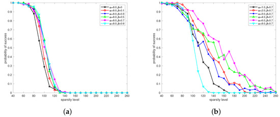
Figure 1. Comparison of the success rates of SPR-HBHTP with different parameters. (a) Different momentum coefficients $\beta$. (b) Different stepsizes $\alpha$.

4.2. Phase Transition

In this section, we use the phase transition curve (PTC) [42,43] and grayscale map to compare the recovery capabilities of the algorithms.

4.2.1. Phase Transition Curves

The phase transition curve is a logistic regression curve identifying a 50% success rate for the given algorithms in this paper. Indeed, a ratio of 50% can be replaced by other values in the interval $(0,1)$ based on the practical background. Denote $\delta =m/n$ and $\rho =s/m.$ The $(\delta ,\rho )$-plane is separated by the PTC of an algorithm into success and failure regions (see Figure 2). The former corresponds to the region below the PTC, wherein the algorithm can reconstruct the target sparse signal successfully; the latter corresponds to the region above the PTC. In other words, the higher the PTC, the stronger the recovery capability of the algorithm.

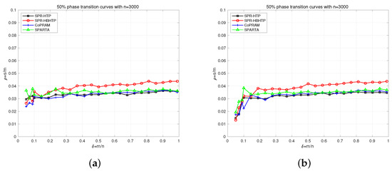
Figure 2. Comparison of the PTCs for the algorithms with accurate/inaccurate measurements. (a) Accurate measurements. (b) Inaccurate measurements with $\kappa$ = 0.01.

To generate the PTC, $(\delta ,\rho )$ are taken as follows

$$\begin{array}{c}\hfill \delta \in \left\{0.05,0.07,0.09,0.1,0.1445,\dots ,0.99\right\},\rho =s/m,\end{array}$$

(49)

where the interval $[0.1,0.99]$ is equally divided into 20 parts. For each $\delta$ given in (49), the ‘glmfit’ function in Matlab is used to generate the logistic regression curve based on the success rates with different sparsity levels s. The PTC is obtained directly by identifying the point in the logistic regression curve with a 50% success rate. This technique is almost the same as that shown in [36], except that the ‘glmfit’ function is replaced by the logistic regression model. Thus, the process of the generation of the PTC is omitted here, and the interested reader can consult [36] for detailed information.

The comparison of the PTCs for algorithms including SPR-HBHTP, SPR-HTP, CoPRAM, and SPARTA is shown in Figure 2, wherein Figure 2a,b correspond to accurate and inaccurate measurements, respectively. From Figure 2a, we see that SPR-HBHTP has the highest PTC as $\delta >0.2$, which indicates that the recovery capability of SPR-HBHTP is stronger than that of the other three algorithms, especially for larger $\delta$. The PTCs in Figure 2b are similar to those in Figure 2a as $\delta >0.1$; that is, all algorithms are stable under small disturbances. However, when $\delta \le 0.1$, all PTCs in Figure 2b decrease rapidly with a decrease in $\delta$, which is different from the phenomena shown in Figure 2a. This indicates that all algorithms require more measurements to ensure the recovery effect under the disturbance for the sparse phase retrieval problem. Finally, it should be noted that the PTCs of SPR-HTP, CoPRAM, and SPARTA are close to each other in Figure 2a,b, which means that the reconstruction capability of these three algorithms is almost the same. Comparatively speaking, the recovery capability of SPR-HTP is slightly better than those of CoPRAM and SPARTA.

4.2.2. Greyscale Maps

A grayscale map is an image that contains only brightness information and does not contain color information. In grayscale maps, the successful recovery rate of the algorithms is expressed by the different gray levels of the corresponding blocks, where black indicates a successful recovery rate of 0%, white is 100%, and gray is 0% to 100%.

Grayscale maps for different algorithms, such as SPR-HBHTP, SPR-HTP, CoPRAM and SPARTA, with signal lengths of n = 3000 are displayed in Figure 3. In our experiments, the sample size m ranged from 250 to 3000 with a stepsize of 250 and the sparsity s ranged from 20 to 100 with a stepsize of 5. By comparing the four graphs in Figure 3, it can be seen that when the sparsity is relatively large, the recovery ability of SPR-HBHTP is stronger than that of other algorithms. For smaller sparsity s values, SPR-HTP and CoPRAM have almost the same recovery ability, and similarly, SPARTA and SPR-HBHTP have comparable recovery abilities. This is consistent with our results for phase transition curves.

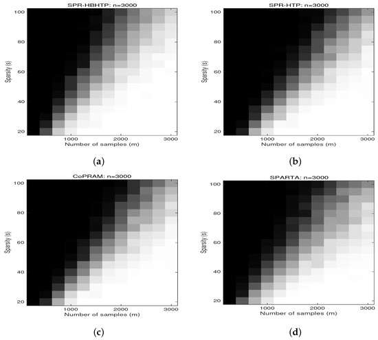
Figure 3. Grayscale map for different algorithms with n = 3000. (a) SPR-HBHTP. (b) SPR-HTP. (c) CoPRAM. (d) SPARTA.

4.3. Algorithm Selection Maps

In practice, the algorithm that consumes the least amount of time should be selected naturally when more than one algorithm can reconstruct the target signal successfully. Hence, it is meaningful to choose the fastest algorithm at the intersection of the success regions of the algorithms, which builds the algorithm selection maps (ASM) proposed in [42,43]. Note that the algorithm will be selected automatically if it is the only one that can recover the signal successfully.

Denote $\delta =m/n$ and $\rho =s/m.$ Next, we establish the ASM in the $(\delta ,\rho )$-plane with $(\delta ,\rho )$ given as follows

$$\begin{array}{c}\hfill \delta \in \left\{0.05,0.07,0.09,0.1,0.1445,\dots ,0.99\right\},\rho \in \left\{0.02,0.022,\dots ,0.1\right\},\end{array}$$

where the intervals $[0.1,0.99]$ and $[0.02,1]$ are equally divided into 20 and 40 parts, respectively. For each $\delta$, we tested 10 problem instances at $(\delta ,\rho )$ for each algorithm with an increase in $\rho$ until the success frequency was less than 50%. The ASM and average runtime of the fastest algorithm with accurate measurements are summarized in Figure 4. Figure 4a indicates that SPR-HBHTP or SPR-HTP is the fastest algorithm in most areas, and CoPRAM is a slower algorithm relatively, since it does not appear in the ASM. Figure 4b shows us that the average runtime of the fastest algorithm is less than one second in most regions, and it increases by up to 3–7 s for larger $\delta$ and $\rho$. This demonstrates that all algorithms will take more time, as the sparsity level s becomes larger.

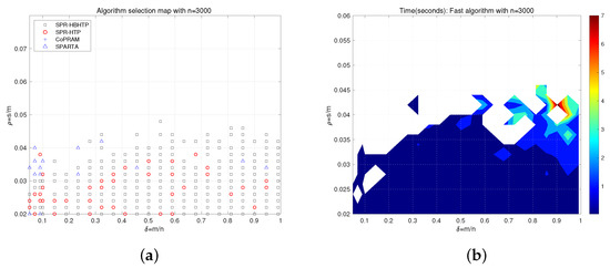
Figure 4. ASM and the shortest average runtime with accurate measurements. (a) ASM. (b) Average runtime of the fastest algorithm.

For comparing the algorithms thoroughly, we collected detailed information about their average runtimes, as shown in Figure 5, and the ratios of the average runtimes for the algorithms against the fastest one are shown in Figure 4b. Figure 5a,b reveal that the ratios of SPR-HBHTP and SPR-HTP are close to 1 in most areas, which indicates that they are faster than CoPRAM and SPARTA. In particular, the advantage value of SPR-HBHTP lies in the region with a larger $\rho$ compared to SPR-HTP. In Figure 5c, the ratio of CoPRAM is about 5–20 in most regions, and the minimum value is 5, which means that it is slower than the other three algorithms. Finally, by comparing Figure 5d with Figure 5a–c, we find that SPARTA is slower than SPR-HBHTP and SPR-HTP in most cases, but it is much faster than CoPRAM.

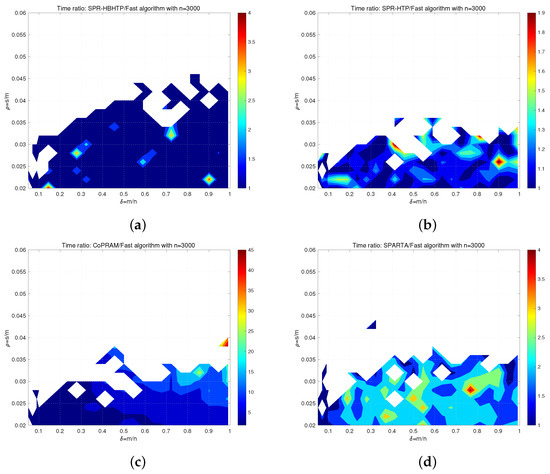
Figure 5. The ratios of average runtimes for the algorithms against the fastest one. (a) SPR-HBHTP. (b) SPR-HTP. (c) CoPRAM. (d) SPARTA.

5. Conclusions

We introduced a second-order accelerated method for the Hard Thresholding Pursuit, named the Heavy-Ball-Based Hard Thresholding Pursuit, to reconstruct a sparse signal from phaseless measurements. Under the restricted isometry property, SPR-HBHTP enjoys an exact provable recovery in the finite steps as soon as the number of noiseless Gaussian measurements exceeds a certain bound. It is remarkably different from the existing phase recovery algorithms in terms of theoretical analysis. Moreover, numerical experiments on random problem instances indicate that our algorithm outperforms the state-of-the-art algorithms, such as SPR-HTP, CoPRAM, and SPARTA, in terms of its recovery success rate and computational times through the phase transition analysis. Conducting experiments on realistic situations to truly verify the practical performance of SPR-HBHTP is worthy of further research. In addition, studying the random alternating minimization method based on Heavy-Ball acceleration is an interesting research topic.

References

- Shechtman, Y.; Eldar, Y.C.; Cohen, O.; Chapman, H.N.; Miao, J.W.; Segev, M. Phase retrieval with application to optical imaging: A contemporary overview. IEEE Signal Process Mag. 2015, 32, 87–109. [Google Scholar] [CrossRef]
- Gerchberg, R.; Saxton, W. A practical algorithm for the determination of plane from image and diffraction pictures. Optik 1972, 35, 237–246. [Google Scholar]
- Fienup, J.R. Phase retrieval algorithms: A comparison. Appl. Opt. 1982, 21, 2758–2769. [Google Scholar] [CrossRef] [PubMed]
- Marchesini, S. Phase retrieval and saddle-point optimization. J. Opt. Soc. Am. A 2007, 24, 3289–3296. [Google Scholar] [CrossRef] [PubMed]
- Nugent, K.; Peele, A.; Chapman, H.; Mancuso, A. Unique phase recovery for nonperiodic objects. Phys. Rev. Lett. 2003, 91, 203902. [Google Scholar] [CrossRef] [PubMed]
- Fickus, M.; Mixon, D.G.; Nelson, A.A.; Wan, Y. Phase retrieval from very few measurements. Linear Algebra Appl. 2014, 449, 475–499. [Google Scholar] [CrossRef]
- Chen, P.; Fannjiang, A.; Liu, G.R. Phase retrieval with one or two diffraction patterns by alternating projections with the null initialization. J. Fourier Anal. Appl. 2018, 24, 719–758. [Google Scholar] [CrossRef]
- Waldspurger, I. Phase retrieval with random gaussian sensing vectors by alternating projections. IEEE Trans. Inf. Theory 2018, 64, 3301–3312. [Google Scholar] [CrossRef]
- Candès, E.J.; Strohmer, T.; Voroninski, V. Phaselift: Exact and stable signal recovery from magnitude measurements via convex programming. Commun. Pure Appl. Math. 2013, 66, 1241–1274. [Google Scholar] [CrossRef]
- Waldspurger, I.; d’Aspremont, A.; Mallat, S. Phase recovery, maxcut and complex semidefinite programming. Math. Program. 2015, 149, 47–81. [Google Scholar] [CrossRef]
- Goldstein, T.; Studer, C. Phasemax: Convex phase retrieval via basis pursuit. IEEE Trans. Inf. Theory 2018, 64, 2675–2689. [Google Scholar] [CrossRef]
- Hand, P.; Voroninski, V. An elementary proof of convex phase retrieval in the natural parameter space via the linear program PhaseMax. Commun. Math. Sci. 2018, 16, 2047–2051. [Google Scholar] [CrossRef]
- Candès, E.J.; Li, X.; Soltanolkotabi, M. Phase retrieval via wirtinger flow: Theory and algorithms. IEEE Trans. Inf. Theory 2015, 61, 1985–2007. [Google Scholar] [CrossRef]
- Netrapalli, P.; Jain, P.; Sanghavi, S. Phase retrieval using alternating minimization. IEEE Trans. Signal Process 2015, 18, 4814–4826. [Google Scholar] [CrossRef]
- Cai, J.F.; Li, J.; Lu, X.; You, J. Sparse signal recovery from phaseless measurements via hard thresholding pursuit. Appl. Comput. Harmon. Anal. 2022, 56, 367–390. [Google Scholar] [CrossRef]
- Cai, J.F.; Jiao, Y.L.; Lu, X.L.; You, J.T. Sample-efficient sparse phase retrieval via stochastic alternating minimization. IEEE Trans. Signal Process 2022, 70, 4951–4966. [Google Scholar] [CrossRef]
- Yang, M.H.; Hong, Y.W.P.; Wu, J.Y. Sparse affine sampling: Ambiguity-free and efficient sparse phase retrieval. IEEE Trans. Inf. Theory 2022, 68, 7604–7626. [Google Scholar] [CrossRef]
- Bakhshizadeh, M.; Maleki, A.; Jalali, S. Using black-box compression algorithms for phase retrieval. IEEE Trans. Inf. Theory 2020, 66, 7978–8001. [Google Scholar] [CrossRef]
- Cha, E.; Lee, C.; Jang, M.; Ye, J.C. DeepPhaseCut: Deep relaxation in phase for unsupervised fourier phase retrieval. IEEE Trans. Pattern. Anal. Mach. Intell. 2022, 44, 9931–9943. [Google Scholar] [CrossRef]
- Wang, B.; Fang, J.; Duan, H.; Li, H. PhaseEqual: Convex phase retrieval via alternating direction method of multipliers. IEEE Trans. Signal Process 2020, 68, 1274–1285. [Google Scholar] [CrossRef]
- Liu, T.; Tillmann, A.M.; Yang, Y.; Eldar, Y.C.; Pesavento, M. Extended successive convex approximation for phase retrieval with dictionary learning. IEEE Trans. Signal Process 2022, 70, 6300–6315. [Google Scholar] [CrossRef]
- Fung, S.W.; Di, Z.W. Multigrid optimization for large-scale ptychographic phase retrieval. SIAM J. Imaging Sci. 2020, 13, 214–233. [Google Scholar] [CrossRef]
- Chen, Y.; Chi, Y.; Fan, J.; Ma, C. Gradient descent with random initialization: Fast global convergence for nonconvex phase retrieval. Math. Program. 2019, 176, 5–37. [Google Scholar] [CrossRef]
- Cai, J.F.; Huang, M.; Li, D.; Wang, Y. Solving phase retrieval with random initial guess is nearly as good as by spectral initialization. Appl. Comput. Harmon. Anal. 2022, 58, 60–84. [Google Scholar] [CrossRef]
- Soltanolkotabi, M. Structured signal recovery from quadratic measurements: Breaking sample complexity barriers via nonconvex optimization. IEEE Trans. Inf. Theory 2019, 65, 2374–2400. [Google Scholar] [CrossRef]
- Jaganathan, K.; Oymak, S.; Hassibi, B. Sparse phase retrieval: Uniqueness guarantees and recovery algorithms. IEEE Trans. Signal Process. 2017, 65, 2402–2410. [Google Scholar] [CrossRef]
- Killedar, V.; Seelamantula, C.S. Compressive phase retrieval based on sparse latent generative priors. In Proceedings of the ICASSP 2022—2022 IEEE International Conference on Acoustics, Speech and Signal Processing (ICASSP), Singapore, 23–27 May 2022; pp. 1596–1600. [Google Scholar]
- Wen, J.; He, H.; He, Z.; Zhu, F. A pseudo-inverse-based hard thresholding algorithm for sparse signal recovery. IEEE Trans. Intell. Transp. Syst. 2022. [Google Scholar] [CrossRef]
- Foucart, S. Hard thresholding pursuit: An algorithm for compressive sensing. SIAM J. Numer. Anal. 2011, 49, 2543–2563. [Google Scholar] [CrossRef]
- Foucart, S.; Rauhut, H. An Invitation to Compressive Sensing. In A Mathematical Introduction to Compressive Sensing; Springer: Berlin/Heidelberg, Germany, 2013; pp. 1–39. [Google Scholar]
- Blumensath, T.; Davies, M.E. Iterative hard thresholding for compressed sensing. Appl. Comput. Harmon. Anal. 2009, 27, 265–274. [Google Scholar] [CrossRef]
- Tropp, J.A.; Gilbert, A.C. Signal recovery from random measurements via orthogonal matching pursuit. IEEE Trans. Inf. Theory 2007, 53, 4655–4666. [Google Scholar] [CrossRef]
- Needell, D.; Tropp, J. CoSaMP: Iterative signal recovery from incomplete and inaccurate samples. Appl. Comput. Harmon. Anal. 2009, 26, 301–321. [Google Scholar] [CrossRef]
- Dai, W.; Milenkovic, O. Subspace pursuit for compressive sensing signal reconstruction. IEEE Trans. Inf. Theory 2009, 55, 2230–2249. [Google Scholar] [CrossRef]
- Polyak, B.T. Some methods of speeding up the convergence of iteration methods. Comp. Math. Math. Phys. 1964, 4, 1–17. [Google Scholar] [CrossRef]
- Sun, Z.F.; Zhou, J.C.; Zhao, Y.B.; Meng, N. Heavy-ball-based hard thresholding algorithms for sparse signal recovery. J. Comput. Appl. Math. 2023, 430, 115264. [Google Scholar] [CrossRef]
- Candès, E.J. The restricted isometry property and its implications for compressed sensing. Crendus. Math. 2008, 346, 589–592. [Google Scholar] [CrossRef]
- Wang, G.; Zhang, L.; Giannakis, G.B.; Akçakaya, M.; Chen, J. Sparse phase retrieval via truncated amplitude flow. IEEE Trans. Signal Process 2018, 66, 479–491. [Google Scholar] [CrossRef]
- Jagatap, G.; Hegde, C. Sample-efficient algorithms for recovering structured signals from magnitude-only measurements. IEEE Trans. Inf. Theory 2019, 65, 4434–4456. [Google Scholar] [CrossRef]
- Cai, T.T.; Li, X.; Ma, Z. Optimal rates of convergence for noisy sparse phase retrieval via thresholded wirtinger flow. Ann. Stat. 2016, 44, 2221–2251. [Google Scholar] [CrossRef]
- Zhao, Y.B. Optimal k-thresholding algorithms for sparse optimization problems. SIAM J. Optim. 2020, 30, 31–55. [Google Scholar] [CrossRef]
- Blanchard, J.D.; Tanner, J. Performance comparisons of greedy algorithms in compressed sensing. Numer. Linear Algebra Appl. 2015, 22, 254–282. [Google Scholar] [CrossRef]
- Blanchard, J.D.; Tanner, J.; Wei, K. CGIHT: Conjugate gradient iterative hard thresholding for compressed sensing and matrix completion. Inf. Inference 2015, 4, 289–327. [Google Scholar] [CrossRef]
Disclaimer/Publisher’s Note: The statements, opinions and data contained in all publications are solely those of the individual author(s) and contributor(s) and not of MDPI and/or the editor(s). MDPI and/or the editor(s) disclaim responsibility for any injury to people or property resulting from any ideas, methods, instructions or products referred to in the content. |
© 2023 by the authors. Licensee MDPI, Basel, Switzerland. This article is an open access article distributed under the terms and conditions of the Creative Commons Attribution (CC BY) license (https://creativecommons.org/licenses/by/4.0/).