Analysis of Drag Coefficients around Objects Created Using Log-Aesthetic Curves

Abstract

A fair curve with exceptional properties, called the log-aesthetic curves (LAC) has been extensively studied for aesthetic design implementations. However, its implementation in terms of functional design, particularly hydrodynamic design, remains mostly unexplored. This study examines the effect of the shape parameter $\alpha$ of LAC on the drag generated in an incompressible fluid flow, simulated using a semi-implicit backward difference formula coupled with P${}_2$−P${}_1$ Taylor–Hood finite elements. An algorithm was developed to create LAC hydrofoils that were used in this study. We analyzed the drag coefficients of 47 LAC hydrofoils of three sizes with various shapes in fluid flows with Reynolds numbers of 30, 40, and 100, respectively. We found that streamlined LAC shapes with negative $\alpha$ values, of which curvature with respect to turning angle are almost linear, produce the lowest drag in the incompressible flow simulations. It also found that the thickness of LAC objects can be varied to obtain similar drag coefficients for different Reynolds numbers. Via cluster analysis, it is found that the distribution of drag coefficients does not rely solely on the Reynolds number, but also on the thickness of the hydrofoil.

1. Introduction

Log-aesthetic curve (LAC), first proposed by Yoshimoto and Harada [1], refers to a family of aesthetically pleasing curves with monotonic curvatures. Harada et al. [2] found that the manufactured and natural shapes that are deemed beautiful have a linear Logarithmic Distribution Diagram of Curvature (LDDC). Thus, Miura [3] derived the LAC fundamental equation by equating the gradient of the Logarithmic Curvature Graph (LCG), the analytical form of LDDC, to a constant $\alpha$, which is the parameter determining the shape of the LAC. A designer usually interrogates curves using the curvature profiles, which involve second derivatives of curves, whereas LCG involves third derivatives, which are thus suitable for higher-order shape interrogation [4].

LAC has since then been proposed for many applications such as car design [5], modeling transitional curves [6], path planning [7], Computer-Aided Design (CAD) systems [8], and architecture design [9]. The success of LAC is due to its underlying properties; it has a sufficient degree of freedom and shape parameters to represent various spirals [10]. However, there is still much to be discovered about its fluid dynamics properties. It is unknown how fluid flow and drag changes with the change in the LAC’s shape, which is determined by its shape parameter $\alpha$. To the best of our knowledge, there is not yet any literature that elucidates this relationship.

Takuma et al. [11] studied how curvature affects the energy absorption characteristic of cylindrical corrugated tubes, showing that curve properties such as curvature have more to offer than contributing solely to aesthetic appeals. Likewise, we wish to elucidate how LACs’ shape properties, e.g., LCG gradient and curvature, affect fluid dynamics of incompressible fluid flows. Hence, we constructed hydrofoil-like objects using LAC and investigated their drag coefficient in an incompressible fluid flow using numerical simulation. The information obtained from this study may aid in designing submerged structures, objects, or vehicles, especially in drag reduction.

Lift and drag evaluations were based on the volume integral formulation found in [12,13]. The volume integral formulation has been known to provide better lift and drag coefficient estimations than conventional line integrals along our streamlined-shaped object. Furthermore, volume integral formulation is known to be less sensitive to a slight change in the mesh generated around the object. Recently, [14] reported the behavior of streamlines and fluid flow around streamlined-shaped objects constructed with LAC.

The contribution of this paper is two-fold. This paper completes the work of Wo et al. [14] to report how an LAC’s shape, dictated by its shape parameter, influences the drag of an incompressible fluid flow. An effect of the Reynolds number on the drag coefficient trend is also observed. Furthermore, an algorithm was developed to create LAC that satisfies given length, height, $G^1$ Hermite data on one end, and $G^0$ Hermite data on the other. This algorithm is used to construct LAC hydrofoils used in this study.

The rest of the paper is organized as follows. Section 2 discusses the numerical method used to simulate the incompressible non-stationary fluid flow. Section 3 elucidates the creation of an LAC hydrofoil with user-specified thickness and shape parameter $\alpha$. Section 4 specifies the computational and domain settings used for the simulations. The simulation results and their drag coefficient distribution are presented and discussed in Section 5 and Section 6, respectively. Finally, a conclusion is made, and future work is briefly discussed at the end of this paper. The results are expected to serve as a stepping stone in preparing LACs for hydrodynamic design.

2. Modeling Incompressible Fluid Flow and the Drag Coefficient

To solve an incompressible two-dimensional fluid flow problem using a numerical scheme, we first rewrite the Navier–Stokes Equation (NSE) in its weak formulation form [13]:

$$\begin{array}{c}\hfill \begin{array}{cc}\hfill \frac{\partial u}{\partial t}+u·\nabla u-\nu \Delta u+\frac{1}{\rho }\nabla p& =f\mathrm{on}\Omega \times (0,\mathbf{T}),\hfill \\ \hfill \nabla ·u& =0\mathrm{on}\Omega \times (0,\mathbf{T}),\hfill \\ \hfill u(x,0)& =u_0\mathrm{in}\Omega ,\hfill \\ \hfill u(x,t)& =g\mathrm{on}\Gamma \times (0,\mathbf{T}),\hfill \end{array}\end{array}$$

(1)

where u is the velocity vector field, $\nu$ is the kinematic viscosity, p is the pressure, f represents any external force (which is usually zero), $u_0$ is the initial velocity, $\mathbf{T}$ is the maximum time (t), and g is the condition (velocity field) enforced on the boundary $\Gamma$ of domain $\Omega$. The additional f in the equation will not affect any of the subsequent analyses [15]. We set $\rho =1$ and assume the effect of gravity is negligible for the problem.

We choose the Finite Element Method (FEM) for the space approximation of NSE. The semi-discrete form for Equation (1) is given as follows:

$$\begin{array}{c}\hfill {\int }_{\Omega }\frac{d}{dt}{\mathbf{u}}_{\widehat{h}}\left(t\right)·{\mathbf{v}}_{\widehat{h}}d\mathbf{x}+{\int }_{\Omega }\nu \nabla {\mathbf{u}}_{\widehat{h}}\left(t\right):\nabla {\mathbf{v}}_{\widehat{h}}d\mathbf{x}+{\int }_{\Omega }\left({\mathbf{u}}_{\widehat{h}}\left(t\right)·\nabla {\mathbf{u}}_{\widehat{h}}\left(t\right)\right)·{\mathbf{v}}_{\widehat{h}}d\mathbf{x}\\ \hfill -{\int }_{\Omega }{p}_{\widehat{h}}\left(t\right)\nabla ·{\mathbf{v}}_{\widehat{h}}d\mathbf{x}={\int }_{\Omega }{f}_{\widehat{h}}\left(t\right)·{\mathbf{v}}_{\widehat{h}}d\mathbf{x},\forall {\mathbf{v}}_{\widehat{h}}\in V_{\widehat{h}},\end{array}$$

(2)

$$\begin{array}{r}\hfill -{\int }_{\Omega }{q}_{\widehat{h}}\nabla ·{\mathbf{u}}_{\widehat{h}}\left(t\right)d\mathbf{x}=0,\forall q_{\widehat{h}}\in M_{\widehat{h}},\end{array}$$

(3)

$$\begin{array}{c}\hfill {\mathbf{u}}_{\widehat{h}}\left(0\right)={\mathbf{u}}_{\widehat{h}}^0,\end{array}$$

(4)

where ${\mathbf{u}}_{\widehat{h}}^0$ is an approximation of $u_0$ [13]. Our goal is to find ${\mathbf{u}}_{\widehat{h}}$$\left(t\right)\in V_{\widehat{h}}$ and $p_{\widehat{h}}\left(t\right)\in M_{\widehat{h}}$ for all $t\in (0,\mathbf{T})$. We follow the standard notation for Sobolev spaces for the rest of this paper [16]. Using the Taylor–Hood discretization of space, the following spaces are obtained [13]:

$$\begin{array}{c}\hfill \begin{array}{c}\hfill V_{\widehat{h}}=X_{\widehat{h}}\cap {\left[H_0^1\left(\Omega \right)\right]}^2,X_{\widehat{h}}=\left\{{\mathbf{v}}_{\widehat{h}}\in {\left[{\mathbb{C}}^0\left(\overline{\Omega }\right)\right]}^2|{\mathbf{v}}_{\widehat{h}|K}\in {\mathbb{P}}_2,\forall K\in T_{\widehat{h}}\right\},\\ \hfill M_{\widehat{h}}=Y_{\widehat{h}}\cap L_0^2\left(\Omega \right),Y_{\widehat{h}}=\left\{q_{\widehat{h}}\in {\mathbb{C}}^0\left(\overline{\Omega }\right)|q_{\widehat{h}|K}\in {\mathbb{P}}_1,\forall K\in T_{\widehat{h}}\right\},\end{array}\end{array}$$

(5)

where $q_{\widehat{h}}$ is a continuous function, $⟨p_{\widehat{h}},q_{\widehat{h}}⟩={\int }_{\Omega }{p}_{\widehat{h}}{q}_{\widehat{h}}d\Omega$, and $\parallel q_{\widehat{h}}{\parallel }_0={⟨q_{\widehat{h}},q_{\widehat{h}}⟩}^{\frac{1}{2}}$. The notation $H_0^1$ denotes the subset of the Sobolev space $H^1$ (of functions with at least one weak derivative), whose members are equal to zero at the boundaries of the domain. Meanwhile, ${\mathbb{C}}^0$ denotes the space of continuous functions defined in $\Omega$.

The Taylor–Hood elements satisfy the inf-sup condition, also known as the Ladyzhenskaya–Babuška–Brezzi condition (LBB), indicating that the system is well-posed [17,18]. The Taylor–Hood elements consist of continuous piece-wise quadratic polynomials for velocity and linear polynomials for pressure (see Figure 1). The notation $T_{\widehat{h}}$ represents a regular triangulation of $\Omega$, while ${\mathbb{P}}_k$ denotes the Lagrange polynomials space of k-degree on the triangles K. The pressure, p, is taken into $L_0^2$ ($\Omega$) for both Stokes equation and NSE. The notation $L_0^2$ ($\Omega$) stands for the space of (generalized) functions $L^2$ ($\Omega$), which are square-integrable and have a zero average on $\Omega$ [13,19]. This is because p is only unique up to a constant when the velocity’s Dirichlet boundary condition is imposed on all $\partial \Omega$. To counter this, we penalize the pressure to restrain the constant such that a non-singular algebraic system can be acquired [13]. The solution ($u_{\epsilon }$,$p_{\epsilon }$), where $\epsilon >0$ is the penalized parameter, produced by the penalized system, converges to the non-penalized system’s $(u,p)$ [20].

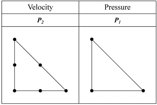
Figure 1. Conventional representation of the Taylor–Hood ${\mathit{P}}_2-{\mathit{P}}_1$ element.

The application of the second-order semi-implicit time-stepping method onto the NSE can produce the following problem [13]: given values ${\left\{u^j\right\}}_{j=0}^1$ and a constant time step, $\Delta t$, find the solution $(u^{n+2},p^{n+2})$ of

$$\begin{array}{c}\hfill \begin{array}{c}\hfill \stackrel{\mathrm{The}\mathrm{discretization}\mathrm{of}\mathrm{time}\mathrm{derivative}}{\overbrace{\frac{1}{\Delta t}\left(\alpha {\mathbf{u}}^{n+2}+\sum _{j=i}^k{\beta }_j{u}^{n+2-j}\right)}}-\nu \Delta {\mathbf{u}}^{n+2}+\stackrel{\mathrm{Nonlinear}\mathrm{advection}\mathrm{extrapolated}\mathrm{at}\mathrm{t} = {\mathrm{t}}^{\mathrm{n}+2}}{\overbrace{\sum _{j=1}^k{\gamma }_j{\mathbf{u}}^{n+2-j}·\nabla {\mathbf{u}}^{n+2-j}}}\\ \hfill +\nabla p^{n+2}={\mathbf{f}}^{n+2}.\end{array}\end{array}$$

(6)

The coefficients $\alpha ,{\left\{{\beta }_j\right\}}_{j=1}^2\in \mathbb{R}$, where $\mathbb{R}$ represents real numbers, are the result of applying the backward differentiation formula on the time derivative with $\alpha +{\sum }_{j=1}^2{\beta }_j=0$. Meanwhile, the coefficients ${\left\{{\gamma }_j\right\}}_{j=1}^2\in \mathbb{R}$ generate the extrapolation formula for the nonlinear term, which satisfies ${\sum }_{j=1}^2{\gamma }_j=0$. The terms $\nabla p^{n+2}$ and $\nabla ·u^{n+2}$ used in the velocity–pressure coupling are taken implicitly to strictly enforce the discrete incompressibility condition. The diffusion term $-\nabla u^{n+2}$ is taken implicitly as well, to prevent stringent stability conditions in $O\left({\nu }^{-1}{\widehat{h}}^2\right)$ on the time step.

This study employs the second-order semi-implicit backward difference formula (SBDF) [13]. The SBDF does not self-start and hence requires a proper initialization for ${\left\{u_j\right\}}_{j=1}^2$, in other words, obtainin $u^1$ from $u^0$, which can be achieved by simply employing the first-order SBDF. The time-discretized momentum equation when second-order SBDF is applied is written as [13]: given the initial solution $u_h^0$ and a proper initialization, $u_{\widehat{h}}^1$, we can find the solution $(u_{\widehat{h}}^{n+2},p_{\widehat{h}}^{n+2})$ of

$$\frac{3{\mathbf{u}}_{\widehat{h}}^{n+2}-4{\mathbf{u}}_{\widehat{h}}^{n+1}+{\mathbf{u}}_{\widehat{h}}^n}{2\Delta t}-\nu \Delta {\mathbf{u}}_{\widehat{h}}^{n+2}+\nabla p_{\widehat{h}}^{n+2}={\mathbf{f}}_{\widehat{h}}^{n+2}-2B\left({\mathbf{u}}_{\widehat{h}}^{n+1}\right)+B\left({\mathbf{u}}_{\widehat{h}}^n\right),$$

(7)

for all $n\in \mathbb{N}$, where the nonlinear advection term is denoted by $B({\mathbf{u}}_{\widehat{h}})={\mathbf{u}}_{\widehat{h}}·\nabla {\mathbf{u}}_{\widehat{h}}$. The notation $\mathbb{N}$ denotes the set of natural numbers.

3. Creating Same-Sized LAC Hydrofoils with Various Shapes

The hydrofoils are generated using the LAC Equation [21]:

$$P\left(\theta \right)=\left\{\begin{array}{cc}{\int }_0^{\theta }{e}^{(\Lambda +i)\psi }d\psi ,\hfill & \mathrm{if}\alpha =1\hfill \\ {\int }_0^{\theta }{((\alpha -1)\Lambda \psi +1)}^{\frac{1}{\alpha -1}}{e}^{\psi i}d\psi ,\hfill & \mathrm{otherwise}\hfill \end{array}\right.$$

(8)

where $\alpha$ dictates the type and shape of the LAC generated, $\Lambda$ is the rate of change of curvature with respect to the curve’s arc length, and $\theta$ is the turning angle of the curve. It is well known that LACs with $\alpha =-1$, 0, and 1 are the Euler spiral, logarithmic spiral, and Nielsen’s spiral, respectively. LACs with $\alpha <0$ are curves classified as divergent, $\alpha =0$ as neutral, and $\alpha >0$ as convergent. These classifications are based on the designers’ impression of the curve [22].

The hydrofoils used in this study were generated using Equation (8) by fixing the length (c) and height of the LAC, which makes up the upper half of the hydrofoil, through manipulating $\Lambda$ and scaling the LAC while ensuring the tangent vector ($\overrightarrow{T}$) at the leading edge is orthogonal to the x-axis (see Figure 2). The generated curve is then reflected along the x-axis to produce the complete hydrofoil shape. The generated shape is $G^2$-continuous everywhere except at the trailing edge [23]. The thickness of the thickest section of the hydrofoil is denoted by h.

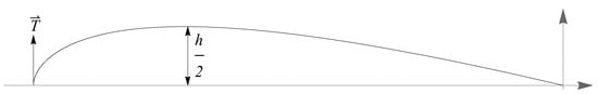
Figure 2. An LAC that makes up half of the hydrofoil.

The steps for generating the hydrofoils are elucidated in Algorithm 1. Two examples of the output are shown in Figure 3 and Figure 4. The size difference in the figure refers to the difference between the size of the LAC of the input $\alpha$ value (orange) and the size of the LAC of $\alpha =0$ (grey).

Algorithm 1 Building LAC Hydrofoil with User-specified Size

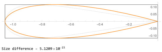
Figure 3. Example output of Algorithm 1 (input $\alpha =0.75$).

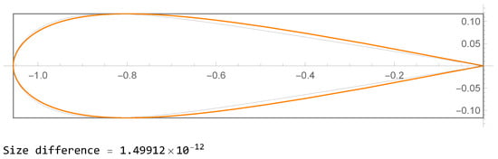
Figure 4. Example output of Algorithm 1 (input $\alpha =0.25$).

4. Simulation and Domain Settings

The simulation domain comprises a rectangular boundary and the boundary of the hydrofoil-shaped object in it. The rectangular boundary has vertices $(-12.5,-12.5)$, $(-12.5,12.5)$, $(21,12.5)$, and $(21,-12.5)$. This is $33.5$ times the chord length, c, of the LAC hydrofoil in length and 25 times c in height to ensure a sufficiently accurate simulation and drag coefficient computation [24,25]. The leading edge of the hydrofoil is set at $(-1.05551,0)$, and the trailing edge at $(0,0)$.

The boundary conditions for the rectangular boundary’s edges ($L_1$, $L_2$, $L_3$, $L_4$) and the hydrofoil ($L_5$) are shown in Figure 5. Each meshed domain has approximately 75,000 nodes. The maximum mesh spacing is 0.6 units on the rectangular boundary. The minimum mesh spacing is approximately 0.0004 units on the LAC hydrofoil. The meshed domain is illustrated in Figure 6. FreeFem++ [26] was employed to solve the incompressible Navier–Stokes equations. The space approximation was carried out using the Taylor–Hood finite element (${\mathit{P}}_2-{\mathit{P}}_1$) while a second-order semi-implicit backward difference formula was chosen for time integration. The combined method provides fairly accurate approximations for both velocity and pressure [13]. The drag coefficients are then recorded upon reaching a steady state or when the first derivative for velocity with respect to time (in the Navier–Stokes equation) is less than ${10}^{-5}$.

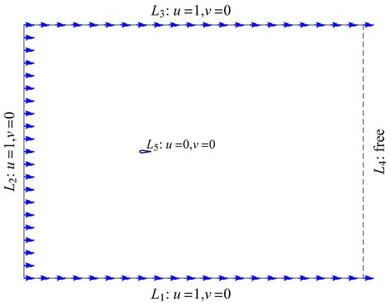
Figure 5. FEM domain with the LAC hydrofoil ($\alpha =1$) and boundary conditions.

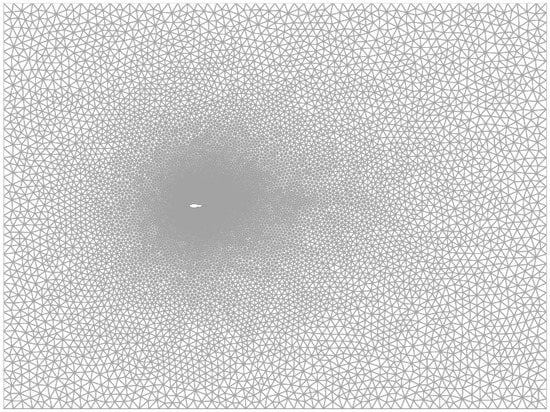
Figure 6. Meshed FEM domain with the LAC hydrofoil ($\alpha =0.5$).

Three experiments (cases) were designed in which the hydrofoils had different thicknesses at the thickest section of the hydrofoil-shaped object. The objects’ thickness h for Case 1, Case 2, and Case 3 are 0.234185, 0.3, and 0.4, respectively. In each case, the flow is simulated around hydrofoils with the same maximum thickness but different $\alpha$ values to find their drag coefficients $C_D$. These hydrofoils have different shapes and leading-edge curvatures (see Figure 7, Figure 8 and Figure 9). The $\alpha$ values of the hydrofoils in Figure 7 (Case 1) are {−0.05, −0.025, −0, 0.05, 0.1, 0.15, 0.2, 0.25, 0.3, 0.4, 0.5, 0.6, 0.75, 0.8, 0.9, 1}. The hydrofoil with the smallest $\alpha$ value is colored in blue, and the color gradually changes into yellow as $\alpha$ increases. The $\alpha$ values of the hydrofoil in Figure 8 (Case 2) are {−0.05, 0, 0.05, 0.1, 0.15, 0.25, 0.3, 0.4, 0.5, 0.6, 0.75, 0.8, 0.9, 1, 1.2} whereas for Figure 9 (Case 3), they are {−0.25, −0.05, 0, 0.05, 0.1, 0.15, 0.25, 0.3, 0.4, 0.5, 0.6, 0.75, 0.8, 0.9, 1, 1.5}. Note that the LACs with $\alpha =0$ and $\alpha =1$ are also known as the Nielsen’s spiral and Logarithmic spiral, respectively [21]. We need to fulfill the $G^2$ data at the leading edge, the $G^0$ data at the trailing edge, and the thickness of the hydrofoil to generate the hydrofoil shapes. However, due to the lack of the single-segment LACs’ degree of freedom, we can only create profiles within a specific range of $\alpha$ in each case, thus resulting in the difference between the range of $\alpha$ values used in the three cases.

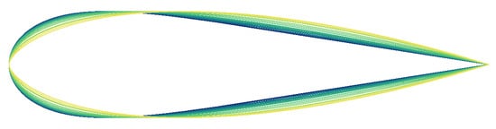
Figure 7. Comparison of Case 1 ($h=0.234185$) hydrofoil shapes from $\alpha =-0.05$ (blue) to $\alpha =1$ (yellow).

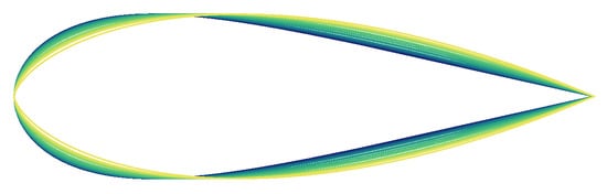
Figure 8. Comparison of Case 2 ($h=0.3$) hydrofoil shapes from $\alpha =-0.05$ (blue) to $\alpha =1.2$ (yellow).

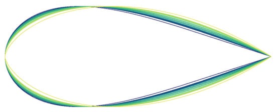
Figure 9. Comparison of Case 3 ($h=0.4$) hydrofoil shapes from $\alpha =-0.25$ (blue) to $\alpha =1.5$ (yellow).

Three simulations were run using different Reynolds numbers ($\mathrm{Re}$): 30, 40, and 100. While $\mathrm{Re}=30$ was chosen arbitrarily, the other two $\mathrm{Re}$ values were chosen to examine how the LAC hydrofoils’ drag coefficients change when there is a small increment in $\mathrm{Re}$, i.e., from 30 to 40, and a large increment from 40 to 100. It is also notable that at $\mathrm{Re}=100$, the fluid’s viscosity is similar to that of water at 20 degrees Celsius, assuming 1 unit equals 0.1 m. The flows are assumed to be laminar, meaning the streamlines were smooth and regular. The Reynolds number is a similarity parameter that measures the ratio of inertial forces to viscous forces in a flow [27]. The fluid at $\mathrm{Re}=100$ is deemed to produce less viscous flows than $\mathrm{Re}=30$ and 40. We ran nine sets of simulations comprising 141 individual simulations in total. The results are presented and discussed in the following section.

5. Results and Discussion

The drag coefficients denoted as $C_D$ for each simulation are listed in Table 1, Table 2 and Table 3 and plotted in Figure 10, Figure 11 and Figure 12. The difference between the lowest $C_D$ and the highest is shown on the right side of Figure 10, Figure 11 and Figure 12.

Table 1. $\alpha$ and $C_D$ for simulations with $\mathrm{Re}=30$.

$\mathit{\alpha }$	Case 1	Case 2	Case 3
−0.25	-	-	0.521258
−0.05	0.446640	0.475329	0.522634
−0.025	0.446800	-	-
0	0.446969	0.475734	0.522961
0.05	0.447340	0.476112	0.523232
0.1	0.447697	0.476487	0.523516
0.15	0.448072	0.476843	0.523750
0.2	0.448431	-	-
0.25	0.448761	0.477721	0.524190
0.3	0.449071	0.47815	0.524372
0.4	0.449556	0.478454	0.524683
0.5	0.449860	0.478641	0.524931
0.6	0.450000	0.47869	0.525093
0.75	0.449951	0.47866	0.525211
0.8	0.449783	0.478519	0.525236
0.9	0.449555	0.478327	0.525195
1	0.449168	0.477669	0.525139
1.2	-	0.475734	-
1.5	-	-	0.524178

Table 2. $\alpha$ and $C_D$ for simulations with $\mathrm{Re}=40$.

$\mathit{\alpha }$	Case 1	Case 2	Case 3
−0.25	-	-	0.448448
−0.05	0.37942	0.405816	0.449585
−0.025	0.379562	-	-
0	0.379712	0.406168	0.449856
0.05	0.380041	0.406495	0.450076
0.1	0.380358	0.406821	0.450311
0.15	0.38069	0.407127	0.450501
0.2	0.381008	-	-
0.25	0.381299	0.407885	0.450860
0.3	0.381575	0.408255	0.451006
0.4	0.382005	0.408515	0.451255
0.5	0.382276	0.408674	0.451452
0.6	0.382403	0.408714	0.451575
0.75	0.382372	0.408688	0.451655
0.8	0.382229	0.408566	0.451671
0.9	0.38204	0.408403	0.451623
1	0.381712	0.407844	0.451566
1.2	-	0.407665	-
1.5	-	-	0.450725

Table 3. $\alpha$ and $C_D$ for simulations with $\mathrm{Re}=100$.

$\mathit{\alpha }$	Case 1	Case 2	Case 3
−0.25	-	-	0.285798
−0.05	0.230045	0.250844	0.286243
−0.025	0.230138	-	-
0	0.230236	0.251051	0.286353
0.05	0.230454	0.251242	0.286429
0.1	0.230660	0.251431	0.286522
0.15	0.230879	0.251607	0.286585
0.2	0.231089	-	-
0.25	0.231278	0.251917	0.286711
0.3	0.231461	0.252042	0.286755
0.4	0.231748	0.252250	0.286825
0.5	0.231933	0.252394	0.286874
0.6	0.232026	0.252478	0.286883
0.75	0.232035	0.252487	0.286845
0.8	0.231950	0.252469	0.286833
0.9	0.231858	0.252392	0.286756
1	0.231678	0.252301	0.286686
1.2	-	0.251984	-
1.5	-	-	0.286111

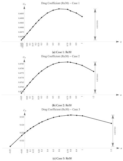
Figure 10. The drag coefficient of objects for various $\alpha$ values ($\mathrm{Re}=30$).

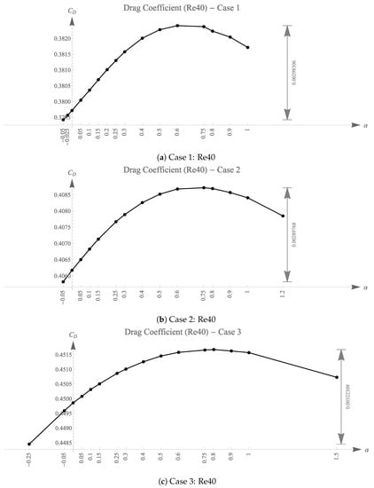
Figure 11. Drag coefficient of objects for various $\alpha$ values ($\mathrm{Re}=40$).

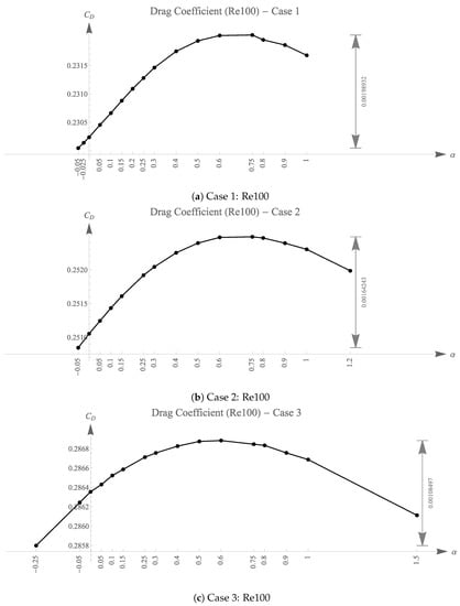
Figure 12. $C_D$ of objects for various $\alpha$ values ($\mathrm{Re}=100$).

It is observed that for each simulation of a different $\mathrm{Re}$, the $C_D$ values for shapes of different $\alpha$ exhibit a similar trend, as shown in Case 1 and Case 2. This is reflected in the sudden drop in $C_D$ values for shapes of $\alpha =0.8$. The $C_D$ values for these cases peaked around $\alpha =0.6$ to $\alpha =0.75$. However, for Case 3, the peak of the $C_D$ graph with $\mathrm{Re}=100$ shifted left, from $\alpha =0.8$ to $\alpha =0.6$, obviously deviating from the simulations with $\mathrm{Re}=30$ and $\mathrm{Re}=40$. The standardized $C_D$ graphs are plotted in Figure 13. The standardization shifts and rescaled $C_D$ values of LAC hydrofoils with the same thickness but different $\mathrm{Re}$ have zero mean and unit sample variance for better comparison of the $C_D$ trends. The $\alpha$ values of the LAC shape that creates the most drag are shown in Table 4, along with the corresponding $C_D$ values. The rate of change of the drag coefficient decreases as $\mathrm{Re}$ increases. This statement is true for Cases 1–3.

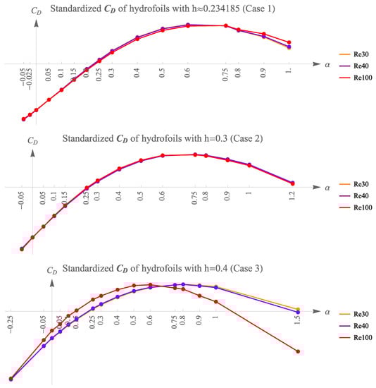
Figure 13. Comparison of the $C_D$ graph shape of all simulations.

Table 4. $\alpha$ values of the LAC shape that create the highest $C_D$ and the corresponding $C_D$.

	Case 1 ($\mathit{h}\approx 0.2$)		Case 2 ($\mathit{h}=0.3$)		Case 3 ($\mathit{h}=0.4$)
	$\mathbf{\alpha }$	${\mathit{C}}_{\mathit{D}}$	$\mathbf{\alpha }$	${\mathit{C}}_{\mathit{D}}$	$\mathbf{\alpha }$	${\mathit{C}}_{\mathit{D}}$
$\mathrm{Re}=30$	0.6	0.450000	0.75	0.478660	0.8	0.525236
$\mathrm{Re}=40$	0.6	0.382403	0.75	0.408688	0.8	0.451671
$\mathrm{Re}=100$	0.75	0.232035	0.75	0.252487	0.6	0.286883

The streamlines (flow lines), which show the local directions of the vector field of the simulations with the lowest and highest $C_D$ values at a steady state are shown in Figure 14, Figure 15 and Figure 16. The rainbow color in the background shows the scalar field, i.e., flow speed, with red indicating low speed and purple indicating higher speed. The detachment of a boundary layer from a surface is known as flow separation [28]. Flow separation is most apparent in the simulation of Case 3 with $\mathrm{Re}=100$. More separation is seen in the shape, which creates a more substantial drag. As such, most of the drag force is made up of skin friction drag. The possible onset of wakes or flow separation in the simulation of Case 3 ($\mathrm{Re}=100$) could be the reason for the change in the $C_D$ trend observed earlier.

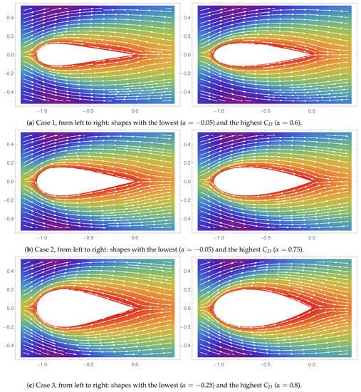
Figure 14. Streamline plots ($\mathrm{Re}=30$).

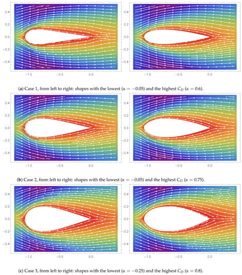
Figure 15. Streamline plots ($\mathrm{Re}=40$).

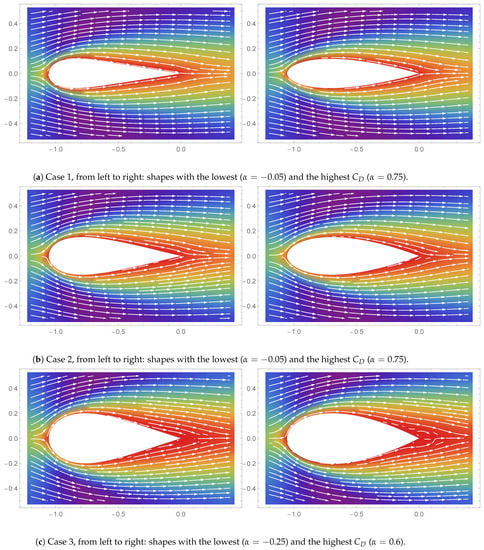
Figure 16. Streamline plots ($\mathrm{Re}=100$).

Figure 17 presents the curvature profiles of each LAC shape and its corresponding case with different colors. The darker blue curves represent the curvature profile $\kappa \left(\theta \right)$ of the LAC shapes with lower $\alpha$ values, where $\theta$ is the turning angle of the curve. As $\alpha$ increases, the color of the $\kappa \left(\theta \right)$ curve turns yellow. The purple-, red-, and orange-colored curves are the $\kappa \left(\theta \right)$ curves for the LAC shape with the highest $C_D$. Shapes with the lowest $C_D$ have an almost linear curvature $\kappa \left(\theta \right)$. However, $C_D$ also decreases as the $\kappa \left(\theta \right)$ of the LAC shape bends more.

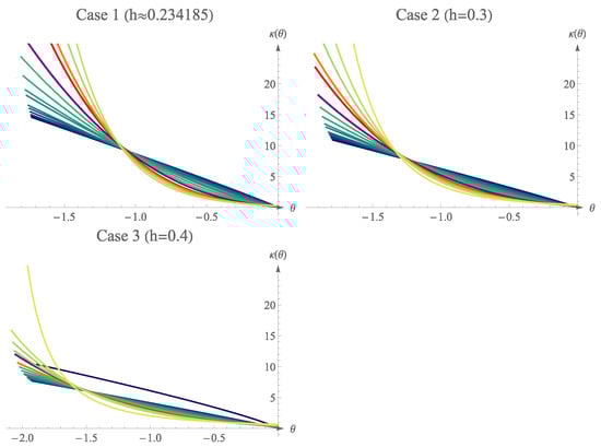
Figure 17. Curvature profiles of the objects.

Thus, it is clear that $C_D$ values for hydrofoils constructed with neutral (Nielsen’s Spiral $\alpha =0$) and divergent LACs ($\alpha <0$) are lower than those of convergent LACs ($\alpha >0$) and decrease as $\alpha$ decreases. The $C_D$ for hydrofoil constructed with convergent LACs ($\alpha >0$) does not increase or decrease monotonically as $\alpha$ increases or decreases. Instead, it gradually increases until it peaks at around $\alpha =0.6$ to $0.8$ and decreases as $\alpha$ increases.

Figure 18, Figure 19 and Figure 20 illustrates the distribution of time taken to reach steady state for each $\alpha$.

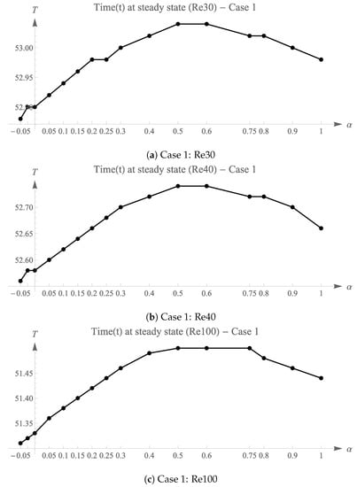
Figure 18. Final time (T) for each simulation with shapes of $h\approx 0.2$ (Case 1).

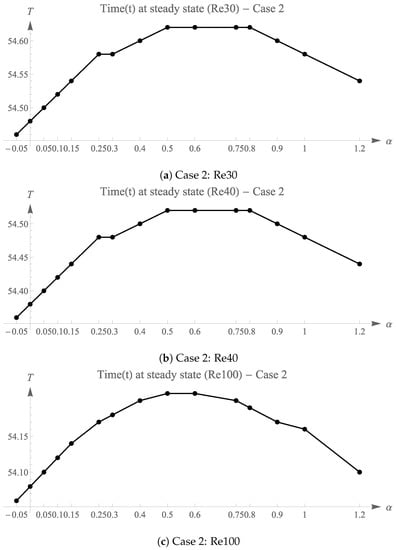
Figure 19. Final time (T) for each simulation with shapes of $h=0.3$ (Case 2).

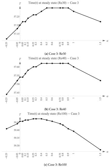
Figure 20. Final time (T) for each simulation with shapes of $h=0.4$ (Case 3).

6. Cluster Analysis of Drag Distribution

In this section, we clustered drag coefficients in Table 1, Table 2 and Table 3 using agglomerative hierarchical cluster analysis [29]. This step groups a similar drag distribution among the three different thicknesses of LAC hydrofoils with different Reynolds numbers. In this analysis, we employed the complete linkage approach [30], which merges two clusters with the closest maximum distance:

$$d_{\mathcal{AB}}=\underset{i\in \mathcal{A},j\in \mathcal{B}}{max}\left(d_{ij}\right)$$

(9)

where $d_{ij}$ is the distance and i and j are observations in clusters $\mathcal{A}$ and $\mathcal{B}$. The complete linkage method is coupled with the dissimilarity distance matrix obtained from Dynamic Time Warping (DTW) [31,32]. DTW is an algorithm that measures the similarity or distance between two arrays or time series of different lengths [32]. The difference between DTW and Euclidean distance is elucidated in Figure 21. Two data vectors were connected based on their minimal distance using DTW (green) and Euclidean (gray) distance [33]. The DTW method provides more accurate results than the Euclidean distance. DTW does not require the data sets to be equal in length and is not affected by shifting, unlike Euclidean distance. The detailed algorithm of DTW can be found in [32].

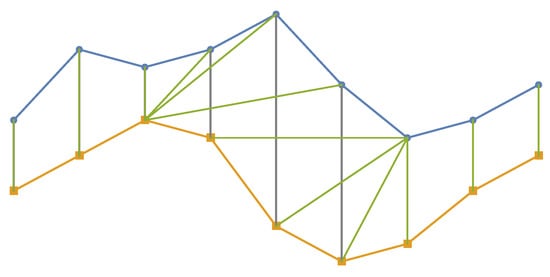
Figure 21. Visual comparison of matched points based on DTW (green) and Euclidean (gray) distance.

Since we have computed drag coefficients with different h values from different $\alpha$ values, the DTW algorithm matches it in a direction that minimizes the distance of drag coefficients between various $\alpha$ values without losing information. Figure 22 shows a dendrogram illustrating the clusters obtained. The x-axis is labeled based on the cases, and their corresponding Reynolds number, e.g., C1_30, represents Case 1 with LAC object thickness $h\approx 0.2$ and $\mathrm{Re}=30$.

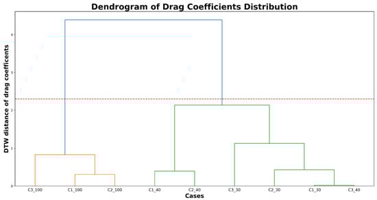
Figure 22. Dendrogram with two distinct clusters at a phenon line of distance 2.3.

The dendrogram has two distinct clusters at the phenon line of distance 2.1 onward with a Cophenetic correlation coefficient (CCC) value equal to 0.86. The CCC measuring close to 1 indicates that the accuracy of the resulting dendrogram preserves the pair-wise distances between the drag distributions. The first cluster in orange consists of Case 3 with $\mathrm{Re}=100$. We observed this cluster with the drag that may demonstrate the onset of unsteady flows at $\mathrm{Re}=100$ regardless of the LAC shapes. The second cluster (green) is the combination of cases with $\mathrm{Re}$ between 30 and 40, where the steady flow is guaranteed. Indeed, the two subclusters in green are also grouped based on the Reynolds number. The exception is C3_40, where the LAC hydrofoil has $h=0.4$ and $\mathrm{Re}=40$. The drag coefficients of C3_40 have a similar distribution to C1_30, where the LAC hydrofoil has $h\approx 0.2$ and $\mathrm{Re}=30$. Similarly, the case of C3_30 tends to move away from its own group of $\mathrm{Re}=30$. The formation of these two subclusters indicates that the distribution of drag coefficients does not rely on the Reynolds number alone; the thickness of the LAC objects also plays a pivotal role in the distribution of drag coefficients. This shows that the evaluation of Reynolds numbers based on chord length (or characteristic length) for streamlined-shape objects may somehow need to be reformulated and is still an open problem. This is true since the chord length of Case 3 hydrofoils, $c\approx 1$, started to become much closer to its thickness of 0.4. We recall that characteristic length directly influences the Reynolds numbers besides the mean velocity and the eddy viscosity. In other words, the “more accurate” Reynolds number for C3_30 can be very close to that of C1_40. Hence, they form a subcluster. The initial effort of cluster analysis can be helpful to study the resulting flow behavior (in this case, by only accessing their drag coefficients), even if the Reynolds numbers are not properly evaluated. Further studies need to be carried out to make the DTW algorithm more practical for flow characterizations, especially in the post-processing of CFD results.

7. Conclusions

Simulations of incompressible fluid flow around streamlined shapes built using LAC, with chord length $c\approx 1$ and thickness 0.234185, 0.3, and 0.4, were carried out. The results indicated that LAC shapes with negative $\alpha$ values, classified as divergent curves, and with almost linear curvature profiles $\kappa \left(\theta \right)$, representing Clothoids, generate the lowest drag. As $\alpha$ increases, the drag coefficient increases until it reaches a maximum of around $\alpha =0.6$ to 0.8 and then decreases. Flow separation was not observed for any of the three thickness variations except for the thickest LAC shape (Case 3, $h=0.4$) when $\mathrm{Re}=100$. The separation may have caused the difference in $C_D$ for Case 3 when $\mathrm{Re}=100$. It was also observed that the time used for the simulation to reach a steady state for Case 3 exhibits an entirely different trend compared to the other cases. Furthermore, the thickness of LAC objects can be varied to obtain similar drag coefficients for different Reynolds numbers. Thus, LAC with negative $\alpha$ values is better suited for designing submerged structures or objects that minimize drag.

The findings obtained in this study may help in decision-making in designing ship hulls or submerged bodies such as hydrofoils, underwater vehicles and structures, and marine-bio-logging tags [34]. A designer may now opt to prioritize LAC with negative values in designing such objects to minimize drag. They can also anticipate how the drag coefficient varies as the shape of the LAC changes. This shall act as a step towards implementing LACs in submerged objects or ship-hull designs. Additionally, this paper presents a new algorithm for generating the LAC shapes required to construct a LAC hydrofoil. The resulting LAC satisfies the user-specified height, length, $G^1$ Hermite data at one end, and $G^0$ Hermite data at the other.

For future research, we wish to extend our study to incompressible turbulent flow situations. We also hope to simulate incompressible flows around three-dimensional objects built with LAC or LA surfaces and examine their hydrodynamics and vector-field topology using an emerging method called Topological Data Analysis [35].

References

- Yoshimoto, F.; Harada, T. Analysis of the characteristics of curves in natural and factory products. In Proceedings of the 2nd IASTED International Conference on Vizualization, Imaging and Image Processing, Malaga, Spain, 9–12 September 2002; pp. 276–281. [Google Scholar]
- Harada, T.; Yoshimoto, F.; Moriyama, M. Aesthetic curve in the field of industrial design. In Proceedings of the IEEE Symposium on Visual Languages, Tokyo, Japan, 13–16 September 1999; pp. 38–47. [Google Scholar] [CrossRef]
- Miura, K.T. A general equation of aesthetic curves and its self-affinity. Comput.-Aided Des. Appl. 2006, 3, 457–464. [Google Scholar] [CrossRef]
- Gobithaasan, R.U.; Miura, K.T. Logarithmic curvature graph as a shape interrogation tool. Appl. Math. Sci. 2014, 8, 755–765. [Google Scholar] [CrossRef]
- Miura, K.T.; Shibuya, D.; Gobithaasan, R.U.; Usuki, S. Designing log-aesthetic splines with G2 continuity. Comput.-Aided Des. Appl. 2013, 10, 1021–1032. [Google Scholar] [CrossRef]
- Arslan, A.; Tari, E.; Ziatdinov, R.; Nabiyev, R.I. Transition curve modeling with kinematical properties: Research on Log-aesthetic curves. CAD Solut. LLC 2014, 11, 509–517. [Google Scholar] [CrossRef][Green Version]
- Gobithaasan, R.U.; Yip, S.W.; Miura, K.T.; Madhavan, S. Optimal path smoothing with Log-aesthetic curves based on shortest distance, minimum bending energy or curvature variation energy. Comput.-Aided Des. Appl. 2020, 17, 639–658. [Google Scholar] [CrossRef]
- Kineri, Y.; Endo, S.; Maekawa, T. Surface design based on direct curvature editing. CAD Comput. Aided Des. 2014, 55, 1–12. [Google Scholar] [CrossRef]
- Suzuki, T. Application of Log-aesthetic curves to the eaves of a wooden house. In Proceedings of the 4th International Conference on Archi-Cultural Interactions through the Silk Road, Nishinomiya, Japan, 16–18 July 2016; pp. 67–70. [Google Scholar]
- Levien, R.; Séquin, C.H. Interpolating Splines: Which is the fairest of them all? Comput.-Aided Des. Appl. 2009, 6, 91–102. [Google Scholar] [CrossRef]
- Imai, T.; Shibutani, T.; Matsui, K.; Kumagai, S.; Tran, D.T.; Mu, K.; Maekawa, T. Curvature sensitive analysis of axially compressed cylindrical tubes with corrugated surface using isogeometric analysis and experiment. Comput. Aided Geom. Des. 2016, 49, 17–30. [Google Scholar] [CrossRef]
- John, V. Reference values for drag and lift of a two-dimensional time-dependent flow around a cylinder. Int. J. Numer. Methods Fluids 2004, 44, 777–788. [Google Scholar] [CrossRef]
- Loy, K.C.; Bourgault, Y. On efficient high-order semi-implicit time-stepping schemes for unsteady incompressible Navier–Stokes equations. Comput. Fluids 2017, 148, 166–184. [Google Scholar] [CrossRef]
- Wo, M.S.; Gobithaasan, R.U.; Miura, K.T.; Loy, K.C.; Yasmeen, S.; Harun, F.N. Log-aesthetic curves and their relation to fluid flow patterns in terms of streamlines. J. Comput. Des. Eng. 2020, 8, 55–68. [Google Scholar] [CrossRef]
- Quartapelle, L. Numerical Solution of the Incompressible Navier–Stokes Equations; Springer Science & Business Media: Berlin, Germany, 1993. [Google Scholar] [CrossRef]
- Girault, V.; Raviart, P.A. Mathematical Foundation of the Stokes Problem BT—Finite Element Methods for Navier–Stokes Equations: Theory and Algorithms; Springer: Berlin/Heidelberg, Germany, 1986; pp. 1–111. [Google Scholar] [CrossRef]
- Babuška, I. The finite element method with Lagrangian multipliers. Numer. Math. 1973, 20, 179–192. [Google Scholar] [CrossRef]
- Girault, V.; Raviart, P.A. Numerical Solution of the Stokes Problem in the Primitive Variables BT—Finite Element Methods for Navier–Stokes Equations: Theory and Algorithms; Springer: Berlin/Heidelberg, Germany, 1986; pp. 112–192. [Google Scholar] [CrossRef]
- Barrenechea, G.R.; Wachtel, A. The inf-sup stability of the lowest order Taylor–Hood pair on affine anisotropic meshes. IMA J. Numer. Anal. 2020, 40, 2377–2398. [Google Scholar] [CrossRef]
- Temam, R. Navier–Stokes Equations: Theory and Numerical Analysis; American Mathematical Society: Chelsea, MA, USA, 2000. [Google Scholar]
- Yoshida, N.; Saito, T. Interactive aesthetic curve segments. Vis. Comput. 2006, 22, 896–905. [Google Scholar] [CrossRef]
- Kanaya, I.; Nakano, Y.; Sato, K. Classification of Aesthetic Curves and Surfaces for Industrial Designs. Des. Discourse 2007, 2, 4. [Google Scholar]
- Gobithasan, R.; Ali, J. Towards G2 curve design with Timmer parametric cubic. In Proceedings of the Proceedings. International Conference on Computer Graphics, Imaging and Visualization, Penang, Malaysia, 2 July 2004; pp. 109–114. [Google Scholar] [CrossRef]
- Hardie, S. Drag Estimations on Experimental Aircraft Using CFD; Technical Report; Mälardalens Högskola: Västerås, Sweden, 2006. [Google Scholar]
- Khchine, Y.E.; Sriti, M. Boundary layer and amplified grid effects on aerodynamic performances of S809 airfoil for horizontal axis wind turbine (HAWT). J. Eng. Sci. Technol. 2017, 12, 3011–3022. [Google Scholar]
- Hecht, F. New development in freefem+. J. Numer. Math. 2012, 20, 251–265. [Google Scholar] [CrossRef]
- Anderson, J.D. Fundamentals of Aerodynamics, 6th ed.; McGraw-Hill Higher Education: New York, NY, USA, 2017. [Google Scholar]
- Anderson, J.D. Introduction to Flight, 5th ed.; McGraw-Hill Higher Education: New York, NY, USA, 2004. [Google Scholar]
- Everitt, B.S.; Landau, S.; Leese, M.; Stahl, D. Cluster Analysis, 5th ed.; John Wiley & Sons: Hoboken, NJ, USA, 2011. [Google Scholar]
- Everitt, B.S.; Dunn, G. Applied Multivariate Data Analysis, 2nd ed.; John Wiley & Sons: Hoboken, NJ, USA, 2001. [Google Scholar] [CrossRef]
- Aghabozorgi, S.; Seyed Shirkhorshidi, A.; Teh, Y.W. Time-series clustering—A decade review. Inf. Syst. 2015, 53, 16–38. [Google Scholar] [CrossRef]
- Senin, P. Dynamic Time Warping Algorithm Review. Science 2008, 855, 40. [Google Scholar]
- Sobolewska, E. Dynamic Time Warping (DTW) as a Mean to Cluster Time Series. 2022. Available online: https://rstudio-pubs-static.s3.amazonaws.com/474160_0761428e8683401e941a92a4177254a4.html (accessed on 1 December 2022).
- Fiore, G.; Anderson, E.; Garborg, C.S.; Murray, M.; Johnson, M.; Moore, M.J.; Howle, L.; Shorter, K.A. From the track to the ocean: Using flow control to improve marine bio-logging tags for cetaceans. PLoS ONE 2017, 12, e0170962. [Google Scholar] [CrossRef] [PubMed]
- Bridel-Bertomeu, T.; Fovet, B.; Tierny, J.; Vivodtzev, F. Topological Analysis of High Velocity Turbulent Flow. In Proceedings of the 2019 IEEE 9th Symposium on Large Data Analysis and Visualization (LDAV), Vancouver, BC, Canada, 21 October 2019; pp. 87–88. [Google Scholar] [CrossRef]
Disclaimer/Publisher’s Note: The statements, opinions and data contained in all publications are solely those of the individual author(s) and contributor(s) and not of MDPI and/or the editor(s). MDPI and/or the editor(s) disclaim responsibility for any injury to people or property resulting from any ideas, methods, instructions or products referred to in the content. |
© 2022 by the authors. Licensee MDPI, Basel, Switzerland. This article is an open access article distributed under the terms and conditions of the Creative Commons Attribution (CC BY) license (https://creativecommons.org/licenses/by/4.0/).