Dynamical Analysis of Nutrient-Phytoplankton-Zooplankton Model with Viral Disease in Phytoplankton Species under Atangana-Baleanu-Caputo Derivative

Abstract

A mathematical model of the nutrient-phytoplankton-zooplankton associated with viral infection in phytoplankton under the Atangana-Baleanu derivative in Caputo sense is investigated in this study. We prove the theoretical results for the existence and uniqueness of the solutions by using Banach’s and Sadovskii’s fixed point theorems. The notion of various Ulam’s stability is used to guarantee the context of the stability analysis. Furthermore, the equilibrium points and the basic reproduction numbers for the proposed model are provided. The Adams type predictor-corrector algorithm has been applied for the theoretical confirmation to establish the approximate solutions. A variety of numerical plots corresponding to various fractional orders between zero and one are presented to describe the dynamical behavior of the fractional model under consideration.

1. Introduction

In nature, the basis of all aquatic food chains is plankton, which can be categorized into dual types, namely, phytoplankton and zooplankton [1,2]. Plankton that transforms mineral nutrients into ancient biotic material handling exterior energy from the sun is called phytoplankton, whereas plankton that needs to survive by eating phytoplankton or small aquatic animals is called zooplankton [3]. The succession and society of phytoplankton could impact the environmental circumstances of the ecosystem. On the one hand, plankton species have positive effects on the environment, such as giving food to sea life, oxygenation, controlling and improving the quality of the water and circulating the nutrients, especially nitrogen and phosphorus, that are natural sections of aquatic ecosystems and encourage the growth of algae and aquatic plants [4,5]. On the other hand, plankton has harmful effects, such as economic losses to fisheries and tourism due to plankton blooms that happen when the number of phytoplankton species increases very fast until they cover the surface of the ocean or river. This means that they block sunlight from reaching other organisms. This phenomenon affects the depletion of oxygen levels in the water and can ultimately lead to aquatic plant and fish die-offs [6,7,8,9,10,11]. Furthermore, nutritional availability, as a result of the enhanced nutrient response to the increasing phytoplankton population, is one of the major variables impacting phytoplankton concentration. Another factor is viruses in natural aquatic ecosystems, which have a significant impact on the phytoplankton population.

Real-world mathematical modeling is an effective method for forecasting some of their ecological and biological components. The model’s validity determines the applicability of this mathematical approximation. There are many researchers who are interested in the interaction between phytoplankton, zooplankton, nutrients, and viruses. The dynamic interaction between them has fascinated scientific and mathematical ecology’s curiosity. A variety of mathematical models, which consist of differential equations, are constructed to study the dynamics. In 2002, The dynamics of nutrient-driven phytoplankton blooms were reported by Huppert et al. [12], who utilized the initial conditions to predict how the peak of the bloom would be determined. In 2004, the phytoplankton-zooplankton system was modeled as a predator-prey system by Singh et al. [13]. The dynamical behavior of their system was studied both analytically and numerically in terms of stability and persistence. In 2007, Chakraborty et al. [14] investigated a mathematical model of nutrient-phytoplankton to better understand the dynamics of repeating bloom occurrences in the attendance of harmful toxins emitted by toxin-building phytoplankton. Recently, in 2019, Nath et al. [15] analyzed the stability of different stationary points for the system of nutrient–phytoplankton–zooplankton ($\mathbb{NPZ}$) with the viral disease of phytoplankton individuals. In a later year, Nath et al. [16] extended their work to construct and analyze a mathematical model for plankton dynamics in $\mathbb{NPZ}$ model affected by a viral infection in the population of phytoplankton. They verified the basic reproduction number and also obtained the sufficient condition of Hopf-Bifurcation of the model. See [17,18,19,20] for a list of further works and references.

Alternatively, as we know, the mathematical models ignore the memory effect since they are only integer order derivatives, whereas the concept of differentiation with a non-local operator also known as fractional differentiation has been recognized as a very powerful mathematical instrument able to understand memory and hereditary features in most biological systems. In addition, The response of the system is determined not only by its current state but also by its entire history. Therefore, the ordinary integer-order derivative does not cover this memory effect because it is a local operator. Concurrently, fractional calculus has been widely interested by many researchers. It is an arbitrary order generalized differential and integral operator. Various definitions of fractional derivative and integral operators like Caputo–Liouville ($\mathbb{CL}$), Caputo–Katugumpola ($\mathbb{CK}$), Caputo–Fabrizio ($\mathbb{CF}$), Atangana–Baleanu–Riemann ($\mathbb{ABR}$), Atangana–Baleanu–Caputo ($\mathbb{ABC}$), and so on. They have been defined and used in conjunction with differential systems in many works of literature, including the $\mathbb{NPZ}$ problems. For example, in 2018, Ghanbar et al. [21] studied the model of $\mathbb{NPZ}$ with variable order fractional differential operators of $\mathbb{CL}$, $\mathbb{CF}$, and Atangana-Baleanu ($\mathbb{AB}$). The dynamical effect of the interaction between nutrients and phytoplankton with zooplankton was described in their work. In 2020, Shi et al. [22] used the fractional-order stability theory to investigate the existence, stability of equilibrium points, and Hopf bifurcation for an arbitrary order mathematical model with the $\mathbb{CL}$ operator under the delay of nutrient–phytoplankton–toxic phytoplankton–zooplankton, Furthermore, we offer the reader to explore the interesting other problems using the fractional derivative as in 2020, Thabet et al. [23] studied and analyzed the fractional model under $\mathbb{ABC}$ derivative of a novel Coronavirus disease (COVID-19). In the same year, Kumar et al. [24], used the fractional derivative which contains the Mittag–Leffler type of kernel to present an analysis of the fractional model of the Klein–Gordon ($\mathbb{K}$-$\mathbb{G}$) equation. In 2021, Rahman et al. [25] studied the $\mathbb{ABC}$ derivative of the fractional model for drinking behavior. They proved the existence and uniqueness of the solution and illustrated the numerical simulation of the model, see more works [26,27,28,29,30] and references cited therein.

Motivated by the previous description to the best of our knowledge, the main aim of this research is to develop a mathematical model governed by fractional-order differential equations for investigating the impact of memory on the $\mathbb{NPZ}$ model. Moreover, the mathematical model of $\mathbb{NPZ}$ on $\mathbb{ABC}$–fractional derivative operator has not been discussed. Therefore, in this paper, the $\mathbb{ABC}$–fractional derivative operator will be applied to the $\mathbb{NPZ}$ model proposed by [16], which is the paper’s originality and ingenuity (the $\mathbb{ABC}$-$\mathbb{FNPZ}$ model). Furthermore, we are interested in covering this margin by taking this model under the $\mathbb{ABC}$–fractional derivative with order $\alpha$.

The paper is organized as follows: fundamental knowledge of $\mathbb{ABC}$-fractional operators and definitions of fixed point theorems are provided in part 2. Part 3 is devoted to proving the uniqueness of solutions for the $\mathbb{ABC}$-$\mathbb{FNPZ}$ model (3) via fixed point theory of Banach’s type, while the existence result forthe $\mathbb{ABC}$-$\mathbb{FNPZ}$ model (3) are investigated via Sodovskii’s fixed point theorem. The Ulam-Hyers stability and Ulam-Hyers-Rassias stability of the $\mathbb{ABC}$-$\mathbb{FNPZ}$ model (3) are extensively obtained in part 4. Further, simulation results are demonstrated to confirm the theoretical results. The discussions of the $\mathbb{ABC}$-$\mathbb{FNPZ}$ model are studied in part 5 to offer better learning of the obtained results. Finally, part 6 concludes by explaining the conclusions and italicizing the results obtained in this paper.

2. Mathematical Backgrounds

Before moving on to model formulation, it is important to review several key definitions related to the Atangana-Baleanu fractional operators [31].

2.1. Basic Definitions

Definition 1

([31]). Assume that $g\in {\mathcal{H}}^1(a,b)$ is a function with $a<b$. Then the $\mathbb{ABC}$-fractional derivative of g of order $\alpha \in [0,1]$ is given by

$${}_t^{\mathbb{ABC}}{\mathfrak{D}}_a^{\alpha }g\left(t\right)=\left\{\begin{array}{c}{\displaystyle \frac{\mathbb{AB}\left(\alpha \right)}{1-\alpha }{\int }_a^t{\mathbb{E}}_{\alpha }\left[-\frac{\alpha }{1-\alpha }{(t-s)}^{\alpha }\right]g^{\prime }\left(s\right)ds,0<\alpha <1,}\hfill \\ {\displaystyle \frac{dg\left(t\right)}{dt},\alpha =1,}\hfill \end{array}\right.$$

(1)

where $\mathbb{AB}\left(\alpha \right)=1-\alpha +\alpha /\mathsf{\Gamma }\left(\alpha \right)$ with $\mathbb{AB}\left(0\right)=\mathbb{AB}\left(1\right)=1$, and

$${\mathbb{E}}_{\alpha }\left(u\right)=\sum _{n=0}^{\infty }\frac{u^n}{\mathsf{\Gamma }(\alpha n+1)},u,\alpha \in \mathbb{C},Re\left(\alpha \right)>0.$$

Remark 1.

Definition 1 will be productive for investigating real-world problems, and it would also have great dominance when applying the Laplace transform to solve various physical problems with initial conditions. However, when $\alpha =0$ we do not recover the initial function except when at the origin the function disappears.

To escape previous problem, we present the following definition:

Definition 2

([31]). Assume that $g\in {\mathcal{H}}^1(a,b)$ is a function with $a<b$. Then the $\mathbb{ABR}$-fractional derivative of g of order $\alpha \in [0,1]$ is given by

$${}_t^{\mathbb{ABR}}{\mathfrak{D}}_a^{\alpha }g\left(t\right)=\frac{\mathbb{AB}\left(\alpha \right)}{1-\alpha }\frac{d}{dt}{\int }_a^t{\mathbb{E}}_{\alpha }\left[-\frac{\alpha }{1-\alpha }{(t-s)}^{\alpha }\right]g\left(s\right)ds.$$

(2)

Remark 2.

Definitions 1 and 2 have a non-local kernal. Furthermore, in Definition 1 when the function is the constant we obtain zero.

Definition 3

([31]). The $\mathbb{ABC}$-fractional integral of a function $g\in {\mathcal{C}}^1(a,b)$ is given by

$${}_t^{\mathbb{AB}}{\mathcal{I}}_a^{\alpha }g\left(t\right)=\frac{1-\alpha }{\mathbb{AB}\left(\alpha \right)}g\left(t\right)+\frac{\alpha }{\mathbb{AB}\left(\alpha \right)\mathsf{\Gamma }\left(\alpha \right)}{\int }_a^t{\left(t-s\right)}^{\alpha -1}g\left(s\right)ds.$$

Remark 3.

In Definition 3, when we take $\alpha =0$ we recover the initial function, and if $\alpha =1$, we get the classical integral operator.

Lemma 1

([31]). The relation between the $\mathbb{ABC}$-fractional derivative and the $\mathbb{AB}$-fractional integral of a function $g\in {\mathcal{H}}^1(a,b)$ is

$${}_t^{\mathbb{AB}}{\mathcal{I}}_a^{\alpha }\left({}_t^{\mathbb{ABC}}{\mathfrak{D}}_a^{\alpha }g\left(t\right)\right)=g\left(t\right)-g\left(a\right).$$

2.2. Some Fixed Point Theorems

Definition 4

([32]). Assume that $\mathcal{E}$ is a Banach space. Hence the operator $\mathcal{K}:\mathcal{E}\to \mathcal{E}$ is a contraction if

$$\parallel \mathcal{K}u-\mathcal{K}v\parallel \le \mathcal{L}\parallel u-v\parallel ,\forall u,v,\in \mathcal{E},\mathcal{L}\in (0,1).$$

Lemma 2

([32]). Assume that $\mathcal{B}$ is a non-empty closed subset of $\mathcal{E}$ where $\mathcal{E}$ is a Banach space. Hence any contraction mapping $\mathcal{K}$ from $\mathcal{B}$ into itself has a unique fixed point.

Definition 5

([32]). Assume that $\mathcal{E}$ is a Banach space and $\mathcal{K}:\mathcal{E}\to \mathcal{E}$ is a mapping. $\mathcal{K}$ is called a nonlinear contraction if there is a continuous non-decreasing function $\mathsf{\Phi }:{\mathbb{R}}^{+}\to {\mathbb{R}}^{+}$ such that $\mathsf{\Phi }\left(0\right)=0$ and $\mathsf{\Phi }\left(ϵ\right)<ϵ$, for any $ϵ>0$ with

$$\parallel \mathcal{K}u-\mathcal{K}vs.\parallel \le \mathsf{\Phi }(\parallel u-vs.\parallel ),\forall u,vs.\in \mathcal{E}.$$

Definition 6

([33]). Consider a bounded subset $\mathcal{B}$ of $(X,d)$. The Kuratowski measure of non-compactness, $\alpha \left(\mathcal{B}\right)$, is given by

$$\alpha \left(\mathcal{B}\right):=inf\left\{ϵ>0:thereexitsfinitelymanysets{\mathcal{B}}_{i}suchthat\mathcal{B}=\bigcup _{i=1}^n{\mathcal{B}}_i\mathrm{and}M\left({\mathcal{B}}_i\right)\le ϵ\right\},$$

where $M\left({\mathcal{B}}_i\right)=sup\left\{\left|u-\overline{u}\right|:u,\overline{u}\in {\mathcal{B}}_i\right\}$.

Definition 7

([33]). Consider a bounded and continuous function $\mathcal{K}:Dom\left(\mathcal{K}\right)\subseteq \mathcal{B}\to \mathcal{B}$ on $\mathcal{B}$. For an arbitrary bounded set $\mathcal{D}\subset Dom\left(\mathcal{K}\right)$, the map $\mathcal{K}$ is condensing if $\alpha \left(\mathcal{K}\right(\mathcal{D}\left)\right)<\alpha \left(\mathcal{K}\right)$, in which α is defined previous part.

Lemma 3

([34]). Assume that ${\mathcal{K}}_1$, ${\mathcal{K}}_2:\mathcal{B}\subseteq \mathcal{E}\to \mathcal{E}$. The operator ${\mathcal{K}}_1+{\mathcal{K}}_2$ is condensing if satisfies the following assumptions $\left(i\right)$${\mathcal{K}}_1$ is $\mathcal{L}$-contraction; that is, for any u, $v\in \mathcal{B}$ and there exists $\mathcal{L}\in (0,1)$, such that $\parallel {\mathcal{K}}_{1}x-{\mathcal{K}}_{1}vs.\parallel \le \mathcal{L}\parallel u-vs.\parallel$; $\left(ii\right)$${\mathcal{K}}_2$ is compact.

Lemma 4

([35]). Consider the bounded, closed and convex subset $\mathcal{D}$ of $\mathcal{E}$ and the condensing mapping $\mathcal{K}:\mathcal{D}\to \mathcal{D}$. Then $\mathcal{K}$ has a fixed point.

2.3. Model Construction

As stated afore, this paper is based on the proposed model [16], where the populations are separated into four groups representing concentration status. They are the concentration of the nutrient at time t presented by nutrient group; $\mathcal{N}\left(t\right)$, the concentration of susceptible phytoplankton at time t presented by susceptible group; $\mathcal{S}\left(t\right)$, the concentration of infected phytoplankton at time t presented by infected group; $\mathcal{I}\left(t\right)$, and the concentration of zooplankton at time t presented by zooplankton group; $\mathcal{Z}\left(t\right)$. Initially, for the model under consideration, we insert the integer order of the ordinary $\mathbb{NPZ}$ model with the non-integer order (fractional-order $\alpha$). It will be expanded to the fractional system by taking the ordinary derivative $d/dt$ to fractional derivative in the context of $\mathbb{ABC}$–derivative ${{}_t^{\mathbb{ABC}}\mathfrak{D}}_0^{\alpha }$. The rebuilt $\mathbb{NPZ}$ model under viral infection in phytoplankton species under the $\mathbb{ABC}$–fractional derivative is recommended as:

$$\left\{\begin{array}{c}{\displaystyle {{}_t^{\mathbb{ABC}}\mathfrak{D}}_0^{\alpha }\mathcal{N}\left(t\right)={\xi }^{\alpha }(N_0^{\alpha }-\mathcal{N})-a^{\alpha }\mathcal{S}u\left(\mathcal{N}\right)-b^{\alpha }\mathcal{I}v\left(\mathcal{N}\right)-c^{\alpha }\mathcal{Z}w\left(\mathcal{N}\right),}\hfill \\ {\displaystyle {{}_t^{\mathbb{ABC}}\mathfrak{D}}_0^{\alpha }\mathcal{S}\left(t\right)=a^{\alpha }\mathcal{S}u\left(\mathcal{N}\right)-{\beta }^{\alpha }\mathcal{S}\mathcal{I}-m^{\alpha }\mathcal{Z}g\left(\mathcal{S}\right)-{\eta }_1^{\alpha }\mathcal{S},}\hfill \\ {\displaystyle {{}_t^{\mathbb{ABC}}\mathfrak{D}}_0^{\alpha }\mathcal{I}\left(t\right)=b^{\alpha }\mathcal{I}v\left(\mathcal{N}\right)+{\beta }^{\alpha }\mathcal{S}\mathcal{I}-n^{\alpha }\mathcal{Z}g\left(\mathcal{I}\right)-{\eta }_2^{\alpha }\mathcal{I},}\hfill \\ {\displaystyle {{}_t^{\mathbb{ABC}}\mathfrak{D}}_0^{\alpha }\mathcal{Z}\left(t\right)=c^{\alpha }\mathcal{Z}w\left(\mathcal{N}\right)+e_1^{\alpha }{m}^{\alpha }\mathcal{Z}g\left(\mathcal{S}\right)+e_2^{\alpha }{n}^{\alpha }\mathcal{Z}g\left(\mathcal{I}\right)-{\eta }_3^{\alpha }\mathcal{Z},}\hfill \end{array}\right.$$

(3)

with the initial condition $(\mathcal{N},\mathcal{S},\mathcal{I},\mathcal{Z})=({\mathcal{N}}_0,{\mathcal{S}}_0,{\mathcal{I}}_0,{\mathcal{Z}}_0)$ where ${\mathcal{N}}_0$, ${\mathcal{S}}_0$, ${\mathcal{I}}_0$, ${\mathcal{Z}}_0>0$. Here, the functions $u\left(\mathcal{N}\right)$, $v\left(\mathcal{N}\right)$, and $w\left(\mathcal{N}\right)$ represent the nutrient uptake rates of susceptible phytoplankton, infected phytoplankton and, zooplankton, respectively. The functions $u\left(\mathcal{N}\right)$, $v\left(\mathcal{N}\right)$, and $w\left(\mathcal{N}\right)$ satisfy the following assumptions:

(i)

The functions $u\left(\mathcal{N}\right)$ and $v\left(\mathcal{N}\right)$ are continuous defined on $[0,\infty )$;

(ii)

The functions $u\left(0\right)=v\left(0\right)=0$, $du/d\mathcal{N}>0$, $dv/d\mathcal{N}>0$, and ${lim}_{t\to \infty }u\left(\mathcal{N}\right)={lim}_{t\to \infty }v\left(\mathcal{N}\right)=1$;

(iii)

The function $g\left(x\right)$ is the response function representing herbivore grazing where g is continuous on $[0,\infty )$ and satisfies $g\left(0\right)=0$, $g^{\prime }\left(x\right)>0$, and $\underset{t\to \infty }{lim}g\left(u\right)=1$, $u=\{\mathcal{S},\mathcal{I}\}$.

The descriptions of all non-negative parameters are listed in Table 1.

Table 1. The details of parameters of the $\mathbb{NPZ}$ model (3).

Parameter	Details of the Parameter
$N_0$	The constant input of nutrient concentration;
$\xi$	The washout rate of the nutrient;
${\eta }_1$	The mortality rate of susceptible phytoplankton group;
${\eta }_2$	The mortality rate of infected phytoplankton group;
${\eta }_3$	The mortality rate of zooplankton group;
a	The maximal intake nutrient rate for susceptible phytoplankton species;
b	The maximal intake nutrient rate for infected phytoplankton species;
c	The maximal intake nutrient rate for zooplankton species;
$\beta$	The force of infection between the both phytoplankton groups;
m	The predation rate of zooplankton for susceptible phytoplankton;
n	The predation rate of zooplankton for infected phytoplankton;
$e_1$	The conversion efficiency due to consumption of susceptible
	phytoplankton;
$e_2$	The conversion efficiency due to consumption of infected phytoplankton;

2.4. The Equilibrium Points of the $\mathbb{ABC}$-$\mathbb{FNPZ}$ Model (3)

Next, we show the equilibrium points and verify the stability of their associated equilibria with the help of the basic reproduction numbers.

Investigating the equilibrium points of the dynamics models helps to better understand the dynamic complexity of the models. To reach the equilibrium points for the $\mathbb{ABC}$-$\mathbb{FNPZ}$ model (3), we take

$${{}_t^{\mathbb{ABC}}\mathfrak{D}}_0^{\alpha }\mathcal{N}\left(t\right)=0,{{}_t^{\mathbb{ABC}}\mathfrak{D}}_0^{\alpha }\mathcal{S}\left(t\right)=0,{{}_t^{\mathbb{ABC}}\mathfrak{D}}_0^{\alpha }\mathcal{I}\left(t\right)=0,{{}_t^{\mathbb{ABC}}\mathfrak{D}}_0^{\alpha }\mathcal{Z}\left(t\right)=0.$$

Then, the eight equilibrium points are analyzed as follows:

$$\begin{array}{ccc}\hfill {\mathfrak{E}}_0^{*}& =& ({\mathcal{N}}_0^{*},0,0,0),{\mathfrak{E}}_1^{*}=({\mathcal{N}}_1^{*},{\mathcal{S}}_1^{*},0,0),{\mathfrak{E}}_2^{*}=({\mathcal{N}}_2^{*},0,{\mathcal{I}}_2^{*},0),\hfill \\ \hfill {\mathfrak{E}}_3^{*}& =& ({\mathcal{N}}_3^{*},0,0,{\mathcal{Z}}_3^{*}),{\mathfrak{E}}_4^{*}=({\mathcal{N}}_4^{*},0,{\mathcal{I}}_4^{*},{\mathcal{Z}}_4^{*}),{\mathfrak{E}}_5^{*}=({\mathcal{N}}_5^{*},{\mathcal{S}}_5^{*},0,{\mathcal{Z}}_5^{*}),\hfill \\ \hfill {\mathfrak{E}}_6^{*}& =& ({\mathcal{N}}_6^{*},{\mathcal{S}}_6^{*},{\mathcal{I}}_6^{*},0),{\mathfrak{E}}_7^{*}=({\mathcal{N}}_7^{*},{\mathcal{S}}_7^{*},{\mathcal{I}}_7^{*},{\mathcal{Z}}_7^{*}),\hfill \end{array}$$

where ${\mathcal{N}}_0^{*}=N_0^{\alpha }$,

$$\begin{array}{ccc}\hfill {\mathcal{N}}_1^{*}& =& u^{-1}\left(\frac{{\eta }_1^{\alpha }}{a^{\alpha }}\right),{\mathcal{S}}_1^{*}=\frac{{\xi }^{\alpha }}{{\eta }_1^{\alpha }}\left[N_0^{\alpha }-u^{-1}\left(\frac{{\eta }_1^{\alpha }}{a^{\alpha }}\right)\right],\hfill \\ \hfill {\mathcal{N}}_2^{*}& =& v^{-1}\left(\frac{{\eta }_2^{\alpha }}{b^{\alpha }}\right),{\mathcal{I}}_2^{*}=\frac{{\xi }^{\alpha }}{{\eta }_2^{\alpha }}\left[N_0^{\alpha }-v^{-1}\left(\frac{{\eta }_2^{\alpha }}{b^{\alpha }}\right)\right],\hfill \\ \hfill {\mathcal{N}}_3^{*}& =& w^{-1}\left(\frac{{\eta }_3^{\alpha }}{c^{\alpha }}\right),{\mathcal{Z}}_3^{*}=\frac{{\xi }^{\alpha }}{{\eta }_3^{\alpha }}\left[N_0^{\alpha }-w^{-1}\left(\frac{{\eta }_3^{\alpha }}{c^{\alpha }}\right)\right],\hfill \\ \hfill {\mathcal{I}}_4^{*}& =& g^{-1}\left(\frac{{\eta }_3^{\alpha }-c^{\alpha }w\left({\mathcal{N}}_4^{*}\right)}{e_2^{\alpha }{n}^{\alpha }}\right),{\mathcal{Z}}_4^{*}=\frac{1}{{\eta }_3^{\alpha }-c^{\alpha }w\left({\mathcal{N}}_4^{*}\right)}\left[e_2^{\alpha }(b^{\alpha }v\left({\mathcal{N}}_4^{*}\right)-{\eta }_2^{\alpha }){\mathcal{I}}_4^{*}\right],\hfill \\ \hfill {\mathcal{S}}_5^{*}& =& g^{-1}\left(\frac{{\eta }_3^{\alpha }-c^{\alpha }w\left({\mathcal{N}}_5^{*}\right)}{e_1^{\alpha }{m}^{\alpha }}\right),{\mathcal{Z}}_5^{*}=\frac{1}{{\eta }_3^{\alpha }-c^{\alpha }w\left({\mathcal{N}}_5^{*}\right)}\left[e_1^{\alpha }(a^{\alpha }u\left({\mathcal{N}}_5^{*}\right)-{\eta }_1^{\alpha }){\mathcal{S}}_5^{*}\right],\hfill \\ \hfill {\mathcal{S}}_6^{*}& =& \frac{{\eta }_2^{\alpha }-b^{\alpha }v\left({\mathcal{N}}_6^{*}\right)}{{\beta }^{\alpha }},{\mathcal{I}}_6^{*}=\frac{a^{\alpha }u\left({\mathcal{N}}_6^{*}\right)-{\eta }_1^{\alpha }}{{\beta }^{\alpha }},\hfill \end{array}$$

${\mathcal{N}}_4^{*}$ is the positive solution of

$${\xi }^{\alpha }(N_0^{\alpha }-{\mathcal{N}}_4^{*})({\eta }_3^{\alpha }-c^{\alpha }w\left({\mathcal{N}}_4^{*}\right))-[b^{\alpha }v\left({\mathcal{N}}_4^{*}\right)({\eta }_3^{\alpha }-c^{\alpha }w\left({\mathcal{N}}_4^{*}\right))+c^{\alpha }w\left({\mathcal{N}}_4^{*}\right)e_2^{\alpha }(b^{\alpha }v\left({\mathcal{N}}_4^{*}\right)-{\eta }_2^{\alpha })]{\mathcal{I}}_4^{*}=0,$$

${\mathcal{N}}_5^{*}$ is the positive solution of

$${\xi }^{\alpha }(N_0^{\alpha }-{\mathcal{N}}_5^{*})({\eta }_3^{\alpha }-c^{\alpha }w\left({\mathcal{N}}_5^{*}\right))-[a^{\alpha }u\left({\mathcal{N}}_5^{*}\right)({\eta }_3^{\alpha }-c^{\alpha }w\left({\mathcal{N}}_5^{*}\right))+c^{\alpha }w\left({\mathcal{N}}_5^{*}\right)e_1^{\alpha }(a^{\alpha }u\left({\mathcal{N}}_5^{*}\right)-{\eta }_1^{\alpha })]{\mathcal{S}}_5^{*}=0,$$

${\mathcal{N}}_6^{*}$ is the positive solution of

$${\xi }^{\alpha }{\beta }^{\alpha }(N_0^{\alpha }-{\mathcal{N}}_6^{*})-a^{\alpha }{\eta }_2^{\alpha }u\left({\mathcal{N}}_6^{*}\right)+b^{\alpha }{\eta }_1^{\alpha }v\left({\mathcal{N}}_6^{*}\right)=0.$$

Remark 4.

For the state of local stability of all equilibrium points, we require the following conditions:

$\left(i\right)$

${\mathfrak{E}}_0^{*}$ is the axial equilibrium point and exists for all parameter values;

$\left(ii\right)$

${\mathfrak{E}}_1^{*}$ is the boundary disease-free equilibrium point and existence assumptions of ${\mathfrak{E}}_1^{*}$ are ${\eta }_1^{\alpha }<a^{\alpha }$ and $N_0^{\alpha }>u^{-1}({\eta }_1^{\alpha }/a^{\alpha })$ which refers to $a^{\alpha }u\left(N_0^{\alpha }\right)>{\eta }_1^{\alpha }$;

$\left(iii\right)$

${\mathfrak{E}}_2^{*}$ is the boundary endemic equilibrium point and existence assumptions of ${\mathfrak{E}}_2^{*}$ are ${\eta }_2^{\alpha }<b^{\alpha }$ and $N_0^{\alpha }>v^{-1}({\eta }_2^{\alpha }/b^{\alpha })$ which refers to $b^{\alpha }v\left(N_0^{\alpha }\right)>{\eta }_2^{\alpha }$;

$\left(iv\right)$

${\mathfrak{E}}_3^{*}$ is the boundary phytoplankton free equilibrium point and existence assumptions of ${\mathfrak{E}}_3^{*}$ are ${\eta }_3^{\alpha }<c^{\alpha }$ and $N_0^{\alpha }>w^{-1}({\eta }_3^{\alpha }/c^{\alpha })$ which refers to $c^{\alpha }w\left(N_0^{\alpha }\right)>{\eta }_3^{\alpha }$;

$\left(v\right)$

${\mathfrak{E}}_7^{*}$ is the interior equilibrium point and $({\mathcal{N}}_7^{*},{\mathcal{S}}_7^{*},{\mathcal{I}}_7^{*},{\mathcal{Z}}_7^{*})$ is the positive solution of

$$\begin{array}{ccc}\hfill {\xi }^{\alpha }(N_0^{\alpha }-{\mathcal{N}}_7^{*})-a^{\alpha }{\mathcal{S}}_7^{*}u\left({\mathcal{N}}_7^{*}\right)-b^{\alpha }{\mathcal{I}}_7^{*}v\left({\mathcal{N}}_7^{*}\right)-c^{\alpha }{\mathcal{Z}}_7^{*}w\left({\mathcal{N}}_7^{*}\right)& =& 0,\hfill \\ \hfill a^{\alpha }u\left({\mathcal{N}}_7^{*}\right)-{\beta }^{\alpha }{\mathcal{I}}_7^{*}-\frac{m^{\alpha }{\mathcal{Z}}_7^{*}g\left({\mathcal{S}}_7^{*}\right)}{{\mathcal{S}}_7^{*}}-{\eta }_1^{\alpha }& =& 0,\hfill \\ \hfill b^{\alpha }u\left({\mathcal{N}}_7^{*}\right)+{\beta }^{\alpha }{\mathcal{S}}_7^{*}-\frac{n^{\alpha }{\mathcal{Z}}_7^{*}g\left({\mathcal{I}}_7^{*}\right)}{{\mathcal{I}}_7^{*}}-{\eta }_2^{\alpha }& =& 0,\hfill \\ \hfill c^{\alpha }w\left({\mathcal{N}}_7^{*}\right)+e_1^{\alpha }{m}^{\alpha }g\left({\mathcal{S}}_7^{*}\right)+e_2{n}^{\alpha }g\left({\mathcal{I}}_7^{*}\right)-{\eta }_3^{\alpha }& =& 0.\hfill \end{array}$$

Furthermore, the Jacobian matrix ($\mathfrak{J}$) corresponding to the $\mathbb{ABC}$-$\mathbb{FNPZ}$ model (3) at ${\mathfrak{E}}_i^{*}=({\mathcal{N}}_i^{*},{\mathcal{S}}_i^{*},{\mathcal{I}}_i^{*},{\mathcal{Z}}_i^{*})$ for $i=0,1,\dots ,7$, is computed by:

$$\mathfrak{J}({\mathcal{N}}_i^{*},{\mathcal{S}}_i^{*},{\mathcal{I}}_i^{*},{\mathcal{Z}}_i^{*})=\left(\begin{array}{cccc}{\mathfrak{J}}_{1,1}& {\mathfrak{J}}_{1,2}& {\mathfrak{J}}_{1,3}& {\mathfrak{J}}_{1,4}\\ {\mathfrak{J}}_{2,1}& {\mathfrak{J}}_{2,2}& {\mathfrak{J}}_{2,3}& {\mathfrak{J}}_{2,4}\\ {\mathfrak{J}}_{3,1}& {\mathfrak{J}}_{3,2}& {\mathfrak{J}}_{3,3}& {\mathfrak{J}}_{3,4}\\ {\mathfrak{J}}_{4,1}& {\mathfrak{J}}_{4,2}& {\mathfrak{J}}_{4,3}& {\mathfrak{J}}_{4,4}\end{array}\right),$$

(4)

where

$$\begin{array}{ccc}\hfill {\mathfrak{J}}_{1,1}& =& -{\xi }^{\alpha }-a^{\alpha }{\mathcal{S}}_i^{*}{u}^{\prime }\left({\mathcal{N}}_i^{*}\right)-b^{\alpha }{\mathcal{I}}_i^{*}{v}^{\prime }\left({\mathcal{N}}_i^{*}\right)-c^{\alpha }{\mathcal{Z}}_i^{*}{w}^{\prime }\left({\mathcal{N}}_i^{*}\right),\hfill \\ \hfill {\mathfrak{J}}_{1,2}& =& -a^{\alpha }u\left({\mathcal{N}}_i^{*}\right),{\mathfrak{J}}_{1,3}=-b^{\alpha }v\left({\mathcal{N}}_i^{*}\right),{\mathfrak{J}}_{1,4}=-c^{\alpha }w\left({\mathcal{N}}_i^{*}\right),\hfill \\ \hfill {\mathfrak{J}}_{2,1}& =& a^{\alpha }{\mathcal{S}}_i^{*}{u}^{\prime }\left({\mathcal{N}}_i^{*}\right),{\mathfrak{J}}_{2,2}=a^{\alpha }u\left({\mathcal{N}}_i^{*}\right)-{\beta }^{\alpha }{\mathcal{I}}_i^{*}-m^{\alpha }{\mathcal{Z}}_i^{*}{g}^{\prime }\left({\mathcal{S}}_i^{*}\right),\hfill \\ \hfill {\mathfrak{J}}_{2,3}& =& -{\beta }^{\alpha }{\mathcal{S}}_i^{*},{\mathfrak{J}}_{2,4}=-m^{\alpha }g\left({\mathcal{S}}_i^{*}\right),\hfill \\ \hfill {\mathfrak{J}}_{3,1}& =& b^{\alpha }{\mathcal{I}}_i^{*}{v}^{\prime }\left({\mathcal{N}}_i^{*}\right),{\mathfrak{J}}_{3,2}={\beta }^{\alpha }{\mathcal{I}}_i^{*},\hfill \\ \hfill {\mathfrak{J}}_{3,3}& =& b^{\alpha }v\left({\mathcal{N}}_i^{*}\right)+{\beta }^{\alpha }{\mathcal{S}}_i^{*}-n^{\alpha }{\mathcal{Z}}_i^{*}{g}^{\prime }\left({\mathcal{I}}_i^{*}\right)-{\eta }_2^{\prime },{\mathfrak{J}}_{3,4}=-n^{\alpha }g\left({\mathcal{I}}_i^{*}\right),\hfill \\ \hfill {\mathfrak{J}}_{4,1}& =& c^{\alpha }{\mathcal{Z}}_i^{*}{w}^{\prime }\left({\mathcal{N}}_i^{*}\right),{\mathfrak{J}}_{4,2}=e_1^{\alpha }{m}^{\alpha }{\mathcal{Z}}_i^{*}{g}^{\prime }\left({\mathcal{S}}_i^{*}\right),{\mathfrak{J}}_{4,3}=e_2^{\alpha }{n}^{\alpha }{g}^{\prime }\left({\mathcal{I}}_i^{*}\right){\mathcal{Z}}_i^{*},\hfill \\ \hfill {\mathfrak{J}}_{4,4}& =& c^{\alpha }w\left({\mathcal{N}}_i^{*}\right)+e_1^{\alpha }{m}^{\alpha }g\left({\mathcal{S}}_i^{*}\right)+e_2^{\alpha }{n}^{\alpha }g\left({\mathcal{I}}_i^{*}\right)-{\eta }_3^{\alpha }.\hfill \end{array}$$

The dynamical behaviors of the ordinary differential equations of the $\mathbb{NPZ}$ model with viral infection in phytoplankton (3), including extinction criteria of plankton population, local stability analysis of equilibrium points by Lyapunov function, Hopf bifurcation of the interior equilibrium point, along with permanence of the system have been analyzed in [16].

3. Existence Criteries for the $\mathbb{ABC}$-$\mathbb{FNPZ}$ Model (3)

The qualitative results for the $\mathbb{ABC}$-$\mathbb{FNPZ}$ model (3) are discussed in this section. Before proving, we define a Banach space $\mathcal{B}=\mathcal{C}(\mathcal{J},{\mathbb{R}}^4)$ with $\parallel \mathbb{X}\parallel ={sup}_{t\in \mathcal{J}}\left\{\right|\mathbb{X}\left(t\right)\left|\right\}$ where

$$\underset{t\in \mathcal{J}}{sup}\left\{\right|\mathbb{X}\left(t\right)\left|\right\}=\underset{t\in \mathcal{J}}{sup}\left\{\right|\mathcal{N}\left(t\right)\left|\right\}+\underset{t\in \mathcal{J}}{sup}\left\{\right|\mathcal{S}\left(t\right)\left|\right\}+\underset{t\in \mathcal{J}}{sup}\left\{\right|\mathcal{I}\left(t\right)\left|\right\}+\underset{t\in \mathcal{J}}{sup}\left\{\right|\mathcal{Z}\left(t\right)\left|\right\},\mathcal{J}=[0,T].$$

Next, we represent the initial value problem (3)

$$\left\{\begin{array}{c}{\displaystyle {}_t^{\mathbb{ABC}}{\mathfrak{D}}_0^{\alpha }\mathbb{X}\left(t\right)=\mathbb{F}(t,\mathbb{X}\left(t\right)),}\\ {\displaystyle \mathbb{X}\left(0\right)={\mathbb{X}}_0\left(t\right)\ge 0,0<t<T<\infty ,}\end{array}\right.$$

(5)

where

$$\mathbb{X}\left(t\right)=\left(\begin{array}{c}\mathcal{N}\left(t\right)\\ \mathcal{S}\left(t\right)\\ \mathcal{I}\left(t\right)\\ \mathcal{Z}\left(t\right)\end{array}\right),{\mathbb{X}}_0\left(t\right)=\left(\begin{array}{c}{\mathcal{N}}_0\left(t\right)\\ {\mathcal{S}}_0\left(t\right)\\ {\mathcal{I}}_0\left(t\right)\\ {\mathcal{Z}}_0\left(t\right)\end{array}\right),\left(\begin{array}{c}{\mathbb{X}}_1\left(t\right)\\ {\mathbb{X}}_2\left(t\right)\\ {\mathbb{X}}_3\left(t\right)\\ {\mathbb{X}}_4\left(t\right)\end{array}\right)=\left(\begin{array}{c}{\mathbb{X}}_1(t,\mathcal{N},\mathcal{S},\mathcal{I},\mathcal{Z})\\ {\mathbb{X}}_2(t,\mathcal{N},\mathcal{S},\mathcal{I},\mathcal{Z})\\ {\mathbb{X}}_3(t,\mathcal{N},\mathcal{S},\mathcal{I},\mathcal{Z})\\ {\mathbb{X}}_4(t,\mathcal{N},\mathcal{S},\mathcal{I},\mathcal{Z})\end{array}\right),$$

(6)

and

$$\mathbb{F}(t,\mathbb{X}\left(t\right))=\left(\begin{array}{c}{\mathbb{X}}_1\left(t\right)\\ {\mathbb{X}}_2\left(t\right)\\ {\mathbb{X}}_3\left(t\right)\\ {\mathbb{X}}_4\left(t\right)\end{array}\right)=\left(\begin{array}{c}{\xi }^{\alpha }(N_0^{\alpha }-\mathcal{N})-a^{\alpha }\mathcal{S}u\left(\mathcal{N}\right)-b^{\alpha }\mathcal{I}v\left(\mathcal{N}\right)-c^{\alpha }\mathcal{Z}w\left(\mathcal{N}\right)\\ a^{\alpha }\mathcal{S}u\left(\mathcal{N}\right)-{\beta }^{\alpha }\mathcal{S}\mathcal{I}-m^{\alpha }\mathcal{Z}g\left(\mathcal{S}\right)-{\eta }_1^{\alpha }\mathcal{S}\\ b^{\alpha }\mathcal{I}v\left(\mathcal{N}\right)+{\beta }^{\alpha }\mathcal{S}\mathcal{I}-n^{\alpha }\mathcal{Z}g\left(\mathcal{I}\right)-{\eta }_2^{\alpha }\mathcal{I}\\ c^{\alpha }\mathcal{Z}w\left(\mathcal{N}\right)+e_1^{\alpha }{m}^{\alpha }\mathcal{Z}g\left(\mathcal{S}\right)+e_2^{\alpha }{n}^{\alpha }\mathcal{Z}g\left(\mathcal{I}\right)-{\eta }_3^{\alpha }\mathcal{Z}\end{array}\right).$$

(7)

Next, we will utilize the $\mathbb{ABC}$-fractional integral operator ${}_t^{\mathbb{AB}}{\mathcal{I}}_0^{\alpha }$ on the problem (5)

$$\mathbb{X}\left(t\right)={\mathbb{X}}_0\left(t\right)+\frac{1-\alpha }{\mathbb{AB}\left(\alpha \right)}\mathbb{F}(t,\mathbb{X}\left(t\right))+\frac{\alpha }{\mathbb{AB}\left(\alpha \right)\mathsf{\Gamma }\left(\alpha \right)}{\int }_0^t{(t-s)}^{\alpha -1}\mathbb{F}(s,\mathbb{X}\left(s\right))ds.$$

(8)

As in (8), we define an operator $\mathcal{Q}:\mathcal{B}\to \mathcal{B}$ by

$$\left(\mathcal{Q}\mathbb{X}\right)\left(t\right)={\mathbb{X}}_0\left(t\right)+\frac{1-\alpha }{\mathbb{AB}\left(\alpha \right)}\mathbb{F}(t,\mathbb{X}\left(t\right))+\frac{\alpha }{\mathbb{AB}\left(\alpha \right)\mathsf{\Gamma }\left(\alpha \right)}{\int }_0^t{(t-s)}^{\alpha -1}\mathbb{F}(s,\mathbb{X}\left(s\right))ds.$$

(9)

It should be noticed that the $\mathbb{ABC}$-$\mathbb{FNPZ}$ model (3) has the unique solution if and only if $\mathcal{Q}$ has fixed points.

3.1. Uniqueness Criterias of the $\mathbb{ABC}$-$\mathbb{FNPZ}$ Model (3)

In the first result, the uniqueness of solutions for the $\mathbb{ABC}$-$\mathbb{FNPZ}$ model (3) would be analyzed by applying the fixed point theory of Banach’s type.

Theorem 1.

Suppose that $\mathbb{F}\in \mathcal{C}(\mathcal{J}\times {\mathbb{R}}^4,\mathbb{R})$ satisfying the following assumption:

$\left(H_1\right)$

there is a positive real number ${\mathbb{L}}_{\mathbb{F}}$ such that

$$|\mathbb{F}(t,\mathbb{X}\left(t\right))-\mathbb{F}(t,\mathbb{Y}\left(t\right))|\le {\mathbb{L}}_{\mathbb{F}}|\mathbb{X}\left(t\right)-\mathbb{Y}\left(t\right)|,\mathbb{X},\mathbb{Y}\in \mathcal{B},t\in \mathcal{J}.$$

If

$$\left(1-\alpha +\frac{T^{\alpha }}{\mathsf{\Gamma }\left(\alpha \right)}\right)\frac{{\mathbb{L}}_{\mathbb{F}}}{\mathbb{AB}\left(\alpha \right)}<1,$$

(10)

hence the $\mathbb{ABC}$-$\mathbb{FNPZ}$ model (3) has a unique solution.

Proof. 

The details of the proof are skipped. See Theorem $4.1$ in [36]. □

In the second result, the uniqueness of solution for the $\mathbb{ABC}$-$\mathbb{FNPZ}$ model (3) will be proved via nonlinear contraction.

Theorem 2.

Assume that $\mathbb{F}\in \mathcal{C}(\mathcal{J}\times {\mathbb{R}}^4,\mathbb{R})$ satisfying the following assumption:

$\left(H_2\right)$

$|\mathbb{F}(t,\mathbb{X}\left(t\right))-\mathbb{F}(t,\mathbb{Y}\left(t\right))|\le \frac{\left|\mathbb{X}\right(t)-\mathbb{Y}(t\left)\right|}{H^{*}+|\mathbb{X}\left(t\right)-\mathbb{Y}\left(t\right)|}{\delta }_{\mathbb{F}}\left(t\right)$, $\mathbb{X},\mathbb{Y}\ge 0$, $t\in \mathcal{J}$,

where ${\delta }_{\mathbb{F}}\in \mathcal{C}(\mathcal{J},{\mathbb{R}}^{+})$ and $H^{*}={}_t^{\mathbb{AB}}{\mathcal{I}}_0^{\alpha }{\delta }_{\mathbb{F}}\left(T\right)$. Hence the $\mathbb{ABC}$-$\mathbb{FNPZ}$ model (3) has a unique solution.

Proof. 

We convert the problem (5) into $\mathbb{X}=\mathcal{Q}\mathbb{X}$ which is corresponding to the $\mathbb{ABC}$-$\mathbb{FNPZ}$ model (3), where $\mathcal{Q}$ is given by (9). We define a continuous non-decreasing function $\mathsf{\Phi }:{\mathbb{R}}^{+}\to {\mathbb{R}}^{+}$ as follows:

$$\mathsf{\Phi }\left(ϵ\right)=\frac{H^{*}ϵ}{H^{*}+ϵ},\forall ϵ\ge 0.$$

Notice that, $\mathsf{\Phi }$ verifies $\mathsf{\Phi }\left(0\right)=0$ and $\mathsf{\Phi }\left(ϵ\right)<ϵ$ for every $ϵ>0$.

For any $\mathbb{X}$, $\mathbb{Y}\in \mathcal{B}$, and for each $t\in \mathcal{J}$, we obtain

$$\begin{array}{ccc}\hfill \left|\left(\mathcal{Q}\mathbb{X}\right)\left(t\right)-\left(\mathcal{Q}\mathbb{Y}\right)\left(t\right)\right|& \le & \frac{1-\alpha }{\mathbb{AB}\left(\alpha \right)}\left|\mathbb{F}(t,\mathbb{X}(t\left)\right)-\mathbb{F}(t,\mathbb{Y}(t\left)\right)\right|\hfill \\ & & +\frac{\alpha }{\mathbb{AB}\left(\alpha \right)\mathsf{\Gamma }\left(\alpha \right)}{\int }_0^t{(t-s)}^{\alpha -1}\left|\mathbb{F}(s,\mathbb{X}(s\left)\right)-\mathbb{F}(s,\mathbb{Y}(s\left)\right)\right|ds\hfill \\ & \le & \frac{1-\alpha }{\mathbb{AB}\left(\alpha \right)}\frac{\left|\mathbb{X}\right(t)-\mathbb{Y}(t\left)\right|}{H^{*}+|\mathbb{X}\left(t\right)-\mathbb{Y}\left(t\right)|}{\delta }_{\mathbb{F}}\left(t\right)\hfill \\ & & +\frac{\alpha }{\mathbb{AB}\left(\alpha \right)\mathsf{\Gamma }\left(\alpha \right)}{\int }_0^t{(t-s)}^{\alpha -1}{\delta }_{\mathbb{F}}\left(s\right)\frac{\left|\mathbb{X}\right(s)-\mathbb{Y}(s\left)\right|}{H^{*}+|\mathbb{X}\left(s\right)-\mathbb{Y}\left(s\right)|}ds\hfill \\ & \le & \frac{\mathsf{\Phi }(\parallel \mathbb{X}-\mathbb{Y}\parallel )}{H^{*}}\left(\frac{1-\alpha }{\mathbb{AB}\left(\alpha \right)}{\delta }_{\mathbb{F}}\left(T\right)+\frac{\alpha }{\mathbb{AB}\left(\alpha \right)\mathsf{\Gamma }\left(\alpha \right)}{\int }_0^T{(T-s)}^{\alpha -1}{\delta }_{\mathbb{F}}\left(s\right)ds\right)\hfill \\ & \le & \mathsf{\Phi }(\parallel \mathbb{X}-\mathbb{Y}\parallel ).\hfill \end{array}$$

This yields that $\left|\left(\mathcal{Q}\mathbb{X}\right)\left(t\right)-\left(\mathcal{Q}\mathbb{Y}\right)\left(t\right)\right|\le \mathsf{\Phi }(\parallel \mathbb{X}-\mathbb{Y}\parallel )$. Hence, $\mathcal{Q}$ has the property of nonlinear contraction. Therefore, by applying Lemma 2, $\mathcal{Q}$ has the unique fixed point that is a unique solution of (5). The proof is finished. □

In the last result, the uniqueness of solutions for the $\mathbb{ABC}$-$\mathbb{FNPZ}$ model (3) will be discussed via Hölder inequality.

Theorem 3.

Assume that $\mathbb{F}\in \mathcal{C}(\mathcal{J}\times {\mathbb{R}}^4,\mathbb{R})$ satisfying the following assumption:

$\left(H_3\right)$

$|\mathbb{F}(t,\mathbb{X}\left(t\right))-\mathbb{F}(t,\mathbb{Y}\left(t\right))|\le {\theta }_{\mathbb{F}}\left(t\right)|\mathbb{X}\left(t\right)-\mathbb{Y}\left(t\right)|$, $\mathbb{X},\mathbb{Y}\in \mathcal{B}$, $t\in \mathcal{J}$, and ${\theta }_{\mathbb{F}}\in L^{\frac{1}{q}}(\mathcal{J},{\mathbb{R}}^{+})$, $q\in (0,1)$. Denote $\parallel {\theta }_{\mathbb{F}}\parallel =max\left\{\right|{\theta }_{\mathbb{F}}\left(t\right)|,({\int }_0^T|{\theta }_{\mathbb{F}}{\left(s\right)|}^{\frac{1}{q}}ds{)}^q\}$. If

$$\begin{array}{c}\hfill \frac{\parallel {\theta }_{\mathbb{F}}\parallel }{\mathbb{AB}\left(\alpha \right)}\left(1-\alpha +\frac{\alpha }{\mathsf{\Gamma }\left(\alpha \right)}{\left(\frac{1-q}{\alpha -q}\right)}^{1-q}{T}^{\alpha -q}\right)<1,\end{array}$$

hence the $\mathbb{ABC}$-$\mathbb{FNPZ}$ model (3) has the unique solution

Proof. 

For any $\mathbb{X}$, $\mathbb{Y}\in \mathcal{B}$, and $t\in \mathcal{J}$, by applying the Hölder inequality, we obtain

$$\begin{array}{ccc}& & \left|\left(\mathcal{Q}\mathbb{X}\right)\left(t\right)-\left(\mathcal{Q}\mathbb{Y}\right)\left(t\right)\right|\hfill \\ & \le & \frac{1-\alpha }{\mathbb{AB}\left(\alpha \right)}\left|\mathbb{F}(t,\mathbb{X}(t\left)\right)-\mathbb{F}(t,\mathbb{Y}(t\left)\right)\right|+\frac{\alpha }{\mathbb{AB}\left(\alpha \right)\mathsf{\Gamma }\left(\alpha \right)}{\int }_0^t{(t-s)}^{\alpha -1}\left|\mathbb{F}(s,\mathbb{X}(s\left)\right)-\mathbb{F}(s,\mathbb{Y}(s\left)\right)\right|ds\hfill \\ & \le & \frac{1-\alpha }{\mathbb{AB}\left(\alpha \right)}|{\theta }_{\mathbb{F}}\left(t\right)\left|\right|\mathbb{X}\left(t\right)-\mathbb{Y}\left(t\right)|+\frac{\alpha }{\mathbb{AB}\left(\alpha \right)\mathsf{\Gamma }\left(\alpha \right)}{\int }_0^t{(t-s)}^{\alpha -1}|{\theta }_{\mathbb{F}}\left(t\right)\left|\right|\mathbb{X}\left(t\right)-\mathbb{Y}\left(t\right)|ds\hfill \\ & \le & \frac{1-\alpha }{\mathbb{AB}\left(\alpha \right)}|{\theta }_{\mathbb{F}}\left(t\right)|\parallel \mathbb{X}-\mathbb{Y}\parallel +\frac{\alpha }{\mathbb{AB}\left(\alpha \right)\mathsf{\Gamma }\left(\alpha \right)}{\left({\int }_0^t{\left(t-s\right)}^{\frac{\alpha -1}{1-q}}ds\right)}^{1-q}{\left({\int }_0^t{\left|{\theta }_{\mathbb{F}}\left(s\right)\right|}^{\frac{1}{q}}ds\right)}^q\parallel \mathbb{X}-\mathbb{Y}\parallel \hfill \\ & \le & \frac{\parallel {\theta }_{\mathbb{F}}\parallel }{\mathbb{AB}\left(\alpha \right)}\left(1-\alpha +\frac{\alpha }{\mathsf{\Gamma }\left(\alpha \right)}{\left(\frac{1-q}{\alpha -q}\right)}^{1-q}{T}^{\alpha -q}\right)\parallel \mathbb{X}-\mathbb{Y}\parallel ,\hfill \end{array}$$

which implies that $\mathcal{Q}$ is contraction. Then, the fixed point theory of Banach’s type verifies that $\mathcal{Q}$ has the unique fixed point, that is a unique solution of the $\mathbb{ABC}$-$\mathbb{FNPZ}$ model (3). □

3.2. Existence Criteria of the $\mathbb{ABC}$-$\mathbb{FNPZ}$ Model (3)

Theorem 4.

Assume that $\mathbb{F}\in \mathcal{C}(\mathcal{J}\times {\mathbb{R}}^4,\mathbb{R})$ verifying $\left(H_1\right)$. Moreover, suppose that:

$\left(H_4\right)$

there is $p\in \mathcal{C}(\mathcal{J},{\mathbb{R}}^{+})$ so that

$$\left|\mathbb{F}\right(t,\mathbb{X}\left(t\right)\left)\right|\le p\left(t\right),(t,\mathbb{X})\in \mathcal{J}\times \mathcal{B};$$

with $p^{*}={sup}_{t\in \mathcal{J}}\left\{p\left(t\right)\right\}$.

Then the $\mathbb{ABC}$-fractional $\mathbb{NPZ}$ model (3) has at least one solution on $\mathcal{J}$ if

$$\mathcal{L}:=\frac{(1-\alpha ){\mathbb{L}}_{\mathbb{F}}}{\mathbb{AB}\left(\alpha \right)}<1.$$

(11)

Proof. 

Define a bounded, closed and convex subset $B_r=\{\mathbb{X}\in \mathcal{B}:\parallel \mathbb{X}\parallel \le r\}$ of $\mathcal{B}$ for a constant $r>0$. Let $\mathcal{Q}$ be defined by (9). We separate $\mathcal{Q}$ on $B_r$ into $\mathcal{Q}={\mathcal{Q}}_1+{\mathcal{Q}}_2$, where

$$\begin{array}{ccc}\hfill \left({\mathcal{Q}}_1\mathbb{X}\right)\left(t\right)& =& {\mathbb{X}}_0\left(t\right)+\frac{1-\alpha }{\mathbb{AB}\left(\alpha \right)}\mathbb{F}(t,\mathbb{X}\left(t\right)),\hfill \end{array}$$

(12)

$$\begin{array}{ccc}\hfill \left({\mathcal{Q}}_2\mathbb{X}\right)\left(t\right)& =& \frac{\alpha }{\mathbb{AB}\left(\alpha \right)\mathsf{\Gamma }\left(\alpha \right)}{\int }_0^t{(t-s)}^{\alpha -1}\left|\mathbb{F}(s,\mathbb{X}(s\left)\right)\right|ds.\hfill \end{array}$$

(13)

We divide the proof into four steps.

Step I.$\mathcal{Q}{B}_r\subset B_r$.

Let us pick $r\ge \parallel {\mathbb{X}}_0\parallel +\frac{\parallel p\parallel }{\mathbb{AB}\left(\alpha \right)}(1-\alpha +\frac{T^{\alpha }}{\mathsf{\Gamma }\left(\alpha \right)})$. Then, for each $\mathbb{X}\in B_r$ and $t\in \mathcal{J}$, we obtain

$$\begin{array}{ccc}\hfill \left|\left(\mathcal{Q}\mathbb{X}\right)\left(t\right)\right|& \le & \underset{t\in \mathcal{J}}{sup}\left\{|{\mathbb{X}}_0\left(t\right)|+\frac{1-\alpha }{\mathbb{AB}\left(\alpha \right)}\left|\mathbb{F}(t,\mathbb{X}(t\left)\right)\right|+\frac{\alpha }{\mathbb{AB}\left(\alpha \right)\mathsf{\Gamma }\left(\alpha \right)}{\int }_0^t{(t-s)}^{\alpha -1}\left|\mathbb{F}(s,\mathbb{X}(s\left)\right)\right|ds\right\}\hfill \\ & \le & \parallel {\mathbb{X}}_0\parallel +\frac{1-\alpha }{\mathbb{AB}\left(\alpha \right)}\parallel p\parallel +\frac{\varphi \parallel p\parallel }{\mathbb{AB}\left(\alpha \right)\mathsf{\Gamma }\left(\alpha \right)}{\int }_0^t{(t-s)}^{\alpha -1}ds\hfill \\ & \le & \parallel {\mathbb{X}}_0\parallel +\frac{\parallel p\parallel }{\mathbb{AB}\left(\alpha \right)}\left(1-\alpha +\frac{T^{\alpha }}{\mathsf{\Gamma }\left(\alpha \right)}\right).\hfill \end{array}$$

Thus, we get

$$∥\mathcal{Q}\mathbb{X}∥\le \parallel {\mathbb{X}}_0\parallel +\frac{\parallel p\parallel }{\mathbb{AB}\left(\alpha \right)}\left(1-\alpha +\frac{T^{\alpha }}{\mathsf{\Gamma }\left(\alpha \right)}\right)<r.$$

This yields that $\mathcal{Q}{B}_r\subset B_r$.

Step II.${\mathcal{Q}}_2$ is compact.

Thanks of Step I, we have that $\mathcal{Q}$ is uniformly bounded, so for each $\mathbb{X}\in B_r$, we have

$$\left|\left({\mathcal{Q}}_2\mathbb{X}\right)\left(t\right)\right|\le \underset{t\in \mathcal{J}}{sup}\left\{\frac{\alpha }{\mathbb{AB}\left(\alpha \right)\mathsf{\Gamma }\left(\alpha \right)}{\int }_0^t{(t-s)}^{\alpha -1}\left|\mathbb{F}(s,\mathbb{X}(s\left)\right)\right|ds\right\}\le \frac{\parallel p\parallel T^{\alpha }}{\mathbb{AB}\left(\alpha \right)\mathsf{\Gamma }\left(\alpha \right)}.$$

Next, given $t_1<t_2$ where $t_1$, $t_2\in \mathcal{J}$ and $\mathbb{X}\in B_r$. Hence, we obtain

$$\begin{array}{ccc}& & \left|\left({\mathcal{Q}}_2\mathbb{X}\right)\left(t_2\right)-\left({\mathcal{Q}}_2\mathbb{X}\right)\left(t_1\right)\right|\hfill \\ & \le & \frac{\alpha }{\mathbb{AB}\left(\alpha \right)\mathsf{\Gamma }\left(\alpha \right)}\left|{\int }_{t_1}^{t_2}{(t_2-s)}^{\alpha -1}\mathbb{F}(s,\mathbb{X}\left(s\right))ds+{\int }_0^{t_1}\left[{(t_2-s)}^{\alpha -1}-{(t_1-s)}^{\alpha -1}\right]\mathbb{F}(s,\mathbb{X}\left(s\right))ds\right|\hfill \\ & \le & \frac{\parallel p\parallel }{\mathbb{AB}\left(\alpha \right)\mathsf{\Gamma }\left(\alpha \right)}\left|t_2^{\alpha }-t_1^{\alpha }+2{(t_2-t_1)}^{\alpha }\right|.\hfill \end{array}$$

Since $t_2-t_1\to 0$, the R.H.S of the above inequality tends to 0 via independently of $\mathbb{X}\in B_r$, which implies that ${\mathcal{Q}}_2$ is equi-continuous. By the previous reasons, we get that ${\mathcal{Q}}_2$ is relatively compact on $B_r$. Thus, by the theory of Arzelá-Ascoli’s, we obtain ${\mathcal{Q}}_2$ is compact on $B_r$.

Step III.${\mathcal{Q}}_1$ is $\mathcal{L}$-contractive.

Thanks from $\left(H_1\right)$, for any $\mathbb{X}$, $\mathbb{Y}\in B_r$, $t\in \mathcal{J}$, we get

$$\left|\left({\mathcal{Q}}_1\mathbb{X}\right)\left(t\right)-\left({\mathcal{Q}}_1\mathbb{Y}\right)\left(t\right)\right|\le \frac{1-\alpha }{\mathbb{AB}\left(\alpha \right)}\left|\mathbb{F}(t,\mathbb{X}(t\left)\right)-\mathbb{F}(t,\mathbb{Y}(t\left)\right)\right|\le \frac{1-\alpha }{\mathbb{AB}\left(\alpha \right)}{\mathbb{L}}_{\mathbb{F}}∥\mathbb{X}-\mathbb{Y}∥.$$

Which yields that $∥{\mathcal{Q}}_1\mathbb{X}-{\mathcal{Q}}_1\mathbb{Y}∥\le [(1-\alpha ){\mathbb{L}}_{\mathbb{F}}/\mathbb{AB}\left(\alpha \right)]∥\mathbb{X}-\mathbb{Y}∥$. Hence, ${\mathcal{Q}}_1$ is $\mathcal{L}$-contractive with $\mathcal{L}:=(1-\alpha ){\mathbb{L}}_{\mathbb{F}}/\mathbb{AB}\left(\alpha \right)<1$.

Step IV.$\mathcal{Q}$ is condensing.

Since, ${\mathcal{Q}}_1$ is continuous $\mathcal{L}$-contraction and ${\mathcal{Q}}_2$ is compact, hence, by applying Lemma 3, $\mathcal{Q}:B_r\to B_r$ with $\mathcal{Q}={\mathcal{Q}}_1+{\mathcal{Q}}_2$ is a condensing map on $B_r$.

Therefore, all assumptions of Lemma 4 are verified. Hence, we conclude that $\mathcal{Q}$ has the fixed point, which implies that the $\mathbb{ABC}$-$\mathbb{FNPZ}$ model (3) has at least one solution in $\mathcal{B}$. □

4. Stability Criterias of the $\mathbb{ABC}$-$\mathbb{FNPZ}$ Model (3)

In this section, we analyze some sufficient conditions for the $\mathbb{ABC}$-$\mathbb{FNPZ}$ model (3) that will correspond to the assumptions of the different types of Ulam’s stability.

Definition 8

([37]). The $\mathbb{ABC}$-$\mathbb{FNPZ}$ model (3) is said to be $\mathcal{HU}$ stable if there is ${\mathbb{C}}_{\mathbb{F}}>0$ such that for every $ϵ>0$ and for every solution $\mathbb{Z}\in \mathcal{B}$ of

$$\left|{}_t^{\mathbb{ABC}}{\mathfrak{D}}_0^{\alpha }\mathbb{Z}\left(t\right)-\mathbb{F}(t,\mathbb{Z}\left(t\right))\right|\le ϵ,\mathrm{for}\mathrm{all}t\in \mathcal{J},$$

(14)

there is the solution $\mathbb{X}\in \mathcal{B}$ of the $\mathbb{ABC}$-$\mathbb{FNPZ}$ model (3) under

$$\left|\mathbb{Z}\left(t\right)-\mathbb{X}\left(t\right)\right|\le {\mathbb{C}}_{\mathbb{F}}ϵ,t\in \mathcal{J},$$

(15)

with $ϵ=max{\left({ϵ}_i\right)}^{\mathbb{T}}$, and ${\mathbb{C}}_{\mathbb{F}}=max{\left({\mathbb{C}}_{{\mathbb{F}}_i}\right)}^{\mathbb{T}}$ for $i=1,2,3,4$.

Definition 9

([37]). The $\mathbb{ABC}$-$\mathbb{FNPZ}$ model (3) is said to be $\mathcal{GHU}$ stable if there is ${\mathfrak{G}}_{\mathbb{F}}\in \mathcal{C}({\mathbb{R}}^{+},{\mathbb{R}}^{+})$ with ${\mathfrak{G}}_{\mathbb{F}}\left(0\right)=0$ so that, for every solution $\mathbb{Z}\in \mathcal{B}$ of

$$\left|{}_t^{\mathbb{ABC}}{\mathfrak{D}}_0^{\alpha }\mathbb{Z}\left(t\right)-\mathbb{F}(t,\mathbb{Z}\left(t\right))\right|\le ϵ{\mathfrak{G}}_{\mathbb{F}}\left(t\right),\forall t\in \mathcal{J},,$$

(16)

there is the solution $\mathbb{X}\in \mathcal{B}$ of the $\mathbb{ABC}$-$\mathbb{FNPZ}$ model (3) so that

$$\left|\mathbb{Z}\left(t\right)-\mathbb{X}\left(t\right)\right|\le {\mathfrak{G}}_{\mathbb{F}}\left(ϵ\right),t\in \mathcal{J},$$

(17)

with $ϵ=max{\left({ϵ}_i\right)}^{\mathbb{T}}$, and ${\mathfrak{G}}_{\mathbb{F}}=max{\left({\mathfrak{G}}_{{\mathbb{F}}_i}\right)}^{\mathbb{T}}$ for $i=1,2,3,4$.

Definition 10

([37]). The $\mathbb{ABC}$-$\mathbb{FNPZ}$ model (3) is said to be $\mathcal{HUR}$ stable with respect to ${\mathfrak{G}}_{\mathbb{F}}\in \mathcal{C}(\mathcal{J},{\mathbb{R}}^{+})$ if there is ${\mathbb{C}}_{\mathbb{F},{\mathfrak{G}}_{\mathbb{F}}}>0$ so that for each $ϵ>0$ and for every solution $\mathbb{Z}\in \mathcal{B}$ of (16) there is the solution $\mathbb{X}\in \mathcal{B}$ of the $\mathbb{ABC}$-$\mathbb{FNPZ}$ model (3) so that

$$\left|\mathbb{Z}\left(t\right)-\mathbb{X}\left(t\right)\right|\le {\mathbb{C}}_{\mathbb{F},{\mathfrak{G}}_{\mathbb{F}}}ϵ{\mathfrak{G}}_{\mathbb{F}}\left(t\right),t\in \mathcal{J}.$$

(18)

with $ϵ=max{\left({ϵ}_i\right)}^{\mathbb{T}}$, ${\mathbb{C}}_{\mathbb{F},{\mathfrak{G}}_{\mathbb{F}}}=max{\left({\mathbb{C}}_{{\mathbb{F}}_i,{\mathfrak{G}}_{{\mathbb{F}}_i}}\right)}^{\mathbb{T}}$, and ${\mathfrak{G}}_{\mathbb{F}}=max{\left({\mathfrak{G}}_{{\mathbb{F}}_i}\right)}^{\mathbb{T}}$ for $i=1,2,3,4$.

Definition 11

([37]). The $\mathbb{ABC}$-$\mathbb{FNPZ}$ model (3) is said to be $\mathcal{GHUR}$ stable with respect to ${\mathfrak{G}}_{\mathbb{F}}\in \mathcal{C}(\mathcal{J},{\mathbb{R}}^{+})$ if there is ${\mathbb{C}}_{\mathbb{F},{\mathfrak{G}}_{\mathbb{F}}}>0$ so that for every solution $\mathbb{Z}\in \mathcal{B}$ of

$$\left|{}_t^{\mathbb{ABC}}{\mathfrak{D}}_0^{\alpha }\mathbb{Z}\left(t\right)-\mathbb{F}(t,\mathbb{Z}\left(t\right))\right|\le {\mathfrak{G}}_{\mathbb{F}}\left(t\right),forallt\in \mathcal{J},$$

(19)

there is the solution $\mathbb{X}\in \mathcal{B}$ of the $\mathbb{ABC}$-$\mathbb{FNPZ}$ model (3) so that

$$\left|\mathbb{Z}\left(t\right)-\mathbb{X}\left(t\right)\right|\le {\mathbb{C}}_{\mathbb{F},{\mathfrak{G}}_{\mathbb{F}}}{\mathfrak{G}}_{\mathbb{F}}\left(t\right),t\in \mathcal{J}.$$

(20)

with ${\mathbb{C}}_{\mathbb{F},{\mathfrak{G}}_{\mathbb{F}}}=max{\left({\mathbb{C}}_{{\mathbb{F}}_i,{\mathfrak{G}}_{{\mathbb{F}}_i}}\right)}^{\mathbb{T}}$, and ${\mathfrak{G}}_{\mathbb{F}}=max{\left({\mathfrak{G}}_{{\mathbb{F}}_i}\right)}^{\mathbb{T}}$ for $i=1,2,3,4$.

Remark 5.

Clearly

$\left(i\right)$

Definition 8⇒ Definition 9;

$\left(ii\right)$

Definition 10⇒ Definition 11;

$\left(iii\right)$

Definition 10 for ${\mathfrak{G}}_{\mathbb{F}}(·)=1$⇒ Definition 8.

Remark 6.

$\mathbb{Z}\in \mathcal{B}$ is the solution of (14) if and only if there is $\mathbb{U}\in \mathcal{B}$ (which depends on $\mathbb{Z}$) so that:

$\left(i\right)$

$\left|\mathbb{U}\right(t\left)\right|\le ϵ$, $\mathbb{U}=max{\left({\mathbb{U}}_i\right)}^{\mathbb{T}}$, $\forall t\in \mathcal{J}$;

$\left(ii\right)$

${}_t^{\mathbb{ABC}}{\mathfrak{D}}_0^{\alpha }\mathbb{Z}\left(t\right)=\mathbb{F}(t,\mathbb{Z}\left(t\right))+\mathbb{U}\left(t\right)$, $\forall t\in \mathcal{J}$.

Remark 7.

$\mathbb{Z}\in \mathcal{B}$ is the solution of (16) if and only if there is $\mathbb{V}\in \mathcal{B}$ (which depends on $\mathbb{Z}$) so that:

$\left(i\right)$

$\left|\mathbb{V}\left(t\right)\right|\le ϵ{\mathfrak{G}}_{\mathbb{F}}\left(t\right)$, $\mathbb{V}=max{\left({\mathbb{V}}_i\right)}^{\mathbb{T}}$, $\forall t\in \mathcal{J}$;

$\left(ii\right)$

${}_t^{\mathbb{ABC}}{\mathfrak{D}}_0^{\alpha }\mathbb{Z}\left(t\right)=\mathbb{F}(t,\mathbb{Z}\left(t\right))+\mathbb{V}\left(t\right)$, $\forall t\in \mathcal{J}$.

Remark 8.

There is an increasing function ${\mathfrak{G}}_{\mathbb{F}}\in \mathcal{C}(\mathcal{J},{\mathbb{R}}^{+})$ and there is ${\lambda }_{{\mathfrak{G}}_{\mathbb{F}}}>0$, so that for any $t\in \mathcal{J}$, we get the following result:

$${}_0^{\mathbb{AB}}{\mathcal{I}}_t^{\alpha }{\mathfrak{G}}_{\mathbb{F}}\left(t\right)\le {\lambda }_{{\mathfrak{G}}_{\mathbb{F}}}{\mathfrak{G}}_{\mathbb{F}}\left(t\right).$$

(21)

4.1. The $\mathcal{HU}$ Stability

Next, we provide the important lemma, which will be applied in the reasons on $\mathcal{HU}$ and $\mathcal{GHU}$ stability of the $\mathbb{ABC}$-$\mathbb{FNPZ}$ model (3).

Lemma 5.

Let $\alpha \in (0,1]$ and $\mathbb{Z}\in \mathcal{B}$ be the solution of (14). Then $\mathbb{Z}\in \mathcal{B}$ verifies the following result:

$$\left|\mathbb{Z}\left(t\right)-\left(\mathcal{Q}\mathbb{Z}\right)\left(t\right)\right|\le \frac{1}{\mathbb{AB}\left(\alpha \right)}\left(1-\alpha +\frac{T^{\alpha }}{\mathsf{\Gamma }\left(\alpha \right)}\right)ϵ,0<ϵ\le 1.$$

(22)

Proof. 

Assume that $\mathbb{Z}$ is the solution of (14). Then,

$$\left\{\begin{array}{c}{\displaystyle {}_t^{\mathbb{ABC}}{\mathfrak{D}}_0^{\alpha }\mathbb{Z}\left(t\right)=\mathbb{F}(t,\mathbb{Z}\left(t\right))+\mathbb{U}\left(t\right),t\in \mathcal{J},}\\ \mathbb{Z}\left(0\right)={\mathbb{Z}}_0\ge 0.\end{array}\right.$$

(23)

The solution of the problem (23) can be rewritten as:

$$\begin{array}{ccc}\hfill \mathbb{Z}\left(t\right)& =& {\mathbb{Z}}_0\left(t\right)+\frac{1-\alpha }{\mathbb{AB}\left(\alpha \right)}\mathbb{F}(t,\mathbb{Z}\left(t\right))+\frac{\alpha }{\mathbb{AB}\left(\alpha \right)\mathsf{\Gamma }\left(\alpha \right)}{\int }_0^t{(t-s)}^{\alpha -1}\mathbb{F}(s,\mathbb{Z}\left(s\right))ds\hfill \\ & & +\frac{1-\alpha }{\mathbb{AB}\left(\alpha \right)}\mathbb{U}\left(t\right)+\frac{\alpha }{\mathbb{AB}\left(\alpha \right)\mathsf{\Gamma }\left(\alpha \right)}{\int }_0^t{(t-s)}^{\alpha -1}\mathbb{U}\left(s\right)ds.\hfill \end{array}$$

Thanks of Remark 6, it follows that

$$\begin{array}{ccc}\hfill \left|\mathbb{Z}\left(t\right)-\left(\mathcal{Q}\mathbb{Z}\right)\left(t\right)\right|& \le & \frac{1-\alpha }{\mathbb{AB}\left(\alpha \right)}\left|\mathbb{U}\left(t\right)\right|+\frac{\alpha }{\mathbb{AB}\left(\alpha \right)\mathsf{\Gamma }\left(\alpha \right)}{\int }_0^t{(t-s)}^{\alpha -1}\left|\mathbb{U}\left(s\right)\right|ds\hfill \\ & \le & \frac{1}{\mathbb{AB}\left(\alpha \right)}\left(1-\alpha +\frac{T^{\alpha }}{\mathsf{\Gamma }\left(\alpha \right)}\right)ϵ.\hfill \end{array}$$

Hence, the inequality (22) is obtained. □

Now, we will prove the $\mathcal{HU}$ stability and $\mathcal{GHU}$ stability of solutions to the $\mathbb{ABC}$-$\mathbb{FNPZ}$ model (3).

Theorem 5.

Assume that $\mathbb{F}\in \mathcal{C}(\mathcal{J}\times {\mathbb{R}}^4,\mathbb{R})$, $\left(H_1\right)$, and (10) hold. Then the $\mathbb{ABC}$-$\mathbb{FNPZ}$ model (3) is $\mathbb{UH}$ stable on $\mathcal{J}$.

Proof. 

Assume that $\mathbb{Z}\in \mathcal{B}$ is any solution of (14), and $\mathbb{X}\in \mathcal{B}$ is the unique solution of the $\mathbb{ABC}$-$\mathbb{FNPZ}$ model (3). By using the triangle inequality, $|a-b|\le \left|a\right|+\left|b\right|$, with Lemma 5, we have

$$\begin{array}{ccc}\hfill \left|\mathbb{Z}\right(t)-\mathbb{X}(t\left)\right|& \le & \left|\mathbb{Z}\left(t\right)-{\mathbb{X}}_0\left(t\right)-\frac{1-\alpha }{\mathbb{AB}\left(\alpha \right)}\mathbb{X}\left(t\right)-\frac{\alpha }{\mathbb{AB}\left(\alpha \right)\mathsf{\Gamma }\left(\alpha \right)}{\int }_0^t{(t-s)}^{\alpha -1}\mathbb{X}\left(s\right)ds\right|\hfill \\ & \le & \left|\mathbb{Z}\left(t\right)-\left(\mathcal{Q}\mathbb{Z}\right)\left(t\right)+\left(\mathcal{Q}\mathbb{Z}\right)\left(t\right)-\left(\mathcal{Q}\mathbb{X}\right)\left(t\right)\right|\hfill \\ & \le & \left|\mathbb{Z}\left(t\right)-\left(\mathcal{Q}\mathbb{Z}\right)\left(t\right)\right|+\left|\left(\mathcal{Q}\mathbb{Z}\right)\left(t\right)-\left(\mathcal{Q}\mathbb{X}\right)\left(t\right)\right|\hfill \\ & \le & \frac{1}{\mathbb{AB}\left(\alpha \right)}\left(1-\alpha +\frac{T^{\alpha }}{\mathsf{\Gamma }\left(\alpha \right)}\right)ϵ+\frac{{\mathbb{L}}_{\mathbb{F}}}{\mathbb{AB}\left(\alpha \right)}\left(1-\alpha +\frac{T^{\alpha }}{\mathsf{\Gamma }\left(\alpha \right)}\right)|\mathbb{Z}\left(t\right)-\mathbb{X}\left(t\right)|.\hfill \end{array}$$

Which implies that $|\mathbb{Z}\left(t\right)-\mathbb{X}\left(t\right)|\le {\mathbb{C}}_{\mathbb{F}}ϵ$, where

$${\mathbb{C}}_{\mathbb{F}}=\frac{\frac{1}{\mathbb{AB}\left(\alpha \right)}\left(1-\alpha +\frac{T^{\alpha }}{\mathsf{\Gamma }\left(\alpha \right)}\right)}{1-\frac{{\mathbb{L}}_{\mathbb{F}}}{\mathbb{AB}\left(\alpha \right)}\left(1-\alpha +\frac{T^{\alpha }}{\mathsf{\Gamma }\left(\alpha \right)}\right)}.$$

Therefore, the $\mathbb{ABC}$-$\mathbb{FNPZ}$ model (3) is $\mathcal{HU}$ stable. □

Corollary 1.

Taking ${\mathfrak{G}}_{\mathbb{F}}\left(ϵ\right)={\mathbb{C}}_{\mathbb{F}}ϵ$ in Theorem 5 with ${\mathfrak{G}}_{\mathbb{F}}\left(0\right)=0$, then the $\mathbb{ABC}$-$\mathbb{FNPZ}$ model (3) is $\mathcal{GHU}$ stable.

4.2. The $\mathcal{HUR}$ Stability

Next, we provide the important lemma, which will be helpful in the discussion on $\mathcal{HU}$ stability and $\mathcal{GHU}$ stability of the $\mathbb{ABC}$-$\mathbb{FNPZ}$ model (3).

Lemma 6.

Let $\alpha \in (0,1]$ and let $\mathbb{Z}\in \mathcal{B}$ be a solution of (16). Then $\mathbb{Z}$ verifies the following inequality

$$\left|\mathbb{Z}\left(t\right)-\left(\mathcal{Q}\mathbb{Z}\right)\left(t\right)\right|\le {\lambda }_{{\mathfrak{G}}_{\mathbb{F}}}{\mathfrak{G}}_{\mathbb{F}}\left(t\right)ϵ.$$

(24)

Proof. 

Let $\mathbb{Z}$ be the solution of (16). Then

$$\left\{\begin{array}{c}{\displaystyle {}_t^{\mathbb{ABC}}{\mathfrak{D}}_0^{\alpha }\mathbb{Z}\left(t\right)=\mathbb{F}(t,\mathbb{Z}\left(t\right))+\mathbb{V}\left(t\right),t\in \mathcal{J},}\\ \mathbb{Z}\left(0\right)={\mathbb{Z}}_0\ge 0.\end{array}\right.$$

(25)

The solution of (25) can be rewritten in the form

$$\begin{array}{ccc}\hfill \mathbb{Z}\left(t\right)& =& {\mathbb{Z}}_0+\frac{1-\alpha }{\mathbb{AB}\left(\alpha \right)}\mathbb{F}(t,\mathbb{Z}\left(t\right))+\frac{\alpha }{\mathbb{AB}\left(\alpha \right)\mathsf{\Gamma }\left(\alpha \right)}{\int }_0^t{(t-s)}^{\alpha -1}\mathbb{F}(s,\mathbb{Z}\left(s\right))ds\hfill \\ & & +\frac{1-\alpha }{\mathbb{AB}\left(\alpha \right)}\mathbb{V}\left(t\right)+\frac{\alpha }{\mathbb{AB}\left(\alpha \right)\mathsf{\Gamma }\left(\alpha \right)}{\int }_0^t{(t-s)}^{\alpha -1}\mathbb{V}\left(s\right)ds.\hfill \end{array}$$

By using Remark 7, we have

$$\left|\mathbb{Z}\left(t\right)-\left(\mathcal{Q}\mathbb{Z}\right)\left(t\right)\right|\le \frac{1-\alpha }{\mathbb{AB}\left(\alpha \right)}\left|\mathbb{V}\left(t\right)\right|+\frac{\alpha }{\mathbb{AB}\left(\alpha \right)\mathsf{\Gamma }\left(\alpha \right)}{\int }_0^t{(t-s)}^{\alpha -1}\left|\mathbb{V}\left(s\right)\right|ds\le {\lambda }_{{\mathfrak{G}}_{\mathbb{F}}}{\mathfrak{G}}_{\mathbb{F}}\left(t\right)ϵ.$$

Hence, the inequality (22) is achieved. □

Finally, we establish the $\mathcal{RHU}$ stability and $\mathcal{GRHU}$ stability results for the $\mathbb{ABC}$-$\mathbb{FNPZ}$ model (3).

Theorem 6.

Assume that $\mathbb{F}\in \mathcal{C}(\mathcal{J}\times {\mathbb{R}}^4,\mathbb{R})$, $\left(H_1\right)$, and (10) hold. Then the $\mathbb{ABC}$-$\mathbb{FNPZ}$ model (3) is $\mathcal{RHU}$ stable on $\mathcal{J}$.

Proof. 

Assume that $\mathbb{Z}\in \mathcal{B}$ is a solution of (19), and $\mathbb{X}\in \mathcal{B}$ is an unique solution of the $\mathbb{ABC}$-$\mathbb{FNPZ}$ model (3). By applying Lemma 6 and $|a-b|\le \left|a\right|+\left|b\right|$, we get that

$$\begin{array}{ccc}\hfill \left|\mathbb{Z}\right(t)-\mathbb{X}(t\left)\right|& \le & \left|\mathbb{Z}\left(t\right)-{\mathbb{X}}_0\left(t\right)-\frac{1-\alpha }{\mathbb{AB}\left(\alpha \right)}\mathbb{F}(s,\mathbb{X}\left(s\right))-\frac{\alpha }{\mathbb{AB}\left(\alpha \right)\mathsf{\Gamma }\left(\alpha \right)}{\int }_0^t{(t-s)}^{\alpha -1}\mathbb{F}(s,\mathbb{X}\left(s\right))ds\right|\hfill \\ & \le & \left|\mathbb{Z}\left(t\right)-\left(\mathcal{Q}\mathbb{Z}\right)\left(t\right)+\left(\mathcal{Q}\mathbb{Z}\right)\left(t\right)-\left(\mathcal{Q}\mathbb{X}\right)\left(t\right)\right|\hfill \\ & \le & \left|\mathbb{Z}\left(t\right)-\left(\mathcal{Q}\mathbb{Z}\right)\left(t\right)\right|+\left|\left(\mathcal{Q}\mathbb{Z}\right)\left(t\right)-\left(\mathcal{Q}\mathbb{X}\right)\left(t\right)\right|\hfill \\ & \le & {\lambda }_{{\mathfrak{G}}_{\mathbb{F}}}{\mathfrak{G}}_{\mathbb{F}}\left(t\right)ϵ+\frac{{\mathbb{L}}_{\mathbb{F}}}{\mathbb{AB}\left(\alpha \right)}\left(1-\alpha +\frac{T^{\alpha }}{\mathsf{\Gamma }\left(\alpha \right)}\right)|\mathbb{Z}\left(t\right)-\mathbb{X}\left(t\right)|,\hfill \end{array}$$

which yields that $|\mathbb{Z}\left(t\right)-\mathbb{X}\left(t\right)|\le {\mathbb{C}}_{\mathbb{F},{\mathfrak{G}}_{\mathbb{F}}}ϵ{\mathfrak{G}}_{\mathbb{F}}\left(t\right)$, where

$${\mathbb{C}}_{\mathbb{F},{\mathfrak{G}}_{\mathbb{F}}}:=\frac{{\lambda }_{{\mathfrak{G}}_{\mathbb{F}}}}{1-\frac{{\mathbb{L}}_{\mathbb{F}}}{\mathbb{AB}\left(\alpha \right)}\left(1-\alpha +\frac{T^{\alpha }}{\mathsf{\Gamma }\left(\alpha \right)}\right)}.$$

Hence, the $\mathbb{ABC}$-$\mathbb{FNPZ}$ model (3) is $\mathcal{RHU}$ stable. □

Corollary 2.

Taking $ϵ=1$ into $|\mathbb{Z}\left(t\right)-\mathbb{X}\left(t\right)|\le {\mathbb{C}}_{\mathbb{F},{\mathfrak{G}}_{\mathbb{F}}}ϵ{\mathfrak{G}}_{\mathbb{F}}\left(t\right)$ in Theorem 6 with ${\mathfrak{G}}_{\mathbb{F}}\left(0\right)=0$, then the $\mathbb{ABC}$-$\mathbb{FNPZ}$ model (3) is $\mathcal{GRHU}$ stable.

5. Numerical Experiments for the $\mathbb{ABC}$-$\mathbb{FNPZ}$ Model (3)

This section presents a powerful iterative scheme for the dynamical analysis of the $\mathbb{ABC}$-$\mathbb{FNPZ}$ model (3) and employ it to generate numerical results.

5.1. Numerical Technique

The $\mathbb{NPZ}$ model under consideration via $\mathbb{ABC}$-fractional derivative is numerically simulated by using the novel numerical method as proposed in [38]. To conduct this, we first use the $\mathbb{AB}$-fractional integral operator on both sides of the $\mathbb{ABC}$-$\mathbb{FNPZ}$ model (3), which yields:

$$\begin{array}{ccc}\hfill \mathcal{N}\left(t\right)& =& {\mathcal{N}}_0+\frac{1-\alpha }{\mathbb{AB}\left(\alpha \right)}{\mathbb{X}}_1(t,\mathcal{N},\mathcal{S},\mathcal{I},\mathcal{Z})+\frac{\alpha }{\mathbb{AB}\left(\alpha \right)\mathsf{\Gamma }\left(\alpha \right)}{\int }_0^t{(t-s)}^{\alpha -1}{\mathbb{X}}_1(s,\mathcal{N},\mathcal{S},\mathcal{I},\mathcal{Z})ds,\hfill \\ \hfill \mathcal{S}\left(t\right)& =& {\mathcal{S}}_0+\frac{1-\alpha }{\mathbb{AB}\left(\alpha \right)}{\mathbb{X}}_2(t,\mathcal{N},\mathcal{S},\mathcal{I},\mathcal{Z})+\frac{\alpha }{\mathbb{AB}\left(\alpha \right)\mathsf{\Gamma }\left(\alpha \right)}{\int }_0^t{(t-s)}^{\alpha -1}{\mathbb{X}}_2(s,\mathcal{N},\mathcal{S},\mathcal{I},\mathcal{Z})ds,\hfill \\ \hfill \mathcal{I}\left(t\right)& =& {\mathcal{I}}_0+\frac{1-\alpha }{\mathbb{AB}\left(\alpha \right)}{\mathbb{X}}_3(t,\mathcal{N},\mathcal{S},\mathcal{I},\mathcal{Z})+\frac{\alpha }{\mathbb{AB}\left(\alpha \right)\mathsf{\Gamma }\left(\alpha \right)}{\int }_0^t{(t-s)}^{\alpha -1}{\mathbb{X}}_3(s,\mathcal{N},\mathcal{S},\mathcal{I},\mathcal{Z})ds,\hfill \\ \hfill \mathcal{Z}\left(t\right)& =& {\mathcal{Z}}_0+\frac{1-\alpha }{\mathbb{AB}\left(\alpha \right)}{\mathbb{X}}_4(t,\mathcal{N},\mathcal{S},\mathcal{I},\mathcal{Z})+\frac{\alpha }{\mathbb{AB}\left(\alpha \right)\mathsf{\Gamma }\left(\alpha \right)}{\int }_0^t{(t-s)}^{\alpha -1}{\mathbb{X}}_4(s,\mathcal{N},\mathcal{S},\mathcal{I},\mathcal{Z})ds.\hfill \end{array}$$

Next, we take the hypothesis that the numerical solution is being assumed in $[0,T]$, which is divided by putting the time $t_k=hk$ for $k=0,1,2,\dots ,N$ and $h=T/N$. Applying the Adams’s-type predictor–corrector technique shown by [38] to establish the numerical approximation of the R.H.S of the above system. Therefore, the corrector schemes of the order integral form of $\mathbb{ABC}$-fractional derivative are defined as below:

$$\begin{array}{ccc}\hfill {\mathcal{N}}_{k+1}& =& {\mathcal{N}}_0+\frac{(1-\alpha )h^{\alpha }}{\mathbb{AB}\left(\alpha \right)\mathsf{\Gamma }(\alpha +2)}{\mathbb{X}}_1(t_{k+1},{\mathcal{N}}_{k+1}^p,{\mathcal{S}}_{k+1}^p,{\mathcal{I}}_{k+1}^p,{\mathcal{Z}}_{k+1}^p)\hfill \\ & & +\frac{\alpha h^{\alpha }}{\mathbb{AB}\left(\alpha \right)\mathsf{\Gamma }(\alpha +2)}\sum _{j=0}^k{\mathfrak{A}}_{j,k+1}{\mathbb{X}}_1(t_j,{\mathcal{N}}_j,{\mathcal{S}}_j,{\mathcal{I}}_j,{\mathcal{Z}}_j),\hfill \\ \hfill {\mathcal{S}}_{k+1}& =& {\mathcal{S}}_0+\frac{(1-\alpha )h^{\alpha }}{\mathbb{AB}\left(\alpha \right)\mathsf{\Gamma }(\alpha +2)}{\mathbb{X}}_2(t_{k+1},{\mathcal{N}}_{k+1}^p,{\mathcal{S}}_{k+1}^p,{\mathcal{I}}_{k+1}^p,{\mathcal{Z}}_{k+1}^p)\hfill \\ & & +\frac{\alpha h^{\alpha }}{\mathbb{AB}\left(\alpha \right)\mathsf{\Gamma }(\alpha +2)}\sum _{j=0}^k{\mathfrak{A}}_{j,k+1}{\mathbb{X}}_2(t_j,{\mathcal{N}}_j,{\mathcal{S}}_j,{\mathcal{I}}_j,{\mathcal{Z}}_j),\hfill \\ \hfill {\mathcal{I}}_{k+1}& =& {\mathcal{I}}_0+\frac{(1-\alpha )h^{\alpha }}{\mathbb{AB}\left(\alpha \right)\mathsf{\Gamma }(\alpha +2)}{\mathbb{X}}_3(t_{k+1},{\mathcal{N}}_{k+1}^p,{\mathcal{S}}_{k+1}^p,{\mathcal{I}}_{k+1}^p,{\mathcal{Z}}_{k+1}^p)\hfill \\ & & +\frac{\alpha h^{\alpha }}{\mathbb{AB}\left(\alpha \right)\mathsf{\Gamma }(\alpha +2)}\sum _{j=0}^k{\mathfrak{A}}_{j,k+1}{\mathbb{X}}_3(t_j,{\mathcal{N}}_j,{\mathcal{S}}_j,{\mathcal{I}}_j,{\mathcal{Z}}_j),\hfill \end{array}$$

$$\begin{array}{ccc}\hfill {\mathcal{Z}}_{k+1}& =& {\mathcal{Z}}_0+\frac{(1-\alpha )h^{\alpha }}{\mathbb{AB}\left(\alpha \right)\mathsf{\Gamma }(\alpha +2)}{\mathbb{X}}_4(t_{k+1},{\mathcal{N}}_{k+1}^p,{\mathcal{S}}_{k+1}^p,{\mathcal{I}}_{k+1}^p,{\mathcal{Z}}_{k+1}^p)\hfill \\ & & +\frac{\alpha h^{\alpha }}{\mathbb{AB}\left(\alpha \right)\mathsf{\Gamma }(\alpha +2)}\sum _{j=0}^k{\mathfrak{A}}_{j,k+1}{\mathbb{X}}_4(t_j,{\mathcal{N}}_j,{\mathcal{S}}_j,{\mathcal{I}}_j,{\mathcal{Z}}_j),\hfill \end{array}$$

where

$${\mathfrak{A}}_{j,k+1}=\left\{\begin{array}{c}{\displaystyle k^{\alpha +1}-(k-\alpha ){(k+1)}^{\alpha },\mathrm{if}j=0,}\hfill \\ {\displaystyle {(k-j+2)}^{\alpha +1}+{(k-j)}^{\alpha +1}-2{(k-j+1)}^{\alpha +1},\mathrm{if}1\le j\le k.}\hfill \end{array}\right.$$

Furthermore, the predictor expressions ${\mathcal{N}}_{k+1}^p$, ${\mathcal{S}}_{k+1}^p$, ${\mathcal{I}}_{k+1}^p$, ${\mathcal{Z}}_{k+1}^p$ are presented as:

$$\begin{array}{ccc}\hfill {\mathcal{N}}_{k+1}^p& =& {\mathcal{N}}_0+\frac{1-\alpha }{\mathbb{AB}\left(\alpha \right)}{\mathbb{X}}_1(t_k,{\mathcal{N}}_k,{\mathcal{S}}_k,{\mathcal{I}}_k,{\mathcal{Z}}_k)+\frac{\alpha }{\mathbb{AB}\left(\alpha \right){\mathsf{\Gamma }}^2\left(\alpha \right)}\sum _{j=0}^k{\mathsf{\Omega }}_{j,k+1}{\mathbb{X}}_1(t_j,{\mathcal{N}}_j,{\mathcal{S}}_j,{\mathcal{I}}_j,{\mathcal{Z}}_j),\hfill \\ \hfill {\mathcal{S}}_{k+1}^p& =& {\mathcal{S}}_0+\frac{1-\alpha }{\mathbb{AB}\left(\alpha \right)}{\mathbb{X}}_2(t_k,{\mathcal{N}}_k,{\mathcal{S}}_k,{\mathcal{I}}_k,{\mathcal{Z}}_k)+\frac{\alpha }{\mathbb{AB}\left(\alpha \right){\mathsf{\Gamma }}^2\left(\alpha \right)}\sum _{j=0}^k{\mathsf{\Omega }}_{j,k+1}{\mathbb{X}}_2(t_j,{\mathcal{N}}_j,{\mathcal{S}}_j,{\mathcal{I}}_j,{\mathcal{Z}}_j),\hfill \\ \hfill {\mathcal{I}}_{k+1}^p& =& {\mathcal{I}}_0+\frac{1-\alpha }{\mathbb{AB}\left(\alpha \right)}{\mathbb{X}}_3(t_k,{\mathcal{N}}_k,{\mathcal{S}}_k,{\mathcal{I}}_k,{\mathcal{Z}}_k)+\frac{\alpha }{\mathbb{AB}\left(\alpha \right){\mathsf{\Gamma }}^2\left(\alpha \right)}\sum _{j=0}^k{\mathsf{\Omega }}_{j,k+1}{\mathbb{X}}_3(t_j,{\mathcal{N}}_j,{\mathcal{S}}_j,{\mathcal{I}}_j,{\mathcal{Z}}_j),\hfill \\ \hfill {\mathcal{Z}}_{k+1}^p& =& {\mathcal{Z}}_0+\frac{1-\alpha }{\mathbb{AB}\left(\alpha \right)}{\mathbb{X}}_4(t_k,{\mathcal{N}}_k,{\mathcal{S}}_k,{\mathcal{I}}_k,{\mathcal{Z}}_k)+\frac{\alpha }{\mathbb{AB}\left(\alpha \right){\mathsf{\Gamma }}^2\left(\alpha \right)}\sum _{j=0}^k{\mathsf{\Omega }}_{j,k+1}{\mathbb{X}}_4(t_j,{\mathcal{N}}_j,{\mathcal{S}}_j,{\mathcal{I}}_j,{\mathcal{Z}}_j),\hfill \end{array}$$

where

$${\mathsf{\Omega }}_{j,k+1}=\frac{h^{\alpha }}{\alpha }({(k+1-j)}^{\alpha }-{(k-j)}^{\alpha }),0\le j\le k.$$

5.2. Numerical Experiments

The numerical experiments for the $\mathbb{ABC}$-$\mathbb{FNPZ}$ model (3) are demonstrated by the help support of the Adam’s type predictor–corrector tool provided in the previous part. The approximate solutions of the $\mathbb{ABC}$-$\mathbb{FNPZ}$ model (3) have been solved for different fractional orders $\alpha$, which are $1.000$, $0.995$, $0.985$, $0.975$, $0.965$, $0.955$, $0.945$, $0.935$ with $N=20,000$, and $T=10,000$. To illustrate the examples that ensured the theoretical outcomes, we separate the case of verification for the behavior effect into four situations in the case of the difference between $N_0$, $u\left(\mathcal{N}\right)$, $v\left(\mathcal{N}\right)$, $w\left(\mathcal{N}\right)$, and $\left(\mathcal{N}\right(0),\mathcal{S}(0),\mathcal{I}(0),\mathcal{Z}(0\left)\right)$.

Case I. If we set parameter values $N_0=3.9$, $\xi =0.0012$, ${\eta }_1=0.02$, ${\eta }_2=0.03$, ${\eta }_3=0.01$, $a=0.1$, $b=0.01$, $c=0.02$, $\beta =0.3$, $m=0.02$, $n=0.04$, $e_1=0.09$, and $e_2=0.07$. Under an initial condition $\left(\mathcal{N}\right(0),\mathcal{S}(0),\mathcal{I}(0),\mathcal{Z}(0\left)\right)=(0.05,0.35,0.10,0.04)$ and

$$\begin{array}{c}\hfill u\left(\mathcal{N}\right)=v\left(\mathcal{N}\right)=w\left(\mathcal{N}\right)=\frac{{\mathcal{N}}^{\alpha }}{1+0.5{\mathcal{N}}^{\alpha }},g\left(\mathcal{S}\right)=\frac{{\mathcal{S}}^{\alpha }}{1+0.5{\mathcal{S}}^{\alpha }},g\left(\mathcal{I}\right)=\frac{{\mathcal{I}}^{\alpha }}{1+0.5{\mathcal{I}}^{\alpha }}.\end{array}$$

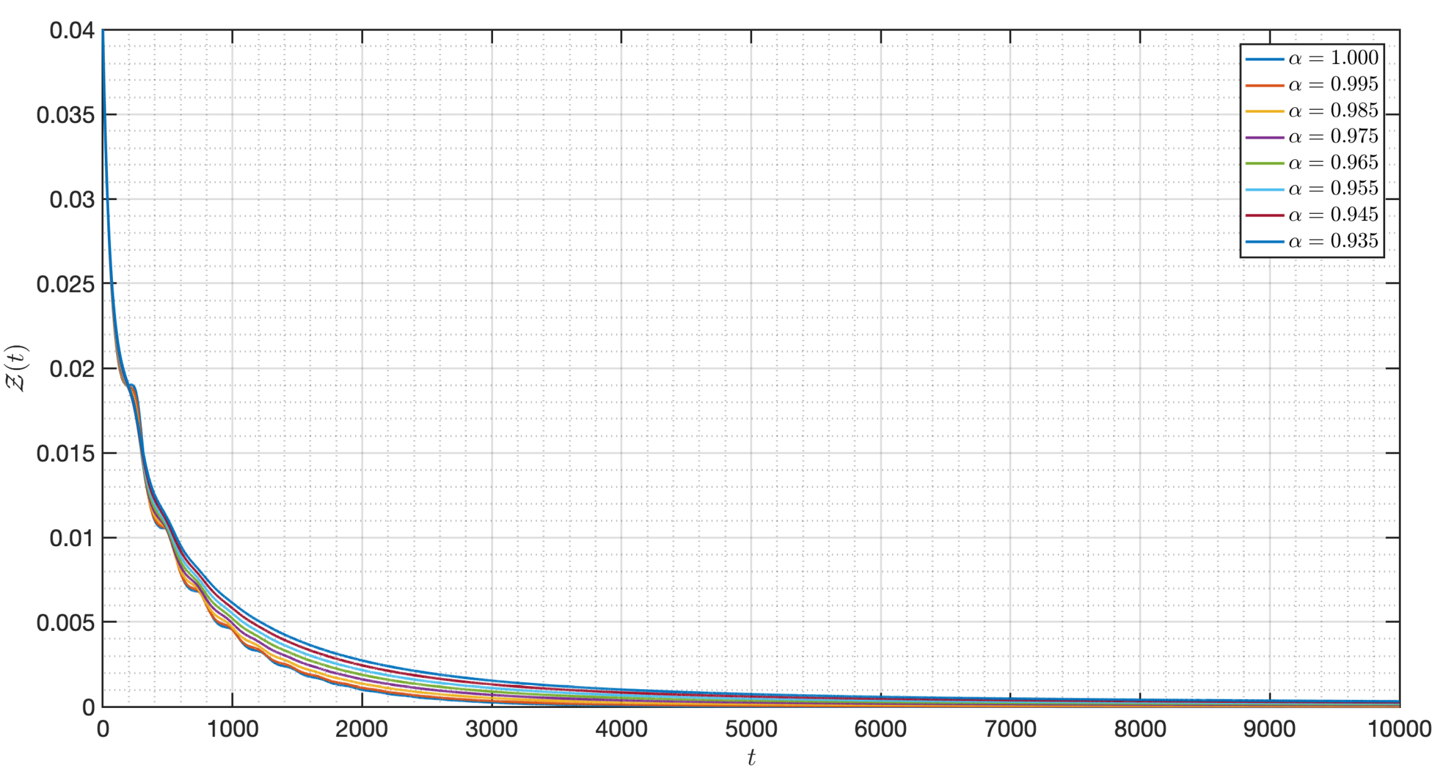
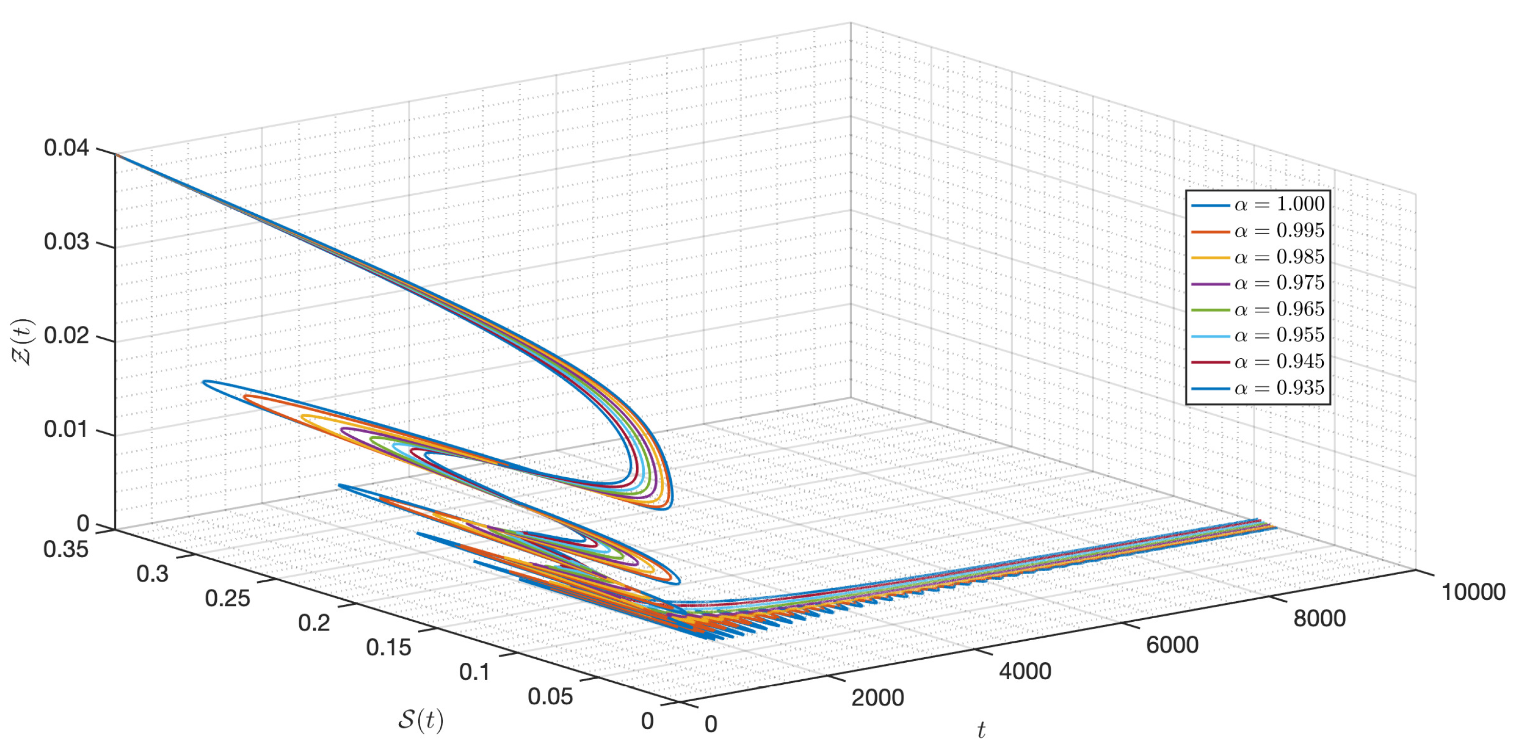
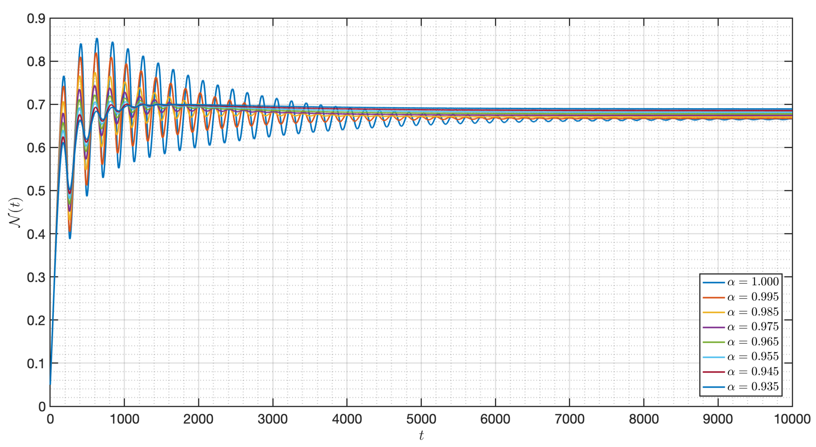
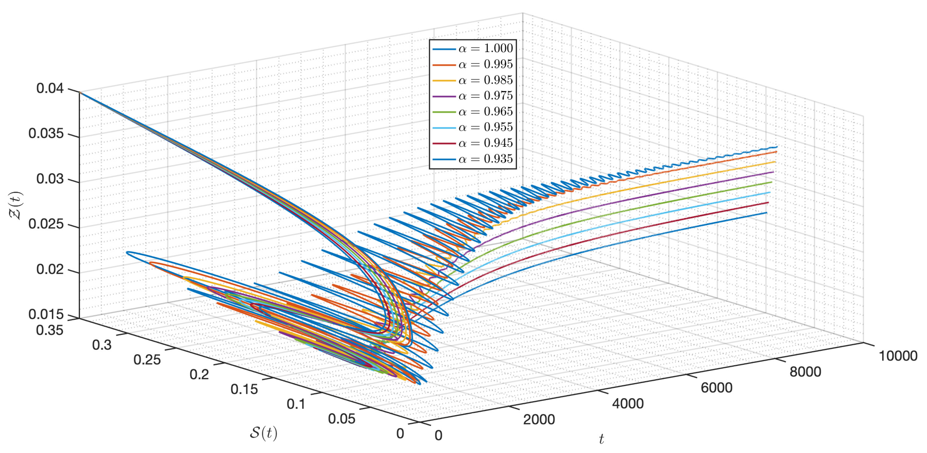
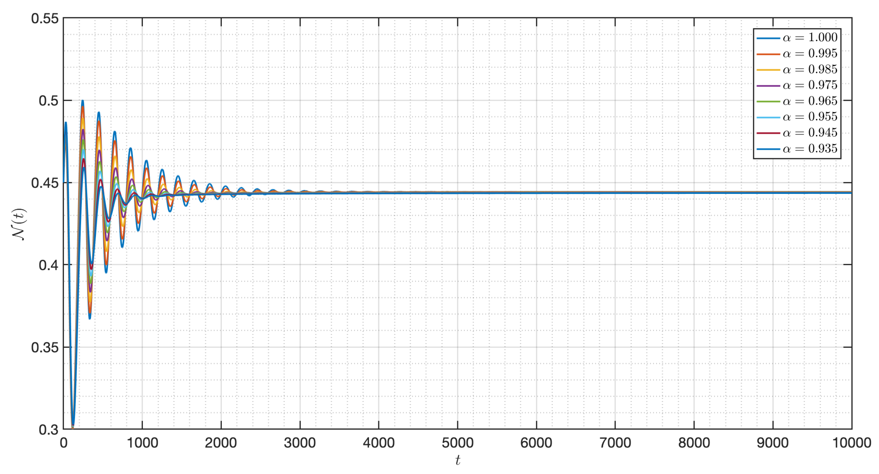
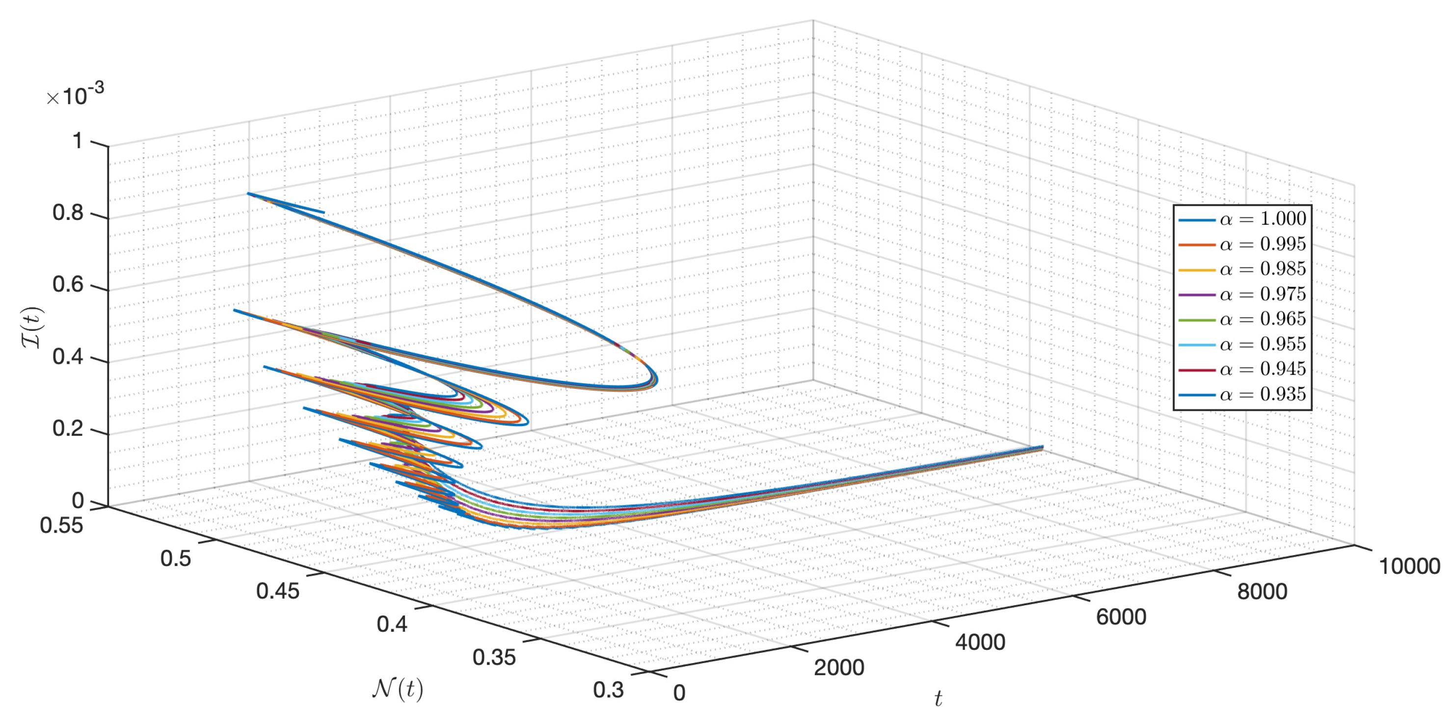
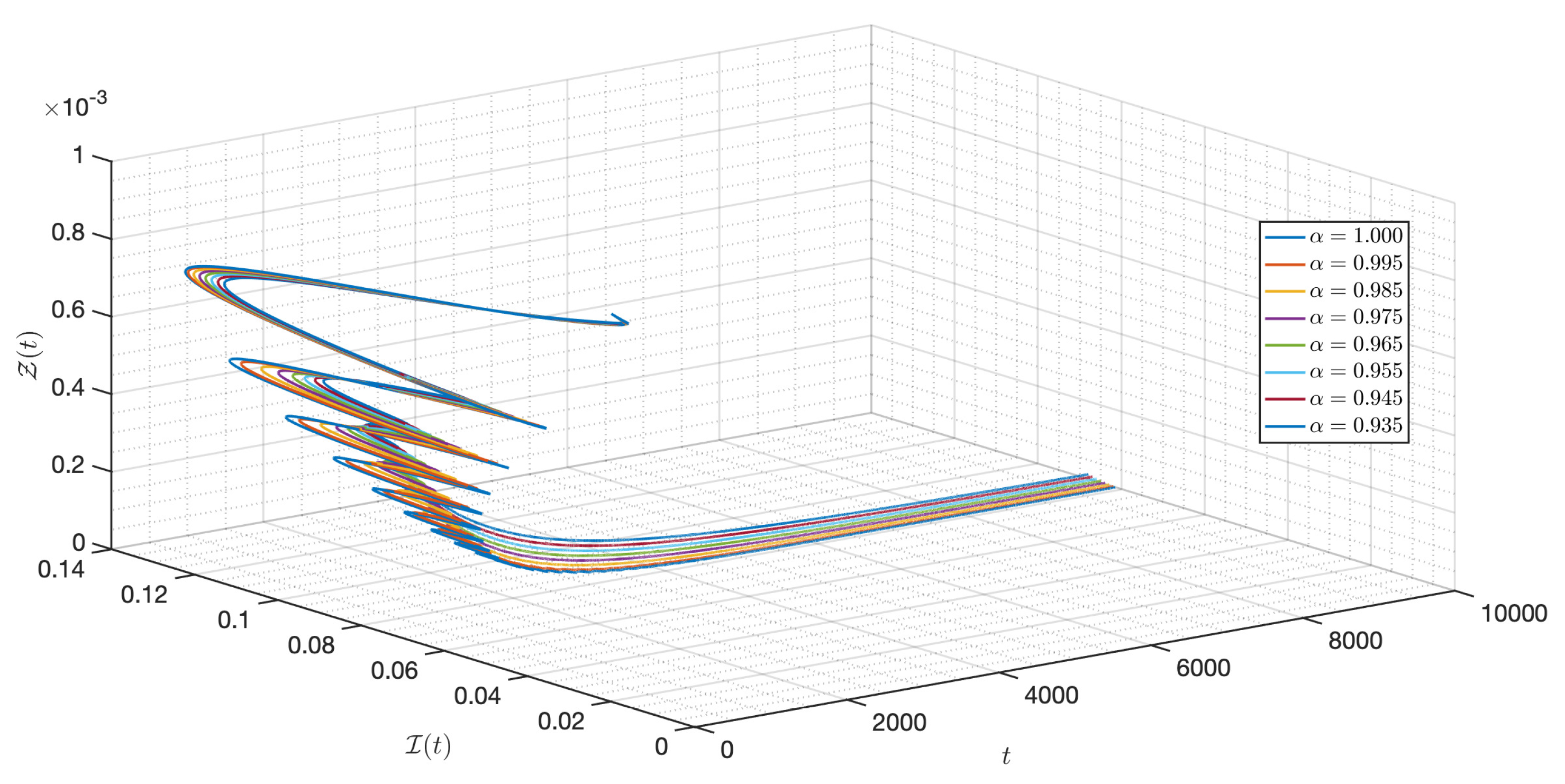
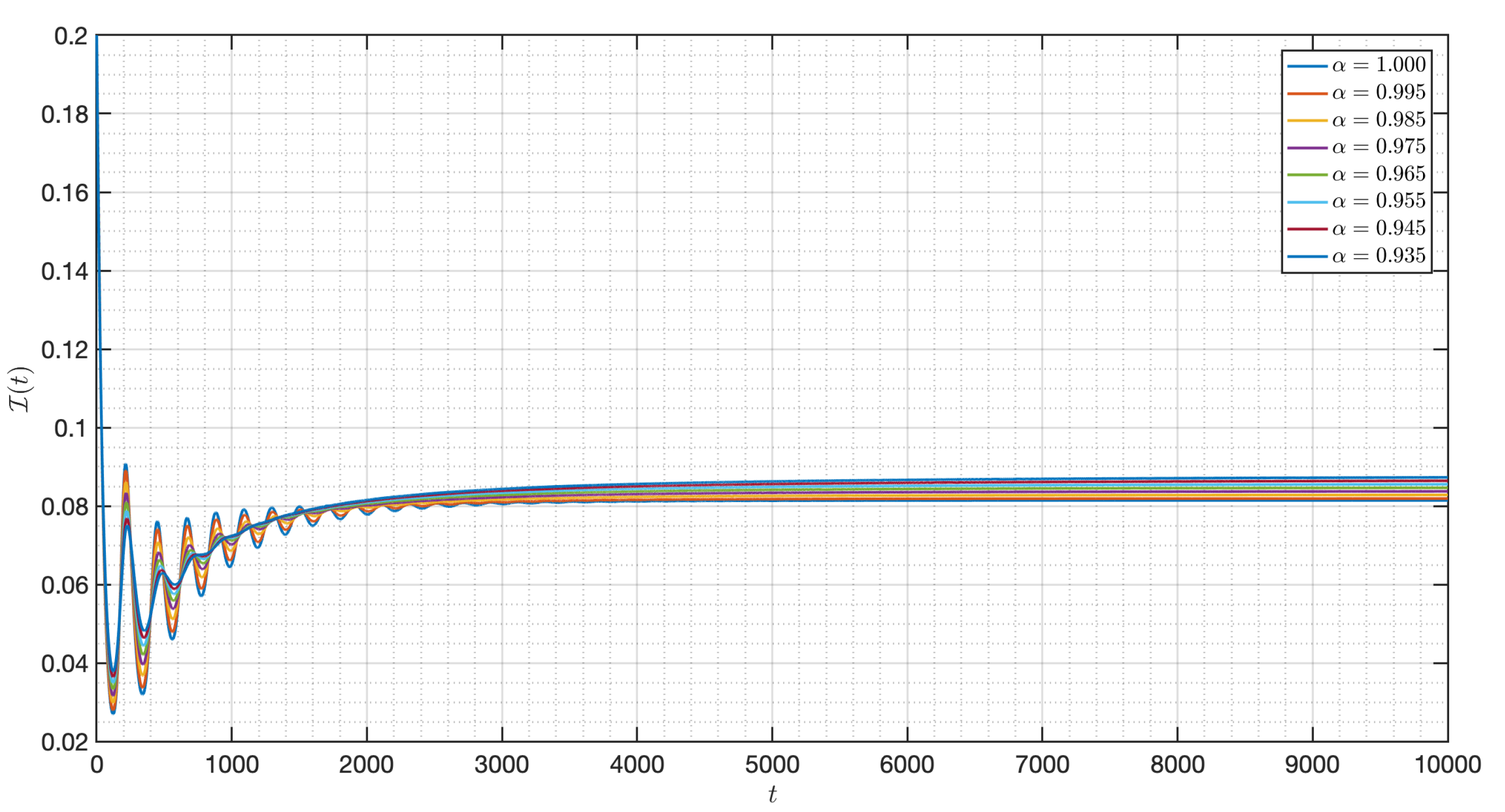
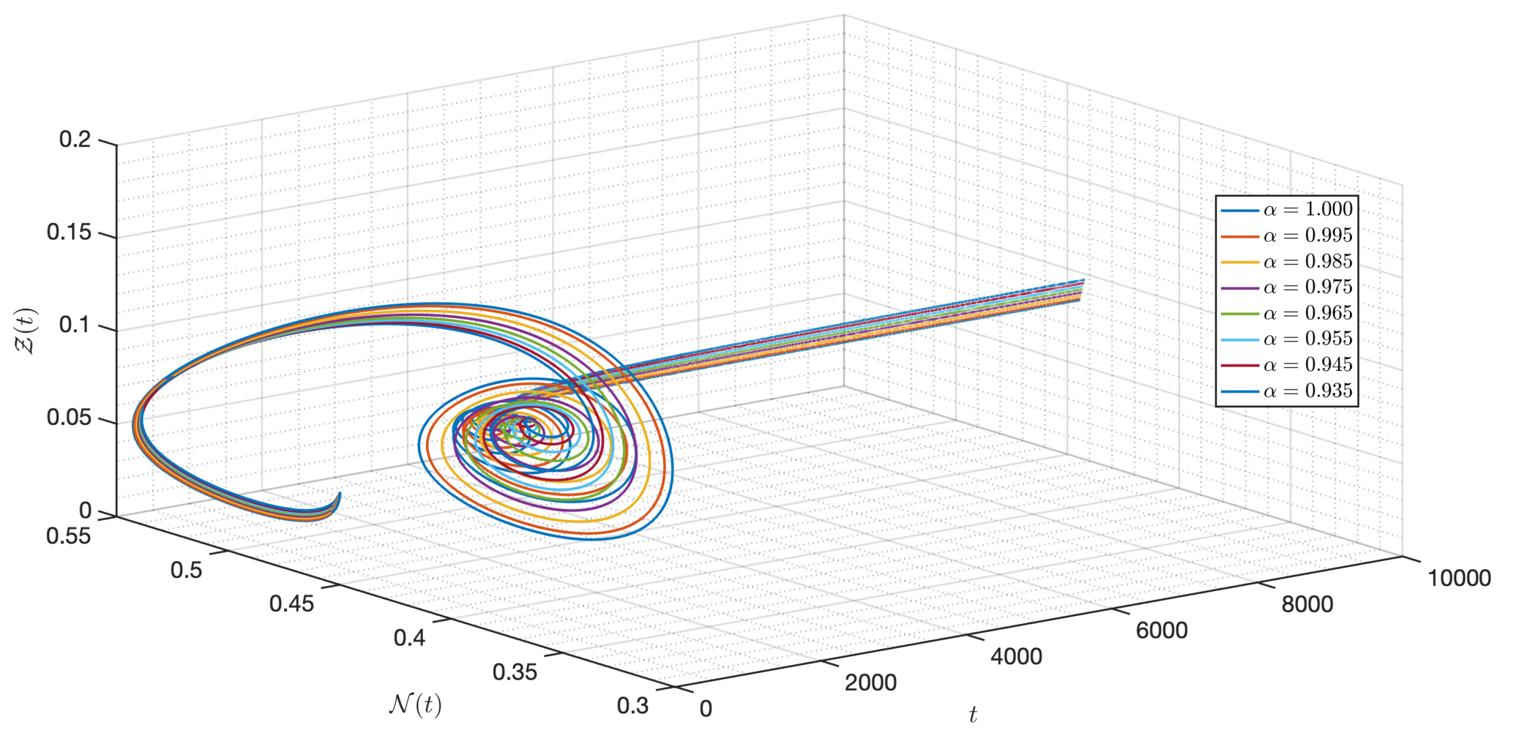
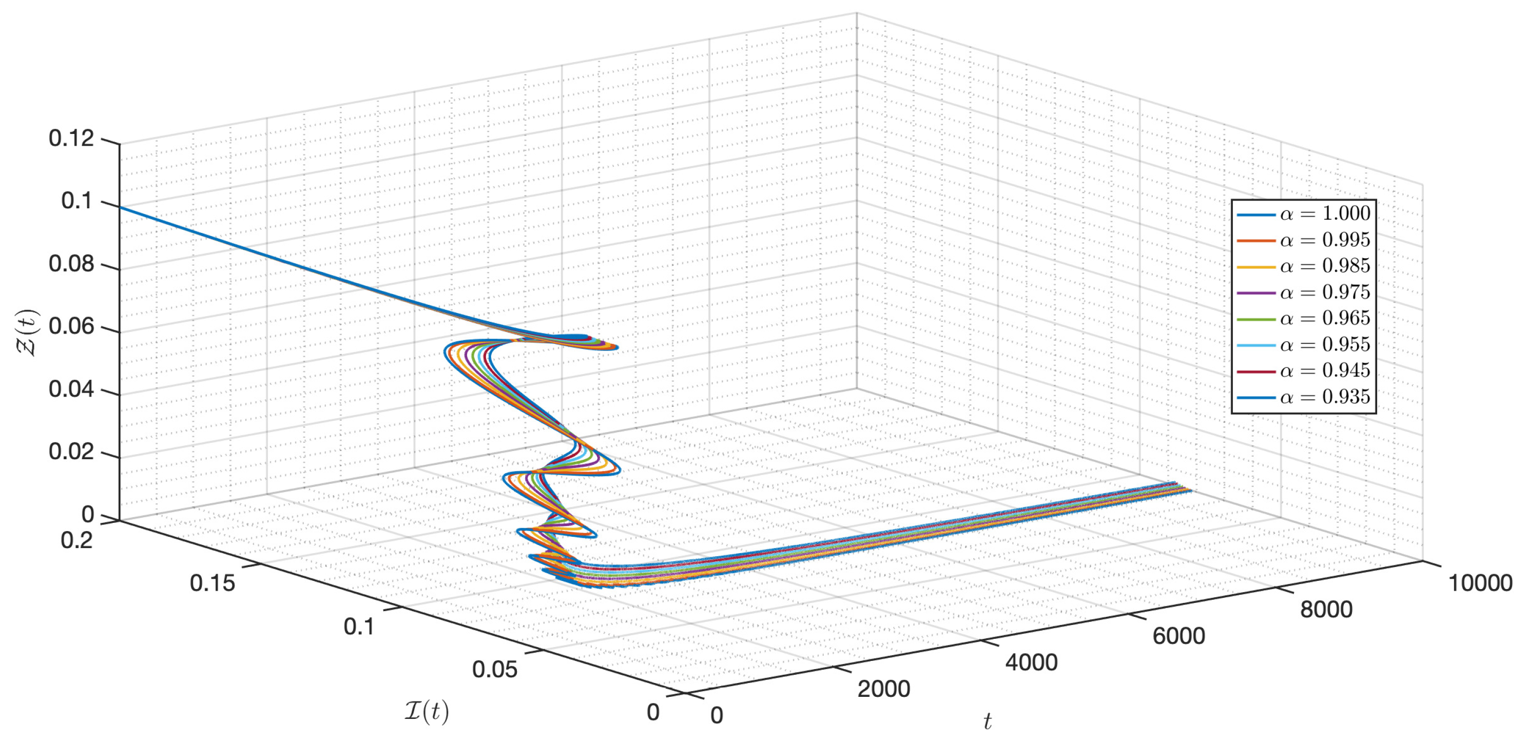
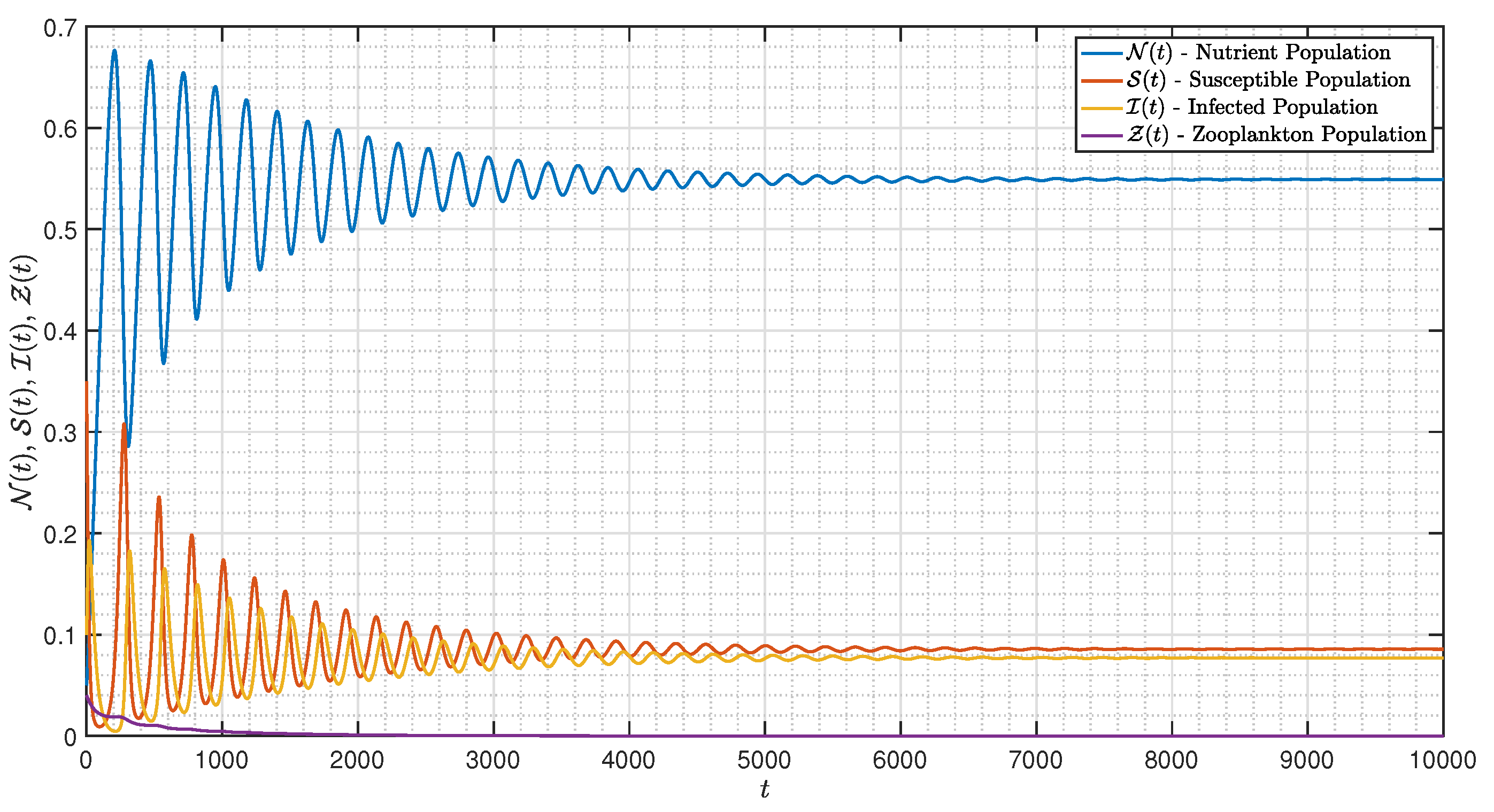
It is shown in Figure 1 that the $\mathbb{ABC}$-$\mathbb{FNPZ}$ model (3) with $\alpha =1.000$ is $\mathcal{LAS}$ around ${\mathfrak{E}}_6^{*}=(0.5491151578,0.08563906497,0.07694268370,0)$. Figure 2, Figure 3, Figure 4, Figure 5, Figure 6, Figure 7, Figure 8, Figure 9, Figure 10 and Figure 11 depict the time series of the system for various fractional orders $\alpha$. Observing the results, the susceptible populations of nutrient, phytoplankton, and infected phytoplankton oscillate increase and decrease until tend to stabilize while the susceptible populations of zooplankton decrease rapidly to zero with different $\alpha$ increase approaching one.

Figure 1. Dynamic of the model (3) for different parameters in Case I with $\alpha =1.000$.

Figure 2. Dynamic of $\mathcal{N}\left(t\right)$ of the model (3) for different order $\alpha$ in Case I.

Figure 3. Dynamic of $\mathcal{S}\left(t\right)$ of the model (3) for different order $\alpha$ in Case I.

Figure 4. Dynamic of $\mathcal{I}\left(t\right)$ of the model (3) for different order $\alpha$ in Case I.

Figure 5. Dynamic of $\mathcal{Z}\left(t\right)$ of the model (3) for different order $\alpha$ in Case I.

Figure 6. Dynamic of the model (3) for different parameters in Case I.

Figure 7. Dynamic of the model (3) for different parameters in Case I.

Figure 8. Dynamic of the model (3) for different parameters in Case I.

Figure 9. Dynamic of the model (3) for different parameters in Case I.

Figure 10. Dynamic of the model (3) for different parameters in Case I.

Figure 11. Dynamics of the model (3) for different parameters in Case I.

Case II. If we set $N_0=5.0$, $\xi =0.0012$, ${\eta }_1=0.02$, ${\eta }_2=0.03$, ${\eta }_3=0.01$, $a=0.1$, $b=0.01$, $c=0.02$, $\beta =0.3$, $m=0.02$, $n=0.04$, $e_1=0.09$, and $e_2=0.07$. Under an initial condition $\left(\mathcal{N}\right(0),\mathcal{S}(0),\mathcal{I}(0),\mathcal{Z}(0\left)\right)=(0.05,0.35,0.10,0.04)$ and

$$\begin{array}{c}\hfill u\left(\mathcal{N}\right)=v\left(\mathcal{N}\right)=w\left(\mathcal{N}\right)=\frac{{\mathcal{N}}^{\alpha }}{1+0.5{\mathcal{N}}^{\alpha }},g\left(\mathcal{S}\right)=\frac{{\mathcal{S}}^{\alpha }}{1+0.5{\mathcal{S}}^{\alpha }},g\left(\mathcal{I}\right)=\frac{{\mathcal{I}}^{\alpha }}{1+0.5{\mathcal{I}}^{\alpha }}.\end{array}$$

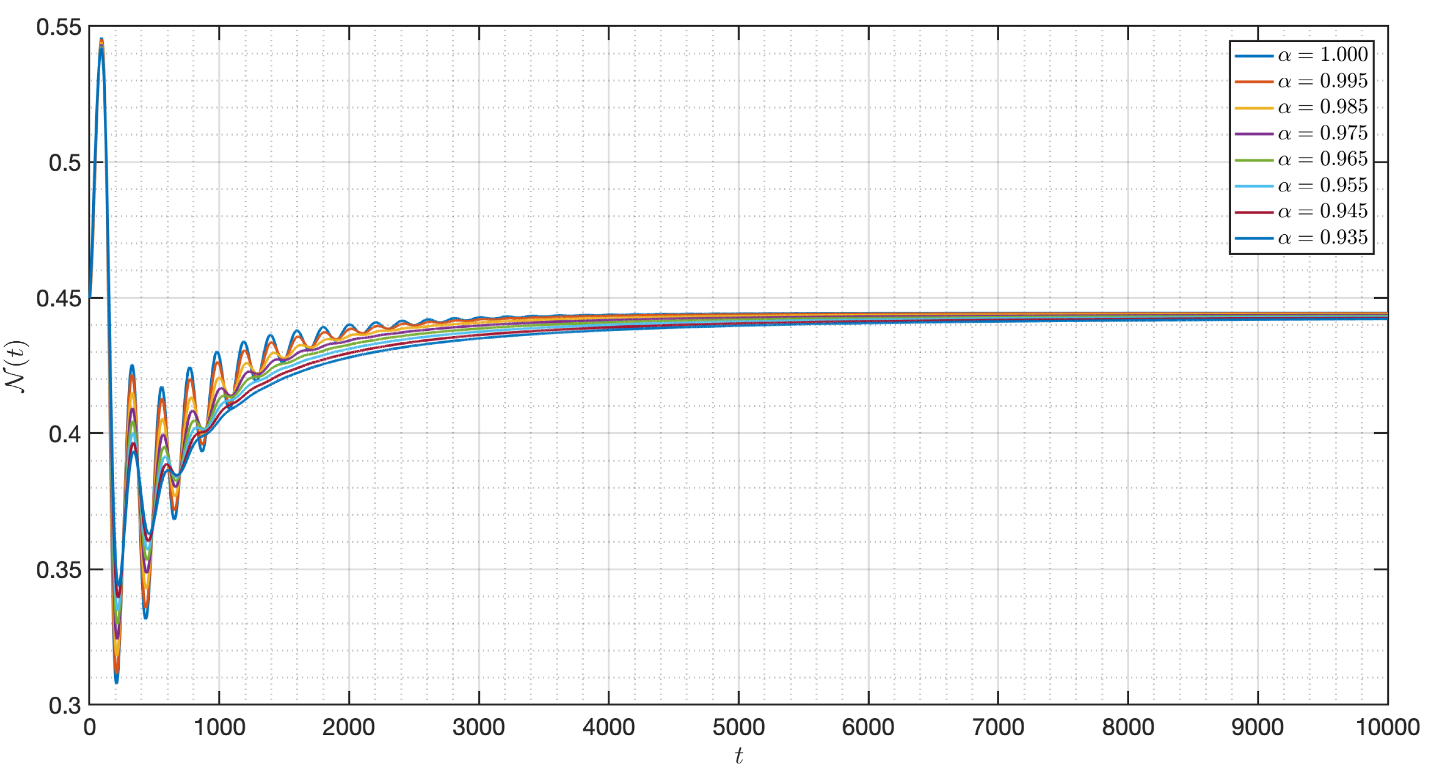
Figure 12 verifies the stability of the system for $\alpha =1.000$. The time series of the system for various fractional orders $\alpha$ are indicated in Figure 13, Figure 14, Figure 15, Figure 16, Figure 17, Figure 18, Figure 19, Figure 20, Figure 21 and Figure 22. In this case, we give the value of $N_0$ different from Case I, so we notice from all figures that the system is $\mathcal{LAS}$ around ${\mathfrak{E}}_7^{*}=(0.6654718801,0.08765044584,0.09761827412$, $0.03378140623)$ where the susceptible populations of nutrient, phytoplankton and infected phytoplankton oscillate increase and decrease until tend to stabilize as well as the susceptible populations of zooplankton a little decrease and increase quickly then tend to stabilize with different $\alpha$ increase approaching one.

Figure 12. Dynamic of the model (3) for different parameters in Case II with $\alpha =1.000$.

Figure 13. Dynamic of $\mathcal{N}\left(t\right)$ of the model (3) for different parameters in Case II.

Figure 14. Dynamic of $\mathcal{S}\left(t\right)$ of the model (3) for different parameters in Case II.

Figure 15. Dynamic of $\mathcal{I}\left(t\right)$ of the model (3) for different parameters in Case II.

Figure 16. Dynamic of $\mathcal{Z}\left(t\right)$ of the model (3) for different parameters in Case II.

Figure 17. Dynamic of the model (3) for different parameters in Case II.

Figure 18. Dynamic of the model (3) for different parameters in Case II.

Figure 19. Dynamic of the model (3) for different parameters in Case II.

Figure 20. Dynamic of the model (3) for different parameters in Case II.

Figure 21. Dynamic of the model (3) for different parameters in Case II.

Figure 22. Dynamic of the model (3) for different parameters in Case II.

Case III. If we set $N_0=3.9$, $\xi =0.0012$, ${\eta }_1=0.02$, ${\eta }_2=0.03$, ${\eta }_3=0.01$, $a=0.1$, $b=0.01$, $c=0.02$, $\beta =0.3$, $m=0.02$, $n=0.04$, $e_1=0.09$, and $e_2=0.07$. Under an initial condition $\left(\mathcal{N}\right(0),\mathcal{S}(0),\mathcal{I}(0),\mathcal{Z}(0\left)\right)=(0.45,0.05,0.02,0.001)$ and

$$\begin{array}{c}\hfill u\left(\mathcal{N}\right)=v\left(\mathcal{N}\right)=w\left(\mathcal{N}\right)={\mathcal{N}}^{\alpha },g\left(\mathcal{S}\right)={\mathcal{S}}^{\alpha },g\left(\mathcal{I}\right)={\mathcal{I}}^{\alpha }.\end{array}$$

In this case, we use the same value of all parameters as in case I but the initial condition and the functional $u\left(\mathcal{N}\right)$, $v\left(\mathcal{N}\right)$, $w\left(\mathcal{N}\right)$, $g\left(\mathcal{S}\right)$, and $g\left(\mathcal{I}\right)$ are changed. As shown in Figure 23, Figure 24, Figure 25, Figure 26, Figure 27, Figure 28, Figure 29, Figure 30, Figure 31, Figure 32 and Figure 33, one of the noticeable aspects of the asymptotic behaviors of the system is the convergence of model solutions to ${\mathfrak{E}}_6^{*}=(0.443037975,0.08518987340,0.08143459917,0)$. The susceptible populations of nutrient, phytoplankton and infected phytoplankton tend to stabilize very fast, while the susceptible populations of zooplankton tend to zero more quickly with different $\alpha$ increase approaching one.

Figure 23. Dynamic of the model (3) for different parameters in Case III with $\alpha =1.000$.

Figure 24. Dynamic of $\mathcal{N}\left(t\right)$ the model (3) for different parameters in Case III.

Figure 25. Dynamic of $\mathcal{S}\left(t\right)$ the model (3) for different parameters in Case III.

Figure 26. Dynamic of $\mathcal{I}\left(t\right)$ the model (3) for different parameters in Case III.

Figure 27. Dynamic of $\mathcal{Z}\left(t\right)$ the model (3) for different parameters in Case III.

Figure 28. Dynamic of the model (3) for different parameters in Case III.

Figure 29. Dynamic of the model (3) for different parameters in Case III.

Figure 30. Dynamic of the model (3) for different parameters in Case III.

Figure 31. Dynamic of the model (3) for different parameters in Case III.

Figure 32. Dynamic of the model (3) for different parameters in Case III.

Figure 33. Dynamic of the model (3) for different parameters in Case III.

Case IV. If we set $N_0=3.9$, $\xi =0.0012$, ${\eta }_1=0.02$, ${\eta }_2=0.03$, ${\eta }_3=0.01$, $a=0.1$, $b=0.01$, $c=0.02$, $\beta =0.3$, $m=0.02$, $n=0.04$, $e_1=0.09$, and $e_2=0.07$. Under an initial condition $\left(\mathcal{N}\right(0),\mathcal{S}(0),\mathcal{I}(0),\mathcal{Z}(0\left)\right)=(0.45,0.05,0.2,0.1)$ and

$$\begin{array}{c}\hfill u\left(\mathcal{N}\right)=v\left(\mathcal{N}\right)=w\left(\mathcal{N}\right)={\mathcal{N}}^{\alpha },g\left(\mathcal{S}\right)={\mathcal{S}}^{\alpha },g\left(\mathcal{I}\right)={\mathcal{I}}^{\alpha }.\end{array}$$

Here, the initial condition differs from Case III. For Figure 34, Figure 35, Figure 36, Figure 37, Figure 38, Figure 39, Figure 40, Figure 41, Figure 42, Figure 43 and Figure 44, we notice that ${\mathfrak{E}}_6^{*}=(0.443037975,0.08518987340,0.08143459917,0)$ is $\mathcal{LAS}$ as well as the behavior of the model quite similar to the other cases as the susceptible populations of nutrient, phytoplankton and infected phytoplankton tend to stabilize, while the susceptible populations of zooplankton tend to zero with different $\alpha$ increase approaching one.

Figure 34. Dynamic of the model (3) for different parameters in Case IV with $\alpha =1.000$.

Figure 35. Dynamic of $\mathcal{N}\left(t\right)$ of the model (3) for different parameters in Case IV.

Figure 36. Dynamic of $\mathcal{S}\left(t\right)$ of the model (3) for different parameters in Case IV.

Figure 37. Dynamic of $\mathcal{I}\left(t\right)$ of the model (3) for different parameters in Case IV.

Figure 38. Dynamic of $\mathcal{Z}\left(t\right)$ of the model (3) for different parameters in Case IV.

Figure 39. Dynamic of the model (3) for different parameters in Case IV.

Figure 40. Dynamic of the model (3) for different parameters in Case IV.

Figure 41. Dynamic of the model (3) for different parameters in Case IV.

Figure 42. Dynamic of the model (3) for different parameters in Case IV.

Figure 43. Dynamic of the model (3) for different parameters in Case IV.

Figure 44. Dynamic of the model (3) for different parameters in Case IV.

As seen in all of the instances above (Case I–IV), the behavior of the system converges to a different steady-state when the parameter values and functions are altered. In these cases, they appear around the equilibrium points ${\mathfrak{E}}_6^{*}$ and ${\mathfrak{E}}_7^{*}$. In addition, the reactions of the system were predicted for various fractional orders, revealing that modest changes in the fractional-order had no effect on the function’s overall behavior, only on the numerical simulations that occur. In addition, we give a few comparisons of our study with the previous studies. It is clear to see that the approximate solutions of the $\mathbb{NPZ}$ model (3) converge to the ordinary solution when fractional-orders $\alpha$ approach one. This means that when $\alpha =1$, the dynamic behavior of the considered system implies exactly the same results as presented in [16]. Moreover, if $u\left(\mathcal{N}\right)=v\left(\mathcal{N}\right)=\mathcal{N}$, $g\left(\mathcal{S}\right)=\mathcal{S}$, $g\left(\mathcal{I}\right)=\mathcal{I}$, and $c=0$, then the $\mathbb{NPZ}$ model (3) is reduced to cover the model presented in [15] for $\alpha =1$.

6. Conclusions

Mathematical modeling using nonlinear differential equations is an important tool for better understanding the behavior of dynamic biological real-world problems. For the summary throughout the manuscript, the $\mathbb{ABC}$–fractional derivative is employed to create the fractional model and the effect of interaction between nutrients, phytoplankton, and zooplankton is investigated. The main aims of this study have been accomplished by proving some theoretical requirements such as the existence and uniqueness with the useful of fixed point theory of Banach’s and Sadovskii’s types. Moreover, the use of Ulam’s stability technique, including $\mathcal{HU}$, $\mathcal{GHU}$, $\mathcal{RHU}$, and $\mathcal{GRHU}$ stability is proved. The accuracy of the theoretical confirmation is verified via the numerical simulations in all diagrams using the Adams’s-type predictor–corrector technique. Based on the results, the non-integer operator used in the study delivers all of the expected theoretical properties of the proposed model and the parameters play an important role in the stability of the ecological system.

It will be a useful alternative technique to apply the $\mathbb{ABC}$-fractional-order derivatives procedure to study and analyze the other diversity of ecological systems in real-world situations for further work. Furthermore, the task remains to develop the results obtained for interesting fractional operators, see [39,40,41].

References

- Kilham, S.S.; Kilham, P. The importance of resource supply rates in determining phytoplankton community structure. In Trophic Interactions Within Aquatic Ecosystems; Meyers, D.G., Strickler, J.R., Eds.; Westview Press Inc.: Boulder, CO, USA, 1984; pp. 7–27. [Google Scholar]
- Smayda, T.J. Species Succession. In The Physiological Ecology of Phytoplankton; Morris, I., Ed.; The University of California Press: Berkeley, CA, USA, 1980; pp. 493–570. [Google Scholar]
- Raymont, J.E.G. Plankton and Productivity in the Oceans; Pergamon Press: London, UK, 1963. [Google Scholar]
- Hecky, R.E.; Kilham, P. Nutrient limitation of phytoplankton in freshwater and marine environments: A review of recent evidence on the effects of enrichment. Limnol. Oceanogr. 1988, 33, 796–822. [Google Scholar] [CrossRef] [Green Version]
- Ryther, J.H.; Dunstan, W.M. Nitrogen, phosphorus, and eutrophication in the coastal marine environment. Science 1971, 171, 1008–1013. [Google Scholar] [CrossRef] [PubMed] [Green Version]
- Lucas, L.V.; Koseff, J.R.; Cloern, J.E.; Monismith, S.G.; Thompson, J.K. Processes governing phytoplankton blooms in estuaries. I. The local production-loss balance. Mar. Ecol. Prog. Ser. 1999, 187, 1–15. [Google Scholar] [CrossRef]
- Berman, T.; Stone, L.; Yacobi, Y.Z.; Kaplan, B.; Schlichter, M.; Nishri, A.; Pollingher, U. Primary production and phytoplankton in Lake Kinneret: A long-term record (1972–1993). Limnol. Oceanogr. 1995, 40, 1064–1076. [Google Scholar] [CrossRef]
- Flynn, K.J.; Fasham, M.J.R.; Hipkin, C.R. Modelling the interactions between ammonium and nitrate uptake in marine phytoplankton. Philosophical Transactions of the Royal Society of London B. Biol. Sci. 1997, 352, 1625–1645. [Google Scholar] [CrossRef]
- Fukuyo, Y.; Takano, H.; Chihara, M.; Matsuoka, K. Red Tide Organisms in Japan-An Illustrated Taxonomic Guide; Uchida Rokakuho, Co., Ltd.: Tokyo, Japan, 1990; p. 401. [Google Scholar]
- Taylor, F.J.R. The species problem and its impact on harmful phytoplankton studies, with emphasis on dinoflagellate morphology. In Toxic Phytoplankton Blooms in the Sea; Smayda, T.J., Shimizu, Y., Eds.; Elsevier: Amsterdam, The Netherlands, 1993; pp. 81–86. [Google Scholar]
- Steidinger, K.A.; Tangen, K. Dinoflagellates. In Identifying Marine Diatoms and Dinoflagellates; Tomas, C.R., Ed.; Academic Press: New York, NY, USA, 1996; pp. 387–598. [Google Scholar]
- Huppert, A.; Blasius, B.; Stone, L. A Model of Phytoplankton Blooms. Am. Nat. 2002, 159, 156–171. [Google Scholar] [CrossRef]
- Singh, B.K.; Chattopadhyay, J.; Sinha, S. The role of virus infection in a simple phytoplankton zooplankton system. J. Biol. 2004, 231, 153–166. [Google Scholar] [CrossRef]
- Chakraborty, S.; Chatterjee, S.; Venturino, E.; Chattopadhyay, J. Recurring Plankton Bloom Dynamics Modeled via Toxin-Producing Phytoplankton. J. Biol. Phys. 2007, 33, 271–290. [Google Scholar] [CrossRef] [Green Version]
- Nath, B.; Roy, P.; Das, K.P. Dynamics of nutrient-phytoplankton-zooplankton interaction in the presence of viral infection. Nonlinear Stud. 2019, 26, 197–217. [Google Scholar]
- Nath, B.; Roy, P.; Sahani, S.K.; Maiti, S.; Das, K.P. Plankton dynamics in nutrient–Phytoplankton–Zooplankton model with viral infection in phytoplankton. Nonlinear Stud. 2020, 27, 1–24. [Google Scholar]
- Rehim, M.; Zhang, Z.; Muhammadhaji, A. Mathematical analysis of a nutrient-plankton system with delay. Springer Plus 2016, 5, 1–22. [Google Scholar] [CrossRef] [PubMed] [Green Version]
- Chakraborty, K.; Dasb, K. Modeling and analysis of a two-zooplankton one-phytoplankton system in the presence of toxicity. Appl. Math. Model. 2015, 39, 1241–1265. [Google Scholar] [CrossRef]
- Wang, Y.; Wang, H.B.; Jiang, W.H. Stability switches and global Hopf bifurcation in a nutrient–plankton model. Nonlinear Dyn. 2014, 78, 981–994. [Google Scholar] [CrossRef]
- Fan, A.; Han, P.; Wang, K. Global dynamics of a nutrient–plankton system in the water ecosystem. Appl. Math. Comput. 2013, 219, 8269–8276. [Google Scholar] [CrossRef]
- Ghanbari, B.; Gómez-Aguilar, J.F. Modeling the dynamics of nutrient-phytoplankton-zooplankton system with variable-order fractional derivatives. Chaos Solit Fractals 2018, 116, 114–120. [Google Scholar] [CrossRef]
- Shi, R.; Ren, J.; Wang, C. Stability analysis and Hopf bifurcation of a fractional order mathematical model with time delay for nutrient-phytoplankton-zooplankton. AIMS 2020, 16, 3836–3868. [Google Scholar] [CrossRef]
- Thabet, S.T.M.; Abdo, M.S.; Shah, K.; Abdeljawad, T. Study of transmission dynamics of COVID-19 mathematical model under ABC fractional order derivative. Results Phys. 2020, 19, 103507. [Google Scholar] [CrossRef]
- Kumar, A.; Baleanu, D. An analysis for Klein-Gordon equation using fractional derivative having Mittag–Leffler-type kernel. Math. Meth. Appl. Sci. 2020, 1–17. [Google Scholar] [CrossRef]
- Rahman, M.; Arfan, M.; Shah, Z.; Alzahrani, E. Evolution of fractional mathematical model for drinking under Atangana-Baleanu Caputo derivatives. Phys. Scr. 2021, 96, 115203. [Google Scholar] [CrossRef]
- Javidi, M.; Nyamoradi, N. A fractional-order toxin producing phytoplankton and zooplankton system. Int. J. Biomath. 2014, 7, 1450039. [Google Scholar] [CrossRef]
- Asl, M.S.; Javidi, M. A new numerical method for solving system of FDEs: Applied in plankton system. Dyn. Contin. Discrete Impuls. Syst. Ser. B Appl. Algorithms 2019, 26, 221–242. [Google Scholar]
- Sekerci, Y.; Ozarslan, R. Dynamic analysis of time fractional order oxygen in a plankton system. Eur. Phys. J. Plus. 2020, 135, 1–13. [Google Scholar] [CrossRef]
- Sekerc, Y.; Ozarlan, R. Oxygen-plankton model under the effect of global warming with nonsingular fractional order. Chaos Solit. Fractals 2020, 132, 109532. [Google Scholar] [CrossRef]
- Ozarlan, R.; Sekerc, Y. Fractional order oxygen-plankton system under climate change. Chaos 2020, 30, 033131. [Google Scholar] [CrossRef]
- Atangana, A.; Baleanu, D. New fractional derivatives with non-local and non-singular kernel: Theory and application to heat transfer model. Therm. Sci. 2016, 20, 763–785. [Google Scholar] [CrossRef] [Green Version]
- Granas, A.; Dugundji, J. Fixed Point Theory; Springer: New York, NY, USA, 2003. [Google Scholar]
- Boyd, D.W.; Wong, J.S.W. On nonlinear contractions. Proc. Am. Math. Soc. 1969, 20, 458–464. [Google Scholar] [CrossRef]
- Zeidler, E. Nonlinear Functional Analysis and Its Application: Fixed Point Theorems; Springer: New York, NY, USA, 1986. [Google Scholar]
- Sadovskii, B.N. A fixed point principle. Funct. Anal. Appl. 1967, 1, 151–153. [Google Scholar] [CrossRef]
- Kongson, J.; Sudsutad, W.; Thaiprayoon, C.; Alzabut, J.; Tearnbucha, J. On analysis of a nonlinear fractional system for social media addiction involving Atangana–Baleanu–Caputo derivative. Adv. Differ. Equ. 2021, 356, 1–29. [Google Scholar] [CrossRef]
- Rus, I.A. Ulam stabilities of ordinary differential equations in a Banach space. Carpath. J. Math. 2010, 26, 103–107. [Google Scholar]
- Alkahtani, B.S.T.; Atangana, A.; Koca, I. Novel analysis of the fractional Zika model using the Adams type predictor–corrector rule for non-singular and non-local fractional operators. J. Nonlinear Sci. Appl. 2017, 10, 3191–3200. [Google Scholar] [CrossRef] [Green Version]
- Valdés, J.E.N. Generalized fractional Hilfer integral and derivative. Contrib. Math. 2020, 2, 55–60. [Google Scholar] [CrossRef]
- Kukushkin, M.V. Abstrac fractional calculus for m-accretive operators. Inter. J. Appl. Math. 2021, 34, 1–41. [Google Scholar] [CrossRef]
- Atangana, A. Fractal-fractional differentiation and integration: Connecting fractal calculus and fractional calculus to predict complex system. Chaos Solitons Fractals 2017, 102, 396–406. [Google Scholar] [CrossRef]
Publisher’s Note: MDPI stays neutral with regard to jurisdictional claims in published maps and institutional affiliations. |
© 2022 by the authors. Licensee MDPI, Basel, Switzerland. This article is an open access article distributed under the terms and conditions of the Creative Commons Attribution (CC BY) license (https://creativecommons.org/licenses/by/4.0/).