Abstract
Image segmentation is a key stage in image processing because it simplifies the representation of the image and facilitates subsequent analysis. The multi-level thresholding image segmentation technique is considered one of the most popular methods because it is efficient and straightforward. Many relative works use meta-heuristic algorithms (MAs) to determine threshold values, but they have issues such as poor convergence accuracy and stagnation into local optimal solutions. Therefore, to alleviate these shortcomings, in this paper, we present a modified remora optimization algorithm (MROA) for global optimization and image segmentation tasks. We used Brownian motion to promote the exploration ability of ROA and provide a greater opportunity to find the optimal solution. Second, lens opposition-based learning is introduced to enhance the ability of search agents to jump out of the local optimal solution. To substantiate the performance of MROA, we first used 23 benchmark functions to evaluate the performance. We compared it with seven well-known algorithms regarding optimization accuracy, convergence speed, and significant difference. Subsequently, we tested the segmentation quality of MORA on eight grayscale images with cross-entropy as the objective function. The experimental metrics include peak signal-to-noise ratio (PSNR), structure similarity (SSIM), and feature similarity (FSIM). A series of experimental results have proved that the MROA has significant advantages among the compared algorithms. Consequently, the proposed MROA is a promising method for global optimization problems and image segmentation.
Keywords:
remora optimization algorithm; multi-level thresholding image segmentation; cross-entropy; meta-heuristic; optimization MSC:
65Y04; 68Q25
1. Introduction
Image segmentation technique is a primary step in computer vision and pattern recognition for pre-processing and analyzing images in the fields of remote sensing, medicine, etc. [1,2,3,4,5]. This technique divides an image into several homogeneous regions or segments with similar characteristics according to features, color, texture, and contrast [6,7]. In the literature, there exist four common types of image segmentation techniques, which can be categorized into (1) region-based techniques, (2) graph-based techniques, (3) clustering-based techniques, and (4) thresholding-based techniques [8]. Among them, the thresholding-based method has gained more attention from researchers due to its efficiency and ease of implementation. The thresholding-based technique can be categorized into bi-level and multi-level thresholding [9]. As the name suggests, the bi-level thresholding uses a single threshold value to segment an image into two homogeneous foreground and background areas. By contrast, multi-level thresholding divides an image into more than two regions based on pixel intensities [10,11,12]. Thus, the multi-level thresholding technique has widely applied in various fields by researchers. However, selecting suitable threshold values is still the most challenging problem and requires further research.
To determine optimal threshold values to segment a given image into several regions, there are two approaches commonly used, which are Otsu’s method (by maximizing between-class variance) and Kapur’s entropy (by maximizing the entropy of the classes) [13]. These methods are suitable for determining a single threshold value. However, when extended into multi-level thresholding, the fatal shortcomings are the computational time and complexity. Therefore, various nature-inspired MAs were proposed in the literature to handle these problems and gained excellent performance [14,15,16].
MAs are considered stochastic algorithms that use randomly generated search agents and specific operators to determine optimal solutions in the search space instead of gradient information. These operators are inspired by nature, such as swarm behavior, social behavior, physics, evolutionary rules, etc. [17,18,19,20,21,22,23,24,25]. Over the last years, various MAs have been proposed and applied in complex real-world problems. Such MAs can be categorized into three main categories: (1) swarm intelligence-based methods, (2) nature evolution-based methods, (3) physics-based methods. The first category mainly simulates the swarm behavior of biological entities, such as birds, slime mould, or the grey wolf. Particle Swarm Optimization (PSO) [26] is one of the most popular MAs inspired by the foraging behavior of birds. Grey Wolf Optimizer (GWO) [27] simulates the grey wolf’s hunting behavior and leadership relationship. Slime Mould Algorithm (SMA) [28] imitates the slime mould’s contraction and oscillation mode during foraging. Other popular MAs in the first category include the Whale Optimization Algorithm (WOA) [29], Cuckoo Search Algorithm (CSA) [30], Salp Swarm Algorithm (SSA) [31], Ant Colony Optimization (ACO) [32], Harris Hawks Optimization (HHO) [33], Moth Flame Optimization (MFO) [34], and Aquila Optimizer (AO) [35]. The second category mainly imitates the evolution process in nature. Genetic Algorithm (GA) [36] is the most famous one developed by the Darwinian evolution law. Some other popular algorithms include Evolutionary Strategy (ES) [37], Differential Evolution (DE) [38], Genetic Programming (GP) [39], Bio-geography-Based Optimizer (BBO) [40], and Evolution Strategy (ES) [41]. The physics-based method simulates the physical laws of the universe. One of the most popular algorithms in this category is Simulated Annealing (SA) [42], which mimics the principle of simulated annealing. It starts from a higher initial temperature, then reduces with the decrease in temperature parameters. Established by this principle, other algorithms include Gravity Search Algorithm (GSA) [43], Gradient-based method (GBO) [44], Sine Cosine Algorithm (SCA) [45], Golden Sine Algorithm (Gold-SA) [46], Arithmetic Optimization Algorithm (AOA) [47], Henry Gas Solubility Optimization (HGSO) [48], Atom Search Optimization (ASO) [49], Central Force Optimization (CFO) [50], and Multi-Verse Optimizer (MVO) [51]. Although many nature-inspired MAs were proposed to solve numerical optimization problems, as real-world problems grow in complexity and difficulty, we need to present more useful MAs to handle them.
Jia et al. [52] presented a new nature-inspired meta-heuristic, namely the Remora Optimization Algorithm (ROA). The main inspiration of ROA is the parasitic behavior of remora during foraging in the ocean. ROA integrates different position update rules based on different hosts. As one of the intelligent creatures in the world, remora usually adsorbs on different hosts to achieve movement and foraging, so the location update rules are the same as those of the host. Moreover, remora also attempt to move by themselves, which is used to determine whether to change hosts. The experimental results demonstrated that the ROA is superior to other algorithms in terms of optimization accuracy and convergence speed. Zheng et al. [53] proposed an improved ROA, namely IROA, for solving global optimization problems. In this work, a mechanism called autonomous foraging was proposed. This mechanism allows each remora a small chance to find the food randomly or according to the current food position, which was used to improve the ROA’s optimization accuracy. Then, the IROA’s performance was evaluated on function optimization and five constrained engineering design problems. The experimental results demonstrated that IROA has a superior performance to other selected MAs in terms of optimization accuracy and convergence speed. However, the No-Free-Lunch (NFL) theorem [54] stated that no unique MAs are available to solve any optimization problems, which encourages us to develop more efficient methods and apply them in various fields such as multi-level thresholding problems.
This paper presents a modified Remora Optimization Algorithm called MROA for global optimization and multi-level thresholding image segmentation tasks. The motivations of this work are to alleviate ROA’s weaknesses and enhance its performance in solving image segmentation tasks. The two major improvements are contained in this work. First, Brownian motion is used to enhance the ROA’s exploration ability and provide it with a high level of opportunity to find the optimal or near-optimal solution in the search space. Second, the lens opposition-based learning strategy is used to improve the exploitation ability of ROA and help search agents to jump out the local optimal solution. We first used 23 benchmark functions in the experimental design including unimodal and multimodal types to validate its performance.
Furthermore, we selected eight grayscale images as the benchmark images, and cross-entropy is employed as the objective function to evaluate the segmentation quality of search agents. We compared MROA with other well-known algorithms and its original in all the tests such as ROA, RSA, AOA, AO, SSA, SCA, and GWO. The experimental results reveal that MROA significantly improved compared with these others in segmentation precision and convergence speed. Overall, it can be proved that MROA is an effective method for global optimization and multi-level thresholding.
The main contributions of this paper can be summarized as follows:
- A new modified ROA, namely MROA, is first proposed based on BM and LOBL strategies.
- The optimization performance of the MROA is evaluated on 23 benchmark functions.
- MROA is applied for thresholding segmentation using the cross-entropy method.
- Validate segmentation quality of MROA in terms of PSNR, SSIM, FSIM, and statistical test.
- The performance of MROA is compared with seven well-known MAs.
The rest of this paper is organized as follows. Section 2 introduces the related work of multi-level thresholding image segmentation using MAs. Section 3 briefly describes the background knowledge. Section 4 presents the proposed MROA. The experimental results are introduced and analyzed in Section 5 and Section 6. Finally, Section 7 concludes this paper and gives future research directions.
2. Related Works
The MAs-based multi-level thresholding segmentation technique has gained more attention from scholars because of its reliable performance, small computational cost, and ease of implementation. In this field, determining the threshold values is the core of the entire segmentation process in the multi-level thresholding technique. In many application scenarios, many scholars use the exhaustive method to determine the optimal threshold values. However, this method has fatal disadvantages, such as complexity, time-consuming computation, and poor threshold values. Therefore, to alleviate these shortcomings, many works show the efficiency and performance of MAs in obtaining optimal threshold values; the following are a few outstanding research works. In [55], Jia et al. presented an efficient satellite image segmentation approach, called DHHO/M, based on dynamic HHO with a mutation mechanism. This work introduces the dynamic control parameter mechanism and mutation operators to improve HHO performance and avoid falling into local optimal solutions. Kapur’s entropy, Otsu between-class variance, and Tsallis entropy were employed to determine optimal threshold values. In the experiments, eight color satellite images and four oil pollution images validate DHHO/M’s performance. The experimental results demonstrated that the DHHO/M provided competitive performance in fitness evaluation, segmentation quality, and statistical tests compared with eight advanced thresholding techniques.
Ewees et al. [56] proposed a new multi-level thresholding method, using modified artificial ecosystem-based optimization (AEO), namely AEODE. The AEODE integrated differential evolution as a local search operator to overcome AEO’s shortcomings. In this way, the AEODE was used to determine a set of optimal threshold values and fuzzy entropy as the objective function. Then, the AEODE was accessed by different grayscale images at six various threshold values. The experimental results show that AEODE outperforms others, including original AEO and DE, in terms of fitness values, PSNR, SSIM, and FSIM.
In [57], an improved version of MPA with an opposition-based learning strategy called MPA-OBL was proposed to determine optimal threshold values at different thresholds. The Otsu between-class variance and Kapur’s were employed as the objective function in this work. The proposed method was evaluated on CEC 2020 test suite and several benchmark images. Compared with ELSHADE-SPACMA-OBL, CMA-ES-OBL, DE-OBL, HHO-OBL, SCA-OBL, SSA-OBL, and standard MPA, the proposed technique MPA-OBL produced better results in different evaluation measurements.
Su et al. [58] presented a variant ABC, namely CCABC, which introduced vertical search and horizontal search mechanisms to improve ABC’s optimization performance. Furthermore, the proposed method, CCABC, was used to find the appropriate threshold values in COVID-19 X-ray images based on Kapur’s entropy. The proposed method was compared with a set of advanced and classical MAs. The evaluation results show that the CCABC is an excellent method in most quality measurements.
Liu et al. [59] proposed a novel multi-level thresholding segmentation technique based on a modified evolution algorithm, called MDE, and applied it to a breast cancer image segmentation task. In this work, the slime mold foraging behavior is introduced to enhance DE’s optimization accuracy and convergence speed. Furthermore, three image quality metrics, including PSNR, SSIM, and FSIM, are used to evaluate its segmentation results to show its segmentation performance.
Li et al. [60] proposed a partitioned and cooperative quantum-behaved particle swarm optimization namely SCQPSO for processing stomach CT images. In this work, SCQPSO was used to determine the optimal threshold values according to Otsu’s method. Additionally, the inter-class variance of Otsu and its variance was used to show SCQPSO’s segmentation quality.
In the literature, we find that more and more scholars presented variants of the multi-level thresholding image segmentation method using MAs to determine optimal threshold values instead of the traditional exhaustive method. Consequently, we confirm that the meta-heuristic-based multi-level thresholding method is a promising work and interesting theories need further research. However, as real-world problems grow in complexity and difficulty, these methods will inevitably fail to find the optimal threshold values during segmentation. Therefore, image segmentation using MAs has more room for improvement to obtain better segmentation quality.
3. Background Knowledge
3.1. Remora Optimization Algorithm (ROA)
ROA [52] is a well-known bionics-based meta-heuristic algorithm inspired by the parasitic behavior of remora during foraging in the ocean. Unlike other fishes, remora usually attach to other hosts (humpback whales or sailfishes) to complete long and short-distance movement in the ocean. Like other MAs, ROA also has three different phases: initialization, exploration, and exploitation.
3.1.1. Initialization
Like other various meta-heuristic algorithms, ROA initializes the search agents using a random approach in the search space, which is calculated by:
where rand denotes a random variable between [0, 1]. ub and lb indicate the search space’s upper and lower bounds. i represents the number of Remora, and N denotes population size.
3.1.2. Free Travel (Exploration Phase)
ROA achieves long-distance and small global movements, respectively, in the search space based on the free travel method. This method includes two main sub-methods: SFO strategy and experience attack.
- SFO strategy
Sailfish: one of the fastest fish in the ocean. Thus, remora attaches to them to achieve quick long-distance movement, and its position update is the same as its host, which is calculated by:
where Xbest(t) indicates global best position of remora and Xrand(t) represents the random position.
- Experience attack
To determine whether the remora changes the host, it needs to take a small step around it. This activity is considered an experience attack and the formula is expressed by:
where Xpre(t) represents the position of the previous generation. randn indicates typically distributed random numbers between 0 to 1.
3.1.3. Eat Thoughtfully (Exploitation Phase)
- WOA strategy
When remora is attached to the humpback whale, its attack strategy is the same as the bubble-net attack strategy in WOA. The mathematical formula can be described as follows:
where D denotes the distance between the best position and current position. α is a random value between [−1, 1].
- Host feeding
This method is a subdivision in the exploitation process. In this phase, remora moving around the host can be thought of as a small step, which can be calculated as follows:
where A denotes a small step movement of remora, which is related to the volume of host and remora. A remora factor (C) is utilized to limit the position of remora to distinguish between the host and remora.
Figure 1 vividly illustrates the main process of ROA, and the pseudo-code of ROA is presented in Algorithm 1.
| Algorithm 1 the pseudo-code of ROA |
|
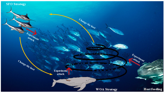
Figure 1.
The different process of ROA.
3.2. Brownian Motion
Brownian motion (BM) is a stochastic process in which step length is drawn from the probability function defined by a normal distribution with zero mean (μ = 0) and unit variance (σ2 = 1) [61,62]. The probability density function at point x for BM is calculated via:
where x indicates a point following this motion and the distribution, 2D, and 3D trajectory of BM as shown in Figure 2. As the related figures show, we can see that BM can over areas of the domain with more uniform and controlled steps in the search space. On the other hand, BM’s trajectory can trace and explore distant areas of the neighborhood.
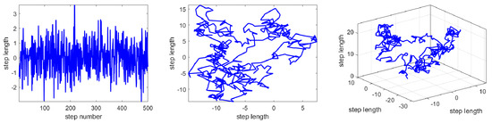
Figure 2.
Brownian distribution, 2D Brownian trajectory, and 3D Brownian trajectory.
3.3. Lens Opposition-Based Learning
Lens opposition-based learning (LOBL) [63] is a novel strategy that integrates both opposition-based learning (OBL) [64] strategy and lens imaging principle to enhance the searchability of MAs. The LOBL strategy shows more effective performance during the optimization process than OBL when finding optimal or near-optimal solutions in the search space. The mathematical principle of LOBL is described as follows:
Lens imaging theory illustrates that when the distance from the object to the lens exceeds two times the focal length, an inverted and constricted real image will be formed between 1–2 times the focal length on the other side of the lens. As shown in Figure 3, where O represents the midpoint of the interval [lb, ub] and the y-axis is treated as a convex lens. In addition, an object of height h is located at point x, which is twice the lens’s focal length. Through lens imaging, the coordinates of the image vertices become (x*, h*). The formula is listed as follows:
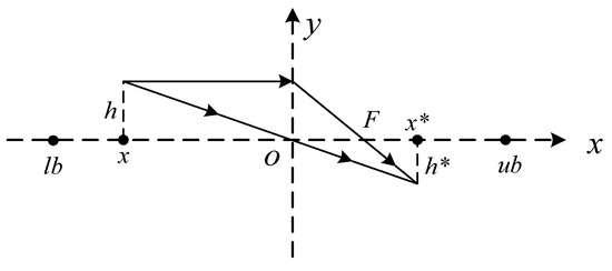
Figure 3.
Diagram of LOBL.
Let k = h/h*, Equation (14) can be simplified as follows:
In general, the optimization tasks are multi-dimensional, so the Equation (15) can be extended as follows:
where denotes the opposite point of in i-th dimension. Interestingly, if k = 1, Equation (16) is the same as the OBL strategy. Therefore, the LOBL can be considered as a variant of OBL. The difference is that LOBL used an adjusting parameter k to realize dynamic search behavior when solving optimization tasks, which further improves the probability of the algorithm escaping from the local optimal solution.
3.4. Cross Entropy
In 1968, cross-entropy was proposed by Kullback [65]. As an essential concept in Shannon’s information theory, cross-entropy is mainly used to measure the difference in information between two probability distributions [66,67]. Let P = {p1, p2, …, pn} and Q = {q1, q2, …, qn} be two probability distributions defined over the same set of values. The cross-entropy between P and Q can be calculated as follows:
The minimum cross-entropy algorithm determines the threshold value by minimizing the cross-entropy between the original image and the thresholded image [68]. The lower the cross-entropy value, the lower the uncertainty and the greater the homogeneity. Let the original image be I, and h(i), i = 1, 2, …, L, is the corresponding histogram with L being the number of grey levels. Then the thresholded image Ith is created by the threshold value th using the following equations:
The thresholded image is generated based on Equation (17), then we can calculate the cross-entropy by rewriting Equation (17) as an objective function (also called fitness), which is listed below:
The above objective function considers a single threshold value to segment a given image, i.e., bi-level thresholding, it also can be extended to a multi-level approach for image segmentation, called multi-level thresholding image segmentation. Thus, the Equation (19) can be expressed as:
where th = [th1, th2, …, thnt] indicates an array containing nt different threshold values. Hi is defined as follows:
4. The Proposed Algorithm
4.1. The Details of MROA
Although ROA is easy to implement, suitable for solving optimization tasks widely, and provides more reliable results than other Mas, it has insufficient searchability (exploration and exploitation) in solving complex optimization problems; for example, it easily stagnates into optimal local solutions and has a slow convergence speed. Motivated by these considerations, this paper proposes a modified ROA algorithm called MROA for global optimization and multi-level thresholding image segmentation. There are two major strategies for modifying. First, Brownian motion is introduced to improve the exploration ability and provide a greater opportunity to find the optimal or near-optimal solution in the search space. Second, LOBL is used to improve the exploitation ability and accelerate the convergence rate of ROA. Therefore, the exploration phase of ROA is modified using Brownian motion, which is expressed as:
where Brownian indicates Brownian motion.
The pseudo-code of MROA is presented in Algorithm 2, and Figure 4 illustrates the flowchart of MROA.
| Algorithm 2 the pseudo-code of MROA |
|
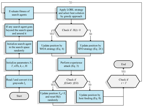
Figure 4.
Flowchart of the proposed MROA.
4.2. The Proposed MROA for Solving Multi-Level Thresholding Image Segmentation Task
In this subsection, the MROA is employed to solve the multi-level thresholding image segmentation task and cross-entropy is used to determine optimal threshold values. We present the different steps of this method as below:
Step 1: Read image I and convert it to grayscale Ig, calculate the histogram h of Ig.
Step 2: Initialize the parameters of MROA: N, T, C, k, and random array H.
Step 3: Initialize the location of search agents with N population size and nTh dimensions.
Step 4: If any search agent goes beyond the search space and amend it.
Step 5: Evaluate the cross-entropy with Equation (20) for each search agent.
Step 6: Apply LOBL strategy to generate lens opposite solution and select the best one between the original and its opposite solution according to the fitness value.
Step 7: Select the appropriate host to update the location of the search agent according to the value of the H.
Step 8: The t index is increased in 1, if the stop criteria (t ≥ T) are satisfied then output the best threshold values, otherwise jump to Step 5.
Step 9: Generate the segmented image Seg with the best threshold values obtained by MROA.
4.3. Computation Complexity of MROA
In the initialization phase, MROA produces the search agents randomly in the search space, so the computational complexity of this phase is O(N × D), where N denotes the number of population and D denotes the dimension size. Afterward, MROA evaluates each individual’s fitness during the whole iteration with the complexity O(T × N × D), where T indicates the number of iterations. Finally, for position updating, the complexity is summarized as O(T × N × D). In summary, the total computational complexity of MROA is O(T × N × D), which is the same as the original.
5. Experimental Results for Global Optimization
This section evaluates the optimization performance of the proposed MROA using 23 benchmark functions. First, the definitions of the 23 benchmark functions are introduced. Second, the experimental setup and comparison group including other well-known MAs are described in detail. Finally, the experimental results are analyzed and discussed.
5.1. Definition of 23 Benchmark Functions
To evaluate the searchability of the proposed MROA, 23 benchmark functions are introduced in this paper [15]. These functions are categorized into: (1) unimodal functions (F1–F7), (2) multimodal functions (F8–F14), and (3) fixed-dimension multimodal functions. These functions are defined in Table 1, where D, UM, and MM indicate the dimension, unimodal, and multimodal functions, respectively. Figure 5 shows the visualization of these functions. We can see that the unimodal functions have only one global optimal solution, which is available to evaluate the exploitation ability of MAs. By contrast, multimodal and fixed-dimension multimodal functions have many local optimal and only one global optimal solution, which is available to evaluate the exploration and ability to escape from the local optimal solution of MAs.

Table 1.
Definition of 23 benchmark functions.
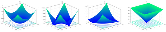
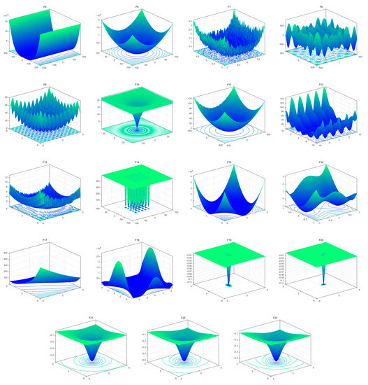
Figure 5.
View of 23 benchmark functions.
5.2. Experimental Setup
As stated above, the 23 benchmark functions are utilized to evaluate the optimization performance of the proposed work. To show the representativeness of experimental results, the proposed algorithm MROA is compared with the original ROA [52] and other well-known MAs, including RSA [69], AOA [47], AO [35], SSA [31], SCA [45], and GWO [27]. For fair evaluation, we set the number of maximum iteration T = 500, population size N = 30, and dimension size D = 30, respectively. Moreover, all the tests are run 30 times independently. The best results are highlighted in bold. Table 2 represents the parameter setting of each algorithm and the details of these algorithms are listed as follows:
- ROA [52]: Simulates remora’s parasitic behavior on hosts, such as whales and swordfish, to finish the predation behavior.
- RSA [69]: mimics the encircling and hunting mechanism of a crocodile swarm during foraging.
- AOA [47]: simulates the behavior of arithmetic operators in nature, which include multiplication (×), division (÷), addition (+), subtraction (−).
- AO [35]: inspired by the different hunting behavior of Aquila hawks in nature.
- SSA [31]: simulates the swarming behavior of salps during moving and foraging in the ocean.
- SCA [45]: simulates the common mathematical models, sine and cosine functions.
- GWO [27]: mimics the hunting strategy and leadership hierarchy of gray wolves.
Table 2.
Parameter settings for each algorithm.
Table 2.
Parameter settings for each algorithm.
| Algorithm | Parameters |
|---|---|
| MROA | c = 0.1; k = 10,000 |
| ROA [52] | c = 0.1 |
| RSA [69] | α = 0.1; β = 0.1 |
| AOA [47] | α = 5; μ = 0.5; |
| AO [35] | U = 0.00565; c = 10; ω = 0.005; α = 0.1; δ = 0.1; |
| SSA [31] | c1 = [1, 0]; c2 ∈ [0, 1]; c3 ∈ [0, 1] |
| SCA [45] | A = 2 |
| GWO [27] | a = [2, 0] |
5.3. Statistical Results on 23 Benchmark Functions
This subsection compared MROA with seven basic algorithms on 23 benchmark functions in terms of the mean value (Mean) and standard deviation (Std). The experimental results are given in Table 3. By observing this table, we can see that MROA has the smallest Mean and Std values among the most functions. Specifically, for F1–F4, MROA obtains the theoretical optimal solution, where ROA only finds the optimal solution, which shows the LOBL strategy effectively enhances the exploitation ability of MROA, and the lens opposite solution increases the diversity of the population, helping the search agents to jump out of the local optimal solution. For MM functions, MROA also provides more competitive results than seven well-known algorithms; the Brownian motion strategy improves the ROA’s exploration capability and provides search agents with a greater opportunity to find the optimal or near-optimal solution in the search space. For F8, although MROA only finds the near-optimal solution, its convergence accuracy is also better than others. For F9, F10, and F11, MROA obtains the theoretically optimal solution. For F12, F13, and F4, the accuracy of MROA is weaker than AO and SSA, respectively. For F15–F23, MROA also provides a higher convergence accuracy than others. Moreover, Figure 6 shows the MROA and competitor algorithms’ ranking in UM and MM functions. We can see from the results that the proposed MROA outperforms in most benchmark functions.
Table 3.
Statistical results of algorithms on 23 benchmark functions.
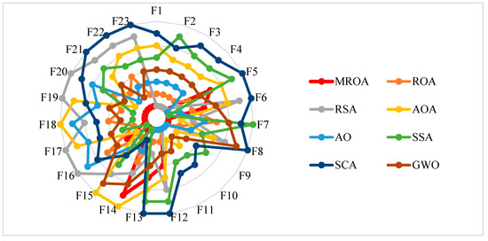
Figure 6.
The radar graphs of algorithms on 23 benchmark functions.
Furthermore, owing to the MAs being stochastic algorithms, in this paper, we consider the Wilcoxon rank-sum test to supplement our statistical analysis and evaluate the statistical significance of the results [70]. The Wilcoxon rank-sum test is a non-parametric test used to compare the results of each pair of algorithms. The test is based on two hypotheses: null and alternative. The null hypothesis indicates that there is no difference between the two samples. The alternative hypothesis indicates that there is a significant difference between the two samples. We set the significance level as 5%; according to this criterion, if the p-value is higher than 0.05, which indicates the null hypothesis is true, the significant difference is not obvious. If the p-value is less than 0.05, which indicates there is a significant difference, the null hypothesis is rejected. Furthermore, NaN denotes that there is no difference between the two samples. Table 4 shows the p-values obtained using the Wilcoxon rank-sum test, which is calculated by the fitness values between MROA and each of the algorithms included, presenting six different pairs, MROA vs. ROA, MROA vs. RSA, MROA vs. AOA, MROA vs. AO, MROA vs. SSA, MROA vs. SCA, and MROA vs. GWO. This table shows that the results of MROA are statistically significant for most benchmark functions, which indicates that the performance of MROA is not random. Consequently, based on the above analysis, we conclude that the MROA outperforms other algorithms for most benchmark functions in terms of convergence accuracy and statistical significance.
Table 4.
Statistical results of algorithms on 23 benchmark functions using Wilcoxon rank-sum test.
5.4. Boxplot Behavior Analysis
To further validate the excellent performance of the proposed MROA, Figure 7 presents the boxplot behavior of MROA and other MAs for some functions, including UM and MM types. Since boxplots indicate the data distribution, it is available to describe the consistency between data. MROA is very narrow compared with other algorithms and maintains the lowest values for most functions. It is observed that ROA outperforms the other algorithms in terms of data distribution, but only on F6, F8, and F15; the performance is mediocre for data distribution.
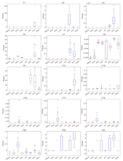
Figure 7.
Boxplot behavior of algorithms on some functions.
5.5. Convergence Behavior Analysis
This subsection analyzed the convergence behavior of the proposed MROA with compared algorithms. The convergence curve of these algorithms on 23 benchmark functions is shown in Figure 8. From this figure, we can conclude that MROA outperforms other well-known MAs in terms of convergence speed and optimization accuracy. For unimodal functions F1, F2, and F4, MROA achieves the fastest convergence speed and obtains the theoretically optimal solutions. However, for F6, the performance of MROA is not excellent and it may be trapped into the local optimal. For F7, although MROA cannot obtain the theoretical optimal solution, it also finds the most near-optimal solution and shows the fastest convergence speed than others. For MM functions, MROA also shows excellent optimization performance than other popular methods. For F8, MROA has a significant convergence capability that exceeds two ROA and SSA methods. For F9 and F11, MROA finds the theoretical optimal solution and has a faster convergence speed than others. We concluded that MROA has an excellent convergence ability in UM and MM functions.
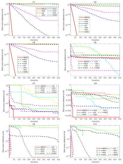
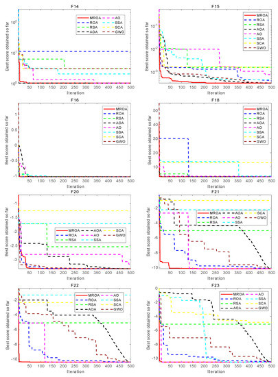
Figure 8.
Convergence behavior of algorithms on some functions.
6. Experimental Results for Multi-Level Thresholding Image Segmentation
This section used MROA to minimize the cross-entropy for solving multi-level thresholding image segmentation tasks. First, we selected eight images from the Berkeley segmentation dataset [71] as the benchmark images and the experimental setup described in detail. Second, three image measurements, including PSNR, SSIM, and FSIM are introduced to measure the segmentation performance (quality, consistency, and accuracy) of MROA and other algorithms. Finally, the experimental results are discussed and analyzed.
6.1. Berkeley Segmentation Dataset
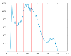
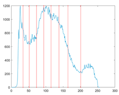
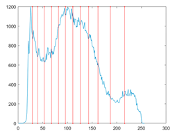
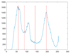
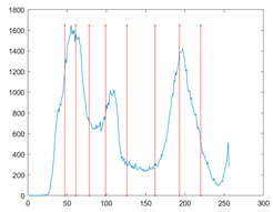
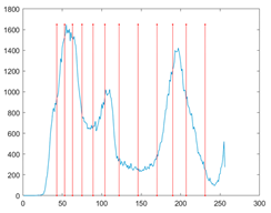
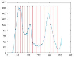
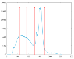
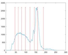
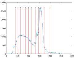
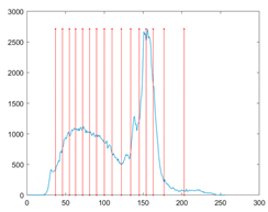
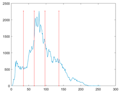
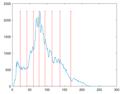
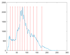
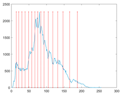
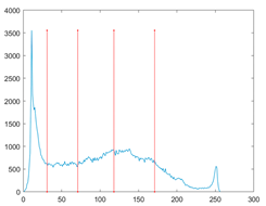
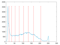
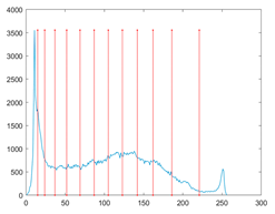
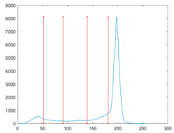
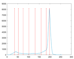
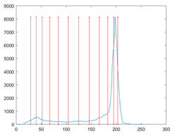
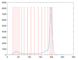
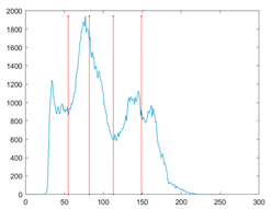
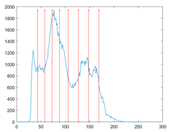
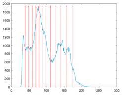
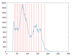
The proposed MROA with other algorithms is evaluated on eight images from the Berkeley segmentation dataset [71]. In this work, eight benchmark images are grayscale. These images and their histogram are presented in Figure 9. The purpose of selecting these images is only to test the algorithms’ segmentation performance and quality.
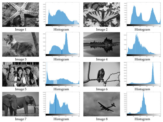
Figure 9.
Berkeley image dataset and its histogram.
6.2. Experimental Setup
The proposed MROA is compared with seven well-known algorithms such as ROA [52], RSA [69], AOA [47], AO [35], SSA [31], SCA [45], and GWO [27]. The described parameters and settings of these algorithms are described in Section 4.2. For fair evaluation, the number of maximum iteration T = 500, the population size N = 30, and all the algorithms were run 30 times independently. The best values are highlighted in bold. All the images are segmented using different threshold values nTh = [4, 8, 12, 16].
6.3. Segmentation Quality Evaluation Measurements
6.3.1. Peak Signal-to-Noise Ratio (PSNR)
PSNR is used to calculate the ratio between the maximum possible signal power and the distorted noise power that affects the quality of its representation. The signal is regarded as the original data, and the noise is the error caused by segmentation. The PSNR is the most commonly used quality assessment technique to compare an original image and its segmented images using root mean square error (RMSE) per pixel. A higher PSNR indicates more similarity between the images, which is reflected in a better segmentation process [71,72]. It can be described as follows:
where Ig and Seg denote the original and segmented image, respectively. M and N are the sizes of the image.
6.3.2. Structural Similarity (SSIM)
The SSIM is used to measure the degree of distortion of the images, and it can also measure the similarity from three perspectives, including luminance, contrast, and structural content between original and segmented images. Unlike mean-square error (MSE) and PSNR, SSIM measures absolute error, which is more in line with the intuitive feeling of the human eye [72,73]. SSIM is computed by the following equation:
where μI and μSeg indicate the mean intensities of the original and its segmented image, respectively. σI and σSeg are standard deviations of original and its segmented images. σI, Seg is the covariance between original and segmented images. c1 and c2 are two constants equal to 0.065.
6.3.3. Feature Similarity (FSIM)
FSIM is a variant of SSIM that considers low-level features such as the gradient magnitude and phase congruency to measure the similarity of two images [74,75]. It can be described as follows:
where Ω indicates the entire domain of the image. T1 and T2 are constants which equal to 0.85 and 160, respectively. G indicates the gradient magnitude of an image, and PC denotes the phase congruence.
6.4. Experimental Results Analysis of Benchmark Images
We compared MROA with other well-known algorithms for solving multi-level thresholding image segmentation tasks in this subsection. Cross-entropy is used as the objective function. Table A1 (in Appendix A) denotes the best threshold values obtained by algorithms at different threshold values. Table A2 contains the segmented images obtained from the proposed MROA at nTh = [4, 8, 12, 16]. Table A3, Table A4, Table A5 and Table A6 show the mean and standard deviation values for fitness, PSNR, SSIM, and FSIM obtained by algorithms, respectively. The higher mean values obtained indicate more optimization accuracy and efficiency of an algorithm.
On the other hand, the smaller the standard deviation values, the more stable the algorithm. Table A7 shows the Wilcoxon rank-sum results for fitness, the significance level is the same as Section 4.3. Moreover, Figure 10, Figure 11, Figure 12 and Figure 13 show the summary average results obtained by algorithms in terms of fitness, PSNR, SSIM, and FSIM, respectively. Figure 14 summarized the best cases in terms of fitness, PSNR, SSIM, and FSIM, respectively.
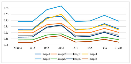
Figure 10.
Average fitness values obtained by the algorithms over all images.
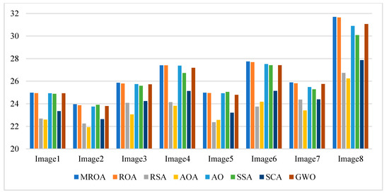
Figure 11.
Average PSNR values obtained by the algorithms over all images.
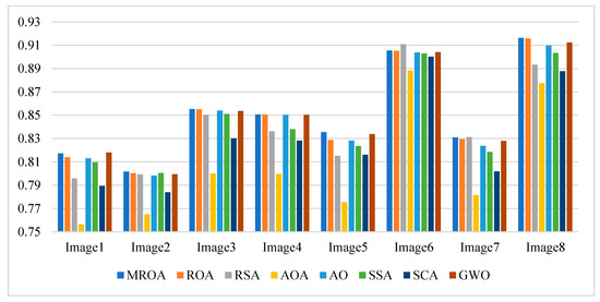
Figure 12.
Average SSIM values obtained by the algorithms over all images.
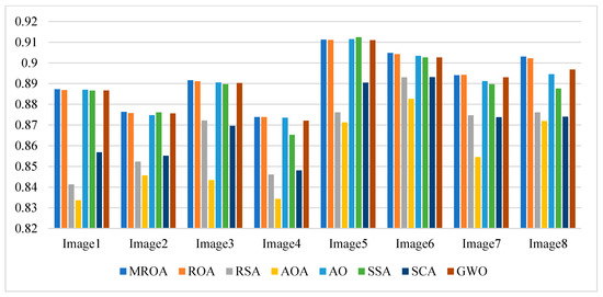
Figure 13.
Average FSIM values obtained by the algorithms over all images.
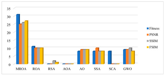
Figure 14.
The number of best cases based on the fitness, PSNR, SSIM, FSIM obtained by algorithms over all images.
It can be seen from Table A1 that in most cases, when the threshold level is 4 and 8, similar values are obtained by algorithms, especially for ROA, AO, SSA, and GWO. When the threshold level is 12 and 16, the difference is significant. According to Figure 10 and Table A3, the proposed work outperforms others in terms of average fitness and summarized. We conduct that MROA achieves the smallest fitness value in most cases at threshold values 8, 12, and 16.
Table A4 and Figure 11 show the mean PSNR values and a summary obtained by algorithms with different threshold values, respectively. It is available for evaluating the quality between the segmented image and the original. From this figure and table, we can see that the MROA has a significant advantage against ROA, AO, SSA, and GWO in most cases. The RSA, AOA, and SCA do not show excellent PSNR values. In the case of ROA, compared with other algorithms, as shown in Table A4, the PSNR values obtained for image 1, image 6, and image 8 present higher results at all levels. While segmenting image 2, image 3, image 4, and image 7, MROA outperforms others at three different levels.
Table A5 and Figure 12 indicate the mean SSIM values and a summary obtained by algorithms at different threshold values, respectively. SSIM measures the similarity between two images. It can be seen that MROA outperforms others in terms of PSNR values. Specifically, for image 4, image 5, and image 8, MROA produces higher results at all levels. For image 1, image 2, image 6, and image 7, MROA outperforms others at three levels.
Table A6 and Figure 13 present the mean FSIM values and a summary obtained by algorithms at different threshold values, respectively. FSIM is a variant of SSIM used to evaluate the feature similarity of two images. We notice that MROA obtains more competitive results than others from these results. MROA produces better results at all threshold levels for image 1, image 2, image 5, and image 8, respectively. While for image 4, image 6, and image 7, MROA outperforms others at three levels. For image 3, MROA only provides high accuracy for image 3 at two levels.
Figure 14 summarizes the number of best cases obtained by algorithms in terms of fitness, PSNR, SSIM, and FSIM. According to this figure, MROA is significantly improved upon its original. AO and GWO are ranked second and third, respectively.
Table A7 shows the p-value obtained by algorithms using the Wilcoxon rank-sum test with a 5% significance level. According to this table, we can see that MROA produces statistically significant results compared with other algorithms. Especially when compared with RSA, AOA, and SCA, MROA has a significant difference between them, which indicates MROA has been improved considerably.
Table A8 shows the CPU time of each algorithm under different thresholds. As it is possible to observe, in most cases a shorter time is obtained using RSA, AOA, and SCA, respectively. However, as shown in Table A3, Table A4, Table A5 and Table A6, RSA, AOA, and SCA may not produce threshold values for segmenting given images well. For the proposed MROA, although MROA increases the CPU time over its original when segmenting images, considering the NFL theorem, it is acceptable to increase some CPU time cost to obtain a better solution.
Overall, the proposed method, MROA, can obtain higher fitness, PSNR, SSIM, and FSIM for most images at different levels, showing that the MROA-based multi-level thresholding segmentation technique can obtain better evaluation results, which further indicates that it can better perform the segmentation of complex grayscale images. It is significantly improved upon the basic version of ROA. Second, it also shows significantly superior performance in terms of fitness, PSNR, SSIM, and FSIM compared with other selected well-known algorithms. It is an excellent approach for solving multi-level thresholding image segmentation, as the BM and LOBL strategies significantly enhance the performance of ROA in determining the optimal threshold values, exhibiting excellent searchability and jumping out of the local optimal solution when solving multi-level thresholding segmentation tasks, and we will apply it to handle other datasets such as medical images, remote sensing images, etc.
7. Conclusions and Future Works
This paper introduces a modified remora optimization algorithm, namely MROA, for global optimization and multi-level thresholding image segmentation tasks. The original ROA has some fatal issues such as premature convergence and easy stagnation into local optimal solutions, which means it cannot solve complex real-world problems. In this work, Brownian motion improves the ROA’s exploration ability and provides a higher opportunity to find the optimal or near-optimal solution in the search space. Second, the Lens opposition-based learning enhances the exploitation capability and promotes search agents to jump out the local optimal solution.
We first evaluate the optimization performance of the proposed MROA using 23 benchmark functions. The experimental results demonstrate that MROA has broader searchability and a greater opportunity to obtain high-quality solutions than the original ROA. In addition, based on the analysis and comparison of MROA with other well-known MAs, it can be seen that MROA also has a better overall ability than its peers in optimization accuracy, convergence speed, and significant difference. Therefore, we consider that MROA is an excellent meta-heuristic for function optimization.
Subsequently, the MROA is applied to solve multi-level thresholding image segmentation tasks and obtain optimal threshold values by cross-entropy. The performance of the proposed work is also compared with its peers. Experimental evaluation metrics including PSNR, SSIM, FSIM are used to test the segmented image quality. Furthermore, a statistical test is used to evaluate the significant difference between the two methods. Experimental results proved the following: (1) the MROA significantly improves the original ROA’s performance for the image thresholding segmentation task. (2) MROA produces excellent results in terms of PSNR, SSIM, and FSIM compared with the other compared MAs. (3) Wilcoxon rank-sum results indicate that MROA produces a significant performance compared with other selected MAs. Finally, we conclude that the proposed MROA can generate high-quality segmented images, outperforms other selected MAs in terms of segmentation accuracy, and is more stable and promising.
While the proposed MROA has significant improvements over the original ROA and shows excellent results compared with other selected MAs in terms of benchmark function optimization and image segmentation, the CPU time also increases when solving the image segmentation task. In the future, we will: (1) Reduce the CPU time without degrading MROA’s performance; we can design a new effective strategy or hybrid the proposed method with other MAs. (2) Extend the image dataset to include images such as medical images and remote sensing images and increase threshold values to further prove the performance of MROA. (3) Since MROA is a high-performance optimizer, MROA must be applied in other fields such as feature selection, engineering design problems, and maximum power point tracking.
Author Contributions
Q.L., Conceptualization, methodology, software, formal analysis, investigation, data curation, visualization, writing-original draft preparation, funding acquisition. N.L., conceptualization, methodology, resources, review and editing, supervision, funding acquisition. H.J., conceptualization, supervision, methodology, review and editing, funding acquisition. Q.Q., supervision, methodology, review and editing, funding acquisition. L.A., review and editing, supervision. All authors have read and agreed to the published version of the manuscript.
Funding
This research was funded by the Innovative Research Project for Graduate Students of Hainan Province under grant No. Qhys2021-190, the Natural Science Foundation Project of Hainan Province for High Level Talents under grant No. 621RC511, the National Natural Science Foundation of China under grant No. 11861030, the National Key Research and Development Program of China under grant No. 2018YFB1404400, the Natural Science Foundation of Hainan Province under grant No. 2019RC176, the Natural Science Foundation of Fujian Province under grant No. 2021J011128, the Sanming University National Natural Science Foundation Breeding Project under grant No. PYT2105, and the Sanming University Introduces High Level Talents to Start Scientific Research Funding Support Project under grant No. 20YG14.
Institutional Review Board Statement
Not applicable.
Informed Consent Statement
Not applicable.
Data Availability Statement
The data presented in this study are available on request from the corresponding authors.
Conflicts of Interest
The authors declare no conflict of interest.
Appendix A
Table A1.
The best threshold values obtained by algorithms over all images.
Table A1.
The best threshold values obtained by algorithms over all images.
| Image | nTh | MROA | ROA | RSA | AOA | AO | SSA | SCA | GWO |
|---|---|---|---|---|---|---|---|---|---|
| Image 1 | 4 | 48 84 123 176 | 48 84 123 176 | 47 72 113 158 | 60 88 144 210 | 48 84 123 176 | 48 84 123 176 | 45 76 119 167 | 48 84 123 176 |
| 8 | 34 52 73 94 115 138 164 201 | 34 52 73 94 115 138 164 201 | 6 8 28 42 61 104 132 195 | 29 54 80 93 102 138 211 243 | 34 52 73 94 115 138 164 201 | 35 53 74 95 116 139 166 202 | 37 54 69 100 116 131 163 191 | 34 52 73 94 115 138 164 201 | |
| 12 | 29 40 53 68 82 96 111 126 143 162 187 216 | 30 41 54 68 83 97 111 126 143 162 187 216 | 39 59 63 82 88 101 103 115 144 175 199 225 | 30 39 43 48 77 99 111 125 159 199 210 245 | 29 40 53 68 83 97 111 126 142 162 187 216 | 29 40 53 68 82 96 111 127 144 164 190 218 | 1 9 26 42 51 63 84 102 113 138 168 191 | 23 33 45 59 74 90 105 121 138 157 182 212 | |
| 16 | 27 35 44 54 65 76 87 97 108 119 131 144 159 177 199 223 | 13 28 37 47 58 70 82 93 105 117 130 143 158 176 198 222 | 12 12 13 22 31 42 59 74 82 94 105 115 124 150 173 209 | 12 27 41 53 67 71 79 92 109 120 137 139 149 167 191 254 | 27 35 44 54 65 76 87 98 110 122 136 148 162 179 200 223 | 26 34 43 54 66 78 90 102 114 127 141 156 173 193 213 232 | 15 22 23 33 46 61 73 92 110 119 140 161 181 212 227 231 | 2 3 28 37 47 58 70 83 95 108 121 135 151 170 194 220 | |
| Image 2 | 4 | 58 88 141 196 | 58 88 141 196 | 43 75 126 175 | 64 81 144 193 | 58 88 141 196 | 58 88 141 196 | 55 87 144 197 | 58 88 141 196 |
| 8 | 47 61 78 99 126 162 193 220 | 46 60 76 98 124 157 191 221 | 46 72 97 113 118 160 200 235 | 53 79 122 166 174 192 200 219 | 47 62 81 103 130 165 193 218 | 46 60 77 98 125 161 192 219 | 10 48 61 84 106 149 185 207 | 47 61 78 99 126 162 193 220 | |
| 12 | 43 53 63 75 89 104 122 146 170 190 207 231 | 43 53 63 75 90 105 124 148 172 190 208 231 | 9 32 40 44 58 76 92 104 132 158 200 215 | 13 27 42 61 78 94 117 141 143 164 198 218 | 43 53 63 75 87 102 118 139 165 190 209 233 | 45 57 69 83 100 119 140 163 183 197 212 234 | 10 37 48 65 88 99 109 128 132 153 189 214 | 1 45 57 69 83 100 119 143 168 189 207 231 | |
| 16 | 40 48 56 64 73 84 96 107 120 137 156 174 189 202 216 236 | 41 50 59 68 80 92 105 119 134 152 167 181 192 204 217 236 | 4 13 19 38 44 52 58 67 74 86 103 121 147 151 191 222 | 21 31 45 59 64 75 76 95 129 143 164 193 200 213 246 247 | 16 42 51 60 69 81 94 107 123 143 164 179 191 202 216 235 | 5 40 48 56 64 73 84 96 108 122 141 162 184 199 215 238 | 4 30 43 55 65 75 83 86 106 134 160 187 191 213 217 229 | 2 37 44 51 57 65 74 86 98 110 126 147 171 191 208 231 | |
| Image 3 | 4 | 60 90 129 175 | 60 90 129 175 | 60 90 129 175 | 63 84 137 169 | 60 90 129 175 | 60 90 129 175 | 60 90 124 176 | 60 90 129 175 |
| 8 | 46 62 79 98 121 143 159 188 | 46 62 79 98 120 142 159 188 | 45 62 79 98 120 142 159 188 | 41 51 57 85 117 141 198 225 | 46 62 79 98 120 142 159 188 | 46 62 80 100 123 146 165 202 | 40 51 67 82 89 125 149 172 | 45 62 79 98 120 142 159 188 | |
| 12 | 40 52 63 75 87 100 115 131 146 158 172 199 | 41 53 64 76 88 101 116 132 146 158 172 199 | 10 23 30 50 64 67 85 103 125 139 165 188 | 8 28 55 66 74 88 98 112 141 169 186 203 | 40 52 64 75 87 101 116 131 145 157 170 197 | 40 52 63 75 87 100 115 131 146 159 176 208 | 32 51 58 70 79 97 107 128 145 175 211 255 | 38 49 59 70 82 95 110 127 144 157 171 198 | |
| 16 | 37 46 55 63 72 81 90 100 110 122 134 145 154 163 177 203 | 32 40 50 58 67 76 85 96 107 120 134 145 154 163 177 203 | 1 20 33 39 43 57 61 73 75 95 115 124 147 155 161 206 | 20 34 52 68 76 78 82 93 105 118 142 153 188 200 238 245 | 12 38 47 56 65 74 83 93 105 119 132 144 154 164 182 208 | 17 40 51 61 72 83 96 110 127 143 154 164 179 199 218 242 | 1 2 40 59 65 72 82 92 97 104 119 140 161 178 193 255 | 36 43 50 58 65 73 82 92 102 114 127 139 149 159 173 200 | |
| Image 4 | 4 | 35 66 97 137 | 35 66 97 137 | 20 57 91 127 | 31 60 114 131 | 35 66 97 137 | 35 66 97 137 | 34 65 93 134 | 35 66 97 137 |
| 8 | 23 42 61 77 94 114 137 168 | 23 42 61 77 94 114 137 168 | 4 15 23 48 63 87 109 151 | 39 62 72 100 110 124 149 179 | 23 42 61 77 93 113 136 167 | 23 42 61 77 94 114 137 168 | 17 30 51 70 94 122 155 188 | 23 42 61 77 94 114 137 168 | |
| 12 | 18 29 42 55 66 77 89 102 117 133 150 175 | 17 27 40 53 65 77 89 102 117 133 150 175 | 11 19 24 31 49 55 60 70 96 113 129 157 | 20 29 51 62 92 104 117 125 151 168 183 232 | 17 27 39 51 63 74 85 98 113 129 149 175 | 22 39 54 68 81 94 110 128 146 168 193 226 | 1 2 12 17 33 51 66 84 99 111 145 168 | 17 28 41 54 65 76 88 101 116 132 149 174 | |
| 16 | 14 21 30 39 49 58 67 75 84 93 105 118 132 147 166 188 | 15 23 32 42 52 61 69 77 85 94 105 118 132 147 166 188 | 8 9 21 24 42 43 55 56 60 69 85 99 119 128 144 157 | 1 10 23 32 34 50 59 76 83 105 120 127 161 188 206 247 | 13 21 29 39 49 58 67 75 84 93 105 117 131 147 164 185 | 14 21 31 42 53 63 73 83 95 108 122 138 153 172 189 205 | 1 1 1 5 15 20 27 32 45 60 74 90 98 119 150 167 | 8 15 23 32 42 53 63 73 82 92 104 118 132 147 166 188 | |
| Image 5 | 4 | 31 71 118 171 | 31 71 118 171 | 26 48 89 144 | 35 95 137 175 | 31 71 118 171 | 31 71 118 171 | 30 72 118 178 | 31 71 118 171 |
| 8 | 18 33 54 78 104 132 163 206 | 18 33 54 78 104 132 163 206 | 18 26 41 47 71 100 130 172 | 25 60 97 114 124 151 167 189 | 18 34 56 81 107 135 166 208 | 20 38 62 89 116 143 173 215 | 23 39 51 71 98 121 160 216 | 20 38 62 88 115 143 173 214 | |
| 12 | 15 24 37 52 69 87 105 123 142 162 186 221 | 14 23 36 52 69 87 105 123 142 162 186 221 | 12 16 30 38 40 52 76 108 113 158 181 228 | 14 25 43 64 103 105 132 162 169 194 235 255 | 15 24 36 51 66 83 101 120 140 161 186 222 | 15 25 39 55 73 92 111 129 149 171 196 230 | 10 14 20 35 51 65 91 116 127 151 189 220 | 15 25 39 55 72 89 106 124 143 163 187 222 | |
| 16 | 13 19 27 37 49 61 74 87 101 114 128 143 158 175 195 226 | 10 15 21 30 41 53 66 80 94 109 124 139 155 173 194 225 | 5 9 16 24 38 52 54 75 81 83 89 98 105 131 151 196 | 3 15 26 42 71 71 97 121 142 176 187 190 224 236 240 250 | 13 19 28 39 52 64 78 92 105 117 130 143 158 174 194 224 | 14 22 34 49 64 78 93 107 121 135 150 165 180 197 218 235 | 1 9 15 26 26 40 53 65 88 116 140 144 163 178 198 236 | 10 14 19 26 34 44 56 70 84 99 115 131 149 168 190 223 | |
| Image 6 | 4 | 52 91 139 181 | 52 91 139 181 | 31 59 101 161 | 49 74 113 178 | 52 91 139 181 | 52 91 139 181 | 54 90 134 174 | 52 91 139 181 |
| 8 | 35 53 75 102 131 159 183 198 | 34 51 72 99 129 157 182 198 | 6 42 55 65 95 114 158 188 | 36 67 87 105 137 186 195 212 | 35 53 74 100 129 157 182 198 | 34 50 71 98 128 157 182 198 | 32 51 79 104 137 176 198 199 | 36 53 75 102 131 159 183 198 | |
| 12 | 29 40 52 67 84 104 125 146 166 183 195 203 | 30 41 53 68 85 105 126 146 166 183 195 203 | 23 36 37 40 50 52 70 106 128 158 187 194 | 28 32 44 59 66 99 102 136 145 177 178 199 | 32 45 59 77 98 117 137 156 172 185 195 203 | 31 44 58 77 97 117 139 160 179 191 200 210 | 1 3 41 49 69 88 118 144 167 172 194 204 | 29 38 49 62 79 99 120 141 162 181 194 202 | |
| 16 | 26 35 44 53 64 76 91 107 123 140 156 171 184 193 199 205 | 25 34 42 50 60 70 84 99 116 131 147 162 175 187 196 203 | 30 41 61 63 79 91 112 122 146 164 176 189 196 228 245 254 | 25 32 40 46 68 68 97 119 127 129 149 152 180 182 183 201 | 29 38 48 61 76 91 106 119 130 141 152 164 176 187 196 203 | 25 33 41 49 59 71 86 101 118 135 154 170 184 194 200 206 | 1 13 26 34 45 52 72 90 90 116 142 159 180 186 198 238 | 9 11 27 37 46 57 70 84 101 118 137 156 172 186 196 203 | |
| Image 7 | 4 | 55 82 113 149 | 55 82 113 149 | 40 60 90 124 | 54 90 142 182 | 55 82 113 149 | 55 82 113 149 | 52 76 109 142 | 55 82 113 149 |
| 8 | 43 58 73 88 106 127 148 169 | 43 58 73 88 106 127 148 169 | 5 43 60 62 85 89 119 148 | 6 46 79 90 116 133 153 183 | 43 58 73 88 106 127 148 169 | 44 59 74 89 107 128 149 170 | 3 46 67 86 95 121 150 176 | 43 58 73 87 104 125 147 168 | |
| 12 | 39 49 59 69 78 88 99 112 127 141 156 175 | 39 49 59 69 78 88 99 113 127 141 156 175 | 23 36 37 39 51 61 71 81 99 114 140 150 | 52 72 94 103 112 123 138 142 154 174 195 201 | 39 49 60 71 80 90 101 114 128 143 157 176 | 41 53 65 76 87 100 116 133 150 166 187 248 | 1 2 32 39 51 64 69 86 109 137 160 185 | 39 48 58 68 78 88 99 113 128 142 157 175 | |
| 16 | 37 44 52 60 68 75 82 90 99 109 121 132 143 155 168 185 | 37 45 53 61 69 77 84 93 103 114 126 137 148 159 170 186 | 14 18 28 36 49 56 64 65 78 83 107 129 146 150 168 210 | 11 45 46 54 58 60 67 84 98 114 129 153 181 189 209 235 | 37 45 53 61 69 76 83 91 98 107 118 130 142 155 169 186 | 2 39 49 59 68 77 86 96 107 118 130 142 154 167 183 212 | 1 1 2 38 51 60 74 90 97 114 124 145 156 181 213 238 | 12 15 38 47 56 65 74 83 92 102 114 127 140 153 166 183 | |
| Image 8 | 4 | 47 93 115 132 | 47 93 115 132 | 43 65 99 122 | 54 112 130 159 | 47 93 115 132 | 47 93 115 132 | 38 78 113 130 | 47 93 115 132 |
| 8 | 18 37 66 94 110 121 130 140 | 17 35 64 93 110 121 130 140 | 11 17 50 61 81 97 121 134 | 12 25 68 108 119 134 161 236 | 18 39 69 94 111 122 131 140 | 18 37 66 94 112 125 137 237 | 3 16 33 64 96 98 114 132 | 18 34 59 84 100 114 126 137 | |
| 12 | 15 25 38 58 78 93 104 113 121 128 134 142 | 15 26 39 60 80 93 104 113 121 128 134 142 | 4 16 20 27 32 63 74 75 90 100 114 131 | 12 26 44 58 84 97 103 120 134 134 230 235 | 16 26 38 58 78 92 103 112 121 129 136 143 | 16 29 48 72 90 102 113 122 129 136 143 197 | 1 7 13 15 16 31 62 87 104 117 128 134 | 17 26 38 59 78 92 103 112 120 127 133 141 | |
| 16 | 14 23 31 44 60 75 85 94 103 110 116 122 127 132 138 145 | 13 20 27 35 47 62 78 89 98 106 113 120 126 131 137 144 | 10 14 17 21 28 34 39 47 50 67 81 93 111 120 135 177 | 15 37 66 68 71 95 97 110 116 126 137 144 161 181 210 233 | 12 18 25 30 36 44 53 69 84 97 107 115 123 130 137 144 | 14 24 36 55 74 87 98 109 117 124 132 141 202 233 248 253 | 1 1 1 10 14 18 27 41 62 81 91 103 107 120 128 135 | 4 13 20 27 37 54 70 82 93 103 112 119 125 131 137 144 |
Table A2.
The segmented images obtained by MROA using cross-entropy.
Table A2.
The segmented images obtained by MROA using cross-entropy.
| Image | nTh = 4 | nTh = 8 | nTh = 12 | nTh = 16 |
|---|---|---|---|---|
| Image 1 | 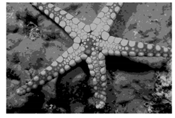 | 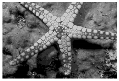 |  | 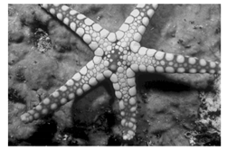 |
 |  |  |  | |
| Image 2 | 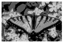 | 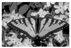 | 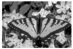 | 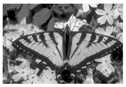 |
 |  |  |  | |
| Image 3 | 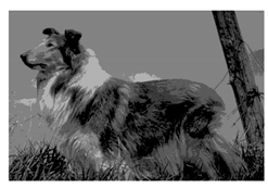 | 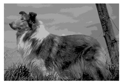 | 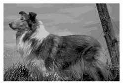 |  |
 |  |  |  | |
| Image 4 | 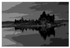 | 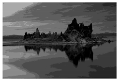 | 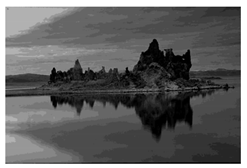 | 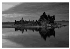 |
 |  |  |  | |
| Image 5 | 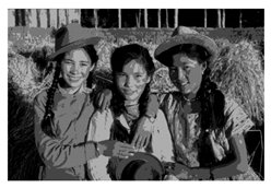 | 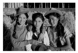 | 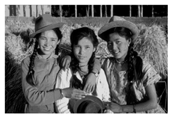 | 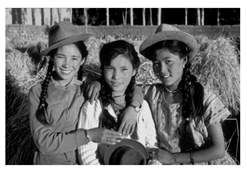 |
 |  |  |  | |
| Image 6 |  |  |  |  |
 |  |  |  | |
| Image 7 | 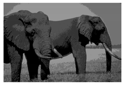 |  |  |  |
 |  |  |  | |
| Image 8 | 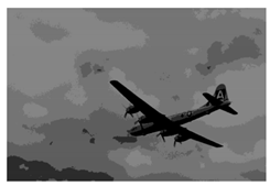 |  |  |  |
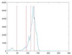 | 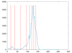 | 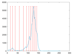 | 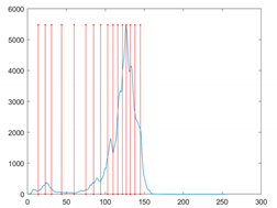 |
Table A3.
The best fitness values obtained by algorithms over all images.
Table A3.
The best fitness values obtained by algorithms over all images.
| Image | nTh | MROA | ROA | RSA | AOA | AO | SSA | SCA | GWO | ||||||||
|---|---|---|---|---|---|---|---|---|---|---|---|---|---|---|---|---|---|
| Mean | Std | Mean | Std | Mean | Std | Mean | Std | Mean | Std | Mean | Std | Mean | Std | Mean | Std | ||
| Image 1 | 4 | 0.7841 | 0 | 0.7841 | 0 | 1.0771 | 0.1565 | 1.1233 | 0.1872 | 0.7841 | 0 | 0.7841 | 0 | 0.8220 | 0.0821 | 0.7841 | 0 |
| 8 | 0.2429 | 0 | 0.2429 | 0 | 0.4622 | 0.0690 | 0.4836 | 0.0737 | 0.2429 | 0 | 0.2430 | 0.0001 | 0.3723 | 0.0476 | 0.2429 | 0 | |
| 12 | 0.1207 | 0.0037 | 0.1213 | 0.0050 | 0.2567 | 0.0372 | 0.2878 | 0.0553 | 0.1222 | 0.0064 | 0.1282 | 0.0081 | 0.2268 | 0.0364 | 0.1337 | 0.0144 | |
| 16 | 0.0713 | 0.0016 | 0.0744 | 0.0049 | 0.1760 | 0.0227 | 0.1784 | 0.0269 | 0.0731 | 0.0048 | 0.0841 | 0.0097 | 0.1659 | 0.0239 | 0.0814 | 0.0096 | |
| Image 2 | 4 | 0.6216 | 0 | 0.6216 | 0 | 0.7838 | 0.0836 | 0.8572 | 0.0885 | 0.6216 | 0 | 0.6216 | 0 | 0.6389 | 0.0084 | 0.6216 | 0 |
| 8 | 0.2052 | 0.0107 | 0.2075 | 0.0149 | 0.3799 | 0.0578 | 0.3868 | 0.0520 | 0.2054 | 0.0107 | 0.2081 | 0.0121 | 0.3064 | 0.0381 | 0.2091 | 0.0179 | |
| 12 | 0.1006 | 0.0063 | 0.0988 | 0.0033 | 0.2058 | 0.0266 | 0.2152 | 0.0350 | 0.1019 | 0.0085 | 0.1060 | 0.0078 | 0.1970 | 0.0185 | 0.1118 | 0.0116 | |
| 16 | 0.0586 | 0.0021 | 0.0622 | 0.0052 | 0.1476 | 0.0207 | 0.1499 | 0.0249 | 0.0640 | 0.0076 | 0.0666 | 0.0042 | 0.1340 | 0.0155 | 0.0736 | 0.0085 | |
| Image 3 | 4 | 0.5146 | 0 | 0.5146 | 0 | 0.6802 | 0.0779 | 0.7292 | 0.1052 | 0.5146 | 0 | 0.5146 | 0 | 0.5276 | 0.0070 | 0.5146 | 0 |
| 8 | 0.1609 | 0 | 0.1678 | 0.0157 | 0.3159 | 0.0545 | 0.3688 | 0.0522 | 0.1625 | 0.0076 | 0.1676 | 0.0142 | 0.2528 | 0.0470 | 0.1679 | 0.0157 | |
| 12 | 0.0788 | 0.0037 | 0.0798 | 0.0065 | 0.1866 | 0.0346 | 0.2186 | 0.0367 | 0.0806 | 0.0068 | 0.0927 | 0.0109 | 0.1659 | 0.0225 | 0.0894 | 0.0084 | |
| 16 | 0.0462 | 0.0015 | 0.0481 | 0.0064 | 0.1322 | 0.0158 | 0.1439 | 0.0267 | 0.0490 | 0.0047 | 0.0631 | 0.0093 | 0.1207 | 0.0167 | 0.0585 | 0.0050 | |
| Image 4 | 4 | 0.7421 | 0 | 0.7421 | 0 | 1.0030 | 0.1326 | 1.1431 | 0.1646 | 0.7421 | 0 | 0.7421 | 0 | 0.7580 | 0.0104 | 0.7421 | 0 |
| 8 | 0.2332 | 0 | 0.2332 | 0 | 0.4483 | 0.0561 | 0.5239 | 0.1076 | 0.2332 | 0.0001 | 0.2568 | 0.0360 | 0.3632 | 0.0557 | 0.2352 | 0.0104 | |
| 12 | 0.1179 | 0.0002 | 0.1180 | 0.0003 | 0.2714 | 0.0429 | 0.3157 | 0.0489 | 0.1191 | 0.0034 | 0.1517 | 0.0171 | 0.2348 | 0.0329 | 0.1243 | 0.0081 | |
| 16 | 0.0699 | 0.0004 | 0.0707 | 0.0022 | 0.1846 | 0.0293 | 0.2172 | 0.0389 | 0.0711 | 0.0020 | 0.1022 | 0.0096 | 0.1754 | 0.0244 | 0.0795 | 0.0057 | |
| Image 5 | 4 | 1.1119 | 0 | 1.1119 | 0 | 1.3808 | 0.1714 | 1.5084 | 0.2439 | 1.1119 | 0 | 1.1119 | 0 | 1.1324 | 0.0128 | 1.1119 | 0 |
| 8 | 0.3530 | 0.0003 | 0.3529 | 0.0002 | 0.5602 | 0.0859 | 0.6133 | 0.0756 | 0.3533 | 0.0004 | 0.3539 | 0.0004 | 0.4862 | 0.0550 | 0.3563 | 0.0158 | |
| 12 | 0.1639 | 0.0001 | 0.1648 | 0.0051 | 0.3297 | 0.0348 | 0.3819 | 0.0345 | 0.1647 | 0.0009 | 0.1811 | 0.0134 | 0.3013 | 0.0356 | 0.1708 | 0.0110 | |
| 16 | 0.0974 | 0.0002 | 0.0977 | 0.0013 | 0.2304 | 0.0352 | 0.2394 | 0.0347 | 0.0987 | 0.0013 | 0.1145 | 0.0087 | 0.2093 | 0.0256 | 0.1074 | 0.0076 | |
| Image 6 | 4 | 0.3155 | 0 | 0.3155 | 0 | 0.4261 | 0.0831 | 0.4697 | 0.0487 | 0.3155 | 0 | 0.3155 | 0 | 0.3284 | 0.0063 | 0.3155 | 0 |
| 8 | 0.1135 | 0 | 0.1145 | 0.0054 | 0.1980 | 0.0208 | 0.2238 | 0.0360 | 0.1167 | 0.0090 | 0.1167 | 0.0093 | 0.1701 | 0.0154 | 0.1136 | 0.0001 | |
| 12 | 0.0583 | 0.0001 | 0.0616 | 0.0054 | 0.1283 | 0.0190 | 0.1345 | 0.0212 | 0.0613 | 0.0038 | 0.0646 | 0.0045 | 0.1175 | 0.0154 | 0.0657 | 0.0055 | |
| 16 | 0.0353 | 0.0003 | 0.0363 | 0.0023 | 0.0911 | 0.0121 | 0.0919 | 0.0131 | 0.0387 | 0.0033 | 0.0418 | 0.0028 | 0.0838 | 0.0102 | 0.0426 | 0.0040 | |
| Image 7 | 4 | 0.4359 | 0 | 0.4359 | 0 | 0.7059 | 0.1129 | 0.7571 | 0.1361 | 0.4359 | 0 | 0.4359 | 0 | 0.4796 | 0.0709 | 0.4359 | 0 |
| 8 | 0.1500 | 0.0065 | 0.1560 | 0.0146 | 0.3189 | 0.0433 | 0.3656 | 0.0734 | 0.1536 | 0.0124 | 0.1600 | 0.0169 | 0.2452 | 0.0381 | 0.1550 | 0.0135 | |
| 12 | 0.0731 | 0.0021 | 0.0797 | 0.0088 | 0.2030 | 0.0325 | 0.2301 | 0.0403 | 0.0741 | 0.0034 | 0.0910 | 0.0077 | 0.1661 | 0.0262 | 0.0833 | 0.0083 | |
| 16 | 0.0435 | 0.0022 | 0.0458 | 0.0039 | 0.1344 | 0.0215 | 0.1487 | 0.0265 | 0.0476 | 0.0069 | 0.0712 | 0.0104 | 0.1244 | 0.0221 | 0.0552 | 0.0059 | |
| Image 8 | 4 | 0.2223 | 0 | 0.2223 | 0 | 0.3345 | 0.0525 | 0.3855 | 0.0672 | 0.2223 | 0 | 0.2223 | 0 | 0.2471 | 0.0318 | 0.2223 | 0 |
| 8 | 0.0773 | 0.0015 | 0.0776 | 0.0016 | 0.1744 | 0.0327 | 0.1959 | 0.0372 | 0.0832 | 0.0072 | 0.1008 | 0.0181 | 0.1431 | 0.0253 | 0.0802 | 0.0098 | |
| 12 | 0.0390 | 0.0013 | 0.0395 | 0.0026 | 0.1121 | 0.0204 | 0.1243 | 0.0181 | 0.0470 | 0.0059 | 0.0591 | 0.0092 | 0.1001 | 0.0151 | 0.0433 | 0.0039 | |
| 16 | 0.0238 | 0.0005 | 0.0241 | 0.0012 | 0.0782 | 0.0136 | 0.0921 | 0.0197 | 0.0306 | 0.0037 | 0.0395 | 0.0060 | 0.0721 | 0.0133 | 0.0300 | 0.0039 | |
Table A4.
The PSNR values obtained by algorithms over all images.
Table A4.
The PSNR values obtained by algorithms over all images.
| Image | nTh | MROA | ROA | RSA | AOA | AO | SSA | SCA | GWO | ||||||||
|---|---|---|---|---|---|---|---|---|---|---|---|---|---|---|---|---|---|
| Mean | Std | Mean | Std | Mean | Std | Mean | Std | Mean | Std | Mean | Std | Mean | Std | Mean | Std | ||
| Image 1 | 4 | 19.3376 | 0 | 19.3376 | 0 | 18.3018 | 0.5249 | 18.1087 | 0.7026 | 19.3376 | 0 | 19.3376 | 0 | 19.2121 | 0.3509 | 19.3376 | 0 |
| 8 | 24.1491 | 0.0004 | 24.1163 | 0.1022 | 21.7778 | 0.7749 | 21.7991 | 0.7920 | 24.1475 | 0.0117 | 24.1281 | 0.0254 | 22.7241 | 0.6679 | 24.1208 | 0.0330 | |
| 12 | 27.1246 | 0.0506 | 27.1175 | 0.1278 | 24.5001 | 0.8100 | 24.2200 | 0.9564 | 27.0969 | 0.1278 | 27.0828 | 0.2336 | 25.0032 | 0.8174 | 26.9968 | 0.2814 | |
| 16 | 29.3117 | 0.3068 | 29.1876 | 0.1377 | 26.1545 | 0.7347 | 26.2696 | 0.8709 | 29.1290 | 0.1958 | 28.9716 | 0.4423 | 26.4606 | 0.8718 | 29.2671 | 0.4458 | |
| Image 2 | 4 | 18.0038 | 0 | 18.0038 | 0 | 17.3395 | 1.0346 | 16.6057 | 0.8798 | 18.0038 | 0 | 18.0038 | 0 | 17.8871 | 0.4044 | 18.0038 | 0 |
| 8 | 22.9234 | 0.2940 | 22.9831 | 0.2279 | 21.4067 | 0.9250 | 20.7784 | 1.4500 | 22.9835 | 0.1557 | 22.9421 | 0.2441 | 21.9460 | 1.0323 | 23.0198 | 0 | |
| 12 | 26.2492 | 0.8132 | 25.9659 | 0.0706 | 24.1938 | 0.9844 | 24.3899 | 1.0967 | 25.9085 | 0.2792 | 26.1072 | 0.5823 | 24.5498 | 0.9768 | 25.9665 | 0.1556 | |
| 16 | 28.6702 | 0.9003 | 28.5102 | 0.4960 | 26.0587 | 1.0591 | 25.9470 | 1.5180 | 28.0976 | 0.5281 | 28.5808 | 0.9061 | 26.1646 | 1.1019 | 28.2240 | 0.3534 | |
| Image 3 | 4 | 19.2818 | 0 | 19.2818 | 0 | 19.6628 | 1.0716 | 18.3815 | 1.3124 | 19.2818 | 0 | 19.2818 | 0 | 19.3864 | 0.4334 | 19.2818 | 0 |
| 8 | 25.0831 | 0.1982 | 25.1037 | 0.1279 | 23.1708 | 0.9900 | 22.1617 | 1.5444 | 25.0772 | 0.1405 | 25.0645 | 0.2753 | 23.8852 | 1.1119 | 25.0825 | 0.0498 | |
| 12 | 28.3161 | 0.3359 | 28.3135 | 0.1234 | 25.9299 | 1.0497 | 25.0463 | 1.2403 | 28.2351 | 0.2469 | 27.9632 | 0.6398 | 26.0484 | 1.0511 | 28.2085 | 0.1756 | |
| 16 | 30.7671 | 0.5883 | 30.4644 | 0.3260 | 27.5699 | 0.8206 | 26.6435 | 1.4561 | 30.3897 | 0.2585 | 30.0481 | 0.7364 | 27.6447 | 1.0729 | 30.3287 | 0.2183 | |
| Image 4 | 4 | 21.5871 | 0 | 21.5871 | 0 | 20.0717 | 0.6269 | 19.6025 | 0.7700 | 21.5871 | 0 | 21.5873 | 0.0015 | 21.4809 | 0.1121 | 21.5871 | 0 |
| 8 | 26.5589 | 0.0069 | 26.5589 | 0.0069 | 23.5589 | 0.5653 | 23.0839 | 0.9430 | 26.5571 | 0.0112 | 26.1229 | 0.6104 | 24.6063 | 0.6936 | 26.5122 | 0.1869 | |
| 12 | 29.6429 | 0.0275 | 29.6386 | 0.0264 | 25.6695 | 0.7268 | 25.4587 | 0.7456 | 29.5274 | 0.1877 | 28.6563 | 0.4896 | 26.5354 | 0.6833 | 29.3460 | 0.2953 | |
| 16 | 31.8382 | 0.0452 | 31.8289 | 0.0953 | 27.2667 | 0.6992 | 27.1155 | 0.9276 | 31.8484 | 0.1858 | 30.5278 | 0.4131 | 27.9195 | 0.7135 | 31.3087 | 0.3760 | |
| Image 5 | 4 | 19.2461 | 0 | 19.2461 | 0 | 17.9538 | 0.6767 | 18.1794 | 0.7934 | 19.2461 | 0 | 19.2461 | 0 | 19.1712 | 0.1436 | 19.2461 | 0 |
| 8 | 23.9514 | 0.0931 | 23.8599 | 0.0533 | 21.8629 | 0.8876 | 21.8907 | 0.6947 | 23.9489 | 0.1324 | 24.1104 | 0.1092 | 22.7269 | 0.4555 | 23.8973 | 0.1859 | |
| 12 | 27.2929 | 0.0189 | 27.2513 | 0.1417 | 24.0802 | 0.6301 | 24.2450 | 0.6203 | 27.1837 | 0.1124 | 27.3553 | 0.1605 | 24.6915 | 0.5420 | 27.0084 | 0.2825 | |
| 16 | 29.4540 | 0.0650 | 29.4478 | 0.0520 | 25.5730 | 0.7455 | 25.9613 | 0.8057 | 29.3635 | 0.1642 | 29.4927 | 0.2483 | 26.2597 | 0.7296 | 29.0170 | 0.3157 | |
| Image 6 | 4 | 21.3607 | 0 | 21.3607 | 0 | 18.1814 | 1.8732 | 19.2881 | 1.6304 | 21.3607 | 0 | 21.3607 | 0 | 21.0657 | 0.5319 | 21.3607 | 0 |
| 8 | 26.7272 | 0.0939 | 26.6653 | 0.1881 | 22.9715 | 1.3210 | 22.9515 | 1.4407 | 26.5535 | 0.3486 | 26.6476 | 0.3186 | 24.7693 | 1.0491 | 26.6911 | 0.0932 | |
| 12 | 30.1561 | 0.0928 | 30.0108 | 0.3028 | 26.1309 | 1.2163 | 26.2053 | 1.4103 | 29.9128 | 0.3887 | 29.8247 | 0.3918 | 26.3476 | 1.2102 | 29.7359 | 0.4487 | |
| 16 | 32.7456 | 0.1698 | 32.7002 | 0.2186 | 27.7064 | 1.4008 | 28.2815 | 1.1492 | 32.2348 | 0.6961 | 31.8480 | 0.4028 | 28.3961 | 1.0373 | 31.8606 | 0.5641 | |
| Image 7 | 4 | 20.6291 | 0 | 20.6291 | 0 | 19.7123 | 0.7668 | 19.4405 | 1.1533 | 20.6291 | 0 | 20.6291 | 0 | 20.4534 | 0.4593 | 20.6291 | 0 |
| 8 | 24.9744 | 0.3290 | 25.0648 | 0.4643 | 23.7591 | 0.7303 | 22.7988 | 1.4098 | 24.9277 | 0.1978 | 24.7888 | 0.5062 | 23.6155 | 0.8901 | 24.9333 | 0.1963 | |
| 12 | 27.8778 | 0.7934 | 27.6887 | 0.6917 | 26.0448 | 0.9770 | 24.7738 | 1.4939 | 27.3320 | 0.3696 | 26.9412 | 0.8687 | 25.9186 | 1.1009 | 27.5552 | 0.7761 | |
| 16 | 30.1065 | 1.0516 | 29.8779 | 1.4726 | 27.9510 | 0.8191 | 26.6208 | 1.7484 | 29.0573 | 0.8782 | 28.7837 | 1.3487 | 27.5947 | 1.4798 | 29.8787 | 1.1793 | |
| Image 8 | 4 | 25.3640 | 0 | 25.3628 | 0.0069 | 22.7034 | 1.2188 | 21.2011 | 1.6455 | 25.3640 | 0 | 25.3640 | 0 | 24.4553 | 1.0689 | 25.3640 | 0 |
| 8 | 30.4785 | 0.1435 | 30.4755 | 0.1480 | 26.0074 | 1.3326 | 25.8519 | 1.0730 | 30.1259 | 0.5866 | 29.0871 | 0.9423 | 27.2603 | 1.1301 | 30.2703 | 0.5812 | |
| 12 | 34.1924 | 0.2804 | 34.1184 | 0.3478 | 28.3594 | 1.1360 | 28.3050 | 0.9239 | 32.9863 | 0.8048 | 32.0325 | 0.8260 | 28.8706 | 1.1758 | 33.4289 | 0.5617 | |
| 16 | 36.7245 | 0.3031 | 36.6173 | 0.4843 | 29.8648 | 1.1453 | 29.6225 | 1.3039 | 35.1034 | 0.6833 | 33.8346 | 0.8438 | 30.8730 | 1.1133 | 35.2055 | 0.7466 | |
Table A5.
The SSIM values obtained by algorithms over all images.
Table A5.
The SSIM values obtained by algorithms over all images.
| Image | nTh | MROA | ROA | RSA | AOA | AO | SSA | SCA | GWO | ||||||||
|---|---|---|---|---|---|---|---|---|---|---|---|---|---|---|---|---|---|
| Mean | Std | Mean | Std | Mean | Std | Mean | Std | Mean | Std | Mean | Std | Mean | Std | Mean | Std | ||
| Image 1 | 4 | 0.6506 | 0 | 0.6506 | 0 | 0.6475 | 0.0198 | 0.5962 | 0.0333 | 0.6506 | 0 | 0.6506 | 0 | 0.6448 | 0.0145 | 0.6506 | 0 |
| 8 | 0.8141 | 0.0072 | 0.8125 | 0 | 0.7867 | 0.0311 | 0.7421 | 0.0349 | 0.8124 | 0.0002 | 0.8114 | 0.0016 | 0.7801 | 0.0225 | 0.8115 | 0.0014 | |
| 12 | 0.8863 | 0.0091 | 0.8810 | 0.0091 | 0.8542 | 0.0238 | 0.8221 | 0.0352 | 0.8792 | 0.0047 | 0.8711 | 0.0114 | 0.8453 | 0.0260 | 0.8858 | 0.0126 | |
| 16 | 0.9179 | 0.0105 | 0.9118 | 0.0033 | 0.8946 | 0.0135 | 0.8652 | 0.0364 | 0.9098 | 0.0033 | 0.9050 | 0.0127 | 0.8871 | 0.0221 | 0.9238 | 0.0125 | |
| Image 2 | 4 | 0.6249 | 0 | 0.6249 | 0 | 0.6777 | 0.0320 | 0.6010 | 0.0581 | 0.6249 | 0 | 0.6249 | 0 | 0.6270 | 0.0209 | 0.6249 | 0 |
| 8 | 0.7948 | 0.0104 | 0.7969 | 0.0069 | 0.7958 | 0.0298 | 0.7489 | 0.0580 | 0.7966 | 0.0038 | 0.7951 | 0.0082 | 0.7848 | 0.0367 | 0.7975 | 0 | |
| 12 | 0.8737 | 0.0191 | 0.8678 | 0.0014 | 0.8442 | 0.0335 | 0.8400 | 0.0345 | 0.8659 | 0.0064 | 0.8704 | 0.0142 | 0.8464 | 0.0284 | 0.8678 | 0.0028 | |
| 16 | 0.9134 | 0.0141 | 0.9115 | 0.0075 | 0.8797 | 0.0213 | 0.8703 | 0.0324 | 0.9054 | 0.0087 | 0.9118 | 0.0144 | 0.8774 | 0.0254 | 0.9074 | 0.0056 | |
| Image 3 | 4 | 0.7280 | 0 | 0.7280 | 0 | 0.7700 | 0.0276 | 0.6831 | 0.0606 | 0.7280 | 0 | 0.7280 | 0 | 0.7174 | 0.0146 | 0.7280 | 0 |
| 8 | 0.8498 | 0.0025 | 0.8514 | 0.0069 | 0.8473 | 0.0283 | 0.7856 | 0.0494 | 0.8491 | 0.0021 | 0.8497 | 0.0061 | 0.8347 | 0.0320 | 0.8488 | 0.0011 | |
| 12 | 0.9061 | 0.0052 | 0.9065 | 0.0022 | 0.8819 | 0.0118 | 0.8518 | 0.0309 | 0.9054 | 0.0040 | 0.9000 | 0.0112 | 0.8724 | 0.0225 | 0.9054 | 0.0023 | |
| 16 | 0.9369 | 0.0065 | 0.9345 | 0.0036 | 0.9019 | 0.0138 | 0.8795 | 0.0302 | 0.9332 | 0.0033 | 0.9267 | 0.0087 | 0.8961 | 0.0223 | 0.9324 | 0.0030 | |
| Image 4 | 4 | 0.7478 | 0 | 0.7478 | 0 | 0.7678 | 0.0146 | 0.7199 | 0.0327 | 0.7478 | 0 | 0.7478 | 0 | 0.7469 | 0.0085 | 0.7478 | 0 |
| 8 | 0.8399 | 0.0006 | 0.8399 | 0.0006 | 0.8327 | 0.0099 | 0.7845 | 0.0229 | 0.8391 | 0.0005 | 0.8359 | 0.0071 | 0.8253 | 0.0110 | 0.8398 | 0.0008 | |
| 12 | 0.8914 | 0.0010 | 0.8911 | 0.0011 | 0.8604 | 0.0092 | 0.8314 | 0.0193 | 0.8906 | 0.0019 | 0.8704 | 0.0085 | 0.8581 | 0.0131 | 0.8911 | 0.0031 | |
| 16 | 0.9232 | 0.0010 | 0.9230 | 0.0019 | 0.8839 | 0.0094 | 0.8633 | 0.0136 | 0.9228 | 0.0019 | 0.8977 | 0.0072 | 0.8823 | 0.0100 | 0.9215 | 0.0034 | |
| Image 5 | 4 | 0.6850 | 0 | 0.6850 | 0 | 0.6788 | 0.0139 | 0.6360 | 0.0297 | 0.6850 | 0 | 0.6850 | 0 | 0.6827 | 0.0040 | 0.6850 | 0 |
| 8 | 0.8219 | 0.0012 | 0.8215 | 0.0007 | 0.8076 | 0.0246 | 0.7678 | 0.0288 | 0.8208 | 0.0017 | 0.8190 | 0.0012 | 0.8136 | 0.0191 | 0.8207 | 0.0032 | |
| 12 | 0.8945 | 0.0002 | 0.8871 | 0.0009 | 0.8720 | 0.0219 | 0.8253 | 0.0289 | 0.8865 | 0.0010 | 0.8794 | 0.0069 | 0.8632 | 0.0219 | 0.8908 | 0.0058 | |
| 16 | 0.9401 | 0.0091 | 0.9204 | 0.0019 | 0.9024 | 0.0164 | 0.8723 | 0.0236 | 0.9203 | 0.0014 | 0.9105 | 0.0061 | 0.9045 | 0.0177 | 0.9387 | 0.0123 | |
| Image 6 | 4 | 0.8741 | 0 | 0.8741 | 0 | 0.8858 | 0.0110 | 0.8568 | 0.0364 | 0.8741 | 0 | 0.8741 | 0 | 0.8754 | 0.0063 | 0.8741 | 0 |
| 8 | 0.8866 | 0.0015 | 0.8859 | 0.0021 | 0.9173 | 0.0155 | 0.8801 | 0.0282 | 0.8843 | 0.0047 | 0.8862 | 0.0041 | 0.9028 | 0.0212 | 0.8863 | 0.0013 | |
| 12 | 0.9206 | 0.0014 | 0.9200 | 0.0027 | 0.9159 | 0.0230 | 0.8994 | 0.0225 | 0.9190 | 0.0033 | 0.9174 | 0.0043 | 0.9036 | 0.0230 | 0.9204 | 0.0038 | |
| 16 | 0.9405 | 0.0018 | 0.9401 | 0.0019 | 0.9154 | 0.0197 | 0.9169 | 0.0138 | 0.9376 | 0.0055 | 0.9342 | 0.0036 | 0.9190 | 0.0123 | 0.9359 | 0.0043 | |
| Image 7 | 4 | 0.6896 | 0 | 0.6896 | 0 | 0.7146 | 0.0281 | 0.6598 | 0.0524 | 0.6896 | 0 | 0.6896 | 0 | 0.6848 | 0.0117 | 0.6896 | 0 |
| 8 | 0.8237 | 0.0125 | 0.8261 | 0.0170 | 0.8352 | 0.0235 | 0.7800 | 0.0562 | 0.8214 | 0.0077 | 0.8172 | 0.0155 | 0.7918 | 0.0293 | 0.8220 | 0.0078 | |
| 12 | 0.8891 | 0.0166 | 0.8849 | 0.0143 | 0.8729 | 0.0212 | 0.8261 | 0.0456 | 0.8771 | 0.0074 | 0.8664 | 0.0189 | 0.8507 | 0.0330 | 0.8815 | 0.0155 | |
| 16 | 0.9214 | 0.0149 | 0.9172 | 0.0200 | 0.9022 | 0.0141 | 0.8602 | 0.0403 | 0.9064 | 0.0134 | 0.9004 | 0.0232 | 0.8803 | 0.0321 | 0.9185 | 0.0173 | |
| Image 8 | 4 | 0.8567 | 0 | 0.8566 | 0.0005 | 0.8657 | 0.0227 | 0.8352 | 0.0382 | 0.8567 | 0 | 0.8567 | 0 | 0.8468 | 0.0112 | 0.8567 | 0 |
| 8 | 0.9113 | 0.0032 | 0.9107 | 0.0035 | 0.8871 | 0.0145 | 0.8719 | 0.0166 | 0.9065 | 0.0049 | 0.8973 | 0.0078 | 0.8857 | 0.0106 | 0.9096 | 0.0054 | |
| 12 | 0.9400 | 0.0023 | 0.9395 | 0.0026 | 0.9053 | 0.0136 | 0.8936 | 0.0101 | 0.9303 | 0.0063 | 0.9225 | 0.0068 | 0.8991 | 0.0137 | 0.9349 | 0.0042 | |
| 16 | 0.9571 | 0.0022 | 0.9566 | 0.0031 | 0.9153 | 0.0113 | 0.9096 | 0.0108 | 0.9458 | 0.0048 | 0.9369 | 0.0060 | 0.9193 | 0.0109 | 0.9482 | 0.0049 | |
Table A6.
The FSIM values obtained by algorithms over all images.
Table A6.
The FSIM values obtained by algorithms over all images.
| Image | nTh | MROA | ROA | RSA | AOA | AO | SSA | SCA | GWO | ||||||||
|---|---|---|---|---|---|---|---|---|---|---|---|---|---|---|---|---|---|
| Mean | Std | Mean | Std | Mean | Std | Mean | Std | Mean | Std | Mean | Std | Mean | Std | Mean | Std | ||
| Image 1 | 4 | 0.7693 | 0 | 0.7693 | 0 | 0.7333 | 0.0173 | 0.7247 | 0.0219 | 0.7693 | 0 | 0.7693 | 0 | 0.7630 | 0.0105 | 0.7693 | 0 |
| 8 | 0.8902 | 0 | 0.8895 | 0.0025 | 0.8342 | 0.0184 | 0.8259 | 0.0184 | 0.8902 | 0.0001 | 0.8902 | 0.0003 | 0.8527 | 0.0135 | 0.8901 | 0.0002 | |
| 12 | 0.9348 | 0.0004 | 0.9347 | 0.0014 | 0.8847 | 0.0128 | 0.8736 | 0.0202 | 0.9346 | 0.0018 | 0.9335 | 0.0025 | 0.8943 | 0.0134 | 0.9329 | 0.0034 | |
| 16 | 0.9548 | 0.0025 | 0.9538 | 0.0005 | 0.9129 | 0.0099 | 0.9104 | 0.0127 | 0.9540 | 0.0016 | 0.9535 | 0.0031 | 0.9175 | 0.0112 | 0.9544 | 0.0037 | |
| Image 2 | 4 | 0.7666 | 0 | 0.7666 | 0 | 0.7740 | 0.0137 | 0.7618 | 0.0158 | 0.7666 | 0 | 0.7666 | 0 | 0.7705 | 0.0078 | 0.7666 | 0 |
| 8 | 0.8704 | 0.0026 | 0.8701 | 0.0036 | 0.8410 | 0.0124 | 0.8303 | 0.0209 | 0.8702 | 0.0026 | 0.8704 | 0.0026 | 0.8498 | 0.0154 | 0.8707 | 0 | |
| 12 | 0.9211 | 0.0064 | 0.9202 | 0.0010 | 0.8858 | 0.0133 | 0.8840 | 0.0151 | 0.9190 | 0.0037 | 0.9205 | 0.0041 | 0.8885 | 0.0137 | 0.9201 | 0.0026 | |
| 16 | 0.9474 | 0.0058 | 0.9461 | 0.0031 | 0.9086 | 0.0135 | 0.9065 | 0.0182 | 0.9432 | 0.0046 | 0.9469 | 0.0054 | 0.9118 | 0.0139 | 0.9449 | 0.0023 | |
| Image 3 | 4 | 0.7903 | 0 | 0.7903 | 0 | 0.7933 | 0.0779 | 0.7529 | 0.0278 | 0.7903 | 0 | 0.7903 | 0 | 0.7860 | 0.0049 | 0.7903 | 0 |
| 8 | 0.8894 | 0.0029 | 0.8901 | 0.0033 | 0.8692 | 0.0545 | 0.8310 | 0.0276 | 0.8891 | 0.0021 | 0.8891 | 0.0047 | 0.8690 | 0.0223 | 0.8891 | 0.0008 | |
| 12 | 0.9314 | 0.0043 | 0.9327 | 0.0016 | 0.9034 | 0.0346 | 0.8821 | 0.0216 | 0.9317 | 0.0032 | 0.9293 | 0.0076 | 0.9012 | 0.0156 | 0.9315 | 0.0018 | |
| 16 | 0.9554 | 0.0057 | 0.9513 | 0.0028 | 0.9226 | 0.0158 | 0.9076 | 0.0225 | 0.9509 | 0.0025 | 0.9500 | 0.0063 | 0.9221 | 0.0153 | 0.9501 | 0.0021 | |
| Image 4 | 4 | 0.7982 | 0 | 0.7982 | 0 | 0.8032 | 0.0075 | 0.7842 | 0.0131 | 0.7982 | 0 | 0.7982 | 0.0002 | 0.7991 | 0.0044 | 0.7982 | 0 |
| 8 | 0.8639 | 0.0001 | 0.8639 | 0.0001 | 0.8371 | 0.0082 | 0.8223 | 0.0146 | 0.8640 | 0.0003 | 0.8598 | 0.0066 | 0.8431 | 0.0089 | 0.8636 | 0.0016 | |
| 12 | 0.9055 | 0.0004 | 0.9054 | 0.0005 | 0.8630 | 0.0108 | 0.8541 | 0.0100 | 0.9034 | 0.0032 | 0.8902 | 0.0062 | 0.8664 | 0.0085 | 0.9012 | 0.0037 | |
| 16 | 0.9277 | 0.0007 | 0.9274 | 0.0010 | 0.8809 | 0.0087 | 0.8765 | 0.0121 | 0.9274 | 0.0021 | 0.9129 | 0.0055 | 0.8838 | 0.0092 | 0.9253 | 0.0032 | |
| Image 5 | 4 | 0.8264 | 0 | 0.8264 | 0 | 0.7921 | 0.0185 | 0.7861 | 0.0235 | 0.8264 | 0 | 0.8264 | 0 | 0.8239 | 0.0033 | 0.8264 | 0 |
| 8 | 0.9063 | 0.0024 | 0.9057 | 0.0013 | 0.8750 | 0.0133 | 0.8686 | 0.0157 | 0.9061 | 0.0035 | 0.9116 | 0.0024 | 0.8862 | 0.0089 | 0.9073 | 0.0036 | |
| 12 | 0.9474 | 0.0002 | 0.9471 | 0.0011 | 0.9101 | 0.0085 | 0.9043 | 0.0100 | 0.9468 | 0.0008 | 0.9474 | 0.0020 | 0.9156 | 0.0074 | 0.9457 | 0.0021 | |
| 16 | 0.9649 | 0.0005 | 0.9642 | 0.0009 | 0.9270 | 0.0093 | 0.9258 | 0.0081 | 0.9646 | 0.0009 | 0.9642 | 0.0020 | 0.9362 | 0.0065 | 0.9647 | 0.0024 | |
| Image 6 | 4 | 0.8669 | 0 | 0.8669 | 0 | 0.8631 | 0.0066 | 0.8496 | 0.0135 | 0.8669 | 0 | 0.8669 | 0 | 0.8659 | 0.0021 | 0.8669 | 0 |
| 8 | 0.8903 | 0.0007 | 0.8900 | 0.0009 | 0.8924 | 0.0071 | 0.8749 | 0.0140 | 0.8897 | 0.0021 | 0.8903 | 0.0018 | 0.8905 | 0.0115 | 0.8903 | 0.0006 | |
| 12 | 0.9223 | 0.0008 | 0.9205 | 0.0034 | 0.9039 | 0.0128 | 0.8945 | 0.0118 | 0.9190 | 0.0039 | 0.9183 | 0.0038 | 0.9010 | 0.0116 | 0.9178 | 0.0037 | |
| 16 | 0.9397 | 0.0010 | 0.9396 | 0.0012 | 0.9127 | 0.0118 | 0.9114 | 0.0092 | 0.9379 | 0.0043 | 0.9350 | 0.0026 | 0.9151 | 0.0085 | 0.9356 | 0.0037 | |
| Image 7 | 4 | 0.8223 | 0 | 0.8223 | 0 | 0.8036 | 0.0113 | 0.7793 | 0.0250 | 0.8223 | 0 | 0.8223 | 0 | 0.8116 | 0.0076 | 0.8223 | 0 |
| 8 | 0.8889 | 0.0036 | 0.8902 | 0.0051 | 0.8719 | 0.0123 | 0.8483 | 0.0167 | 0.8885 | 0.0015 | 0.8844 | 0.0048 | 0.8685 | 0.0121 | 0.8885 | 0.0021 | |
| 12 | 0.9226 | 0.0077 | 0.9214 | 0.0064 | 0.9005 | 0.0127 | 0.8805 | 0.0176 | 0.9176 | 0.0022 | 0.9154 | 0.0085 | 0.8898 | 0.0115 | 0.9208 | 0.0093 | |
| 16 | 0.9424 | 0.0090 | 0.9421 | 0.0117 | 0.9227 | 0.0094 | 0.9051 | 0.0150 | 0.9343 | 0.0038 | 0.9354 | 0.0111 | 0.9141 | 0.0151 | 0.9411 | 0.0084 | |
| Image 8 | 4 | 0.8587 | 0 | 0.8586 | 0.0005 | 0.8623 | 0.0089 | 0.8552 | 0.0120 | 0.8587 | 0 | 0.8587 | 0 | 0.8548 | 0.0060 | 0.8587 | 0 |
| 8 | 0.8889 | 0.0043 | 0.8879 | 0.0046 | 0.8710 | 0.0096 | 0.8671 | 0.0116 | 0.8835 | 0.0050 | 0.8761 | 0.0058 | 0.8684 | 0.0065 | 0.8871 | 0.0058 | |
| 12 | 0.9199 | 0.0039 | 0.9188 | 0.0039 | 0.8812 | 0.0103 | 0.8774 | 0.0093 | 0.9077 | 0.0078 | 0.8998 | 0.0075 | 0.8779 | 0.0103 | 0.9120 | 0.0059 | |
| 16 | 0.9446 | 0.0034 | 0.9437 | 0.0052 | 0.8900 | 0.0089 | 0.8879 | 0.0098 | 0.9281 | 0.0074 | 0.9159 | 0.0077 | 0.8950 | 0.0103 | 0.9293 | 0.0077 | |
Table A7.
The p-values obtained by algorithms over all images.
Table A7.
The p-values obtained by algorithms over all images.
| Image | nTh | ROA | RSA | AOA | AO | SSA | SCA | GWO |
|---|---|---|---|---|---|---|---|---|
| Image 1 | 4 | 6.54 × 10−01 | 3.15 × 10⁻¹² | 3.15 × 10⁻¹² | 4.59 × 10−02 | 4.59 × 10−01 | 3.15 × 10⁻¹² | 2.89 × 10−01 |
| 8 | 3.34 × 10−01 | 1.21 × 10⁻¹² | 1.21 × 10⁻¹² | 4.19 × 10−02 | 4.38 × 10⁻¹² | 1.21 × 10⁻¹² | 2.89 × 10−05 | |
| 12 | 7.19 × 10−01 | 7.87 × 10⁻¹² | 7.87 × 10⁻¹² | 2.25 × 10−08 | 7.87 × 10⁻¹² | 7.87 × 10⁻¹² | 1.19 × 10⁻¹¹ | |
| 16 | 2.24 × 10−03 | 2.92 × 10⁻¹¹ | 2.92 × 10⁻¹¹ | 8.70 × 10⁻¹¹ | 2.92 × 10⁻¹¹ | 2.92 × 10⁻¹¹ | 8.70 × 10⁻¹¹ | |
| Image 2 | 4 | NaN | 1.21 × 10⁻¹² | 1.21 × 10⁻¹² | NaN | NaN | 1.21 × 10⁻¹² | NaN |
| 8 | 1.76 × 10−01 | 1.25 × 10⁻¹¹ | 1.25 × 10⁻¹¹ | 2.69 × 10−01 | 1.30 × 10−06 | 1.25 × 10⁻¹¹ | 4.69 × 10−02 | |
| 12 | 5.08 × 10−03 | 2.37 × 10⁻¹¹ | 2.37 × 10⁻¹¹ | 1.07 × 10−06 | 7.87 × 10⁻¹¹ | 2.37 × 10⁻¹¹ | 2.88 × 10−09 | |
| 16 | 1.80 × 10−02 | 3.01 × 10⁻¹¹ | 3.01 × 10⁻¹¹ | 5.48 × 10⁻¹¹ | 3.01 × 10⁻¹¹ | 3.01 × 10⁻¹¹ | 3.01 × 10⁻¹¹ | |
| Image 3 | 4 | NaN | 1.21 × 10⁻¹² | 1.21 × 10⁻¹² | NaN | NaN | 1.21 × 10⁻¹² | NaN |
| 8 | 1.10 × 10−01 | 4.10 × 10⁻¹² | 4.10 × 10⁻¹² | 3.99 × 10−01 | 5.00 × 10−08 | 4.10 × 10⁻¹² | 7.38 × 10−07 | |
| 12 | 2.30 × 10−01 | 2.83 × 10⁻¹¹ | 2.83 × 10⁻¹¹ | 2.42 × 10−05 | 9.33 × 10⁻¹¹ | 2.83 × 10⁻¹¹ | 7.65 × 10⁻¹¹ | |
| 16 | 5.45 × 10−06 | 3.01 × 10⁻¹¹ | 3.01 × 10⁻¹¹ | 2.15 × 10⁻¹⁰ | 3.01 × 10⁻¹¹ | 3.01 × 10⁻¹¹ | 3.01 × 10⁻¹¹ | |
| Image 4 | 4 | NaN | 1.21 × 10⁻¹² | 1.21 × 10⁻¹² | NaN | NaN | 1.21 × 10⁻¹² | NaN |
| 8 | 1.98 × 10−02 | 1.04 × 10⁻¹¹ | 1.04 × 10⁻¹¹ | 8.90 × 10−01 | 1.05 × 10−07 | 1.04 × 10⁻¹¹ | 4.98 × 10−02 | |
| 12 | 4.65 × 10−02 | 9.04 × 10⁻¹² | 9.04 × 10⁻¹² | 2.10 × 10−05 | 9.04 × 10⁻¹² | 9.04 × 10⁻¹² | 9.04 × 10⁻¹² | |
| 16 | 8.92 × 10−03 | 2.95 × 10⁻¹¹ | 2.95 × 10⁻¹¹ | 2.62 × 10−09 | 3.26 × 10⁻¹¹ | 2.95 × 10⁻¹¹ | 2.95 × 10⁻¹¹ | |
| Image 5 | 4 | NaN | 1.21 × 10⁻¹² | 1.21 × 10⁻¹² | NaN | NaN | 1.21 × 10⁻¹² | NaN |
| 8 | 4.98 × 10−01 | 1.76 × 10⁻¹¹ | 1.76 × 10⁻¹¹ | 2.68 × 10−02 | 4.15 × 10−09 | 1.76 × 10⁻¹¹ | 2.37 × 10−02 | |
| 12 | 2.13 × 10−01 | 2.20 × 10⁻¹¹ | 2.20 × 10⁻¹¹ | 1.51 × 10−03 | 6.01 × 10⁻¹¹ | 2.20 × 10⁻¹¹ | 1.94 × 10−08 | |
| 16 | 5.72 × 10−02 | 2.86 × 10⁻¹¹ | 2.86 × 10⁻¹¹ | 4.00 × 10−09 | 2.86 × 10⁻¹¹ | 2.86 × 10⁻¹¹ | 7.73 × 10⁻¹⁰ | |
| Image 6 | 4 | NaN | 1.21 × 10⁻¹² | 1.21 × 10⁻¹² | NaN | NaN | 1.21 × 10⁻¹² | NaN |
| 8 | 3.38 × 10−02 | 2.82 × 10⁻¹¹ | 2.82 × 10⁻¹¹ | 3.03 × 10−04 | 6.93 × 10−01 | 2.82 × 10⁻¹¹ | 2.15 × 10−01 | |
| 12 | 1.79 × 10−02 | 3.00 × 10⁻¹¹ | 3.00 × 10⁻¹¹ | 9.02 × 10−08 | 3.00 × 10⁻¹¹ | 3.00 × 10⁻¹¹ | 3.98 × 10−09 | |
| 16 | 3.33 × 10−01 | 3.02 × 10⁻¹¹ | 3.02 × 10⁻¹¹ | 3.01 × 10−07 | 3.02 × 10⁻¹¹ | 3.02 × 10⁻¹¹ | 1.56 × 10−08 | |
| Image 7 | 4 | NaN | 1.21 × 10⁻¹² | 1.21 × 10⁻¹² | NaN | NaN | 1.21 × 10⁻¹² | NaN |
| 8 | 4.36 × 10−02 | 8.87 × 10⁻¹² | 8.87 × 10⁻¹² | 4.91 × 10−02 | 9.87 × 10−08 | 8.87 × 10⁻¹² | 1.42 × 10−04 | |
| 12 | 4.56 × 10−02 | 2.22 × 10⁻¹¹ | 2.22 × 10⁻¹¹ | 5.89 × 10−04 | 1.22 × 10⁻¹⁰ | 2.22 × 10⁻¹¹ | 3.05 × 10⁻¹⁰ | |
| 16 | 4.49 × 10−02 | 2.96 × 10⁻¹¹ | 2.96 × 10⁻¹¹ | 2.06 × 10−08 | 2.96 × 10⁻¹¹ | 2.96 × 10⁻¹¹ | 4.00 × 10⁻¹¹ | |
| Image 8 | 4 | 7.08 × 10−01 | 5.14 × 10⁻¹² | 5.14 × 10⁻¹² | 1.78 × 10−02 | 1.05 × 10−01 | 5.14 × 10⁻¹² | 4.59 × 10−01 |
| 8 | 5.63 × 10−01 | 2.94 × 10⁻¹¹ | 2.94 × 10⁻¹¹ | 6.64 × 10−02 | 7.78 × 10−08 | 2.94 × 10⁻¹¹ | 2.90 × 10−02 | |
| 12 | 2.51 × 10−02 | 3.01 × 10⁻¹¹ | 3.01 × 10⁻¹¹ | 8.88 × 10⁻¹⁰ | 3.01 × 10⁻¹¹ | 3.01 × 10⁻¹¹ | 3.33 × 10⁻¹¹ | |
| 16 | 3.87 × 10−01 | 3.02 × 10⁻¹¹ | 3.02 × 10⁻¹¹ | 8.15 × 10⁻¹¹ | 3.02 × 10⁻¹¹ | 3.02 × 10⁻¹¹ | 3.02 × 10⁻¹¹ |
Table A8.
The CPU time for the MROA and comparison algorithms.
Table A8.
The CPU time for the MROA and comparison algorithms.
| Image | nTh | MROA | ROA | RSA | AOA | AO | SSA | SCA | GWO |
|---|---|---|---|---|---|---|---|---|---|
| Image 1 | 4 | 1.8379 | 1.2774 | 0.7673 | 0.5887 | 1.1524 | 0.6932 | 0.6409 | 0.6846 |
| 8 | 1.9090 | 1.2922 | 0.7895 | 0.5915 | 1.1807 | 0.7011 | 0.5479 | 0.6018 | |
| 12 | 2.1367 | 1.4243 | 0.9846 | 0.6058 | 1.1919 | 0.7098 | 0.6852 | 0.6668 | |
| 16 | 2.2943 | 1.5839 | 1.0903 | 0.6425 | 1.2171 | 0.7163 | 0.6630 | 0.7468 | |
| Image 2 | 4 | 1.8884 | 1.3400 | 0.7926 | 0.6556 | 1.1092 | 0.6537 | 0.6434 | 0.6246 |
| 8 | 1.9155 | 1.2544 | 0.7368 | 0.6092 | 1.0052 | 0.6236 | 0.5540 | 0.6029 | |
| 12 | 2.1956 | 1.4925 | 0.8888 | 0.6844 | 1.1197 | 0.6210 | 0.5861 | 0.6386 | |
| 16 | 2.3795 | 1.5326 | 1.0408 | 0.6702 | 1.2512 | 0.6586 | 0.6819 | 0.6626 | |
| Image 3 | 4 | 1.8430 | 1.3069 | 0.7711 | 0.5950 | 1.1376 | 0.6922 | 0.6540 | 0.6255 |
| 8 | 1.9125 | 1.3168 | 0.7436 | 0.5538 | 0.9963 | 0.6033 | 0.5804 | 0.6135 | |
| 12 | 2.1190 | 1.5218 | 0.8806 | 0.5997 | 1.1744 | 0.6486 | 0.5827 | 0.6043 | |
| 16 | 2.2936 | 1.5352 | 1.0334 | 0.7055 | 1.2035 | 0.7296 | 0.6459 | 0.6791 | |
| Image 4 | 4 | 1.8630 | 1.3688 | 0.7957 | 0.6722 | 1.1309 | 0.6726 | 0.6945 | 0.6642 |
| 8 | 1.9396 | 1.3100 | 0.7478 | 0.5843 | 1.0390 | 0.5498 | 0.5735 | 0.6127 | |
| 12 | 2.1422 | 1.4025 | 0.9128 | 0.6430 | 1.0708 | 0.6095 | 0.5939 | 0.6114 | |
| 16 | 2.5628 | 1.5249 | 1.0577 | 0.7174 | 1.1687 | 0.6639 | 0.7192 | 0.6939 | |
| Image 5 | 4 | 1.8642 | 1.3274 | 0.8288 | 0.6242 | 1.1396 | 0.6730 | 0.6344 | 0.6666 |
| 8 | 1.8793 | 1.3911 | 0.7755 | 0.5829 | 1.0591 | 0.5451 | 0.5688 | 0.5600 | |
| 12 | 2.1781 | 1.4372 | 0.9106 | 0.5894 | 1.0738 | 0.5873 | 0.5887 | 0.5966 | |
| 16 | 2.2633 | 1.5203 | 1.0575 | 0.6301 | 1.1780 | 0.6432 | 0.7161 | 0.6593 | |
| Image 6 | 4 | 1.8582 | 1.4131 | 0.8380 | 0.6121 | 1.1232 | 0.6806 | 0.6570 | 0.6517 |
| 8 | 2.0519 | 1.2756 | 0.7370 | 0.5501 | 1.0023 | 0.6240 | 0.5383 | 0.5697 | |
| 12 | 2.1120 | 1.4508 | 0.8868 | 0.5959 | 1.1090 | 0.6999 | 0.5964 | 0.6241 | |
| 16 | 2.3020 | 1.5646 | 1.0270 | 0.6463 | 1.2760 | 0.7085 | 0.6445 | 0.6864 | |
| Image 7 | 4 | 1.8690 | 1.3777 | 0.7855 | 0.6232 | 1.1237 | 0.6944 | 0.6329 | 0.6491 |
| 8 | 1.9270 | 1.3281 | 0.7436 | 0.5353 | 0.9974 | 0.5933 | 0.5332 | 0.5566 | |
| 12 | 2.1831 | 1.3844 | 0.8867 | 0.5838 | 1.0896 | 0.6509 | 0.5947 | 0.6173 | |
| 16 | 2.3213 | 1.5032 | 1.1525 | 0.6419 | 1.1959 | 0.7408 | 0.6577 | 0.6742 | |
| Image 8 | 4 | 1.8611 | 1.3340 | 0.7880 | 0.6387 | 1.1718 | 0.7102 | 0.6407 | 0.6419 |
| 8 | 1.9048 | 1.3356 | 0.7345 | 0.5370 | 1.0652 | 0.5539 | 0.5455 | 0.5838 | |
| 12 | 2.1167 | 1.3882 | 0.8858 | 0.5777 | 1.1787 | 0.6169 | 0.5821 | 0.6676 | |
| 16 | 2.4502 | 1.5255 | 1.0484 | 0.6479 | 1.2839 | 0.7311 | 0.6500 | 0.6957 |
References
- Bhandari, A.K. A novel beta differential evolution algorithm-based fast multilevel thresholding for color image segmentation. Neural Comput. Appl. 2020, 32, 4583–4613. [Google Scholar] [CrossRef]
- He, L.; Huang, S. An efficient krill herd algorithm for color image multilevel thresholding segmentation problem. Appl. Soft Comput. 2020, 89, 106063. [Google Scholar] [CrossRef]
- Bhandari, A.K.; Rahul, K. A novel local contrast fusion-based fuzzy model for color image multilevel thresholding using grasshopper optimization. Appl. Soft Comput. 2019, 81, 105515. [Google Scholar] [CrossRef]
- Bhattacharyya, S.; Maulik, U.; Dutta, P. Multilevel image segmentation with adaptive image context based thresholding. Appl. Soft Comput. 2011, 11, 946–962. [Google Scholar] [CrossRef]
- Anitha, J.; Pandian, I.A.; Agnes, S.A. An efficient multilevel color image thresholding based on modified whale optimization algorithm. Expert Syst. Appl. 2021, 178, 115003. [Google Scholar] [CrossRef]
- Lei, B.; Fan, J. Multilevel minimum cross entropy thresholding: A comparative study. Appl. Soft Comput. 2020, 96, 106588. [Google Scholar] [CrossRef]
- Lin, S.; Jia, H.; Abualigah, L.; Altalhi, M. Enhanced slime mould algorithm for multilevel thresholding image segmentation using entropy measures. Entropy 2021, 23, 1700. [Google Scholar] [CrossRef]
- Kotte, S.; Pullakura, R.K.; Injeti, S.K. Optimal multilevel thresholding selection for brain MRI image segmentation based on adaptive wind driven optimization. Measurement 2018, 130, 340–361. [Google Scholar] [CrossRef]
- Houssein, E.H.; Emam, M.M.; Ali, A.A. An efficient multilevel thresholding segmentation method for thermography breast cancer imaging based on improved chimp optimization algorithm. Expert Syst. Appl. 2021, 185, 115651. [Google Scholar] [CrossRef]
- Zhou, Y.; Yang, X.; Ling, Y.; Zhang, J. Meta-heuristic moth swarm algorithm for multilevel thresholding image segmentation. Multimed. Tools Appl. 2018, 77, 23699–23727. [Google Scholar] [CrossRef]
- Jiang, Y.; Yeh, W.; Hao, Z.; Yang, Z. A cooperative honey bee mating algorithm and its application in multi-threshold image segmentation. Inform. Sci. 2016, 369, 171–183. [Google Scholar] [CrossRef]
- Sarkar, S.; Das, S. Multilevel Image Thresholding Based on 2D Histogram and Maximum Tsallis Entropy—A Differential Evolution Approach. IEEE Trans. Image Process 2013, 22, 4788–4797. [Google Scholar] [CrossRef] [PubMed]
- Ahmadi, M.; Kazemi, K.; Aarabi, A.; Niknam, T.; Helfroush, M.S. Image segmentation using multilevel thresholding based on modified bird mating optimization. Multimed. Tools Appl. 2017, 78, 23003–23027. [Google Scholar] [CrossRef]
- Abualigah, L.; Diabat, A.; Sumari, P.; Gandomi, A.H. A novel evolutionary arithmetic optimization algorithm for multilevel thresholding segmentation of COVID-19 CT images. Processes 2021, 9, 1155. [Google Scholar] [CrossRef]
- Chen, H.; Li, W.; Yang, X. A whale optimization algorithm with chaos mechanism based on quasi-opposition for global optimization problems. Expert Syst. Appl. 2020, 158, 113612. [Google Scholar] [CrossRef]
- Rao, R.V.; Vakharia, D.P. Teaching-learning-based optimization: A novel method for constrained mechanical design optimization problems. Comput. Aided Des. 2011, 43, 303–315. [Google Scholar] [CrossRef]
- Wang, S.; Liu, Q.; Liu, Y.; Jia, H.; Abualigah, L.; Zheng, R.; Wu, D. A hybrid SSA and SMA with mutation opposition-based learning for constrained engineering problems. Comput. Intell. Neurosci. 2021, 2021, 6379469. [Google Scholar] [CrossRef]
- Dinkar, S.K.; Deep, K.; Mirjalili, S.; Thapliyal, S. Opposition-based Laplacian Equilibrium Optimizer with application in image segmentation using multilevel thresholding. Expert Syst. Appl. 2021, 174, 114766. [Google Scholar] [CrossRef]
- Zheng, R.; Jia, H.; Abualigah, L.; Liu, Q.; Wang, S. Deep ensemble of slime mold algorithm and arithmetic optimization algorithm for global optimization. Processes 2021, 9, 1774. [Google Scholar] [CrossRef]
- Wang, S.; Jia, H.; Liu, Q.; Zheng, R. An improved hybrid aquila optimizer and harris hawks optimization for global optimization. Math. Biosci. Eng. 2021, 18, 7076–7109. [Google Scholar] [CrossRef]
- Houssein, E.H.; Mahdy, M.A.; Blondin, M.J.; Shebl, D.; Mohamed, W.M. Hybrid slime mould algorithm with adaptive guided differential evolution algorithm for combinatorial and global optimization problems. Expert Syst. Appl. 2021, 174, 114689. [Google Scholar] [CrossRef]
- Zheng, R.; Jia, H.; Abualigah, L.; Liu, Q.; Wang, S. An improved arithmetic optimization algorithm with forced switching mechanism for global optimization problems. Math. Biosci. Eng. 2021, 19, 473–512. [Google Scholar] [CrossRef] [PubMed]
- Wang, S.; Jia, H.; Abualigah, L.; Liu, Q.; Zheng, R. An improved hybrid aquila optimizer and harris hawks algorithm for solving industrial engineering optimization problems. Processes 2021, 9, 1551. [Google Scholar] [CrossRef]
- Li, Y.; Zhao, Y.; Liu, J. Dynamic sine cosine algorithm for large-scale global optimization problems. Expert Syst. Appl. 2021, 177, 114950. [Google Scholar] [CrossRef]
- Zhang, Z.; Ding, S.; Jia, W. A hybrid optimization algorithm based on cuckoo search and differential evolution for solving constrained engineering problems. Eng. Appl. Artif. Intel. 2019, 85, 254–268. [Google Scholar] [CrossRef]
- Khare, A.; Rangnekar, S. A review of particle swarm optimization and its applications in solar photovoltaic system. Appl. Soft Comput. 2013, 13, 2997–3006. [Google Scholar] [CrossRef]
- Mirjalili, S.; Mirjalili, S.M.; Lewis, A. Grey wolf optimizer. Adv. Eng. Softw. 2014, 69, 46–61. [Google Scholar] [CrossRef] [Green Version]
- Li, S.; Chen, H.; Wang, M.; Heidari, A.A.; Mirjalili, S. Slime mould algorithm: A new method for stochastic optimization. Future Gener. Comput. Syst. 2020, 111, 300–323. [Google Scholar] [CrossRef]
- Mirjalili, S.; Lewis, A. The whale optimization algorithm. Adv. Eng. Softw. 2016, 95, 51–67. [Google Scholar] [CrossRef]
- Abdel-Basset, M.; Hessin, A.N.; Abdel-Fatah, L. A comprehensive study of cuckoo-inspired algorithms. Neural Comput. Appl. 2018, 29, 345–361. [Google Scholar] [CrossRef]
- Mirjalili, S.; Gandomi, A.H.; Mirjalili, S.Z.; Saremi, S.; Faris, H.; Mirjalili, S.M. Salp swarm algorithm: A bio-inspired optimizer for engineering design problems. Adv. Eng. Softw. 2017, 114, 163–191. [Google Scholar] [CrossRef]
- Dorigo, M.; Birattari, M.; Stutzle, T. Ant colony optimization. IEEE Comput. Intell. Mag. 2006, 1, 28–39. [Google Scholar] [CrossRef]
- Heidari, A.A.; Mirjalili, S.; Faris, H.; Aljarah, I.; Mafarja, M.; Chen, H. Harris hawks optimization: Algorithm and applications. Future Gener. Comput. Syst. 2019, 97, 849–872. [Google Scholar] [CrossRef]
- Mirjalili, S. Moth-flame optimization algorithm: A novel nature-inspired heuristic paradigm. Knowl. Based Syst. 2015, 89, 228–249. [Google Scholar] [CrossRef]
- Abualigah, L.; Yousri, D.; Abd, E.M.; Ewees, A.A. Aquila optimizer: A novel meta-heuristic optimization algorithm. Comput. Ind. Eng. 2021, 157, 107250. [Google Scholar] [CrossRef]
- Katoch, S.; Chauhan, S.S.; Kumar, V. A review on genetic algorithm: Past, present, and future. Multimed. Tools Appl. 2021, 80, 8091–8126. [Google Scholar] [CrossRef]
- Rakshit, P.; Konar, A.; Das, S. Noisy evolutionary optimization algorithms—A comprehensive survey. Swarm Evol. Comput. 2017, 33, 18–45. [Google Scholar] [CrossRef]
- Slowik, A.; Kwasnicka, H. Evolutionary algorithms and their applications to engineering problems. Neural Comput. Appl. 2020, 32, 12363–12379. [Google Scholar] [CrossRef] [Green Version]
- Nguyen, S.; Mei, Y.; Zhang, M. Genetic programming for production scheduling: A survey with a unified framework. Complex Intell. Syst. 2017, 3, 41–66. [Google Scholar] [CrossRef] [Green Version]
- Simon, D. Biogeography-based optimization. IEEE Trans. Evol. Comput. 2008, 12, 702–713. [Google Scholar] [CrossRef] [Green Version]
- Hansen, N.; Ostermeier, A. Completely Derandomized Self-Adaptation in Evolution Strategies. Evol. Comput. 2001, 9, 159–195. [Google Scholar] [CrossRef]
- Kirkpatrick, S.; Gelatt, C.D.; Vecchi, M.P. Optimization by simulated annealing. Science 1983, 220, 671–680. [Google Scholar] [CrossRef]
- Rashedi, E.; Nezamabadi-pour, H.; Saryazdi, S. GSA: A gravitational search algorithm. Inform. Sci. 2009, 179, 2232–2248. [Google Scholar] [CrossRef]
- Ahmadianfar, I.; Haddad, O.B.; Chu, X. Gradient-based optimizer: A new metaheuristic optimization algorithm. Inform. Sci. 2020, 540, 131–159. [Google Scholar] [CrossRef]
- Mirjalili, S. SCA: A sine cosine algorithm for solving optimization problems. Knowl. Based Syst. 2016, 96, 120–133. [Google Scholar] [CrossRef]
- Tanyildizi, E.; Demir, G. Golden sine algorithm: A novel math-inspired algorithm. Golden sine algorithm: A novel math-inspired algorithm. Adv. Electr. Comput. Eng. 2017, 17, 71–78. [Google Scholar] [CrossRef]
- Abualigah, L.; Diabat, A.; Mirjalili, S.; Elaziz, A.E.; Gandomi, A.H. The arithmetic optimization algorithm. Comput. Methods Appl. Mech. Eng. 2021, 376, 113609. [Google Scholar] [CrossRef]
- Neggaz, N.; Houssein, E.H.; Hussain, K. An efficient henry gas solubility optimization for feature selection. Expert Syst. Appl. 2020, 152, 113364. [Google Scholar] [CrossRef]
- Sun, P.; Liu, H.; Zhang, Y.; Meng, Q.; Tu, L.; Zhao, J. An improved atom search optimization with dynamic opposite learning and heterogeneous comprehensive learning. Appl. Soft Comput. 2021, 103, 107140. [Google Scholar] [CrossRef]
- Liu, Y.; Tian, P. A multi-start central force optimization for global optimization. Appl. Soft Comput. 2015, 27, 92–98. [Google Scholar] [CrossRef]
- Mirjalili, S.; Mirjalili, S.M.; Hatamlou, A. Multi-verse optimizer: A nature-inspired algorithm for global optimization. Neural. Comput. Appl. 2015, 27, 495–513. [Google Scholar] [CrossRef]
- Jia, H.; Peng, X.; Lang, C. Remora optimization algorithm. Expert Syst. Appl. 2021, 185, 115665. [Google Scholar] [CrossRef]
- Zheng, R.; Jia, H.; Abualigah, L.; Wang, S.; Wu, D. An improved remora optimization algorithm with autonomous foraging mechanism for global optimization problems. Math. Biosci. Eng. 2022, 19, 3994–4037. [Google Scholar] [CrossRef]
- Wolpert, D.H.; Macready, W.G. No free lunch theorems for optimization. IEEE Trans. Evol. Comput. 1997, 1, 67–82. [Google Scholar] [CrossRef] [Green Version]
- Jia, H.; Lang, C.; Oliva, D.; Song, W.; Peng, X. Dynamic harris hawks optimization with mutation mechanism for satellite image segmentation. Remote Sens. 2019, 11, 1421. [Google Scholar] [CrossRef] [Green Version]
- Ewees, A.A.; Abualigah, L.; Yousri, D.; Sahlol, A.T.; Al-qaness, A.A.; Alshathri, S.; Elaziz, M.A. Modified artificial ecosystem-based optimization for multilevel thresholding image segmentation. Mathematics 2021, 9, 2363. [Google Scholar] [CrossRef]
- Houssein, E.H.; Hussain, K.; Abualigah, L.; Elaziz, M.A.; Alomoush, W.; Dhiman, G.; Djenouri, Y.; Cuevas, E. An improved opposition-based marine predators algorithms for global optimization and multilevel thresholding image segmentation. Knowl.-Based Syst. 2021, 229, 107348. [Google Scholar] [CrossRef]
- Su, H.; Zhao, D.; Yu, F.; Heidari, A.A.; Zhang, Y.; Chen, H.; Li, C.; Pan, J.; Quan, S. Horizontal and vertical search artificial bee colony for image segmentation of COVID-19 X-ray images. Comput. Biol. Med. 2021, 142, 105181. [Google Scholar] [CrossRef]
- Liu, L.; Zhao, D.; Yu, F.; Heidari, A.A.; Ru, J.; Chen, H.; Mafarja, M.; Turabieh, H.; Pan, Z. Performance optimization of differential evolution with slime mould algorithm for multilevel breast cancer image segmentation. Comput. Biol. Med. 2021, 138, 104910. [Google Scholar] [CrossRef]
- Li, Y.; Bai, X.; Jiao, L.; Xue, Y. Partitioned-cooperative quantum-behaved particle swarm optimization based on multilevel thresholding applied to medical image segmentation. Appl. Soft Comput. 2017, 56, 345–356. [Google Scholar] [CrossRef]
- Sun, K.; Jia, H.; Li, Y.; Jiang, Z. Hybrid improved slime mould algorithm with adaptive β hill climbing for numerical optimization. J. Intell. Fuzzy Syst. 2021, 40, 1667–1679. [Google Scholar] [CrossRef]
- Faramarzi, A.; Heidarinejad, M.; Mirjalili, S.; Gandomi, A.H. Marine predators algorithm: A nature-inspired metaheuristic. Expert Syst. Appl. 2020, 152, 113377. [Google Scholar] [CrossRef]
- Tizhoosh, H.R. Opposition-based learning: A new scheme for machine intelligence. In Proceedings of the Computational Intelligence for Modelling, Control & Automation, Vienna, Austria, 28–30 November 2005. [Google Scholar]
- Chauhan, S.; Vashishtha, G.; Kumar, A. A symbiosis of arithmetic optimizer with slime mould algorithm for improving global optimization and conventional design problem. J. Supercomput. 2022, 78, 6234–6274. [Google Scholar] [CrossRef]
- Kullback, S. Information Theory and Statistics; Dover: New York, NY, USA, 1968. [Google Scholar]
- Oliva, D.; Hinojosa, S.; Cuevas, E.; Pajares, G.; Avalos, O.; Galvez, J. Cross entropy based thresholding for magnetic resonance brain images using Crow Search Algorithm. Expert Syst. Appl. 2017, 79, 164–180. [Google Scholar] [CrossRef]
- Esparza, E.R.; Calzada, L.A.Z.; Oliva, D.; Heidari, A.A.; Zaldivar, D.; Cisneros, M.P.; Foong, L.K. An efficient harris hawks-inspired image segmentation method. Expert Syst. Appl. 2020, 155, 113428. [Google Scholar] [CrossRef]
- Gill, H.S.; Khehra, B.S.; Singh, A.; Kaur, L. Teaching-learning-based optimization algorithm to minimize cross entropy for Selecting multilevel threshold values. Egypt. Inform. J. 2019, 20, 11–25. [Google Scholar] [CrossRef]
- Abualigah, L.; Elaziz, M.A.; Sumari, P.; Geem, Z.; Gandomi, A.H. Reptile search algorithm (RSA): A nature-inspired meta-heuristic optimizer. Expert Syst. Appl. 2022, 191, 116158. [Google Scholar] [CrossRef]
- Houssein, E.H.; Neggaz, N.; Hosney, M.E.; Mohamed, W.M.; Hassaballah, M. Enhanced Harris hawks optimization with genetic operators for selection chemical descriptors and compounds activities. Neural Comput. Appl. 2021, 33, 13601–13618. [Google Scholar] [CrossRef]
- Bao, X.; Jia, H.; Lang, C. A Novel Hybrid Harris Hawks Optimization for Color Image Multilevel Thresholding Segmentation. IEEE Access 2019, 7, 76529–76546. [Google Scholar] [CrossRef]
- Sara, U.; Akter, M.; Uddin, M.S. Image quality assessment through FSIM, SSIM, MSE and PSNR—A comparative study. J. Comput. Commun. 2019, 7, 8–18. [Google Scholar] [CrossRef] [Green Version]
- Wang, Z.; Bovik, A.C.; Sheikh, H.R.; Simoncelli, E.P. Image quality assessment: From error visibility to structural similarity. IEEE Trans. Image Process. 2004, 13, 600–612. [Google Scholar] [CrossRef] [PubMed] [Green Version]
- Jia, H.; Ma, J.; Song, W. Multilevel Thresholding Segmentation for Color Image Using Modified Moth-Flame Optimization. IEEE Access 2019, 7, 44097–44134. [Google Scholar] [CrossRef]
- Xing, Z. An improved emperor penguin optimization based multilevel thresholding for color image segmentation. Knowl. Based Syst. 2020, 194, 105570. [Google Scholar] [CrossRef]
Publisher’s Note: MDPI stays neutral with regard to jurisdictional claims in published maps and institutional affiliations. |
© 2022 by the authors. Licensee MDPI, Basel, Switzerland. This article is an open access article distributed under the terms and conditions of the Creative Commons Attribution (CC BY) license (https://creativecommons.org/licenses/by/4.0/).