Modeling Spheres in Some Paranormed Sequence Spaces

Abstract

We introduce a new sequence space $h_A\left(p\right)$, which is not normable, in general, and show that it is a paranormed space. Here, A and p denote an infinite matrix and a sequence of positive numbers. In the special case, when A is a diagonal matrix with a sequence d of positive terms on its diagonal and $p=(1,1,\dots )$, then $h_A\left(p\right)$ reduces to the generalized Hahn space $h_d$. We applied our own software to visualize the shapes of parts of spheres in three-dimensional space endowed with the relative paranorm of $h_A\left(p\right)$, when A is an upper triangle. For this, we developed a parametric representation of these spheres and solved the visibility and contour (silhouette) problems. Finally, we demonstrate the effects of the change of the entries of the upper triangle A and the terms of the sequence p on the shape of the spheres.

1. Introduction

Modeling and visualization are widely used in teaching and research as useful tools for better understanding mathematical concepts and results. They are also frequently applied in natural and engineering sciences.

Here, we used our own software to visualize the geometry of linear metric spaces that have recently been used and studied in functional analysis and operator theory. This goal was achieved by visualizing spheres in the metric of the studied spaces.

We introduce a new sequence space $h_A\left(p\right)$, prove that it is a linear metric space with respect to its natural total paranorm, and solve the visibility and contour (silhouette) problems for the visualization of spheres or their parts in three-dimensional space endowed with the relative paranorm of $h_A\left(p\right)$.

Finally, we demonstrate the influence of the change of the entries of the matrix A and the terms of the sequence p on the shapes of the spheres in the relative metric of $h_A\left(p\right)$ in three-dimensional space.

All the figures in this paper were created by our own software for the visualization of mathematical objects and concepts, in particular of curves and surfaces in three-dimensional space. The development of our software started in 1993 for the purpose of helping students better understand the topics of classical differential geometry. The original software is explained in detail in the book [1]. One major interest in differential geometry concerns the properties of curves, surfaces, and curves on surfaces such as geodesic and asymptotic lines and lines of curvature. This is the reason for our approach to represent surfaces exclusively by families of curves on them. Since we do not approximate surfaces, the accuracy of the curves on them can be as precise as desirable, within the limits of the representation of real numbers and the used methods of computation. This results in smooth-looking curves even in very large-sized graphics.

Over the years, it turned out that our software is also useful in the visualization of our scientific results. We applied it for the graphical representations of our results, for instance, in topology [2], crystallography [3], paranormed spaces [4], and Hahn spaces [5]. In this paper, we used it for illustrating some results in functional analysis.

In this paper, we represent surfaces, which are spheres in various metrics, by two families of curves, in particular by parameter lines in green and blue. This gives the spheres a natural look. The well-known shape of the spheres in Euclidean metrics is a special case of the shapes of the spheres we represent. The other surfaces appear as distortions of Euclidean spheres.

We used central projection in our software with the free choice of all parameters. The center of projection is given in spherical coordinates, because they give a better idea of its position.

The visibility of points was checked analytically immediately after the computation of their coordinates. A point on surface is visible (with respect to the surface) if it is not hidden by any other point of the same surface that lies on the projection ray. Therefore, we have to compute the intersection of the projection ray with the surface. In particular, we found values $u_1$ and $u_2$ of the parameters in the parametric representation of the surface and the value of t in the parametric representation of the projection ray. The computation of these parameters is given in Section 4.

Since we used only curves to represent surfaces, their representations appear unfinished without their silhouettes. This involves the partial derivatives of the parametric representation of the surfaces. The necessary computations are described in Section 4. In the figures in this paper, the silhouettes are represented by thick black curves.

2. A New Class of Paranormed Sequence Spaces

Here, we introduce a new class of sequence spaces and discuss some topological properties of the spaces.

We use the standard notations $\omega$ for the set of all complex sequences $x={\left(x_k\right)}_{k=1}^{\infty }$ and $c_0$ and $\varphi$ for the sets of all sequences in $\omega$ that converge to zero and that terminate in zeros, respectively. Let $e={\left(e_k\right)}_{k=1}^{\infty }$ and $e^{\left(n\right)}={(e_k^{\left(n\right)})}_{k=1}^{\infty }$ for $n\in \mathbb{N}$ be the sequences with $e_k=1$ for all k and $e_n^{\left(n\right)}=1$ and $e_k^{\left(n\right)}=0$ for $k\ne n$. Furthermore, for every sequence $x={\left(x_k\right)}_{k=1}^{\infty }\in \omega$ and $m\in \mathbb{N}$, let:

$$x^{\left[n\right]}=\sum _{k=1}^n{x}_k{e}^{\left(k\right)}$$

be the so-called n-section of the sequence x.

We recall the concept of a paranorm (see, for instance [6], Definition 4.2.1).

Definition 1.

Let X be a linear space.

A function$g:X\to \mathbb{R}$is called a paranorm, if for all $x,y\in X$:

$g\left(0\right)=0,$	(P.1)
$g\left(x\right)\ge 0,$	(P.2)
$g(-x)=g\left(x\right),$	(P.3)
$g(x+y)\le g\left(x\right)+g\left(y\right)(\mathrm{triangle} \mathrm{inequality})$	(P.4)
$if\left(x_n\right) is a sequence of vectors with \underset{n\to \infty }{lim}g(x_n-x)=0 and \left({\lambda }_n\right)$
$is a sequence of scalars with \underset{n\to \infty }{lim}{\lambda }_n=\lambda , then \underset{n\to \infty }{lim}g({\lambda }_n{x}_n-$	(P.5)
$\lambda x)=0(\mathrm{continuity} \mathrm{of} \mathrm{multiplication} \mathrm{by} \mathrm{scalars}).$

A paranormed space$(X,g)$(or simply X) is a linear space endowed with a paranorm g. A paranorm g is said to be total, if $g\left(x\right)=0$ implies $x=0$.

Remark 1.

If g is a total paranorm for a linear space X, then obviously$d(x,y)=g(x-y)$for all$x,y\in X$defines a metric on X, which is translation invariant. Hence, every totally paranormed space is a linear metric space. The converse statement is also true. The metric of any linear metric space is given by some total paranorm ([6] Theorem 10.4.2).

Remark 2.

It is well known ([6] Theorem 4.4.1) that ω is a complete totally paranormed space with respect$g_{\omega }$defined by:

$$g_{\omega }\left(x\right)=\sum _{k=1}^{\infty }{\displaystyle \frac{1}{2^k}}·{\displaystyle \frac{|x_k|}{1+|x_k|}}(x={\left(x_k\right)}_{k=1}^{\infty }\in \omega ),$$

and:

$$\underset{n\to \infty }{lim}{g}_{\omega }(x^{\left(n\right)})=0 if and only if \underset{n\to \infty }{lim}\left|x_k^{\left(n\right)}\right|=0 for each k,$$

that is convergence in ω and coordinatewise convergence are equivalent.

An $FK$ space X is a subset of $\omega$, which is a complete linear metric space with its metric d stronger than the metric $d_{\omega }$ on X, that is convergence in $(X,d)$ implies coordinatewise convergence ([7] Definition 9.2.1, Remark 9.2.2). If the metric of an $FK$ space X is normable, then X is called a $BK$ space. An $FK$ space $X\supset \varphi$ is said to have $AK$ ([7] Definition 9.2.12), if every sequence $x={\left(x_k\right)}_{k=1}^{\infty }\in X$ has a unique representation $x={lim}_{n\to \infty }{x}^{\left[n\right]}$.

Remark 3.

Many authors include local convexity in the definition of an $FK$ space; we did not, because it was not needed in our studies.

Example 1.

(a) ([7] Example 9.2.12 (b)) The set ω is an$FK$space with$AK$with respect to the metric$d_{\omega }$defined by$d_{\omega }(x,y)=g_{\omega }(x-y)$for all sequences$x={\left(x_k\right)}_{k=1}^{\infty },y={\left(y_k\right)}_{k=1}^{\infty }\in \omega$; (b) ([8,9,10] and [11] Theorem 2) Let$p={\left(p_k\right)}_{k=1}^{\infty }$be a sequence of positive real numbers, and:

$$\ell \left(p\right)=\left\{x\in \omega :\sum _{k=1}^{\infty }{\left|x_k\right|}^{p_k}<\infty \right\} and c_0\left(p\right)=\left\{x\in \omega :\underset{k\to \infty }{lim}{\left|x_k\right|}^{p_k}=0\right\}.$$

In the case where the terms of the sequence p are constant, say$p_k=p$for all k, then the sets$\ell \left(p\right)$and$c_0\left(p\right)$reduce to the classical spaces${\ell }_p$and$c_0$. If the sequence p is bounded and$M={max}_k\{1,p_k\}$, then$\ell \left(p\right)$and$c_0\left(p\right)$are$FK$spaces with$AK$with respect to their natural paranorms$g_{\left(p\right)}$and$g_{0,\left(p\right)}$, respectively, where:

$$g_{\left(p\right)}\left(x\right)={\left(\sum _{k=1}^{\infty }{\left|x_k\right|}^{p_k}\right)}^{1/M}and{g}_{0,\left(p\right)}\left(x\right)=\underset{k}{sup}{\left|x_k\right|}^{p_k/M}.$$

It is easy to see that$\ell \left(p\right)$and$c_0\left(p\right)$are not linear spaces, when the sequence p is not bounded.

Let $A={\left(a_{nk}\right)}_{n,k=1}^{\infty }$ be an infinite matrix of complex entries, $x={\left(x_k\right)}_{k=1}^{\infty }\in \omega$ and $X\subset \omega$. We write $A_n={\left(a_{nk}\right)}_{k=1}^{\infty }$$(n\in \mathbb{N})$ for the sequence in the $n\mathrm{th}$ row of A:

$$A_{n}x=\sum _{k=1}^{\infty }{a}_{nk}{x}_k \mathrm{for} \mathrm{each} n \mathrm{and} Ax={\left(A_{n}x\right)}_{n=1}^{\infty }$$

provided all the series $A_{n}x$ converge. The set:

$$X_A=\{x\in \omega :Ax\in X\}$$

is called the matrix domain of A in X.

The Hahn space h was originally introduced and studied by Hahn in 1922 [12] in connection with the theory of singular integrals, and later generalized to $h_d$ by Goes [13] for sequences $d={\left(d_k\right)}_{k=1}^{\infty }$ of positive reals, where:

$$h_d=\{x\in \omega :\sum _{k=1}^{\infty }{d}_k|\mathsf{\Delta }{x}_k|<\infty \}\cap c_0,$$

and $\mathsf{\Delta }{x}_k=x_k-x_{k+1}$ for all k. In the special cases, where $d_k=k$ or $d_k=1$ for all k, the generalized Hahn space reduces to the original Hahn space h or the classical space $b{v}_0$ (see, for instance [14], Definition 7.3.3), respectively. It was shown in [15], Proposition 2.1, that if the sequence d is increasing and unbounded, then $h_d$ is a $BK$ space with $AK$.

Matrix transformations and bounded and compact operators on the Hahn space have recently been studied in various papers, for instance in [5,15,16,17,18,19,20,21,22,23]. Spectra on the Hahn space were studied in [16,24,25]. A survey of recent results can also be found in [18].

We generalize the definition of the space $h_d$ as follows.

Let $A={\left(a_{nk}\right)}_{n,k=1}^{\infty }$ be a finite matrix with complex entries and ${\left(p_k\right)}_{k=1}^{\infty }$ be a bounded sequence of positive real numbers. We define the set:

$$h_A\left(p\right)={(\ell \left(p\right))}_A\cap c_0\left(p\right).$$

If $A={\left(a_{nk}\right)}_{n,k=1}^{\infty }$ is given by $a_{nn}=d_n$, $a_{n,n+1}=-d_n$ and $a_{nk}=0$ for $k\ne n,n+1$ and $n=1,2,\dots$, then $h_A\left(e\right)=h_d$.

3. The Generalized Paranormed Hahn Space ${\mathit{h}}_{\mathit{A}}\left(\mathit{p}\right)$

Throughout, let ${\left(p_k\right)}_{k=1}^{\infty }$ be a sequence of positive real numbers and $A={\left(a_{nk}\right)}_{n,k=1}^{\infty }$ be an infinite matrix of complex entries. In this section, we show that the space $h_A\left(p\right)$ is a totally paranormed space, if the sequence p is bounded.

The following holds.

Proposition 1.

Let the sequence $p={\left(p_k\right)}_{k=1}^{\infty }$ be bounded and $M=max\{1,{sup}_k{p}_k\}$. Then, $(h_d\left(p\right),g_{A,\left(p\right)})$ is a paranormed space with:

$$g_{A,\left(p\right)}\left(x\right)={\left(\sum _{n=1}^{\infty }{\left|A_{n}x\right|}^{p_n}\right)}^{1/M}(x\in h_A\left(p\right)).$$

Proof. 

Throughout, we write $g=g_{A,\left(p\right)}$ for short:

(i)

First, we show that $Y=h_A\left(p\right)$ is a linear space.

• We write ${\alpha }_k=p_k/M$.

• Let $x,y\in Y$. Then, $x,y\in c_0\left(p\right)$, and so, since ${\alpha }_k\le 1$ for all k,

  $$|x_k+y_k{|}^{{\alpha }_k}\le |x_k{|}^{{\alpha }_k}+{\left|y_k\right|}^{{\alpha }_k}\to 0(k\to \infty );$$

  hence, $x+y\in c_0\left(p\right)$. Applying Minkowski’s inequality, we obtain:

  $$\begin{array}{cc}\hfill {\left(\sum _{n=1}^{\infty }{\left|A_n(x+y)\right|}^{p_n}\right)}^{1/M}& ={\left(\sum _{n=1}^{\infty }{\left({\left|A_{n}x+A_{n}y\right|}^{{\alpha }_n}\right)}^M\right)}^{1/M}\hfill \\ \hfill & \le {\left(\sum _{n=1}^{\infty }{\left|A_{n}x\right|}^{{\alpha }_{n}M}\right)}^{1/M}+{\left(\sum _{n=1}^{\infty }{\left|A_{n}y\right|}^{{\alpha }_{n}M}\right)}^{1/M}\hfill \\ \hfill & ={\left(\sum _{n=1}^{\infty }{\left|A_{n}x\right|}^{p_n}\right)}^{1/M}+{\left(\sum _{n=1}^{\infty }{\left|A_{n}y\right|}^{p_n}\right)}^{1/M}<\infty .\hfill \end{array}$$

  (1)

  Therefore, we proved that Y is closed with respect to addition.

• Now, we assume $x\in Y$ and $\lambda \in \mathbb{C}$. We put $\mathsf{\Lambda }=max\{1,|\lambda {|}^M\}$, and obtained from $x\in c_0\left(p\right)$:

  $${\left|\lambda x_k\right|}^{p_k}\le \mathsf{\Lambda }{\left|x_k\right|}^{p_k}\to 0(k\to \infty )$$

  that $\lambda x\in c_0\left(p\right)$, and also:

  $$\sum _{k=1}^{\infty }{\left|A_n\left(\lambda x\right)\right|}^{p_n}\le \mathsf{\Lambda }\sum _{n=1}^{\infty }{\left|A_{n}x\right|}^{p_n}<\infty ;$$

  hence, $\lambda x\in Y$. This completes Part (i) of the proof;

(ii)

Now, we show that g is a total paranorm on Y.

• Obviously, $g:Y\to \mathbb{R}$ satisfies (P.1), (P.2), and (P.3) and, by (1), also (P.4) in Definition 1.
• To prove (P.5), we assume that $x^{\left(n\right)}={(x_k^{\left(n\right)})}_{k=1}^{\infty }$ is a sequence of elements in Y with ${lim}_{n\to \infty }g(x^{\left(n\right)}-x)=0$ and ${\left({\lambda }_n\right)}_{n=1}^{\infty }$ is a sequence of scalars with ${lim}_{n\to \infty }{\lambda }_n=\lambda$. It follows that:

  $$g\left({\lambda }_n{x}^{\left(n\right)}-\lambda x\right)\le S_{1;n}+S_{2;n}+S_{3;n},$$

  (2)

  where:

  $$S_{1;n}=g\left(({\lambda }_n-\lambda )(x^{\left(n\right)}-x)\right),S_{2;n}=g\left(\lambda (x^{\left(n\right)}-x)\right) \mathrm{and} S_{3;n}=g\left(({\lambda }_n-\lambda )x\right).$$
• First, ${lim}_{n\to \infty }{\lambda }_n=\lambda$ implies $|{\lambda }_n-\lambda |\le 1$ for all sufficiently large n; hence:

  $$0\le S_{1;n}\le g\left(x^{\left(n\right)}-x\right)\to 0(n\to \infty ).$$

  We also have:

  $$0\le S_{2;n}\le \mathsf{\Lambda }g\left(x^{\left(n\right)}-x\right)\to 0(n\to \infty ).$$
• Finally, to show $S_{3;n}\to 0$$(n\to \infty )$, let $\epsilon >0$ be given. Then, there exists $k_0\in \mathbb{N}$ such that:

  $${\left(\sum _{k=k_0+1}^{\infty }{\left|A_{k}x\right|}^{p_k}\right)}^{1/M}<{\displaystyle \frac{\epsilon }{2}}.$$
• Now, we choose $n_0\in \mathbb{N}$ such that:

  $$|{\lambda }_n-\lambda |\le 1 \mathrm{and} \underset{1\le k\le k_0}{max}{|{\lambda }_n-\lambda |}^{p_k}\le {\left({\displaystyle \frac{\epsilon }{2g\left(x\right)+1}}\right)}^M \mathrm{for} \mathrm{all} n\ge n_0.$$
• Since $1/M\le 1$, we obtain for all $n\ge n_0$:

  $$\begin{array}{cc}\hfill S_{3;n}& ={\left(\sum _{k=1}^{\infty }|{\lambda }_n{-\lambda |}^{p_k}{\left|A_{k}x\right|}^{p_k}\right)}^{1/M}\hfill \\ \hfill & \le {\left(\sum _{k=1}^{k_0}|{\lambda }_n{-\lambda |}^{p_k}{\left|A_{k}x\right|}^{p_k}\right)}^{1/M}+{\left(\sum _{k=k_0+1}^{\infty }|{\lambda }_n{-\lambda |}^{p_k}{\left|A_{k}x\right|}^{p_k}\right)}^{1/M}\hfill \\ \hfill & \le {\displaystyle \frac{\epsilon }{2g\left(x\right)+1}}·{\left(\sum _{k=1}^{\infty }{\left|A_{k}x\right|}^{p_k}\right)}^{1/M}+{\left(\sum _{k=k_0+1}^{\infty }{\left|A_{k}x\right|}^{p_k}\right)}^{1/M}\hfill \\ \hfill & <{\displaystyle \frac{\epsilon }{2}}+{\displaystyle \frac{\epsilon }{2}}=\epsilon .\hfill \end{array}$$

  Hence, we also have $S_{3;n}\to 0$$(n\to \infty )$, and consequently, the condition in (P.5) of Definition 1 is satisfied. □

Remark 4.

(a) If the matrix A is such that the map$L_A:\ell \left(p\right)\to h_A\left(p\right)$is one to one, then$g_{A,\left(p\right)}$clearly is total; (b) If the sequence p is not bounded, then$h_A\left(p\right)$need not be a linear space, in general. For instance, if we choose$A=I$, the identity matrix, then$h_I\left(p\right)=\ell \left(p\right)$, and it is well known that$\ell \left(p\right)$is not a linear space when p is unbounded ([26], Example 1.12 (a)).

4. Visibility and Contour

The computations and results of this section were used for the implementation of the methods in our software to create the figures in this paper. For this, we studied the visibility and contour problems for parts $S_r$ of spheres of radius $r>0$ in three-dimensional space ${\mathbb{V}}^3$ with respect to the restriction ${\left.g_{A,\left(p\right)}\right|}_{{\mathbb{V}}^3}$ on ${\mathbb{V}}^3$ of the paranorm $g_{A,\left(p\right)}$, where A is an upper triangle. We recall that an infinite matrix $A={\left(a_{nk}\right)}_{n,k=1}^{\infty }$ is said to be an upper triangle if $a_{nn}\ne 0$ and $a_{nk}=0$ for $k<n$ $(n=0,1,\dots )$. We identify the three-section $z^{\left[3\right]}$ of any sequence $z\in \omega$ with the vector $\overrightarrow{z}=\{z_1,z_2,z_3\}$. Let $A={\left(a_{nk}\right)}_{n,k=1}^3$ be a $(3\times 3)$-matrix, which is an upper triangle, and $\overrightarrow{x}=\{x_1,x_2,x_3\}\in {\mathbb{V}}^3$, then we write, as usual,

$$A_n\overrightarrow{x}=\sum _{k=n}^3{a}_{nk}{x}_k \mathrm{for} n=1,2,3$$

and define the ${\left.g_{A,\left(p\right)}\right|}_{{\mathbb{V}}^3}$ by:

$${\left.g_{A,\left(p\right)}\right|}_{{\mathbb{V}}^3}\left({\left(A{x}^{\left[3\right]}\right)}^{\left[3\right]}\right)={\left(\sum _{n=1}^3{\left|A_n\overrightarrow{x}\right|}^{p_n}\right)}^{1/M},$$

where $M=max\{1,p_1,p_2,p_3\}$ (Figure 1).

Figure 1. Part of a sphere.

We assume that $S_r$ has a parametric representation:

$$\overrightarrow{x}(u_1,u_2)((u_1,u_2)\in R=I_1\times I_2),$$

(3)

where $I_1\subset (-\pi /2,\pi /2)$ and $I_2=(0,2\pi )$.

First, we solved the visibility problem.

We used central projection in ${\mathbb{V}}^3$ and checked the visibility of any point on a given surface analytically. This means we had to compute the intersections of straight lines with the surface S.

We write $g={\left.g_{A,\left(p\right)}\right|}_{{\mathbb{V}}^3}$. Since g is translation invariant by Remark 1, it is sufficient to solve the visibility problem for parts $S_r$ of spheres centered at zero.

We write for $(u_1,u_2)\in R$:

$$s_1=\mathrm{sgn}(sin{u}_1),s_2=\mathrm{sgn}(sin{u}_2),c_2=\mathrm{sgn}(cos{u}_2),$$

$$\left\{\begin{array}{cc}\hfill y_1(u_1,u_2)& =c_2{r}^{M/p_1}{\left(cos{u}_1|cos{u}_2|\right)}^{2/p_1}\hfill \\ \hfill y_2(u_1,u_2)& =s_2{r}^{M/p_2}{\left(cos{u}_1|sin{u}_2|\right)}^{2/p_2}\hfill \\ \hfill y_3(u_1,u_2)& =s_1{r}^{M/p_3}{\left|sin{u}_1\right|}^{2/p_3}.\hfill \end{array}\right\}$$

(4)

Since A is an upper triangle, its inverse B exists, and B is also an upper triangle with:

$$\begin{array}{ccc}\hfill b_{11}={\displaystyle \frac{1}{a_{11}}},& \hfill b_{12}=-{\displaystyle \frac{a_{12}}{a_{11}{a}_{22}}},& \hfill b_{13}={\displaystyle \frac{a_{12}{a}_{23}-a_{13}{a}_{22}}{a_{11}{a}_{22}{a}_{33}}},\\ & \hfill b_{22}={\displaystyle \frac{1}{a_{22}}}& \hfill b_{23}=-{\displaystyle \frac{a_{23}}{a_{22}{a}_{33}}}\\ & & \hfill b_{33}={\displaystyle \frac{1}{a_{33}}}\end{array}$$

and $b_{nk}=0$ otherwise. We used the transformation formulae:

$$\overrightarrow{y}(u_1,u_2)=A\overrightarrow{x}(u_1,u_2) \mathrm{and} \overrightarrow{x}(u_1,u_2)=B\overrightarrow{y}(u_1,u_2)$$

(5)

and obtained $\overrightarrow{x}(u_1,u_2)\in S_r$ if and only:

$$g(\overrightarrow{x}(u_1,u_2))={\left.g_{\left(p\right)}\right|}_{{\mathbb{V}}^3}(\overrightarrow{y}(u_1,u_2))=r \mathrm{for} (u_1,u_2)\in R.$$

(6)

To solve the visibility problem for $S_r$, we had to find the intersection of $S_r$ with any straight line L, given by a parametric representation $\overrightarrow{z}=\overrightarrow{q}+t\overrightarrow{v}$$(t\in \mathbb{R})$, that is we had to find the solutions $(t,u_{},u_2)\in \mathbb{R}\times R$ of:

$$\overrightarrow{x}(u_1,u_2)=\overrightarrow{q}+t\overrightarrow{v}.$$

(7)

Now, the identity in (7) yields $x_k-(q_k+t{v}_k)=0$ for $k=1,2,3$, and in particular,

$$v_{3}t=x_3-q_3.$$

Case 1.

$v_3\ne 0$.

• Then, we have:

  $$t=t\left(u_1\right)={\displaystyle \frac{x_3-q_3}{v_3}}={\displaystyle \frac{b_{33}{y}_3-q_3}{v_3}}.$$

  (8)

By (6) and (7), we have to find the zeros $u_1^0\in I_1$ of the function f with:

$$f\left(u_1\right)={\left(g(\overrightarrow{q}+t\overrightarrow{v})\right)}^M-r^M=\sum _{k=1}^3{\left|A_k(\overrightarrow{q}+t\overrightarrow{v})\right|}^{p_k}-r^M$$

(9)

with $t=t\left(u_1\right)$ in (8). We used the numerical methods described in detail in [1], Section 6.1, to find the zeros of f, preferably; however, one would use the bisection method, since it is the fastest one of the implemented methods.

• We write $t_0=t\left(u_1^0\right)$. Then, we obtain from (5) and (7):

  $$\begin{array}{cc}\hfill A_1\overrightarrow{x}(u_1^0,u_2)& =y_1(u_1^0,u_2)=c_2{r}^{M/p_1}{\left(cos{u}_1^0|cos{u}_2|\right)}^{2/p_1}\hfill \end{array}$$

  and:

  $$\begin{array}{cc}\hfill A_2\overrightarrow{x}(u_1^0,u_2)& =y_2(u_1^0,u_2)=s_2{r}^{M/p_2}{\left(cos{u}_1^0|sin{u}_2|\right)}^{2/p_2};\hfill \end{array}$$

  hence:

  $$\begin{array}{cc}\hfill |y_1(u_1^0,u_2){|}^{p_1}& =r^M{\left(cos{u}_1^{0}cos{u}_2\right)}^2={\left|A_1(\overrightarrow{q}+t_0\overrightarrow{v})\right|}^{p_1}\le r^M\hfill \end{array}$$

  (10)

  and:

  $$\begin{array}{cc}\hfill |y_2(u_1^0,u_2){|}^{p_2}& =r^M{\left(cos{u}_1^{0}sin{u}_2\right)}^2={\left|A_2(\overrightarrow{q}+t_0\overrightarrow{v})\right|}^{p_2}\le r^M.\hfill \end{array}$$

  (11)

Thus, we have:

$$\left\{\begin{array}{cc}\hfill cos{u}_2& =\pm {\displaystyle \frac{1}{cos{u}_1^0}}\sqrt{{\displaystyle \frac{{\left|A_1(\overrightarrow{q}+t_0\overrightarrow{v})\right|}^{p_1}}{r^M}}}\le 1\hfill \\ \hfill \mathrm{and}& \\ \hfill sin{u}_2& =\pm {\displaystyle \frac{1}{cos{u}_1^0}}\sqrt{{\displaystyle \frac{{\left|A_2(\overrightarrow{q}+t_0\overrightarrow{v})\right|}^{p_2}}{r^M}}}\le 1.\hfill \end{array}\right\}$$

(12)

Let C denote the center of projection. Now, a point $Q=(q_1,q_2,q_3)\in S_r$ is invisible (with respect to $S_r$) if, for $\overrightarrow{v}=\stackrel{⟶}{QC}$, there exist a zero $u_1^0\in I_1$ of the function f in (9) with corresponding $t_0\left(u_1\right)>0$ from (8) and $u_2^0\in I_2$ from (12).

Case 2.

$v_3=0$.

Now, we have to find the zeros $u_1^0\in I_1$ of the function f with:

$$f\left(u_1\right)=x_3-q_3=b_{33}{y}_3-q_3,$$

that is $u_1^0\in I_1$ such that:

$$s_1{|sin{u}_1|}^{2/p_3}={\displaystyle \frac{a_{33}{q}_3}{r^{M/p_3}}}.$$

If $s_1\ne$ sgn$\left(a_{33}{q}_3\right)$, then there exists no zero $u_1^0$ of $f\left(u_1\right)$. Otherwise, we obtain:

$$|sin{u}_1^0{|}^2={\displaystyle \frac{|a_{33}{q}_3{|}^{p_3}}{r^M}};$$

hence:

$$sin{u}_1^0=\pm \sqrt{{\displaystyle \frac{|a_{33}{q}_3{|}^{p_3}}{r^M}}},$$

which yields:

$$u_1^0=\pm {sin}^{-1}\left(\sqrt{{\displaystyle \frac{|a_{33}{q}_3{|}^{p_3}}{r^M}}}\right),$$

if $|a_{33}{q}_3{|}^{p_3}\le r^M$, which is the case if $P\in S_r$ for $u_1^0\in I_1$.

Furthermore, we must find the zeros $t_0=t\left(u_1^0\right)$ of:

$$f\left(t\right)=\sum _{k=1}^3{\left|A_k(\overrightarrow{q}+t\overrightarrow{v})\right|}^{p_k}-r^M.$$

Now, the transformation formulae in (5) again yield (10) and (11), and we conclude as at the end of Case 1.

Now, we consider the contour problem. Let P with the position vector $\overrightarrow{x}(u_1,u_2)$ be a point of any surface S and:

$$\overrightarrow{n}(u_1,u_2)={\overrightarrow{x}}_1(u_1,u_2)\times {\overrightarrow{x}}_2(u_1,u_2)$$

be the (un-normed) surface normal vector to S at P, where:

$${\overrightarrow{x}}_k(u_1,u_2)={\displaystyle \frac{\partial \overrightarrow{x}}{\partial u_k}}(u_1,u_2) \mathrm{for} k=1,2.$$

Then, we say that P is a contour point of S, if:

$$\stackrel{⟶}{PC}·\overrightarrow{n}(u_1,u_2)=0.$$

(13)

The set of all contour points is referred to as the contour (or silhouette) of S.

Now, we consider $S_r$. We put:

$${\rho }_k={\displaystyle \frac{2r^{M/p_k}}{p_k}} \mathrm{and} {\beta }_k={\displaystyle \frac{2}{p_k}}-1 \mathrm{for} k=1,2,3.$$

Then, we obtain for $u_1\ne 0$ and $u_2\ne \pi /2,\pi ,3\pi /2$:

$$\begin{array}{cc}\hfill {\displaystyle \frac{\partial y_1}{\partial u_1}}(u_1,u_2)& =-c_2{\rho }_{1}sin{u}_1{(cos{u}_1)}^{{\beta }_1}{|cos{u}_2|}^{{\beta }_1+1},\hfill \\ \hfill {\displaystyle \frac{\partial y_2}{\partial u_1}}(u_1,u_2)& =-s_2{\rho }_{2}sin{u}_1{(cos{u}_1)}^{{\beta }_2}{|sin{u}_2|}^{{\beta }_2+1},\hfill \\ \hfill {\displaystyle \frac{\partial y_3}{\partial u_1}}(u_1,u_2)& ={\rho }_{3}cos{u}_1{|sin{u}_1|}^{{\beta }_3},\hfill \\ \hfill {\displaystyle \frac{\partial y_1}{\partial u_2}}(u_1,u_2)& =-{\rho }_{1}sin{u}_2{(cos{u}_1)}^{{\beta }_1+1}{|cos{u}_2|}^{{\beta }_1},\hfill \\ \hfill {\displaystyle \frac{\partial y_2}{\partial u_2}}(u_1,u_2)& ={\rho }_{2}cos{u}_2{(cos{u}_1)}^{{\beta }_2+1}{|sin{u}_2|}^{{\beta }_2},\hfill \end{array}$$

and $(\partial y_3/\partial u_2)(u_1,u_2)=0$.

If $\overrightarrow{c}$ denotes the position vector of the center of projection, then the contour points are given by the zeros in the domain R of S of the function:

$$\mathsf{\Phi }(u_1,u_2)=\left(\overrightarrow{c}-B\overrightarrow{y}(u_1,u_2)\right)•(B{\overrightarrow{y}}_1(u_1,u_2)\times B{\overrightarrow{y}}_2(u_1,u_2)).$$

For this, we used the numerical method to determine the zeros of a real-valued function of two real variables on a rectangle, described in detail in [27].

5. Influence of the Parameters on the Shape of the Spheres in ${\mathit{h}}_{\mathit{A}}\left(\mathit{p}\right)$

We illustrate the influence of each parameter on the shape of the sphere.

We start with the unit sphere where all exponents are equal to one and $A=I$, the identity matrix (Figure 2):

$$A=I=\left(\begin{array}{ccc}1& 0& 0\\ & 1& 0\\ & & 1\end{array}\right).$$

Figure 2. Unit sphere with identity matrix A; exponents equal to 1; side and top view.

Now, we study the influence of the entries of the matrix A. In Figure 3, all exponents are equal to one, and the matrices A are given below:

$$A_{Left}^{+}=\left(\begin{array}{ccc}1& 0.3& 0\\ & 1& 0\\ & & 1\end{array}\right),A_{Middle}^{+}=\left(\begin{array}{ccc}1& 0& 0.3\\ & 1& 0\\ & & 1\end{array}\right),A_{Right}^{+}=\left(\begin{array}{ccc}1& 0& 0\\ & 1& 0.3\\ & & 1\end{array}\right).$$

Figure 3. Top view, for $A_{Left}^{+}$, $A_{Middle}^{+}$, $A_{Right}^{+}$.

In Figure 4, all exponents are equal to one, and the matrices A are given below:

$$A_{Left}^{-}=\left(\begin{array}{ccc}1& -0.3& 0\\ & 1& 0\\ & & 1\end{array}\right),A_{Middle}^{-}=\left(\begin{array}{ccc}1& 0& -0.3\\ & 1& 0\\ & & 1\end{array}\right),A_{Right}^{-}=\left(\begin{array}{ccc}1& 0& 0\\ & 1& -0.3\\ & & 1\end{array}\right).$$

Figure 4. Top view, for $A_{Left}^{-}$, $A_{Middle}^{-}$, $A_{Right}^{-}$.

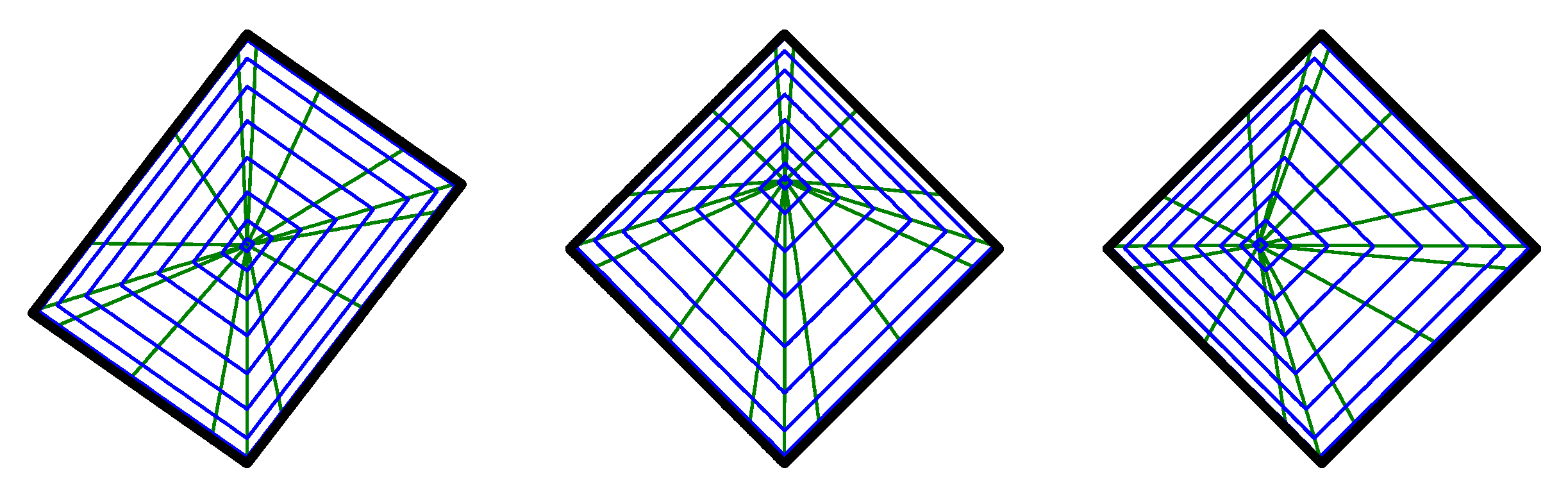
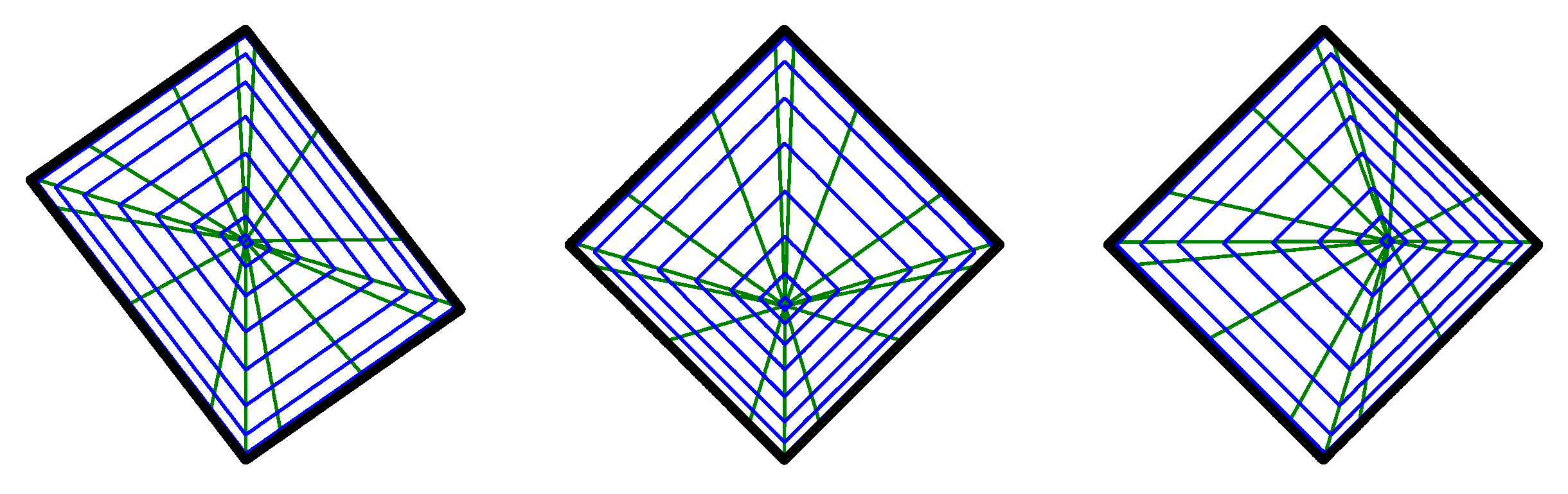
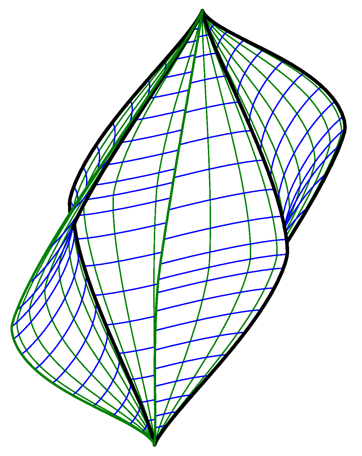
In Figure 5, we show special cases. On the left, we show a sphere in the norm of $b{v}_0$, for the parameters $d_1=d_2=d_3=1$, in the middle in the norm of the original Hahn space h, for the parameters $d_1=1$, $d_2=2$, $d_3=3$, and on the right in the norm of the generalized Hahn space $h_d$ with the parameters $d_1=1.2$, $d_2=1.5$, $d_3=4$. All the exponents are equal to one, and the matrix A is:

$$A=\left(\begin{array}{ccc}{d}_1& -d_1& 0\\ & d_2& -d_2\\ & & d_3\end{array}\right).$$

Figure 5. Special cases. (left): $b{v}_0$ space. (middle): original Hahn space h. (right): generalized Hahn space $h_d$.

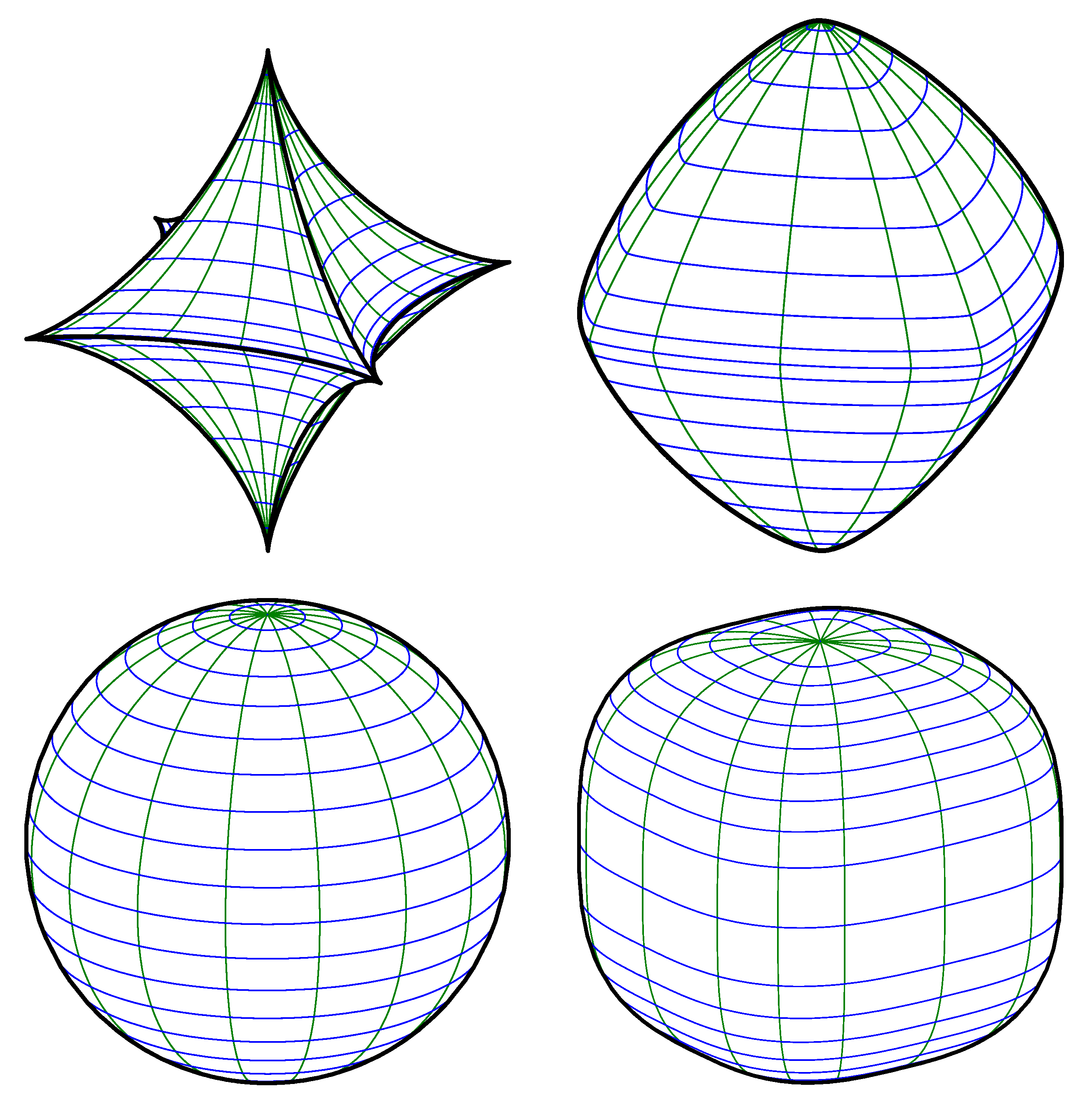
Varying the exponents $p_k$ results in a change of the shape of the spheres. We show the unit sphere with identity matrix A.

First, we considered spheres with equal exponents in each sphere. Figure 6 shows the unit spheres with the exponents $p=p_k$ for $k=1,2,3$, where $p=0.7$, $1.3$, 2, and 3, that is with respect to the metric of ${\ell }_{0.7}$, and the norms of ${\ell }_{1.3}$, ${\ell }_2$, and ${\ell }_3$. Left on the bottom is the ordinary Euclidean sphere.

Figure 6. Spheres with respect to the metric of ${\ell }_{0.7}$ and the norms of ${\ell }_{1.3}$, ${\ell }_2$, and ${\ell }_3$.

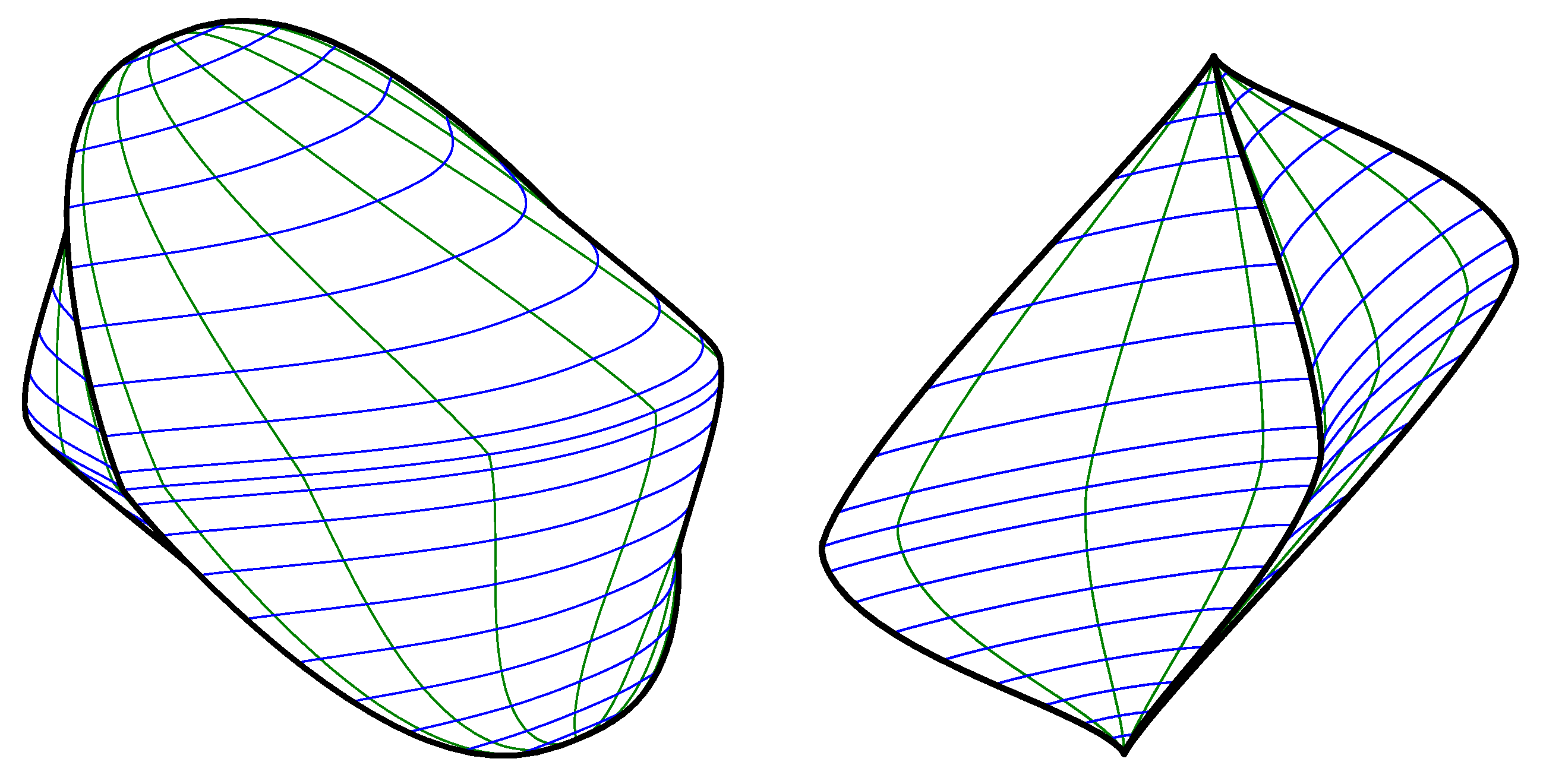
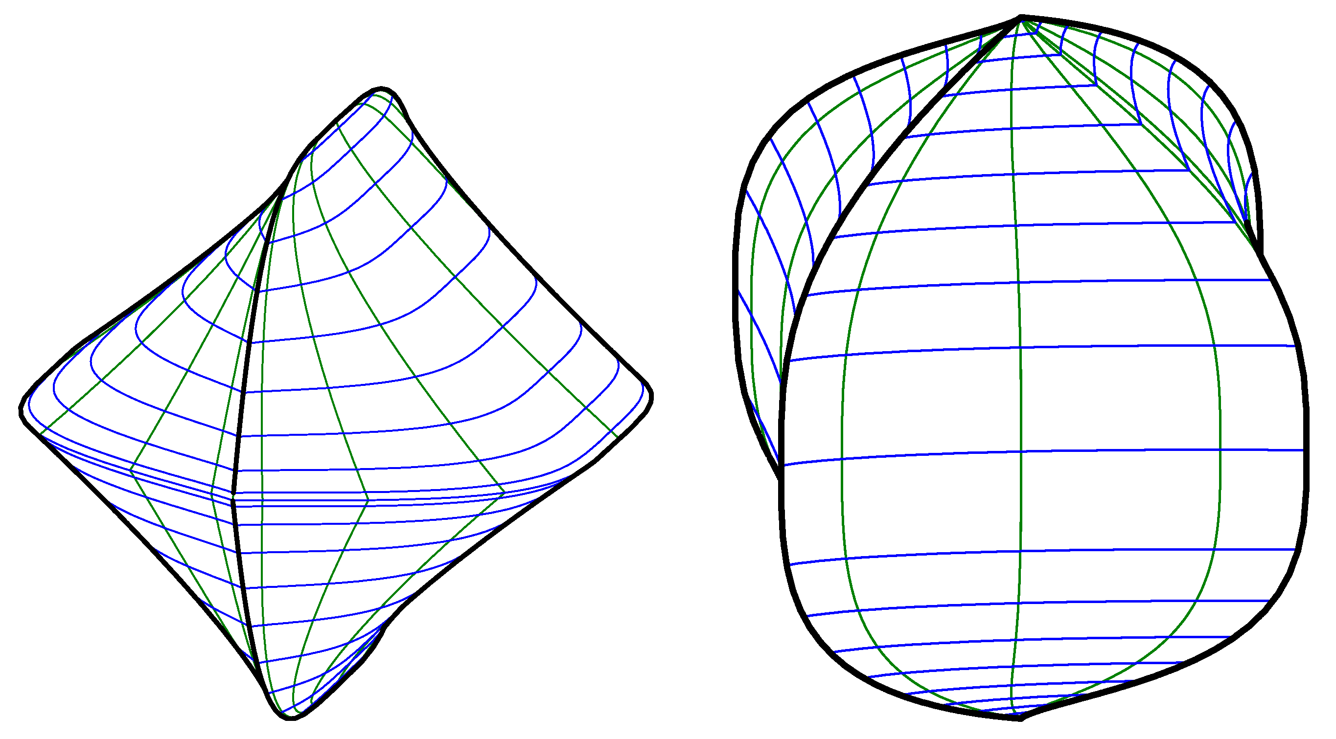
If the exponents are different, the shape of the sphere is more interesting. We considered the unit sphere with the identity matrix A. On the left in Figure 7, the exponents are $p_1=4$, $p_2=0.8$, $p_3=1$, and on the right, they are $p_1=1$, $p_2=0.8$, $p_3=3$.

Figure 7. Different exponents: (left) $p_1=4$, $p_2=0.8$, $p_3=1$; (right) $p_1=1$, $p_2=0.8$, $p_3=3$.

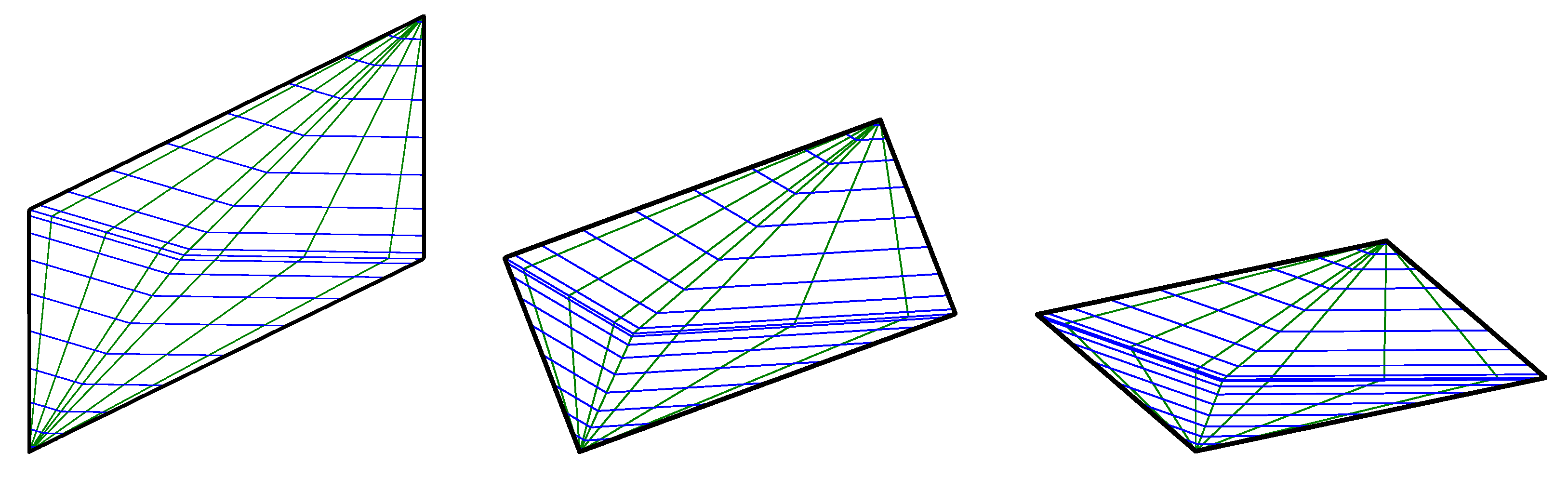
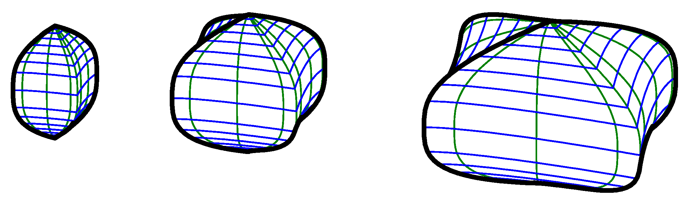
Now, we demonstrate the influence of the radius. In Figure 8, we chose the spheres with identity matrix A and the exponents $p_1=1$, $p_2=0.8$, $p_3=3$. The radii vary from left to right with the values $0.9$, $1.1$, and $1.3$. We observed that not only the size increased, but the spheres also stretched out differently in different dimensions due to the exponents. Note that the same sphere of radius one is shown on the right side of Figure 7.

Figure 8. Spheres of radii $0.9$, $1.1$, and $1.3$ and exponents $p_1=1$, $p_2=0.8$, $p_3=3$.

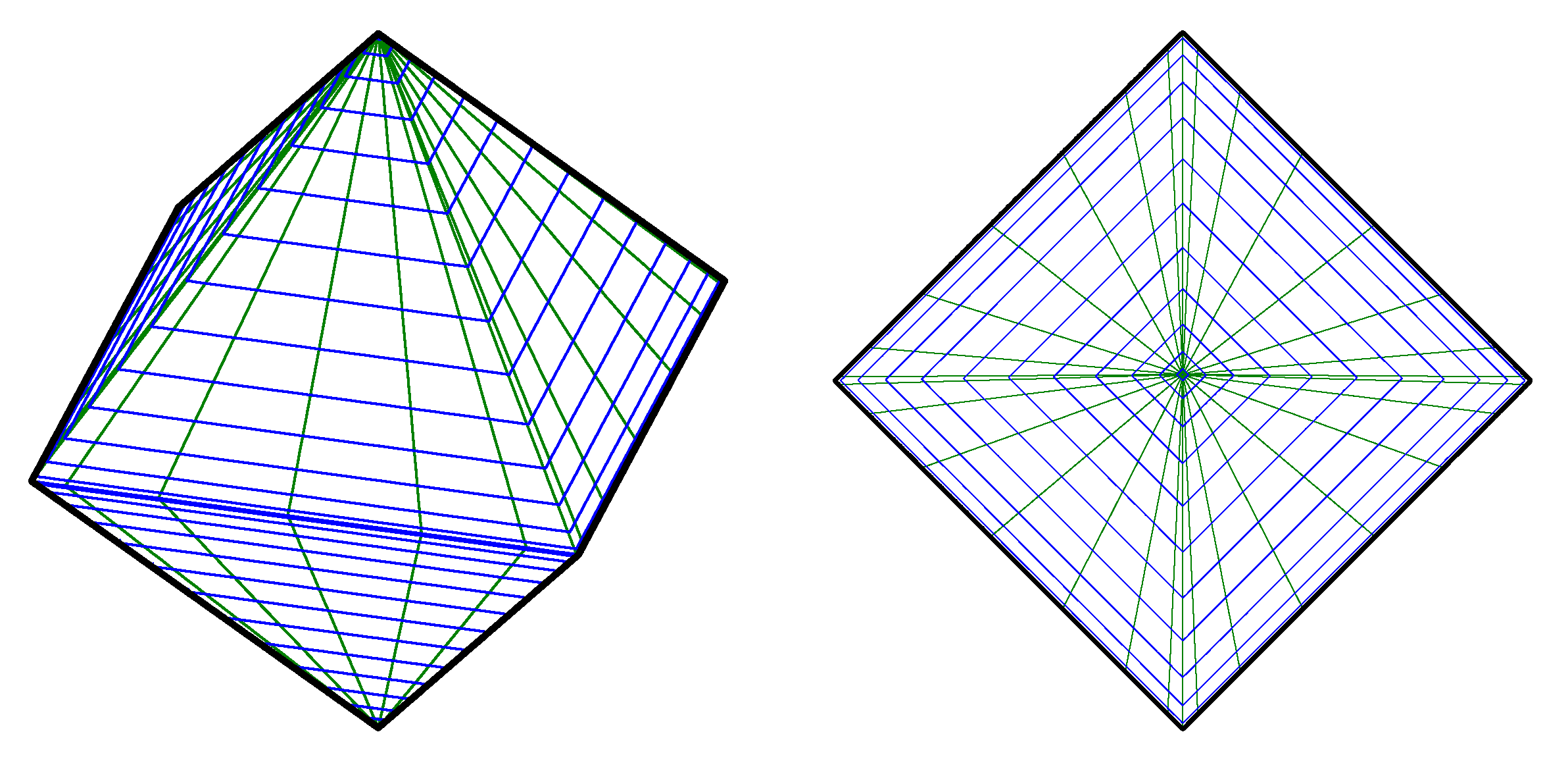
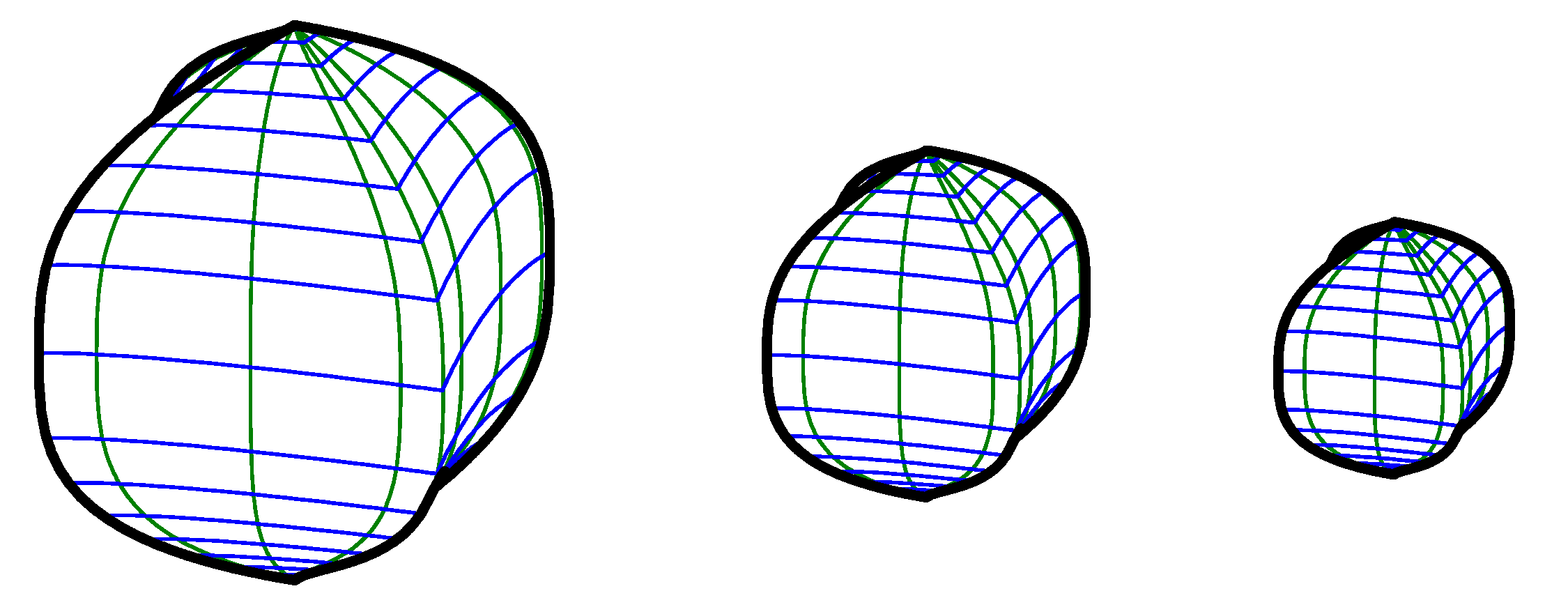
Now, we consider the case when A is a diagonal matrix, but not the identity.

In Figure 9, the exponents are $p_1=1$, $p_2=0.8$, $p_3=3$, as on the right in Figure 7 and Figure 8. However, now, the values on the diagonal are equal to $0.5$ in the diagonal matrix A on the left, $0.8$ in the middle, and $1.1$ on the right. Note that as the entries increase, the sizes of the spheres decrease, but their shapes do not change.

Figure 9. Entries of the diagonal matrix A equal to $0.5$ (left), $0.8$ (middle), and $1.1$ (right).

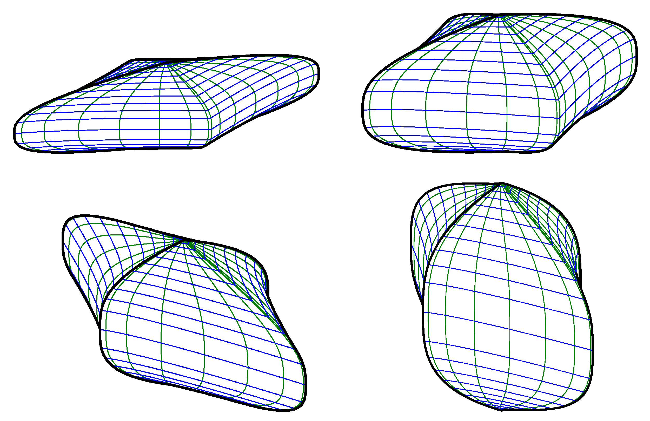
In Figure 10, the exponents are the same as in the previous figure, $p_1=1$, $p_2=0.8$, $p_3=3$, but the values on the diagonal of the matrix A are different:

$$\mathrm{Top} \mathrm{left}:A=\left(\begin{array}{ccc}0.5& 0& 0\\ & 1& 0\\ & & 2\end{array}\right).\mathrm{Top} \mathrm{right}:A=\left(\begin{array}{ccc}0.6& 0& 0\\ & 0.8& 0\\ & & 1.3\end{array}\right).$$

$$\mathrm{Bottom} \mathrm{left}:A=\left(\begin{array}{ccc}2& 0& 0\\ & 0.8& 0\\ & & 2.5\end{array}\right).\mathrm{Bottom} \mathrm{right}:A=\left(\begin{array}{ccc}4& 0& 0\\ & 2& 0\\ & & 3\end{array}\right).$$

Figure 10. Entries on the diagonal of each diagonal matrix A are different.

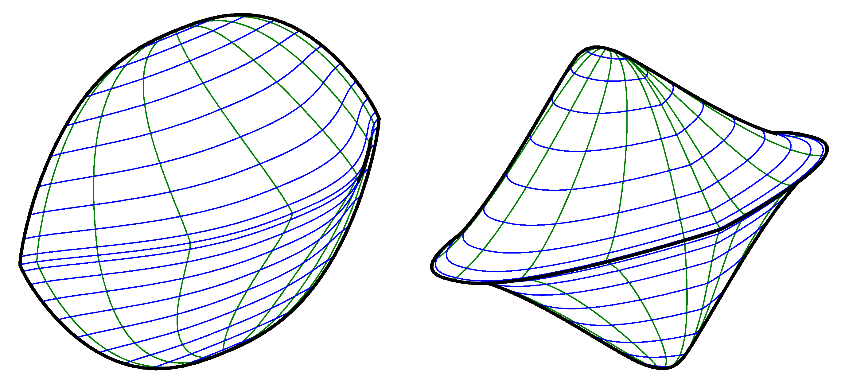
We can also change the entries of the matrix A and the exponents $p_k$ at the same time. On the left in Figure 11, the exponents are $p_1=2.5$, $p_2=0.8$, $p_3=1.2$, and on the right, they are $p_1=0.8$, $p_2=0.8$, $p_3=1.5$. The matrices are:

$$\mathrm{Left}:A=\left(\begin{array}{ccc}2& 1& -0.5\\ & 3& 1\\ & & 2\end{array}\right).\mathrm{Right}:A=\left(\begin{array}{ccc}2& -0.2& 0.3\\ & 5& -0.2\\ & & 3\end{array}\right).$$

Figure 11. Different entries of matrix A and different exponents $p_k$.

Figure 1 is part of the sphere on the right in Figure 11.

Finally, on the left in Figure 12, the exponents are $p_1=2.5$, $p_2=0.7$, $p_3=1.2$, and on the right, they are $p_1=1.1$, $p_2=2.5$, $p_3=0.7$; the matrices are the same:

$$A=\left(\begin{array}{ccc}2& 0.2& -0.5\\ & 5& -0.2\\ & & 3\end{array}\right).$$

Figure 12. The same matrix A, but the exponents are different.

6. Conclusions

We introduced the generalized Hahn space $h_A\left(p\right)$ for upper triangle matrices A and sequences $p={\left(p_k\right)}_{k=1}^{\infty }$ of positive real numbers and showed that $h_A\left(p\right)$ is a linear metric space with its natural paranorm, if the sequence p is bounded. We also noted that $h_A\left(p\right)$ need not be a linear space, if the sequence p is unbounded.

We applied our own software to visualize the shapes of parts of spheres in three-dimensional space endowed with the relative paranorm $h_A\left(p\right)$. Furthermore, we developed the parametric representation of these spheres and solved their visibility and contour (silhouette) problems. Finally, we demonstrated the effects of the change of the matrices A and the sequences p on the shape of the spheres.