Super Resolution for Noisy Images Using Convolutional Neural Networks

Abstract

The images in high resolution contain more useful information than the images in low resolution. Thus, high-resolution digital images are preferred over low-resolution images. Image super-resolution is one of the principal techniques for generating high-resolution images. The major advantages of super-resolution methods are that they are economical, independent of the image capture devices, and can be statically used. In this paper, a single-image super-resolution network model based on convolutional neural networks is proposed by combining conventional autoencoder and residual neural network approaches. A convolutional neural network-based dictionary method is used to train low-resolution input images for high-resolution images. In addition, a linear refined unit thresholds the convolutional neural network output to provide a better low-resolution image dictionary. Autoencoders aid in the removal of noise from images and the enhancement of their quality. Secondly, the residual neural network model processes it further to create a high-resolution image. The experimental results demonstrate the outstanding performance of our proposed method compared to other traditional methods. The proposed method produces clearer and more detailed high-resolution images, as they are important in real-life applications. Moreover, it has the advantage of combining convolutional neural network-based dictionary learning, autoencoder image enhancement, and noise removal. Furthermore, residual neural network training with improved preprocessing creates an efficient and versatile single-image super-resolution network.

1. Introduction

Digital images captured by poor resolution cameras have three primary limitations, namely aliasing, blurring, and noise. Aliasing can occur due to inadequate image sensor elements that lead to an under-sampled spatial resolution, which results in a significant loss of high-frequency (HF) information, such as edges and textures. Image blur occurs due to camera motion, jitter, out-of-focus, etc. In addition to blur, various noises can also be added to the image during the imaging process and can degrade the image quality. Degradation may also occur because of the sensor element’s point spread function (PSF). Super-resolution (SR) refers to those techniques designed to build high-resolution (HR) images from single or more observed low-resolution (LR) images by increasing the HF components, replicating larger dimensional multipliers, and removing the degradation caused by the low-resolution camera imaging process. In essence, the super-resolution process should reconstruct lost HF details while minimizing aliasing and blurring. As stated before, HR images are obtained by increasing the number of image sensor elements and reducing the pixel size. This increases the pixel density. However, a reduction in pixel size causes shot noise and degrades the quality of the image captured. In addition, it may result in additional costs due to an increase in the number of sensor elements. Therefore, the employment of novel signal processing approaches is required to post-process the captured LR images. A simple approach is by interpolating the LR image to the size of the desired HR image. However, traditional interpolation approaches, such as bilinear, bi-cubic, and nearest neighbor algorithms, result in blurry images, as the missing pixel is found by averaging it from a neighboring pixel. The blurry effect introduced by interpolation techniques contributes to the loss of HF details, and hence, the fundamental problem in SR reconstruction, i.e., aliasing effect (loss of HF details), remains unsolved. Typically, an image that holds fine details is said to be an HR image and that with fewer details is referred to as an LR image. Image resolution provides the least measure of detail with which an image can be resolved into a more intricate and clearly defined pixel. As the resolution of an image is increased, it conveys a more complex structure. Therefore, image resolution is vital in all wings of digital image processing, and the performance of an image-processing algorithm depends on image resolution. It is therefore one of the key aspects of digital image processing. The resolution of an image depends primarily on the sensor elements used in the imaging device. For obtaining an HR image, a sophisticated, complex sensor is therefore needed. This can be very expensive and, in many cases, not affordable. Resolution is an important term for the quality assessment of image acquisition and processing devices in digital image processing. Image resolution is defined as the smallest measurable visual data in an image. The resolution of an optical device can be quantified by measuring its OTF, which is a measure of the system response to different spatial frequencies. Digital image processing can generally classify the image resolution into the following four types:

(1)

Pixel or Spatial Resolution: An image consists of several distinguishable pixel image elements. The spatial distance between pixels in an image is called pixel or spatial resolution. The first number is the number of pixel columns (width), while the second is the number of pixel lines (high), named m by n. It is represented by a set of two positive integers. High spatial resolution improves the image quality by allowing a clear insight into fine details and vivid color transitions. Instead, an image with fine details not shown with enough pixels suffers from aliasing and introduces undesired artifacts, such as the blocking effect.

(2)

Intensity Resolution: The number of grey levels used to represent an individual pixel is referred to as intensity resolution. It is represented by the number of bits used to represent each intensity level. A small, discernible change in grey level can be perceived with a large number of bits used to represent a pixel. However, increasing the number of bits increases the image size. A monochromatic image’s typical intensity resolution is 256 grey levels, implying 8 bits are required to represent a pixel.

(3)

Temporal Resolution: Temporal resolution refers to the frame rate captured by a camera in a motion picture. It carries the motion information between two subsequent frames. Movements in a scene can be viewed without smearing using a higher frame rate. A typical frame rate to view motion pictures is above 25 frames per second.

(4)

Spectral Resolution: The ability to resolve an image into its respective frequency or spectral components is known as a spectral resolution. However, spectral resolution is not discernible to human eyes as much as spatial resolution. Hence, the spectral analysis generally allows a higher tolerance range since small changes in the spectral resolution often go undetected.

The modern image sensor element is typically an active pixel sensor or a Complementary Metal-Oxide-Semiconductor. Typically, the sensor elements are arranged in a two-dimensional array for images. The sensor element size or the number of sensor elements present in the unit area determines the spatial resolution of an image. An imaging device with poor sensors produces LR images with visual artifacts that are blocky and displeasing as a result of the aliasing effect. However, the use of a large number of hardware components to increase spatial resolution also increases costs, which is a major concern for many commercial imaging applications. Furthermore, there are two limitations to deploying high-precision optics in imaging devices. In addition to unwanted increases in costs, customers’ continuous demand for increased resolution cannot be met by the technology due to their technical restrictions on sensor size, shooting noise, etc. Alternative methods to improve the current resolution level are therefore essential. The reduction of pixel size by sensor manufacture technologies is a direct solution for improving spatial resolution. However, the volume of incoming light-per-pixel unit decreases as the pixel size decreases. This creates a shot noise that decreases the quality of the image. This becomes a major concern when the pixel size is reduced [1]. Another way to improve spatial resolution is to increase the size of the chip. However, as the chip size grows, so does the capacitance [2]. This method is ineffective because increasing the charge transfer rate is difficult due to increased capacitance. However, the sensor element limits the spatial image resolution its optics, i.e., lens blur, aberration effects, aperture diffraction, and optical blurring due to motion, etc. It also limits the fine details in the image. Building imaging chips and optical components to capture HR images is prohibitively expensive and impractical in the majority of real-world applications. A new, cost-effective approach is therefore preferred for increasing the spatial resolution of an image to resolve the limitation due to the production of lenses and sensors. A promising approach is to use resolution enhancement techniques to post-process the acquired LR image. Because these techniques are applied to previously acquired images, they are flexible and cost-effective because no additional hardware components are required.

2. Preliminaries and Related Works

Super-resolution (SR) is a classical image-processing problem that has been explored since the original work that Tsai and Huang reported in 1984 [3] for over two decades. The term super-resolution was reported in the literature by Irani and Peleg in 1991 [4]. The field of image SR garnered special interest by researchers in the late eighties and early nineties and has witnessed numerous SR algorithms under various categories. Comprehensive reviews and surveys on the SR problem are reported in the literature [5,6,7,8]. Early studies employ interpolation methods, such as bicubic interpolation and discrete cosine transform (DCT) interpolation. To upsample low-resolution images, the most advanced method is to use a deep-learning-based convolution neural network (CNN). Dong et al. [9] created a 3-layer CNN model called Super-Resolution Convolution Neural Network (SRCNN) to achieve end-to-end mapping between low- and full-resolution images. They also demonstrated the connection between SRCNN and sparse-coding-based methods [10]. SRCNN model shows great improvement in accuracy compared with interpolation methods or sparse-coding-based methods. Kim et al. [11] went one step further by designing a very deep CNN model named VDSR. Different from [9], in [11], the authors dropped the structural mapping to sparse-coding-based methods. Instead, they increased the number of CNN layers to 20 and proved that deeper networks could dig out more useful information and further increase the accuracy. Besides, they used the concept of residual learning by adding a shortcut from input to output into the CNN model. Current research on image super-resolution can be classified into two classes: One class is to further improve the accuracy by making modifications to the deep neural network structure. Kim et al. [12] proposed a deeply-recursive convolution network (DRCN) based on the VDSR model. It also uses a 20-layer convolution network, but the difference from VDSR is that in DRCN, there are several recursive layers, and these recursive layers share the same filter kernel. Testing results show that DRCN can further improve the performance over VDSR by a small degree. Another class is to explore shallow convolution networks with equally good performance and less computation cost. Li et al. [13] designed a 5-layer residual neural network for upsampling and coding artifacts removal. This network is much shallower than VDSR. It adopts multi-scale feature extraction by using multi-scale filter sizes in the second and fourth layers. Classical multi-image SR uses LR pixels from multiple LR images to create an HR image, while single-image SR extracts LR patches from a single LR image and uses them to reconstruct an HR image of the same scene with LR image [14]. The framework of sparse representation for single-image SR [15] focuses on these two constraints and finds their sparse representation to reconstruct the final HR image. Reconstruction constraints [15] is shown in Equation (1) as follows:

$$Y=D_S B_{f }X$$

(1)

where $D_S$ represents down-sampling operator, $B_{f }$ blurring filter, and $X$ is upsampled and deblurred version of $Y$.

The foundation for the convolutional neural network for single-image super-resolution is a paper titled “Learning a Deep Convolutional Network for Image Super-Resolution” (SRCNN) [16], by C. Dong et al. Convolutional neural networks (CNN) are used to map the low-resolution image LR to the high-resolution image HR end-to-end. Instead of taking each feature component one by one in the dictionaries like traditional sparse coding methods [15], SRCNN optimizes all layers at one time. SRCNN optimizes all layers at one time. As a result of this process, fast and better image quality is obtained with the SRCNN method. The SRCNN consists of the following three main steps:

• Patch extraction: The first layer is defined as a function set, F1, as shown in Equation (2) [16]. These functions are used to extract image patches by convolving the image.

$$F_1\left(Y_{lr}\right)=MAX\left(0,W_1 Y_{lr}+B_1\right)$$

(2)

where $Y_{lr}$ represents the input LR image, $W_1$ is filters, and $B_1$ is biases. The size of $W_1$ is c × f1 × f1 × n1, where c represents the number of image channels, f1 is the size of filter, and n1 is the number of convolution filters.

Additionally, the Rectified Linear Unit (ReLu) is applied to the filter output.

2.

End-to-end non-linear mapping: In this process, one high-dimensional image is mapped onto another vector. Each non-linearly mapped vector represents a HR image patch. Equation (3) [16] defines the second layer as:

$$F_2\left(Y_{lr}\right)=MAX\left(0,W_2 F_1{Y}_{lr}+B_2\right)$$

(3)

where $B_2$ represents n2-dimensional vector, and $W_2$ is filters with n1 × 1 × 1 × n2 size.

Each n2-sized vector represents a HR image patch. Then, these vectors are used to reconstruct the final HR image.

3.

Reconstruction: In this layer, the generated overlapping HR patches are averaged to create the final HR image. The construction step is defined with a convolution layer, which is presented in Equation (4) [16]:

$$F\left(Y_{lr}\right)=W_3\times F_{2 }{Y}_{lr}+B_3$$

(4)

where $B_3$ is a vector with c-dimensional, and the size of $W_3$ is n2 × f3 × f3 × c.

Although the popularity of sparse-coding-based algorithms has declined following the dominance of deep learning and CNN in the single-image super-resolution (SISR) area, sparse-coding-based network (SCN) [17] and its advanced work, “Learning a Mixture of Deep Network for Single Image Super-Resolution” (MSCN) [18], demonstrate that sparse coding can be much more efficient when combined with appropriate deep learning methods. SCN and MSCN not only improve efficiency and training, but they also reduce the model size, resulting in better performance with fewer parameters when compared to other sparse coding methods [19]. Hyperparameter tuning is a well-known method for improving the accuracy or performance of any machine learning model [20,21]. The MSCN network consists of SR in reference modules and one adaptive weight module, which are applied to LR images to obtain one HR image. Then, all predicted HR images are combined in the aggregation layer by using an adaptive weight module [18]. He et al. proposed a ResNet [22] for image classification. Its key idea is to learn residuals through global or local skip connections. It notes that ResNet can provide a high-speed training process and prevent the gradient vanishing effects. L.Dong et al. [23] proposed a simple yet effective self-encoder denoising network based on CNNs that can be taught end-to-end unattended. The network was designed using a fully convolutional auto-encoder with symmetrical encoder-decoder links. Not only can the proposed approach reconstruct clean images from corrupted photographs, but it can also be trained to display abstract image representation through reconstruction training. The works, such as “Super-resolution and noise filtering with moving least squares” [24], make use of the Discrete Fourier Transform (DFT), the Discrete Cosine Transform (DCT), or the Discrete Wavelet Transform (DWT) of LR images to recover missing high-frequency components in HR images. Regularization methods for image SR employ either standard stochastic or deterministic regularization techniques when there is a limited number of input LR images. This strategy incorporates prior limited information about unknown HR images [25]. Feature selection helps to reduce the dimensionality of a feature vector by removing redundant and irrelevant features [26]. Theoretical and practical global optimization problems have prompted the development of swarm intelligence approaches [27].

The study of the above literature shows the variety of approaches used to perform SR. When there is one single LR image, example-based SISR techniques that learn the connection between LR and HR images from exemplary pairs automatically show good results. In particular, recent progress in neural networks makes these approaches appropriate for this purpose. They can be trained on enormous amounts of data and analyze images in a single forward pass, eliminating the need to search online (for example, for the nearest neighbor) or optimization methods.

A model for the single-image super-resolution problem is presented in this paper. In addition, an attempt is made to solve the problem by training the model on the low- and high-resolution image(s) using Convolutional Autoencoder and Residual Neural Network models based on Convolutional Neural Network to generate a higher-resolution image when a lower-resolution image is given to the model after training it. Details of the proposed method are explained in Section 2. Section 3 explains the methodology of our proposed method. Section 4 presents various experiments to test the proposed method and describes implementing details with the result of the simulations Then Section 5 concludes the proposed method along with the future enhancements.

3. The Proposed Work

There are various SR algorithms, and they have advantages over one another. Although more complicated deep neural network models have demonstrated better SR performance than conventional methods, it is difficult to implement them on low-complexity, low-power, and low-memory devices due to the massive network parameters and convolution operations of deeper and denser networks. In the case of SR-DenseNet, it is difficult to implement this model to the applications for real-time processing even though its SR performance is superior to that of other neural network models. Further, due to GPU limitations, we cannot implement a denser and deeper Convolutional Neural Network. To address this issue and perform the task of single-mage super-resolution while keeping the resources and aim of this project in consideration, a hybrid model was created by concatenating two separate models. A CNN learning-based deep network method is proposed for a single-image super-resolution framework. In addition, it was ben observed that convolutional autoencoders and deep residual neural networks show better performance for high-resolution image reconstruction.

The proposed method is a combination of two existing state-of-the-art models. It has been noticed that the convolutional autoencoders perform well when it comes to removing noise from an image or enhancing it. Furthermore, it has been observed that abstract image representation through the reconstruction training and residual neural networks provide a high-speed training process. However, when the model is about to converge, it prevents the gradient vanishing effects and tackles the problem where the accuracy of networks with many numbers layers rapidly decreases. Hence, a method is proposed that concatenates the above methods with improved preprocessing steps to create a higher-resolution image from a lower-resolution image.

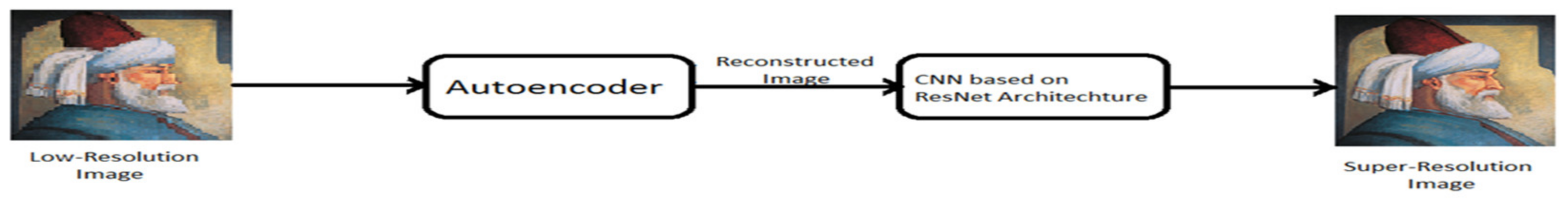
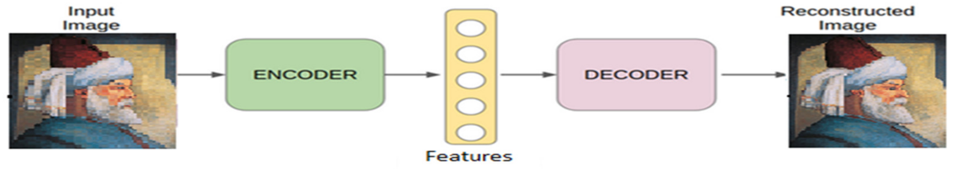
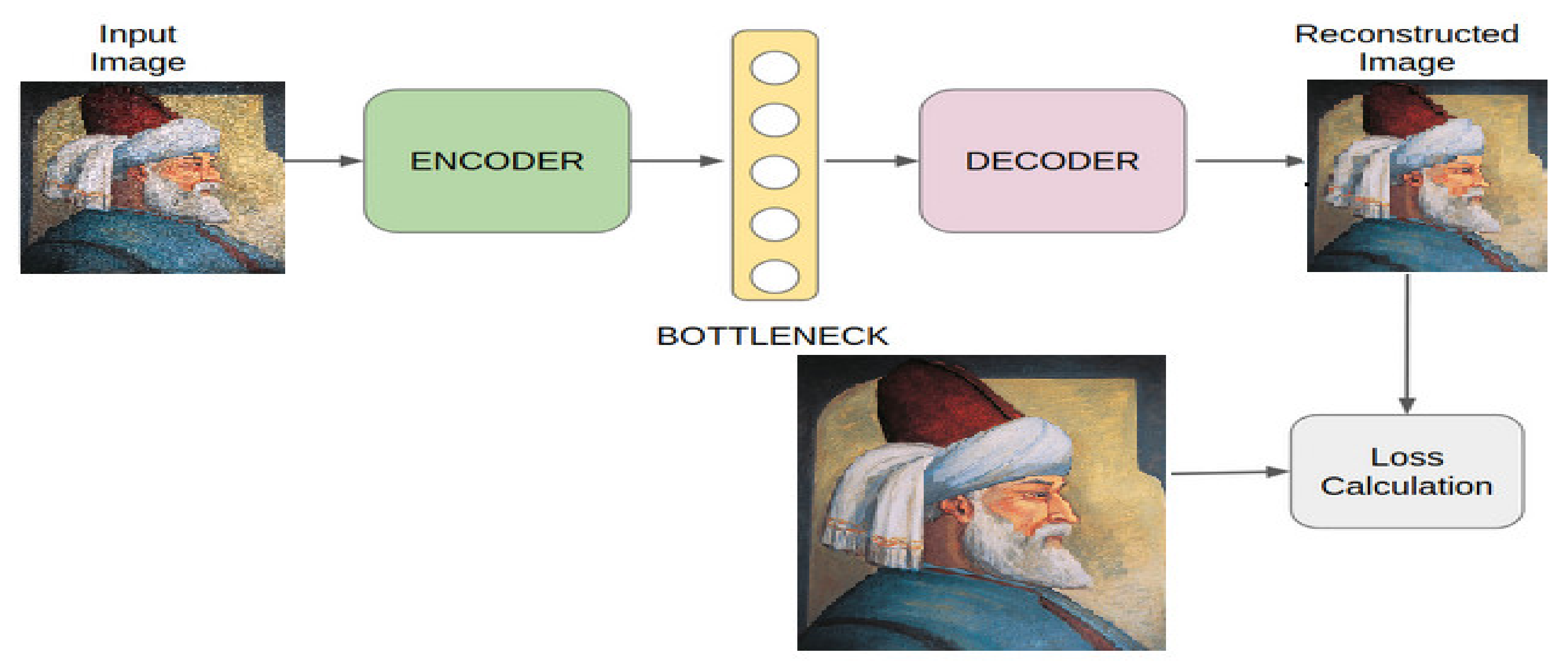
The framework of the proposed model is shown in Figure 1. The aim of this model is to create a higher-resolution from a lower-resolution input image. Firstly, the lower-resolution image is given to the convolutional autoencoder, which is comprised of two connected networks—encoder and decoder. A simplified autoencoder model is given in Figure 2.

Figure 1. Framework of proposed model.

Figure 2. Autoencoder model.

The encoder takes the input low-resolution image and exacts features from it. This network is trained in such a way that the features extracted by the encoder can be used by the decoder to reconstruct an image that has lesser noise in it. Furthermore, it is also more enhanced than the lower-resolution input image, giving us the super-resolution type of the original image.

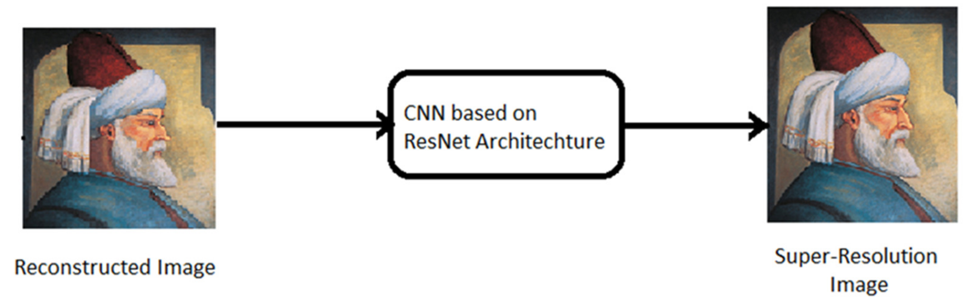
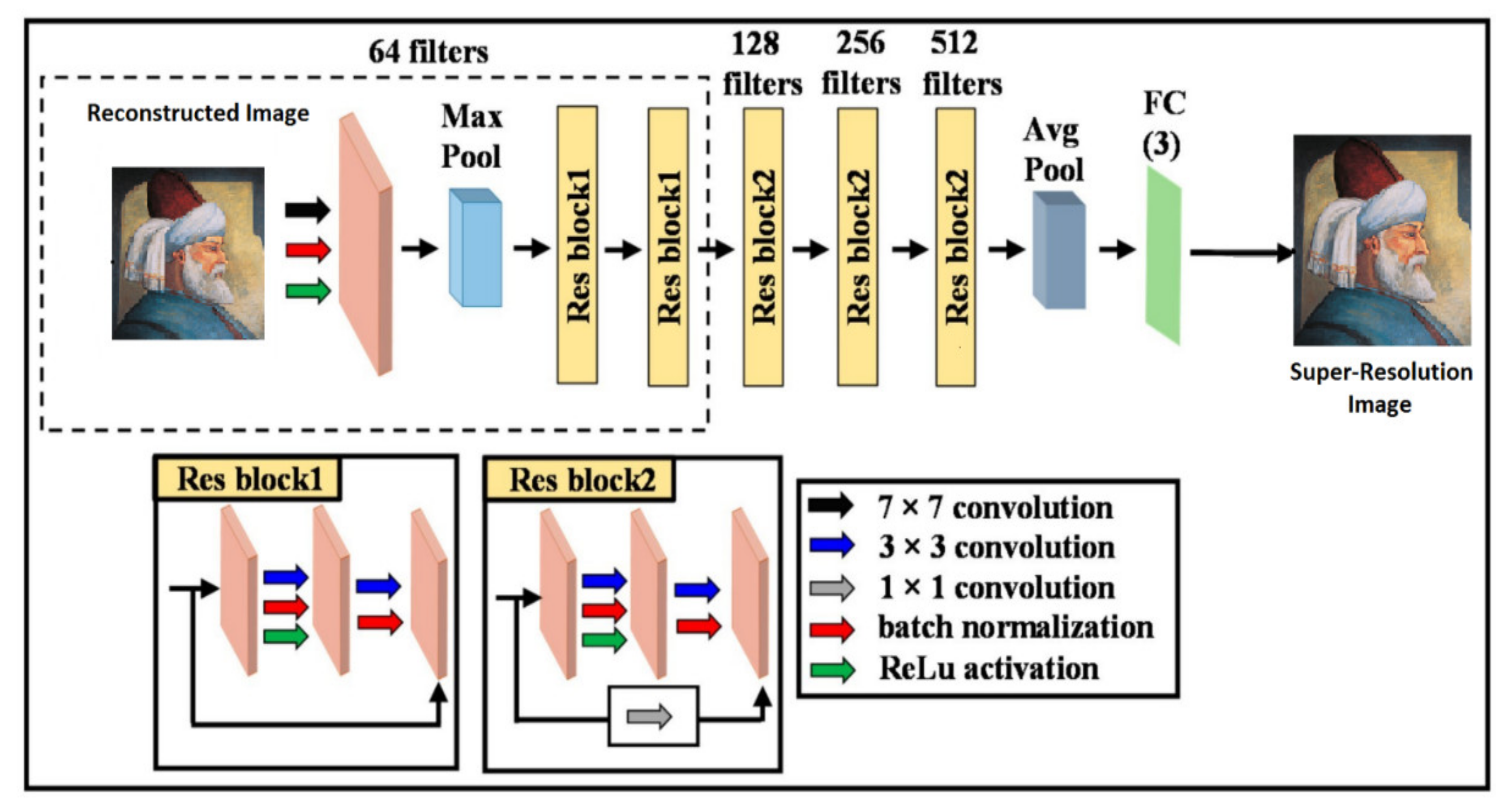
As shown in Figure 3, the reconstructed image is then passed to the CNN based on ResNet architecture, which further processes the reconstructed images obtained from the convolutional autoencoder, using various residual learning blocks, and creates a higher-resolution image, which provides more detail and information about the image. The next section explains the proposed method step by step and the methodology involved in it.

Figure 3. Input and Output of ResNet based CNN.

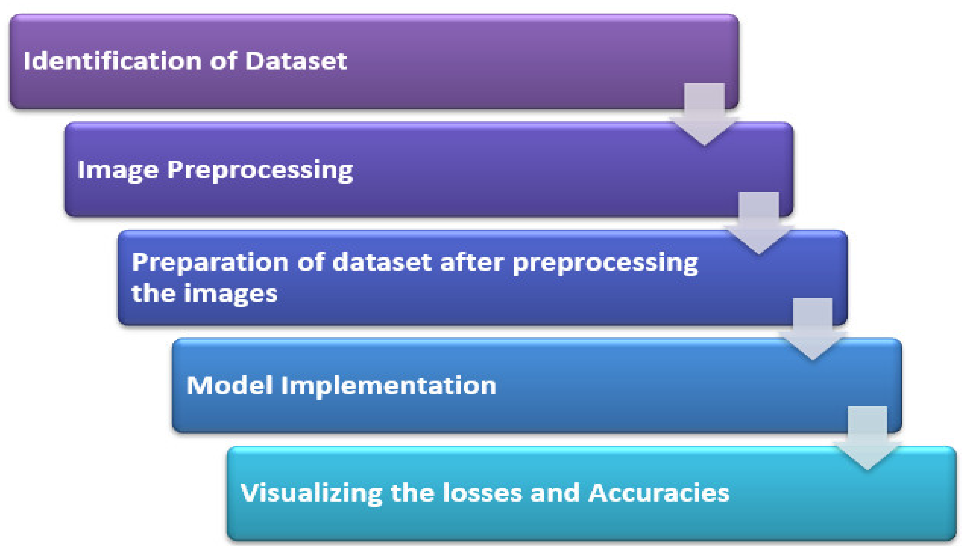
4. Methodology

After providing a detailed motivation for designing the proposed model for SISR, this section describes the structure and the implementation of the proposed model in a stepwise manner as shown in Figure 4.

Figure 4. Methodology.

4.1. Identification of Dataset

For the good performance of the model, the dataset should be large enough for the model to be trained on it for learning purposes. There are many datasets available on the Internet that contains hundreds and thousands of images, e.g., The General-100, BSD-300, BSD-500, DIV2K, ImageNet dataset, etc., and these can be used for the task of SISR.

Various datasets were selected for training our model, such as the LFW (Labelled Faces in the Wild) dataset, which is commonly used for studying the problem of unconstrained face recognition. It has been used to test how well our model will perform on facial images of people, especially the encoder part of our model, BSD-300 (Berkeley Segmentation Dataset), which is used by our model for training on image denoising and performing super-resolution. A dataset of our own was created, which included images from these datasets and other images from the Internet for diversification of our dataset. Our dataset contains around 1000 HR images that can be used for obtaining low-resolution images after performing various image preprocessing operations on them. These high- and low-resolution images can then be used for training and validation of our models only after applying a pre-processing step on a given set of images.

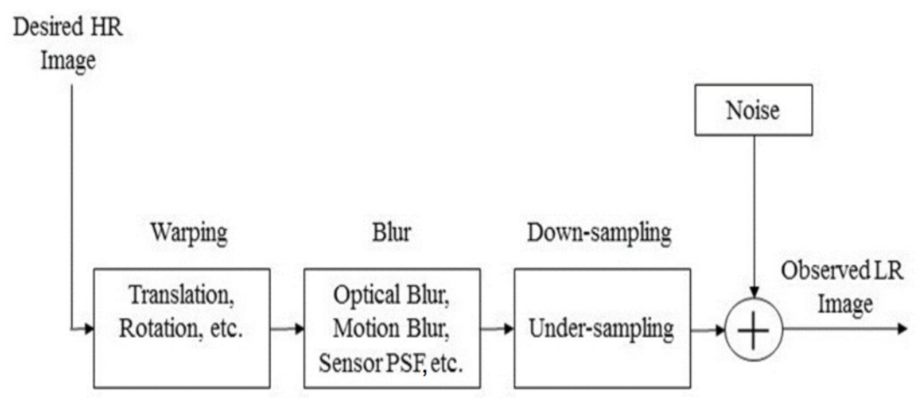
4.2. Image Preprocessing

This step involves the degradation of an unknown HR image for obtaining the observed LR image. The success of SR algorithm essentially depends on the LR image formation model since it relates the observed LR image with its unknown HR image. The most common model is based on aliasing, blurring, warping, down-sampling (under-sampling), adding noise, and shifting of the original HR image. A simplified LR image formation model is shown in Figure 5.

Figure 5. Image degradation step.

From this step, it was demonstrated that low-resolution images from high-resolution images can then be used for training and validating our models with high-resolution images. Thus, in this way, the model is trained on the input images and output images in a supervised fashion as shown in Figure 6.

Figure 6. Images after image-degradation step.

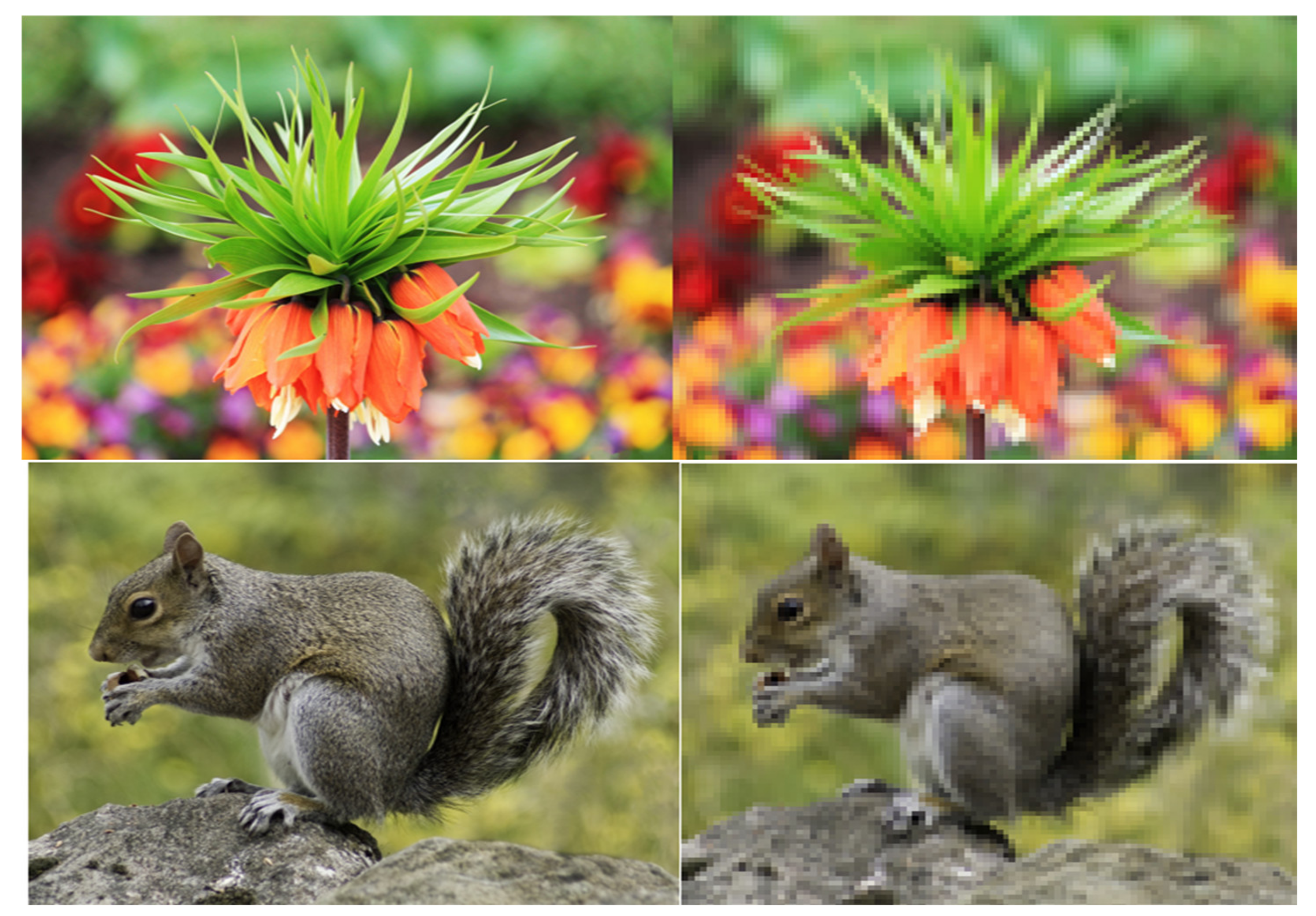
4.3. Preparation of Dataset after Preprocessing the Images

After obtaining data from various sources and performing some image modifications, i.e., adding noise elements and other distortion to the input images, our dataset was divided into two categories, namely high-resolution and low-resolution images. The way these images are loaded into the model is as low-resolution images, which act as the input feature, and with their counterpart high-resolution images as the desired output images for training and validation. The model learns to map the low-resolution image to its high-resolution counterpart. Each high-resolution image contains its low-resolution counterpart, which can be used by our model for learning and training. Some images from the dataset are given in Figure 7.

Figure 7. High-resolution and their lower-resolution images.

4.4. Model Implementation

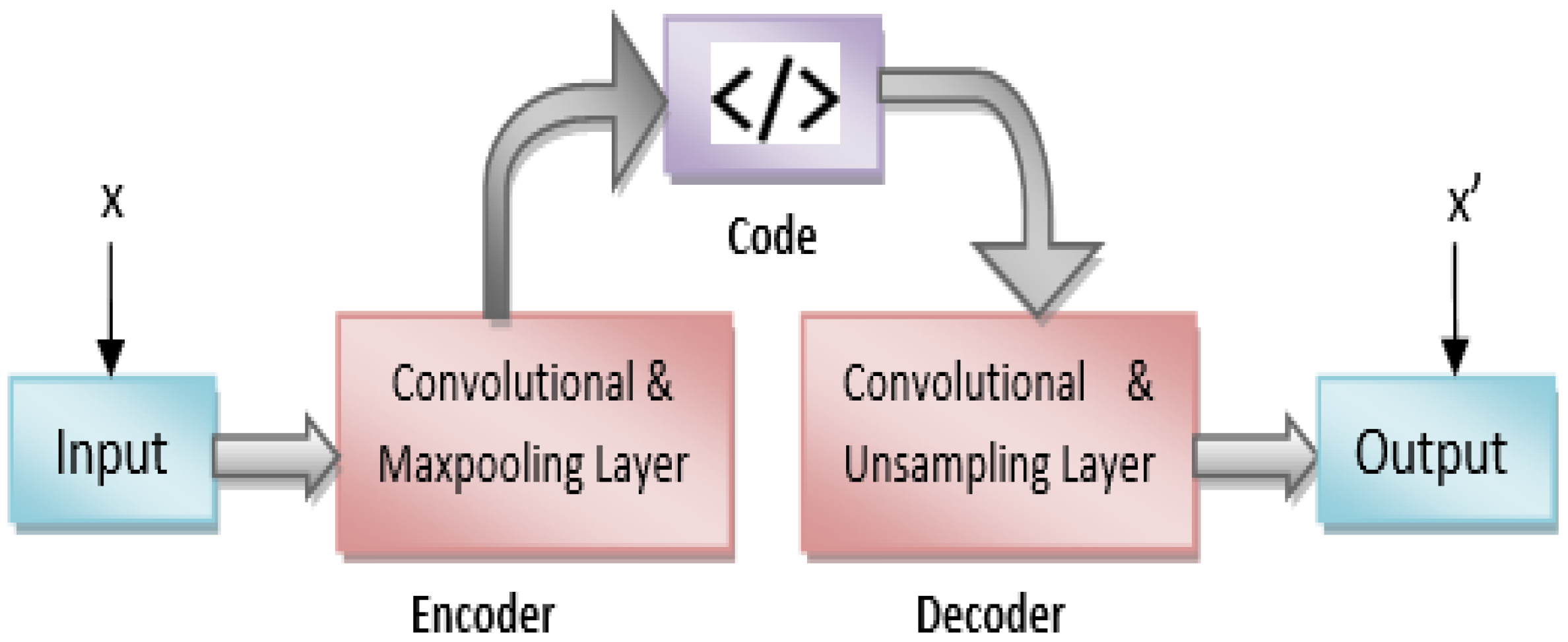
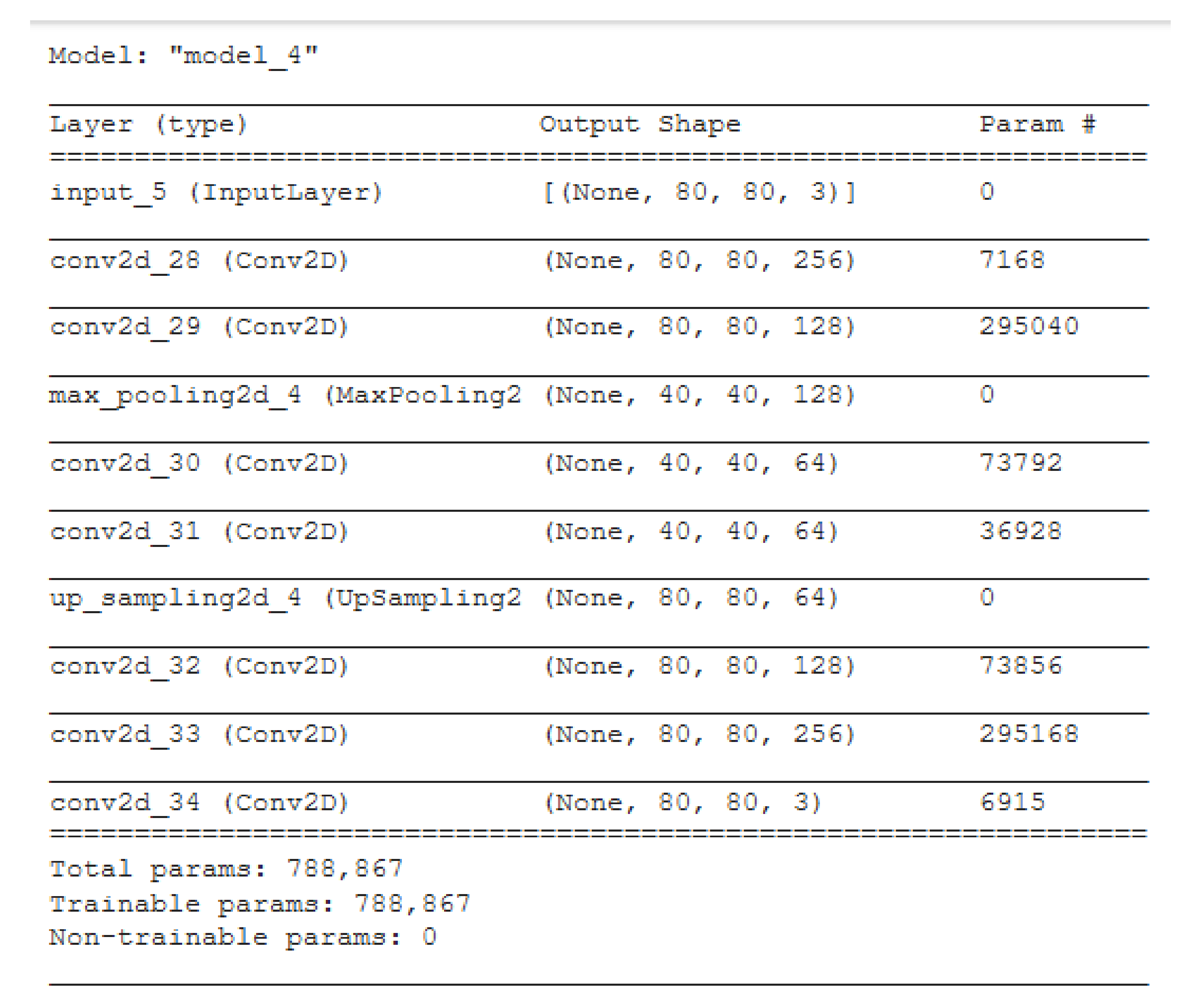
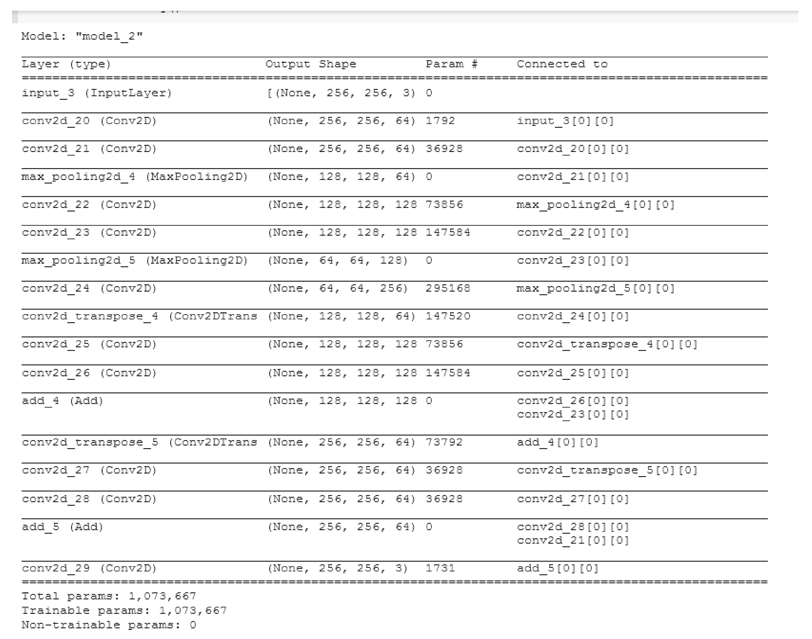
After preparation of our dataset, it was split into train and validation sets. Train data were used to train our model, and validation data were used to evaluate the model. Around 80% of our data was kept for training and validation and the rest for testing, as most of the data from our dataset will be used for training our models so that higher accuracy and better learning rate can be achieved. The dataset was then given to the convolutional autoencoder for training and validation. The architecture of the convolutional autoencoder is given in Figure 8.

Figure 8. Autoencoder architecture (adapted from [28]).

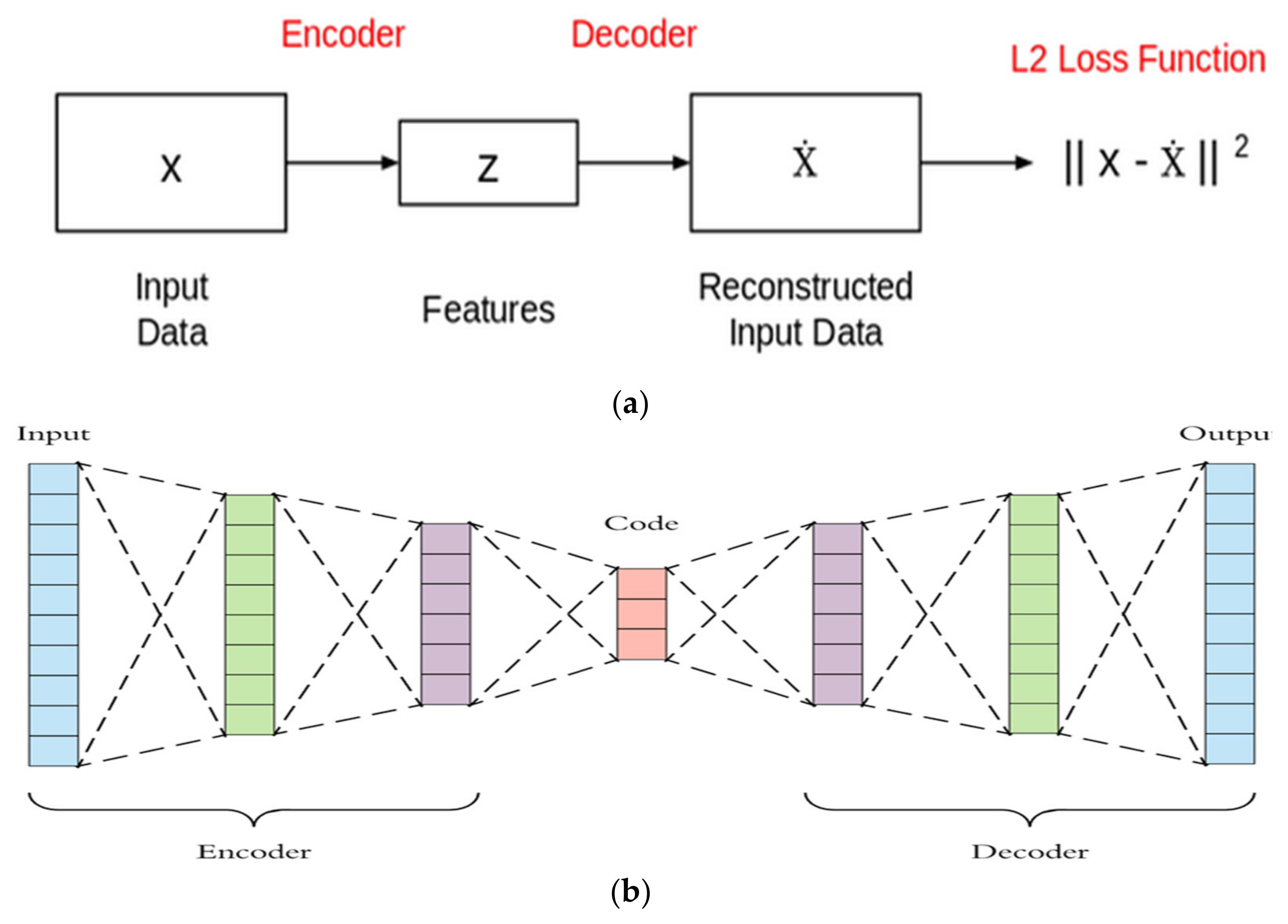
The autoencoder consists of two parts: an encoder and a decoder. The encoder takes the input (X) and extracts features/code (z) from it with the help of convolution and maxpooling layers, and then, these features are used by the decoder to reconstruct the input (output X^) from those features as shown in Figure 9a,b.

Figure 9. (a) Simplified autoencoder model. (b) Visual representation of autoencoder architecture.

The loss is then calculated between the input (X) and output (X^), and the loss calculated in most cases is usually MSE (mean squared error). MSE was used, as it seems simple to implement, and model training is quiet and fast for using this loss in this complicated architecture. If the output (X^) is different from the input (X), the loss penalizes it and helps to reconstruct the input data. A small tweak was performed in the convolutional autoencoder. Instead of calculating the loss between the input image and the reconstructed image, the loss is calculated by comparing the ground truth image and the reconstructed image as shown in Figure 10. By doing so, the resultant image is better in terms of quality and reduced noise.

Figure 10. Visual representation of autoencoder model.

The conventional autoencoder as trained in this way on all the low-resolution images in the dataset, and the reconstructed images were then passed to the CNN based on ResNet Architecture. ResNet architecture is well suited for images and also performs well in these cases. Due to the skip connections, the model parameters are far less, and also the training is quite fast.

The image passes through a number of convolutional layers, and various operations are performed on the image at a different stage of the network, such as maxpooling, which is a sample-based discretization process and extracts features, such as sharp and smooth edges. Batch normalization is another operation for achieving higher learning rates in the network. ReLu is yet another operation for activation, which helps in vanishing gradient problems while learning. Various other operations resulting in better learning of the model through training and in creating higher resolution images from the reconstructed image output from the autoencoder are shown in Figure 11.

Figure 11. Visual representation of ResNet-based CNN model.

4.5. Computational Overhead of the Proposed Model

Considering an input image I(x,y) of size n×n and a patch W of a size equivalent to the size of the filter, suppose a filter g(x,y) is of size f1 × f1 (i.e., 7 × 7, 5 × 5 and 3 × 3). The convolution of the input image with the filter may be defined as P = I(x,y)*g(x,y). The total number of the operations during a convolution operation will result in a response feature map of size P (i.e., |P|=(n × n)/W). Taking the number of channels for our model as C, the response of a convolution operation will be P × C. The total computational overhead for our proposed model may be computed by taking into consideration of the layer-wise number of filters used successively. For the proposed method, computation overhead equals O(64 × P × C + 128 × P × C + 256 × P × C + 512 × P × C). Therefore, the computational complexity of the model can be given as an order of O(PC).

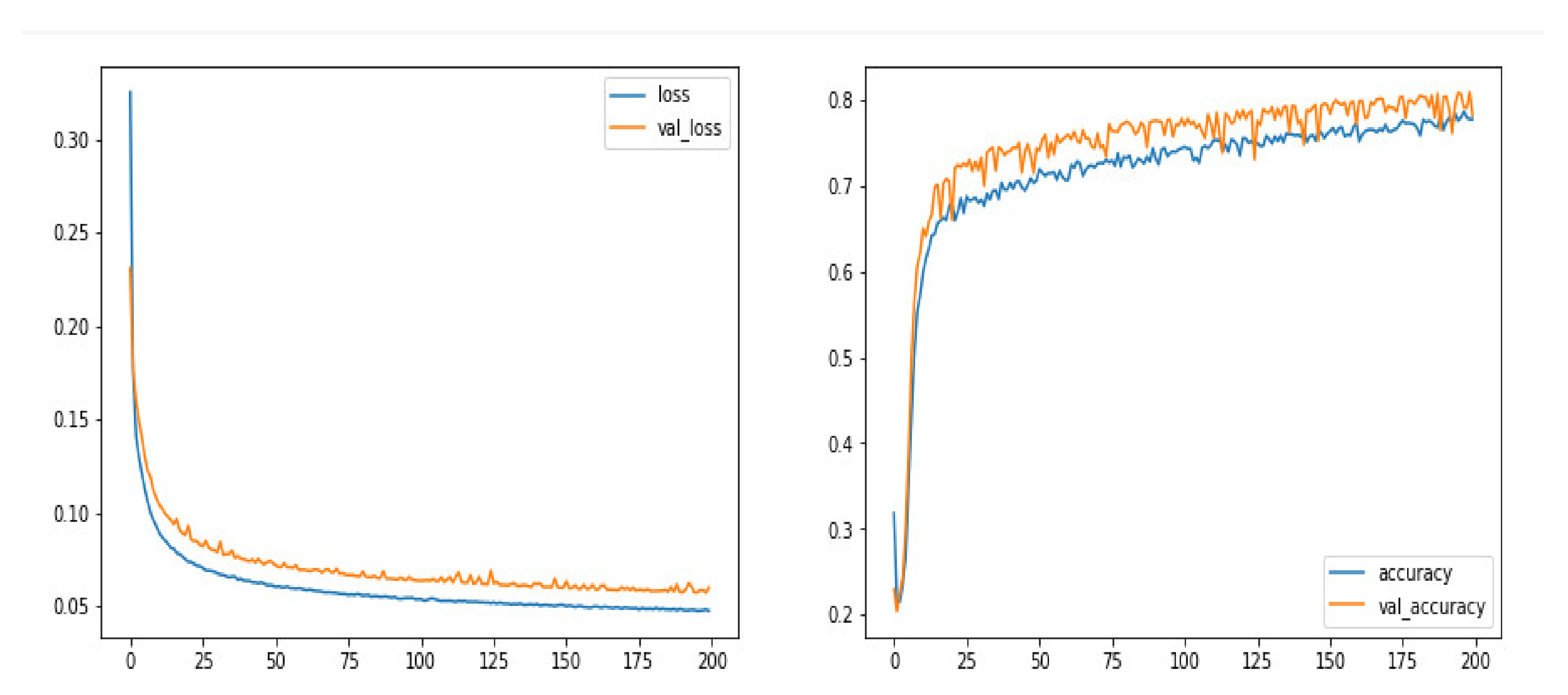
4.6. Visualizing the Losses and Accuracies

Since MSE loss function has been used for training purposes, accuracies and losses were visualized in order to predict the problems and model-related changes in the architecture. Separate functions were written for this purpose, and different libraries were used for plotting the losses and accuracies. In the next section, we explore the experiments performed on the proposed model and the obtained from them.

5. Experiments and Results

Various experiments were performed on the model itself, and it was also trained on different datasets. Moreover, the effect of the model and data on accuracies and losses were also visualized. Following datasets have been used in this study.

5.1. Experiment 1—LFW (Labelled Faces in the Wild) Dataset

This dataset [29] contained face images and is usually used for studying unconstrained face recognition, but it was used to train our model in order to see how our model would learn about-face and how well it would be able to perform the task of super-resolution on it.

Firstly, convolutional autoencoders was trained to check its performance and understand how well it would be able to learn and reconstruct images. The images given to this model were 80 × 80 in terms of their resolution.

The model summary of the convolutional autoencoder is given in Figure 12.

Figure 12. Model Summary of Convolutional Autoencoder.

Accuracy of around 93% (validation accuracy) and a loss of around 0.0025 (validation loss as compared to 0.0028 loss) was observed after training it on this dataset. The input (80 × 80) and the model predictions of this model are given in Figure 13. Furthermore, this model was trained on input images of resolution 80 × 80.

Figure 13. Convolutional Autoencoder Input and Prediction (LFW Dataset).

5.2. Experiment 2

Another dataset was used on this model, which contained around 100 lower- and higher-resolution images obtained from various sources, but it showed similar results as on the previous dataset. Thus, changes were made to the model by increasing the number of convolutional neural network layers and modifying various parameters in the model. The modified convolutional autoencoder model summary is given in Figure 14.

Figure 14. Modified Convolutional Autoencoder.

5.3. Experiment 3

This model was trained on a dataset containing 855 high- and low-resolution images each. The model showed a validation accuracy of around 88% and a validation loss of around 0.05 while training the network on 200 epochs (iterations). Figure 15 shows the plots between loss and validation loss and between accuracy and validation accuracy. Figure 16 shows the input, prediction of the model, and the ground truth image.

Figure 15. Plot of various parameters obtained from training and validation.

Figure 16. Input, Predicted, and Ground truth images.

5.4. Experiment 4

The output of the predicted images from the convolutional autoencoder were saved and added to the dataset to process them further and create a super-resolution image with the help of ResNet-based CNN. The predicted images were given the ResNet-based architecture with their ground truth and other lower-resolution images. The model was trained on them to achieve a higher SSIM (structural similarity) concerning ground and high PSNR (peak signal-to-noise ratio) than the reconstructed images obtained from convolutional autoencoder. The ResNet-based CNN model used here consists of 10 residual blocks and various other convolutional network layers, which make a total of 100+ layers. Figure 17 shows the plot of SSIM, PSNR, and the loss of the model obtained while training and validating it.

Figure 17. PSNR, SSIM, and Loss of ResNet-based CNN model.

From the plots, it can be predicted that by increasing the number the epochs, we might be able to increase the PSNR and SSIM, as the plots show an increase with each epoch, which is the main aim of this proposed model. The model was able to attain an SSIM of 92% and a PSNR of around 25 dB on average during training and validation.

Figure 18 shows the input, predicted image, and the ground truth (high-resolution) image.

Figure 18. Input, Prediction, and Ground truth (high-resolution) image of ResNet-based CNN.

From the predictions of this models, it can be concluded that our proposed work performs well in terms of performing super-resolution on low-resolution images.

6. Comparison with Different State of the Art (SOTA) Approaches

Table 1 illustrates PSNR and SSIM of our proposed work and different state-of-the-art approaches.

Table 1. PSNR and SSIM comparison.

Model	PSNR (db)	SSIM
NDL [30]	19.74	89
DDL [30]	23.01	95
Our model	25.00	92

Our proposed method clearly performs better in comparison to the other models. Figure 19 shows the box and whisker plot, which is based on the data of Table 1.

Figure 19. PSNR and SSIM comparison.

7. Conclusions and Future Work

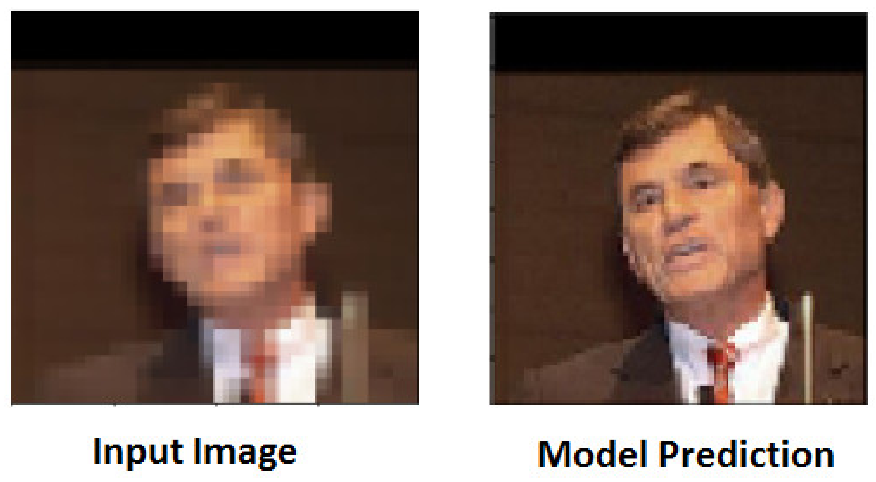
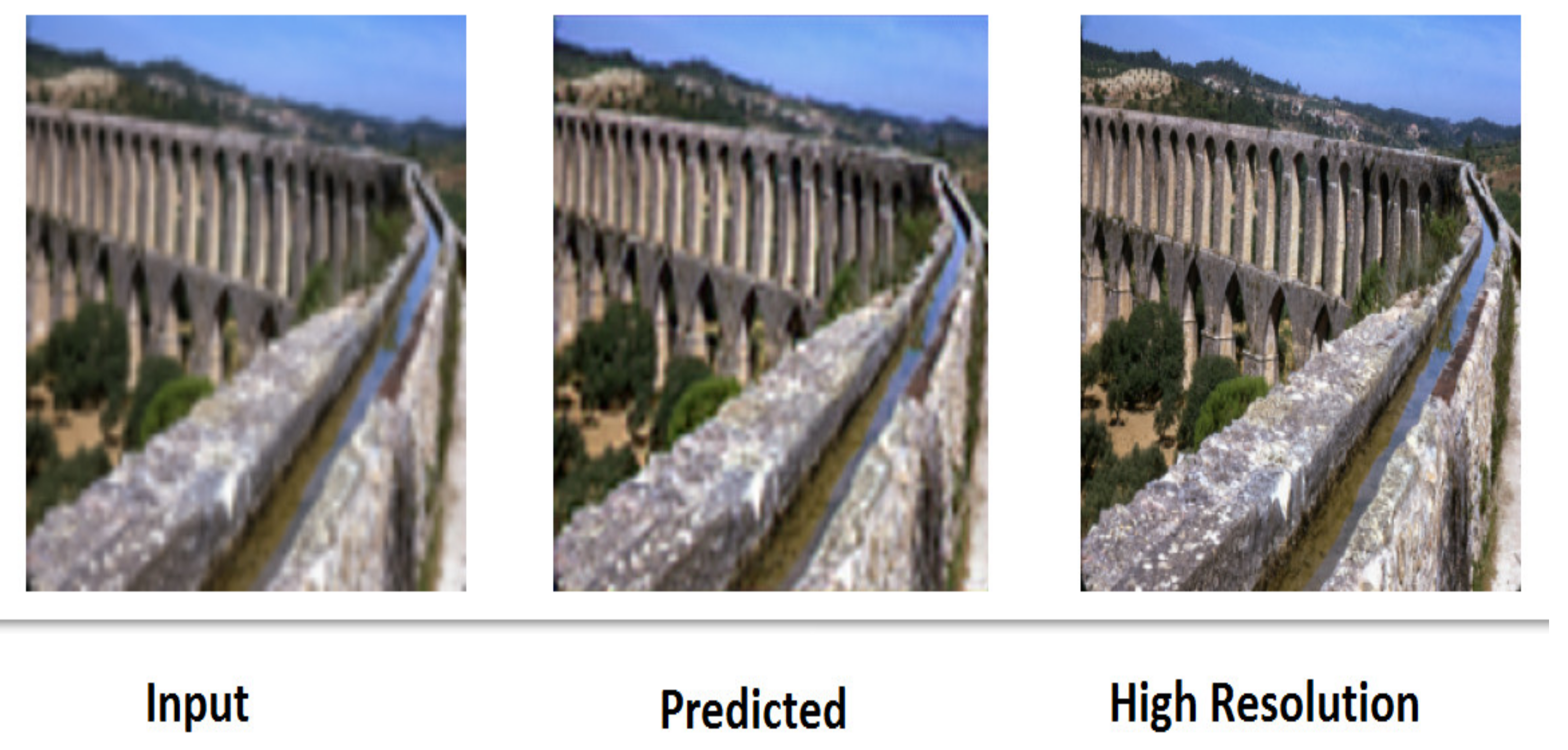
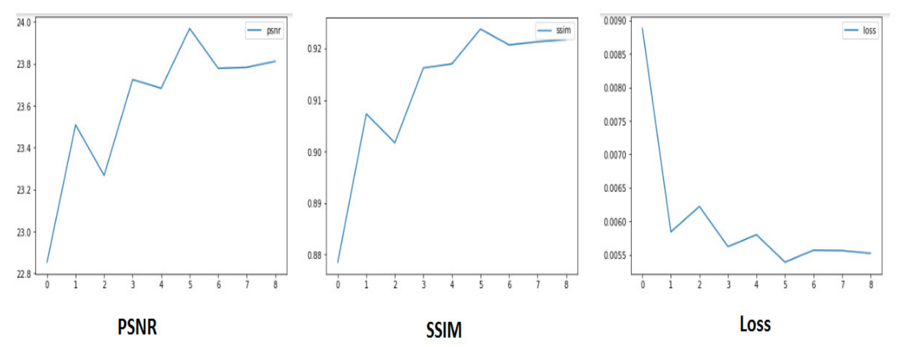
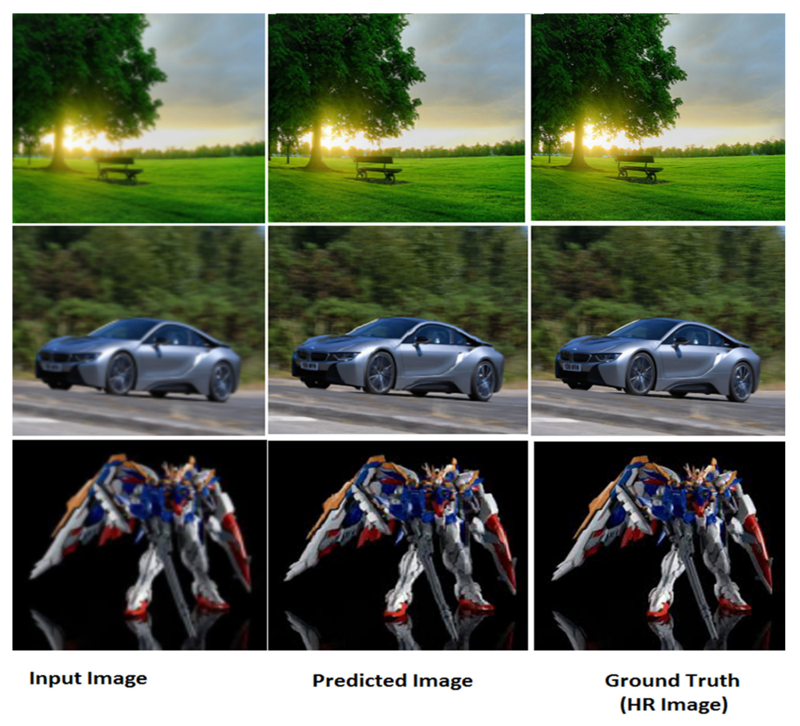
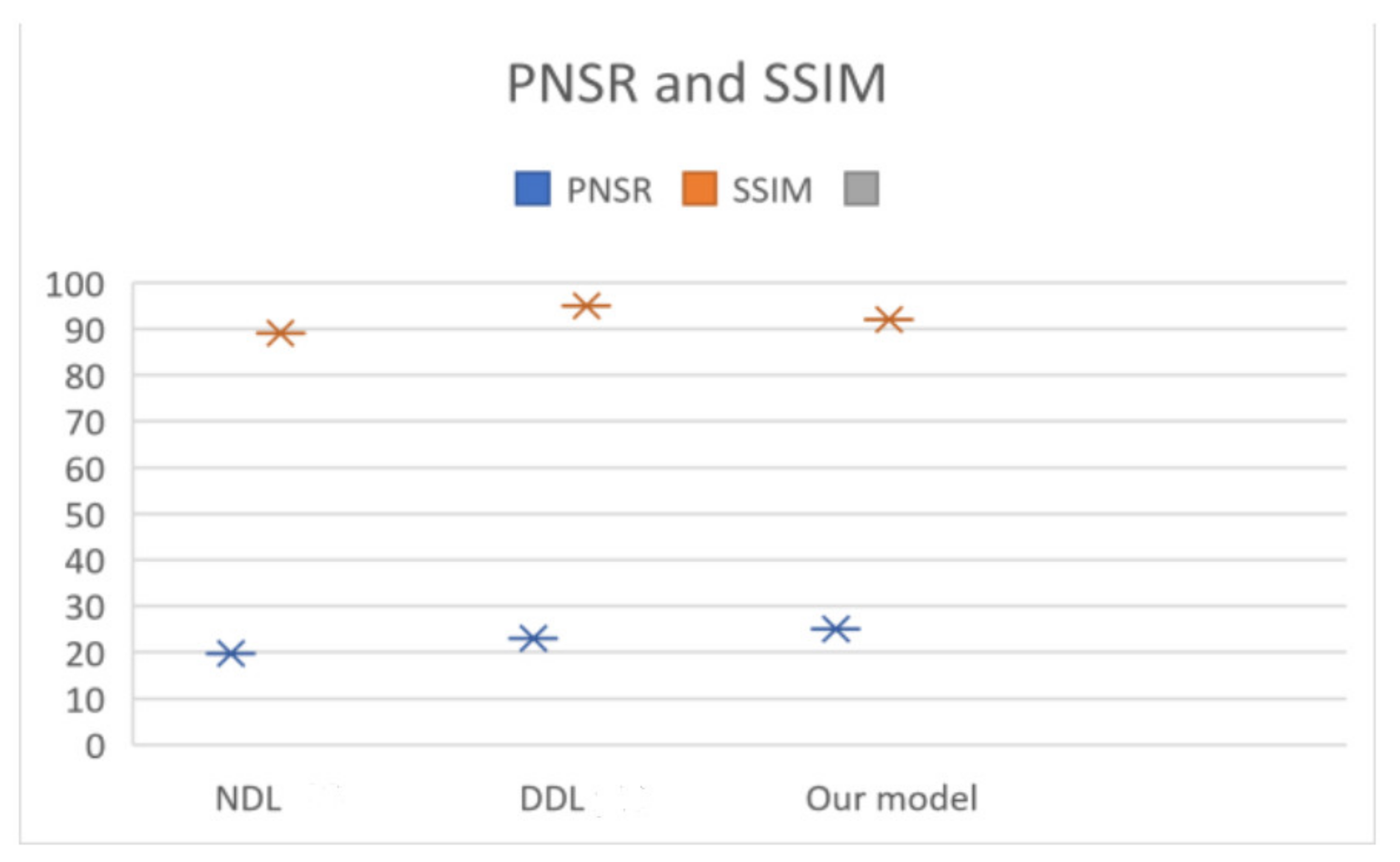
Image super-resolution has been one of the most studied topics in the image-processing area. Especially, single-image super-resolution is the most focused branch of super image resolution. Obtaining a high-resolution image by using only one single input image is an outstanding and efficient idea for many reasons, such as the disability of taking multiple images or affordability. For example, MRI is an expensive imaging technique. Performing it multiple times costs a great deal. Therefore, the concept of single-image super-resolution is a very efficient way to overcome these types of issues. In this paper, a single-image super-resolution network based on two state-of-the-art methods, autoencoders and Deep Residual Networks, has been proposed. In the model, we also applied the different pre-processing procedures to obtain a better PSNR/SSIM performance. The experimental results illustrate that the proposed method shows outstanding performance regarding image quantitative and visual comparison. Thus, the proposed method generates clear and better-detailed output HR images. How to use CNN to improve the quality and resolution of any image has been successfully demonstrated. However, numerous challenges were encountered in terms of time complexity, resource utilization, and optimization during this study.

Future work can improve on this study by employing more sophisticated models derived from CNN that can reduce model generation computation time and by employing algorithms that can reduce resource usage (GPU). Additionally, improvements can be made to how this system processes each image to create a higher-resolution (super-resolution) version of that image. Furthermore, there can be more than one way to perform such actions, and by combining more methods, greater perfection in our model can be achieved.

This model has very large capabilities, but due to GPU limitations (as it requires a great deal of resources), we had to compromise in terms of (training time) by limiting the training iterations during the training of this model. Accordingly, there is much room for improvement if the proper resources are allotted to generate a better super-resolution of an image. Finally, additional enhancements that can be made to this model include support for a wide range of image formats, allowing this model to be universally accepted. Further to improve results’ visualization, box and whiskers diagrams can be drawn to show the solutions’ dispersity over multiple runs. A confusion matrix can be made to provide better insights into obtained performance