Effect of Slow–Fast Time Scale on Transient Dynamics in a Realistic Prey-Predator System

Abstract

Systems with multiple time scales, often referred to as `slow–fast systems’, have been a focus of research for about three decades. Such systems show a variety of interesting, sometimes counter-intuitive dynamical behaviors and are believed to, in many cases, provide a more realistic description of ecological dynamics. In particular, the presence of slow–fast time scales is known to be one of the main mechanisms resulting in long transients—dynamical behavior that mimics a system’s asymptotic regime but only lasts for a finite (albeit very long) time. A prey–predator system where the prey growth rate is much larger than that of the predator is a paradigmatic example of slow–fast systems. In this paper, we provide detailed investigation of a more advanced variant of prey–predator system that has been overlooked in previous studies, that is, where the predator response is ratio-dependent and the predator mortality is nonlinear. We perform a comprehensive analytical study of this system to reveal a sequence of bifurcations that are responsible for the change in the system dynamics from a simple steady state and/or a limit cycle to canards and relaxation oscillations. We then consider how those changes in the system dynamics affect the properties of long transient dynamics. We conclude with a discussion of the ecological implications of our findings, in particular to argue that the changes in the system dynamics in response to an increase of the time scale ratio are counter-intuitive or even paradoxical.

1. Introduction

The study of population dynamics of the interacting species in an ecosystem plays an important role in understanding the survival and long term existence of various species. Therefore, comprehending the intricate dynamics of the system through mathematically tractable yet realistic models are necessary. In this regard, presence of multiple time scales due to the difference in growth rates when measured with respect to a fixed time scale plays a crucial role. The interacting species often evolve in different time scales, and incorporating them explicitly in the mathematical models can significantly alter the dynamics of the model and capture some realistic scenarios. Prey–predator models are building blocks of several long food chains and food-webs. Assuming that the rate of growth of prey population is much faster than its predator, we define the time scale parameter $\epsilon$ as the ratio of the time scales at which prey and predator evolves. The prey–predator models with a small time scale parameter $\epsilon (0<\epsilon \ll 1)$ can be characterized as a singularly perturbed differential equation, with $\epsilon$ being the singular parameter. These types of systems were initially observed in many chemical systems where the reaction rates of the reactants differs widely. However, in the context of ecology, this has been gaining attention over the last two decades. Rinaldi and Muratori first studied the slow–fast prey predator models where the cyclic existence of the slow–fast limit cycle was discussed [1,2]. They also analyzed the cyclical fluctuation in population densities of three species model in a slow–fast setting with one and multiple time scale parameter.

The slow–fast systems are analyzed with the help of various mathematical tools. In 1970, Neil Fenichel developed a geometric technique [3] with the help of invariant manifold theory to study this class of systems. The basic idea was to reduce the full system into lower dimensional sub-systems which are easier to work with. In this way, the dynamics of the full system can be analyzed by concatenating the dynamics of each sub-systems. Later, the authors in [4,5] extended this theory and explained the role of non-hyperbolic points such as fold and canard points on the resulting dynamics. These theories were applied by the researchers to study the dynamics of prey–predator models with prey-dependent functional response. In [6], the authors have considered the classical classical Rosenzweig–MacArthur (RM) model and the Mass Balance chemostat model. In [7], the authors have shown the role of multiplicative Allee effect multiplicative on the slow–fast dynamics with prey-dependent functional response. It is evident that the predator dependent functional responses can depict the species interaction more precisely.

Apart from the existence of steady state and Hopf bifurcating limit cycles, the slow–fast systems can exhibit much more complex asymptotic dynamics, known as canard cycles and relaxation oscillations. These cycles are peculiar for the singularly perturbed systems. In the long term, one complete cycle can include many generations of prey and predator which includes sudden outbreak or slow decline in population densities. These transitions from one state to another can be best understood if we study the system over a shorter time scale. Therefore, apart from asymptotic dynamics, there has been growing interest among the researchers to understand the transient dynamics in ecological systems [8,9]. More realistically, due to several environmental factors, the system might take longer time to settle down to any attractor, and in that scenario the study of transient dynamics can be more relevant. Recently, it gave new direction in understanding the major factors behind regime shift which is associated with a catastrophic change in the ecosystem. Characterizing and identifying the pattern in the transient can be used to predict possible drastic changes in the population dynamics. The duration of the transients are sometime long enough to be mistakenly depicted as asymptotic dynamics of the system, known as long transients. Various factors are involved in understanding long transients, including system properties, the background bifurcation parameter, the initial state of the system, etc., e.g., see [10,11,12] for details.

The main objective of this work is to study both short-term and long-term dynamics of a prey–predator model. We consider a slow–fast predator–prey model with ratio-dependent functional response and intra-specific competition among the predators. With the help of extensive numerical simulations, we give a complete bifurcation structure of the model. We also study the slow–fast attractors of the system, namely canard cycles and relaxation oscillation, and obtain the parametric regimes for the existence and non-existence of such solutions. We further study the different transient dynamics observed in the system and the effect of the time scale parameter in altering the nature and duration of the transient.

The article is organized as follows. In Section 2, we introduce the slow–fast model and some basic properties of the model. Section 3 deals with the complete bifurcation analysis of the model for $\epsilon =1$ and also for $0<\epsilon <1$, followed by the slow–fast nature of the attractors in Section 4. Here, we discuss the existence and non-existence of the relaxation oscillations and canard cycles. In Section 5, with the help of numerical simulations, we show different transient dynamics exhibited by the model, and discuss the effects of various background parameters on the nature and duration of the transient.

2. The Slow–Fast Model

We consider a two species predator–prey model with ratio-dependent functional response and density dependent death rate of the predator as

$$\begin{array}{cc}\hfill & \frac{du}{dt}=u-u^2-\frac{\alpha uv}{u+v}:=f(u,v),\hfill \\ \hfill & \frac{dv}{dt}=\epsilon \left(\frac{\beta uv}{u+v}-\gamma v-\delta v^2\right):=\epsilon g(u,v),\hfill \end{array}$$

(1)

where the dimensionless variables u and v are prey and predator density, respectively, at time t, and $0<\epsilon \ll 1$ is the time scale parameter [13,14,15,16]. The solution of (1) is composed of the slow and fast motions for $(\epsilon <1$), which are obtained by decomposing the above system into fast and slow subsystems, respectively, as follows

$$\begin{array}{cc}\hfill & \frac{du}{dt}=f(u,v),\hfill \\ \hfill & \frac{dv}{dt}=0,\hfill \end{array}$$

(2)

$$\begin{array}{cc}\hfill & 0=f(u,v),\hfill \\ \hfill & \frac{dv}{d\tau }=g(u,v),\hfill \end{array}$$

(3)

where $\tau$ is the slow time, t is the fast time, and $\tau =\epsilon t$, $0<\epsilon <1$. The subsystems (2) and (3) are known as fast subsystem and slow subsystem, respectively.

The non-trival equilibria of the fast subsystem forms the non-trivial critical manifold $C_0=\left\{(u,v)\in {\mathbb{R}}_{+}^2:v=q\left(u\right):=\frac{u(1-u)}{u+\alpha -1},0<u<1,v\ge 0\right\}$. The maxima of $C_0$ denotes the fold of the critical manifold, which is given by

$$u_f=-\alpha +1+\sqrt{\alpha (\alpha -1)},v_f=\frac{u_f(1-u_f)}{u_f+\alpha -1},\alpha >1.$$

This fold point divides the critical manifold $C_0$ into normally hyperbolic, attracting $C_0^a$ and repelling sub-manifold $C_0^r$. The model can have at most two coexisting equilibrium, depending on the position of the nullclines. For $\alpha >1$, the non-trivial prey nullcline is increasing for $0<u<u_f$ and decreasing for $u_f<u\le 1.$ Whereas, for $\alpha <1$, the nullcline is monotonically decreasing. Throughout this paper we will consider $\alpha =2$ and $\gamma =0.6.$ The authors in [16] described in detail different parametric regimes for the existence of one, two, or no equilibrium points. Here, we explore those regimes and study the shift in the parametric regimes due to the influence of the time scale parameter $0<\epsilon \ll 1.$ Defining the system at origin as $f(0,0)=0=g(0,0)$, we obtain that $E_0=(0,0)$ is an equilibrium point of the system. The axial equilibrium point $E_1=(1,0)$ is always a saddle point. Under the parametric restriction, as discussed in [16], $\alpha >1,\beta >\gamma$, $E_{1*}$, and $E_{2*}$ are the two interior equilibrium points of the system which are given by

$$u_{j*}=\frac{T\pm \sqrt{D}}{2(\alpha \delta +\beta )},\mathrm{and}{v}_{j*}=\frac{u_{j*}(1-u_{j*})}{u_{j*}+\alpha -1},j=1,2$$

where $T=\alpha \gamma -2\alpha \beta +\alpha \delta +2\beta$ and $D={\alpha }^2{\gamma }^2-2{\alpha }^2\gamma \delta +4{\alpha }^2\beta \delta +{\alpha }^2{\delta }^2+4{\alpha }^3\delta (\gamma -\beta ).$ These two equilibrium points collide at $\beta ={\beta }_{SN}$ to produce an unique equilibrium point $E_{SN}(u_{SN},v_{SN})$ whose components are

$$u_{SN}=\frac{\alpha \gamma -2\alpha \beta +\alpha \delta +2\delta }{2(\alpha \delta +\beta )},v_{SN}=\frac{u_{SN}(1-u_{SN})}{u_{SN}+\alpha -1},$$

where $T>0,\alpha >1$, and $u_{SN}<1.$

3. Bifurcation Results

The system (1) can have either two equilibrium points or no equilibrium point for $\beta >{\beta }_{SN}.$ Whenever it has two interior equilibrium points, say $E_{1*}=(u_{1*},v_{1*})$ and $E_{2*}=(u_{2*},v_{2*})$, such that $u_{1*}<u_{2*},$ then from linear stability analysis $E_{1*}$ is always a saddle point and $E_{2*}$ can either be stable or unstable. These two interior equilibrium points collide and disappear via saddle node bifurcation along the magenta curve in Figure 1, below which the system does not have any interior equilibrium. For $\beta <{\beta }_{SN},$ the system has a unique interior equilibrium $E_{*}$. We linearize the system (1) near $E_{*}$ and the Jacobian matrix evaluated at $E_{*}$ is given by

$$J_{*}=\left(\begin{array}{cc}1-2u_{*}-\frac{\alpha u_{*}^2}{{(u_{*}+v_{*})}^2}& -\frac{\alpha u_{*}^2}{{(u_{*}+v_{*})}^2}\\ \frac{\epsilon \beta v_{*}^2}{{(u_{*}+v_{*})}^2}& \epsilon \left(\frac{\beta u_{*}^2}{{(u_{*}+v_{*})}^2}-g-2\delta v_{*}\right)\end{array}\right).$$

(4)

Figure 1. Two parametric global bifurcation diagram of system (1) for $\alpha =2,\gamma =0.6,$ and $\epsilon =1$. ${\beta }_{GH},{\beta }_{TC},and{\beta }_{HT}$ represent the $\beta$-threshold for generalized Hopf bifurcation, transcritical bifurcation, and Bogdanov–Takens bifurcation, respectively. The point CP is the cusp point, the intersection of the vertical line ${\beta }_{TC}$ with the saddle node bifurcation curve of equilibrium points.

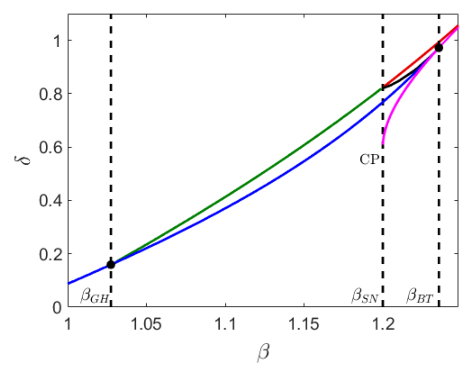
The interior equilibrium point $E_{*}$ (when $\beta <{\beta }_{SN}$) or the interior equilibrium $E_{2*}$ (when $\beta >{\beta }_{SN}$) loses its stability through Hopf bifurcation. The model without any time scale difference, that is for $\epsilon =1$, is well studied in literature [16,17] where the authors analytically considered the broad variety of bifurcation that the model exhibits. A complete two parametric bifurcation diagram is shown in Figure 1 where the blue curve represents the Hopf bifurcation curve. Along the Hopf bifurcation curve there exists a co-dimension two bifurcation point known as the Bogdanov–Takens bifurcation point [18], where the saddle node and bifurcation curve intersect. The Hopf bifurcation can be either supercritical or subcritical, depending on whether the first Lyapunov number is negative or positive. The change in the Hopf bifurcation from supercritical to subcritical takes place at the generalized Hopf bifurcation threshold (GH), where the first Lyapunov number is zero. The Hopf bifurcation is supercritical for $\beta <{\beta }_{GH}$ and subcritical for $\beta >{\beta }_{GH}.$ Small stable limit cycles exist for $\beta <{\beta }_{GH}$ and parameter values taken below the Hopf bifurcation curve. Because of the complexity of the algebraic equation, we cannot explicitly find the Hopf threshold from Trace $\left(J_{*}\right)=0.$ However, the Hopf bifurcation threshold depends on $\epsilon ,$ and thus by varying $\epsilon$, the stability regime of the interior equilibrium point shifts. For instance, keeping the parameter values fixed at $\alpha =2,\gamma =0.6,\beta =1.001$, for $\epsilon =1$ the Hopf threshold ${\delta }_H=0.09,$ whereas for $\epsilon =0.1,{\delta }_H=0.57.$ The green curve represents the saddle-node bifurcation of limit cycles which exists for ${\beta }_{GH}<\beta <{\beta }_{SN}$, and it intersects with a global bifurcation curve (red) and a homoclinic bifurcation curve (black) at $\beta ={\beta }_{SN}.$ For a fixed $\beta$, as we decrease $\delta$ from the saddle node bifurcation curve, two limit cycles are born. The outer stable cycle coexists with the inner unstable cycle in a small parametric domain enclosed by the saddle node bifurcation of limit cycles and the Hopf bifurcation curve. The unstable limit cycle disappears via subcritical Hopf bifurcation and the interior equilibrium becomes unstable. In the region below the blue curve, the stable cycle coexists with an unstable equilibrium point.

In the region enclosed by the red and black curve, a stable cycle is formed whenever the unstable manifold of the axial equilibrium $E_1$ collides with the stable and unstable manifold of the $E_0.$ The stable limit cycle itself acts as a separatrix between the stable equilibrium and the stable cycle. For a fixed $\beta ,$ such that ${\beta }_{SN}<\beta <{\beta }_{BT}$, if we move down from the red curve, the stable cycle and the stable equilibrium coexist in a very narrow domain until the homoclinic bifurcation curve (black). At this point, an unstable limit cycle is created surrounding the stable interior equilibrium. In the domain enclosed by the homoclinic and Hopf bifurcation curve and ${\beta }_{TC}$, we observe a stable interior equilibrum, surrounded by an unstable limit cycle which again is surrounded by a stable limit cycle. Further decreasing $\delta$, the unstable cycle disappears via subcritical Hopf bifurcation (blue) and the stable cycle persists.

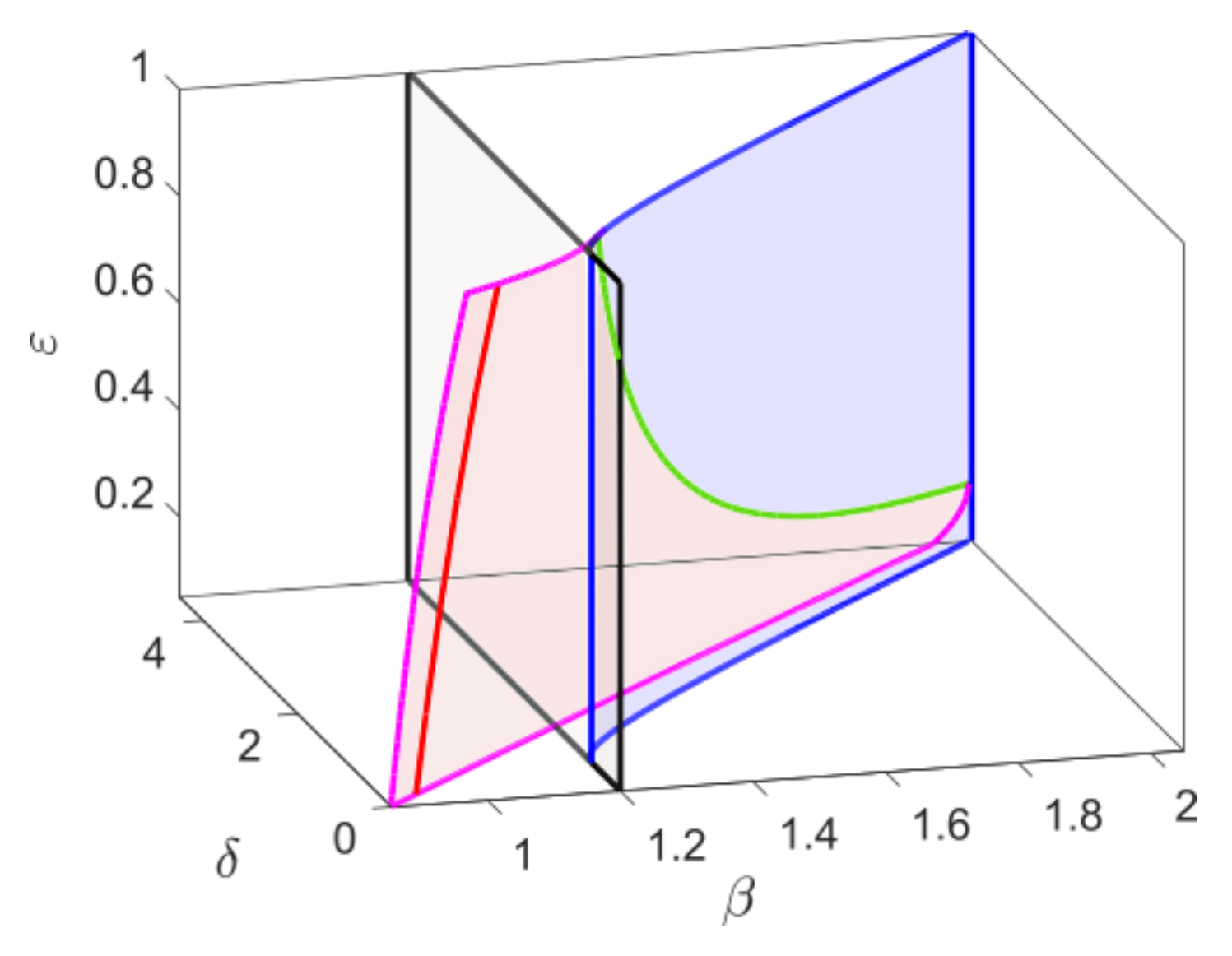
We finally show the effect of the time scale parameter on the bifurcation thresholds of the system. The parameter $\epsilon$ has no effect on the components of the equilibrium points, the saddle node bifurcation, and transcritical bifurcation is independent of $\epsilon .$ However, the Hopf bifurcation threshold changes for $\epsilon <1$ and thus the GH and BT point. Figure 2 shows the bifurcation structure of the system while considering $\epsilon$ as a third parameter along with $\beta$ and $\delta$. The saddle-node bifurcation surface is bounded by the blue curves, which intersect with the Hopf bifurcation surface (pink) along the BT-bifurcation curve (green). In the Hopf bifurcation surface, the generalized Hopf curve is plotted in red and the gray surface represents the transcritical bifurcation surface which intersects with the saddle node bifurcation surface along the CP curve (blue). Varying $\epsilon$, the Hopf bifurcation threshold shifts, but the saddle-node bifurcation threshold remains fixed. Therefore, the BT-bifurcation threshold shifts and for sufficiently small values of $\epsilon (<0.05)$, the Hopf and saddle node curve almost becomes parallel and BT threshold cease to exist. Using mathematical techniques previously developed to study system’s bifurcation structure [18,19] and with the help of simulations done with MATLAB, we obtained the bifurcation diagrams presented in this section.

Figure 2. Three dimensional bifurcation diagram of the system (1) with the time scale parameter $\epsilon$ in the vertical axis. The parameters $\alpha$ and $\gamma$ are same as in Figure 1. The curves and each surfaces are explained in the text.

4. Slow–Fast Dynamics

In this section we consider slow–fast dynamics of the system (1) depending on the position of the interior equilibrium point(s) with respect to the fold point. The fold point divides the critical manifold $C_0$ into attracting and repelling sub-manifolds. First, we consider the case when the system has a unique equilibrium point.

Lemma 1.

Assume that the system (1) has a unique equilibrium point. Then for ε sufficiently small the Hopf bifurcation point converges to the fold point.

Proof. 

The Jacobian matrix evaluated at the interior equilibrium point $E_{*}(u_{*},v_{*})$ is given as

$$J=\left(\begin{array}{cc}{f}_u(u_{*},v_{*})& g_u(u_{*},v_{*})\\ \epsilon g_u(u_{*},v_{*})& \epsilon g_v(u_{*},v_{*})\end{array}\right).$$

(5)

The Hopf bifurcation threshold is obtained from the equation Trace $\left(J\right)=0$, which gives $f_u(u_{*},v_{*})+\epsilon g_v(u_{*},v_{*})=0.$ For $\epsilon =1$, both $f_u$ and $g_v$ contribute in obtaining the Hopf threshold as $g_v(u_{*},v_{*})\ne 0$ for predator dependent functional response. However, for $\epsilon \to 0,$ the condition for Hopf bifurcation reduces to $f_u(u_{*},v_{*})\to 0,$ which is precisely the condition for obtaining the fold point. Thus, as $\epsilon \to 0,$ the Hopf bifurcation point converges to the fold point. □

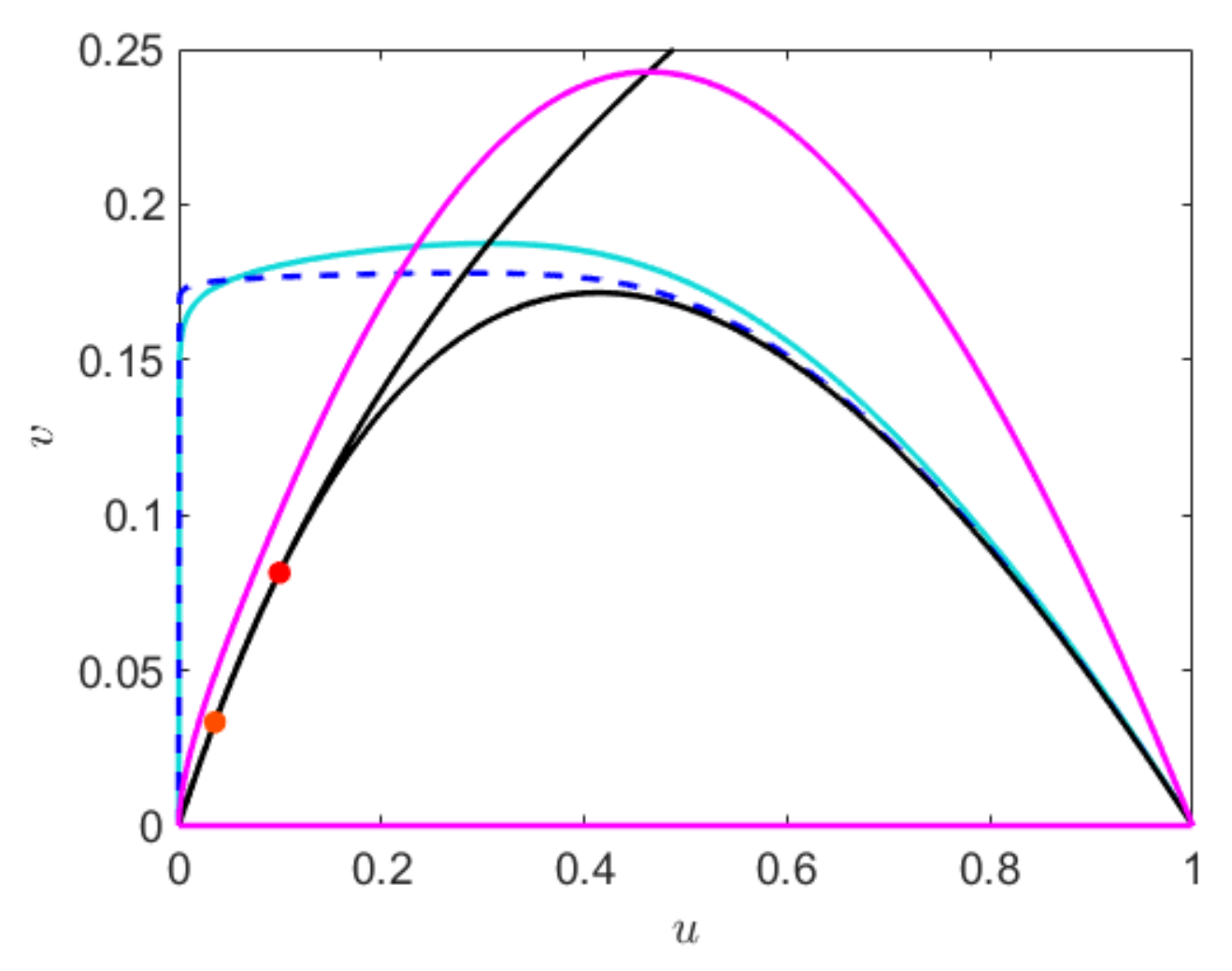
Whenever the non-trivial predator nullcline intersects with the non-trivial prey nullcline at the fold point, the small amplitude Hopf bifurcating limit cycle transforms to large amplitude relaxation oscillation through a family of canard cycles. In this case, the fold point is the canard point by Lemma 1 and the periodic orbit after following the vicinity of the attracting sub-manifold $C_0^a$ until the fold point $(u_f,v_f)$, then following the repelling sub-manifold $C_0^r$ for a considerable time before jumping to the trivial critical manifold $u=0$ forming canard cycle. (For details, please refer to the Section 4 of [7]). This transition takes place in a narrow parameter range, giving rise to canard explosion. In this case, the canard cycles are formed in the vicinity of super-critical Hopf bifurcation and are stable in nature. Taking $\beta =0.88,\epsilon =0.05$, the canard cycle (with and without head) and the relaxation oscillation is shown in Figure 3a. We find a small canard cycle for $\delta =0.111\left(\mathrm{green}\right),$ a canard cycle with head for $\delta =0.1104\left(\mathrm{magenta}\right)$ and relaxation oscillation for $\delta =0.09\left(\mathrm{blue}\right)$. The change in the amplitude of the limit cycle in the narrow domain of $\delta$ is shown in Figure 3b, which gives rise to canard explosion.

Figure 3. (a) Canard cycle without head (green) for $\delta =0.111,$ canard cycle with head for $\delta =0.1104,$ relaxation oscillation for $\delta =0.09.$ (b) The bifurcation diagram the change in the amplitude of the limit cycle. Canard explosion occurs in the pink shaded region. The other parameter values are fixed at $\alpha =2,\gamma =0.6,\beta =0.88$, and $\epsilon =0.05.$.

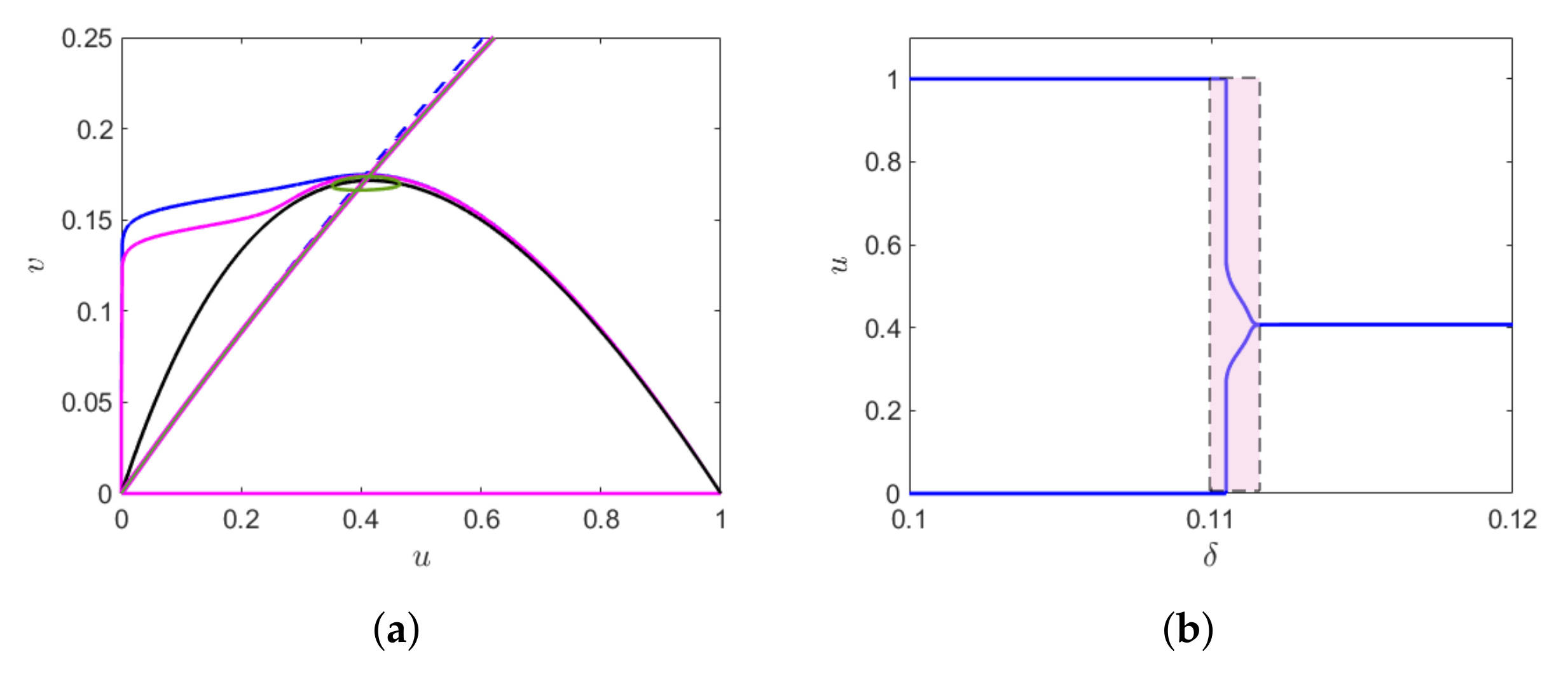
We now consider the case when the Hopf bifurcation is sub-critical. From Theorem 8.4.3 of [20], it follows that since the sub-critical Hopf lies at $O\left(\epsilon \right)$ distance from the fold point, there exists a unique value of $\delta$ at which the canard cycles undergoes a saddle node bifurcation of limit cycles. The results are sketched in Figure 4. For $\beta =1.15$ and $\epsilon =0.1$, the sub-critical Hopf bifurcation occurs at ${\delta }_H=1.142.$ The small amplitude canard cycle is unstable surrounded by a stable cycle and the saddle node bifurcation of limit cycles occurs at $\delta =1.158.$ The canard explosion occurs within the shaded region (gray), that is, between the thresholds of sub-critical Hopf bifurcation and the saddle node bifurcation of limit cycles.

Figure 4. (a) Stable canard cycle with head (blue) and unstable canard cycle (red) for $\beta =1.15,\delta =0.158$, and $\epsilon =0.1.$ Green dot represents stable equilibrium point. (b) The bifurcation diagram shows the change in the amplitude of v-component of the limit cycle. The solid line represents the maximum and minimum amplitude of limit cycles, stable (blue), and unstable (red). The broken line shows the unique interior component where red represents unstable and blue is for stable.

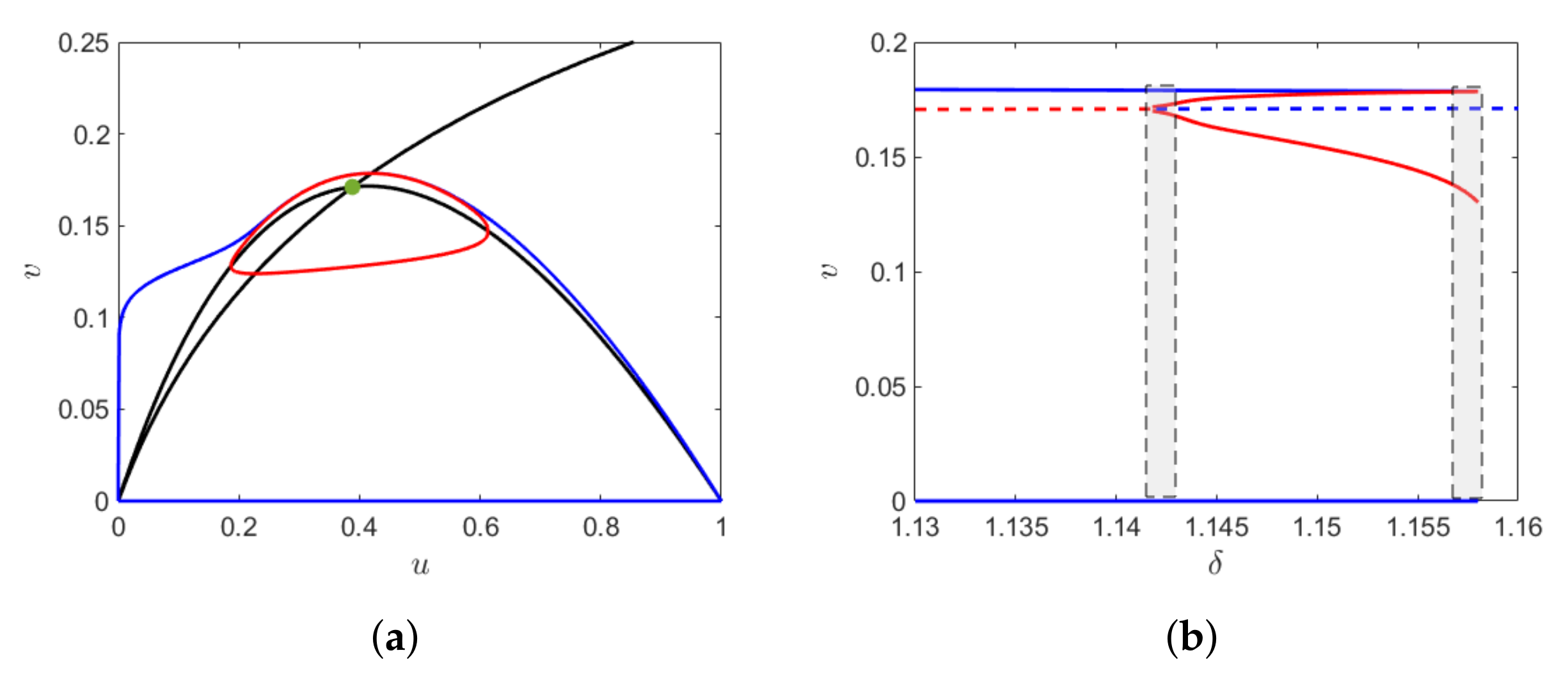
We then consider a parametric domain where the system has two equilibrium points, say $E_{1*}(u_{1*},v_{1*})$ and $E_{2*}(u_{2*},v_{2*})$, such that $0<u_{1*}<u_{2*}<u_f,$ where $u_f$ is the $u-$ component of the fold point. Then for $0<\epsilon \ll 1$ we have the following result.

Theorem 1.

Let ${\gamma }_0$ be the singular trajectory consists of concatenated alternate fast and slow solution trajectories of subsystem (2) and (3) respectively. Additionally, assume that $\beta >{\beta }_{SN},$ and the two equilibrium points $E_{1*},E_{2*}$ lie on the repelling sub-manifold of the critical manifold, of which $E_{1*}$ is saddle point and $E_{2*}$ is unstable focus. Then the fold point is always a jump point and for ε sufficiently small, the system has a unique limit cycle ${\gamma }_{\epsilon }$ called relaxation oscillation. Further for $\epsilon \to 0,{\gamma }_{\epsilon }\to {\gamma }_0.$

Proof. 

The fold point $(u_f,v_f)$ divides the critical manifold $C_0$ into normally hyperbolic attracting and repelling sub-manifold. The slow flow on the critical manifold is given by

$$\frac{dv}{d\tau }=g(u,v),\mathrm{where}v=q\left(u\right),\mathrm{which}\mathrm{implies}\frac{du}{d\tau }=\frac{g(u,q(u\left)\right)}{\frac{dq}{du}}.$$

At the fold point, $\frac{dq}{du}=0,$ but $g(u,q(u\left)\right)\ne 0.$ Hence, the system encounters a singularity at this point and consequently the fold point is the jump point. Thus, for any $\epsilon >0,$ the system cannot have canard cycle. The existence of the relaxation oscillation can be proved in a similar way to [7].

Here, we give a numerical interpretation in Figure 5. □

Figure 5. Relaxation oscillation ${\gamma }_{\epsilon }$ for $\epsilon =0.05$ (cyan) and the singular slow–fast trajectory ${\gamma }_0$ (broken blue curve), limit cycle (magenta) for $\epsilon =1$. Other parameters are fixed at $\beta =1.21,\delta =0.8.$.

5. Transient Dynamics

In the previous sections, we have obtained the conditions for the existence of point and periodic attractor for the models with and without slow–fast time scales. The solution trajectories ultimately reach the respective attractor starting from the designated basin of attraction in asymptotic limit. Here, we are mainly concerned about the dynamics of the system before reaching the attractor in asymptotic limit, that is the dynamics that the system exhibits during the transition from one state to another. Sometimes, the transition from one state to another takes a much longer time, leading to long transients. These types of transients are more prominent near the bifurcation thresholds of the system. There are many factors affecting the nature and the duration of the transients. This includes choice of the initial condition, parameter values near the bifurcation threshold, existence of saddle point, and the variation of time scale in growths of different interacting species.

As of now, the power of appropriate mathematical tool to identify the existence of transient dynamics is limited to a few special cases, cf. [10,12], hence one has to use exhaustive numerical investigations. With the help of extensive numerical simulations using MATLAB, we therefore explored different transient dynamics exhibited by the system (1). For numerical simulations, the 4th order Runge–Kutte method was used, taking $\Delta t$ to be sufficiently small to avoid any numerical artifacts. The small time scale parameter $\epsilon$ does not influence the position of equilibrium points of the system (1), however it affects the stability of the equilibrium points. Firstly, we consider a set of parameter values where the unique interior equilibrium is the only attractor of the system for $0<\epsilon \le 1$. Keeping $\alpha =2,\gamma =0.6$ fixed, we choose $\beta =0.85,\delta =0.08.$ The equilibrium point is stable, but the dynamics of the system approaching the attractor varies with $\epsilon$. Starting from the same initial condition, the prey density almost becomes negligible for a certain time for sufficiently small values of $\epsilon .$ After a sudden jump in the prey population (fast transition), the population rises to almost its maximum value (dimensionless carrying capacity) before converging to the stable steady state. This crawl-by transient observed in Figure 6 for $\epsilon =0.1$ is due to the saddle behavior at $E_0$ and at $E_1.$

Figure 6. Solution of the system (1) showing long transient dynamics when approaching the attractor, as obtained numerically for three different values of $\epsilon$: $\epsilon =1$ (left), $\epsilon =0.5$ (middle), $\epsilon =0.1$ (right). Other parameter values are $\alpha =2,\gamma =0.6,\beta =0.85,\delta =0.08$.

We next choose $\beta =1.008502,\delta =0.35.$ Although the system has a unique stable equilibrium point for $\epsilon =1,$ it loses its stability through supercritical Hopf bifurcation as we decrease $\epsilon .$ Taking $\epsilon$ as the bifurcation parameter, the Hopf bifurcation threshold is ${\epsilon }_H=0.531939$, the equilibrium point is $(u_H,v_H)=(0.302,0.162)$, and the equilibrium point is unstable for $\epsilon <{\epsilon }_H$ and stable for $\epsilon >{\epsilon }_H$. The initial long transient is observed due to the choice of the initial condition which is close to the equilibrium point and the parameter values taken close to the bifurcation threshold. Starting from the same initial values, we observe the initial transient oscillation decreases as $\epsilon$ sufficiently small, but the time to complete a cycle increases (cf. Figure 7).

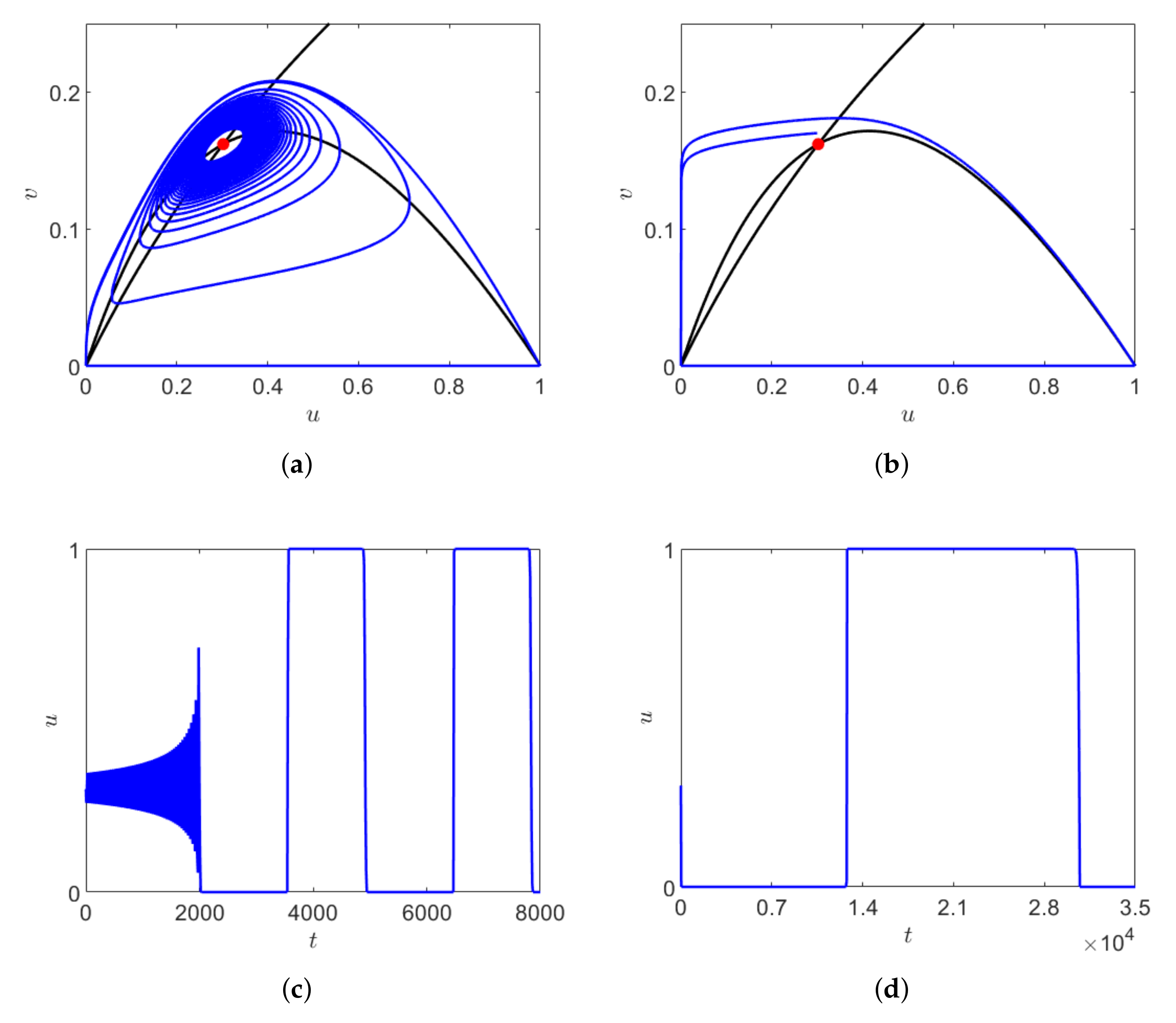
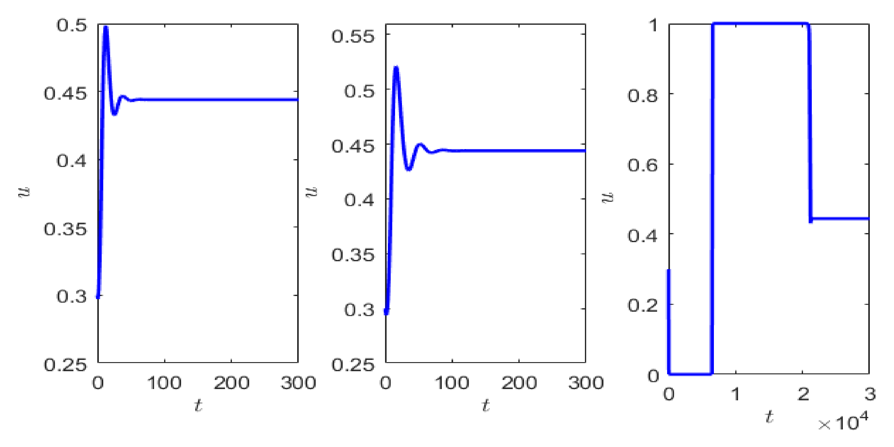
Figure 7. The phase space (upper panel) and the corresponding dependence of the prey density on time (lower panel) showing the transient dynamics for $\beta =1.008502,\delta =0.35.$ (a,c) $\epsilon =0.53,$ (b,d) $\epsilon =0.05.$ Red dot represent the unstable equilibrium point. Other parameters are fixed as above.

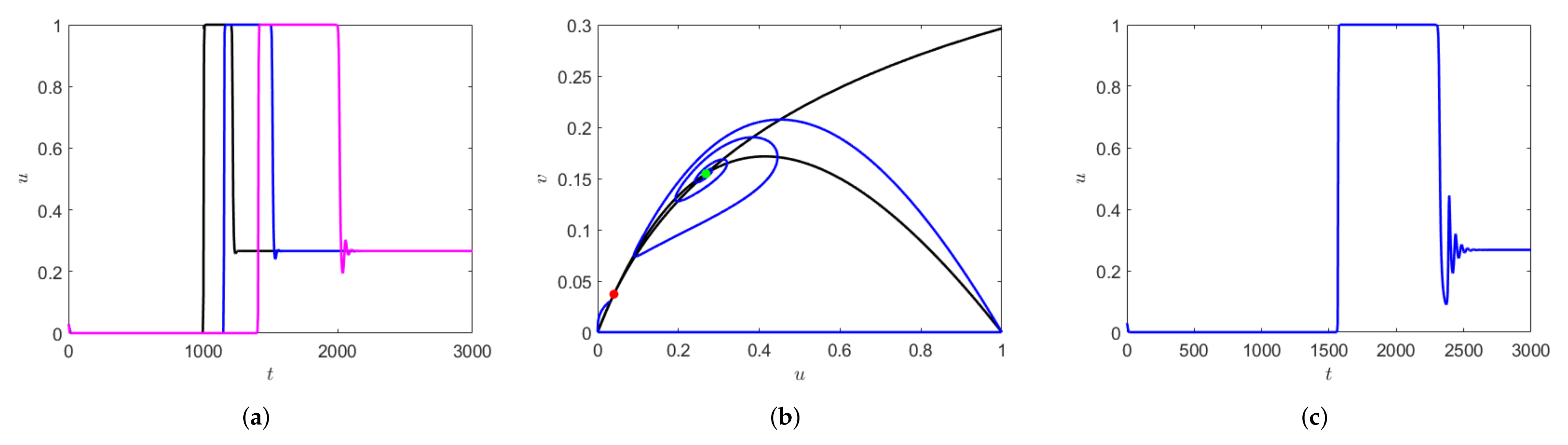
For $\beta =1.24,\delta =1.2$, the system has two coexistence equilibrium points where $E_{1*}$ is the saddle point and $E_{2*}$ is stable focus. Starting from initial point close to $E_{1*}$, with decreasing $\epsilon$ the duration of transient dynamics increases and the system stays near the origin for a longer time. Here, the long transient arises due to the crawl-bys behavior of the saddle point $(0,0)$ and $(1,0)$ and also due to the slow growth of the predators. With decreasing $\epsilon$, the trajectory approaches the saddle point $E_{1*}$ through a trajectory passing through the close proximity of the stable manifold, where the system spends a longer time and the chaotic oscillation increases before converging to $E_{2*}$. This is another example of long transient. The solution of system (1) obtained for three different values of $\epsilon$ is shown in Figure 8a for $\beta =1.24$ and $\delta =1.2.$ The phase space trajectory and the corresponding dependence on time obtained for $\beta =1.239254$ and $\epsilon =0.52$ are shown in Figure 8b,c, respectively.

Figure 8. (a) The prey density as a function of time obtained for $\beta =1.24,\delta =1.2$, and three values of $\epsilon$ (which are marked in the figure legend); (b,c) phase space and corresponding plot of the prey density for $\beta =1.239254,\epsilon =0.52.$ The red and green dot represent the saddle and stable equilibrium point, respectively. Other parameters are fixed as in Figure 1.

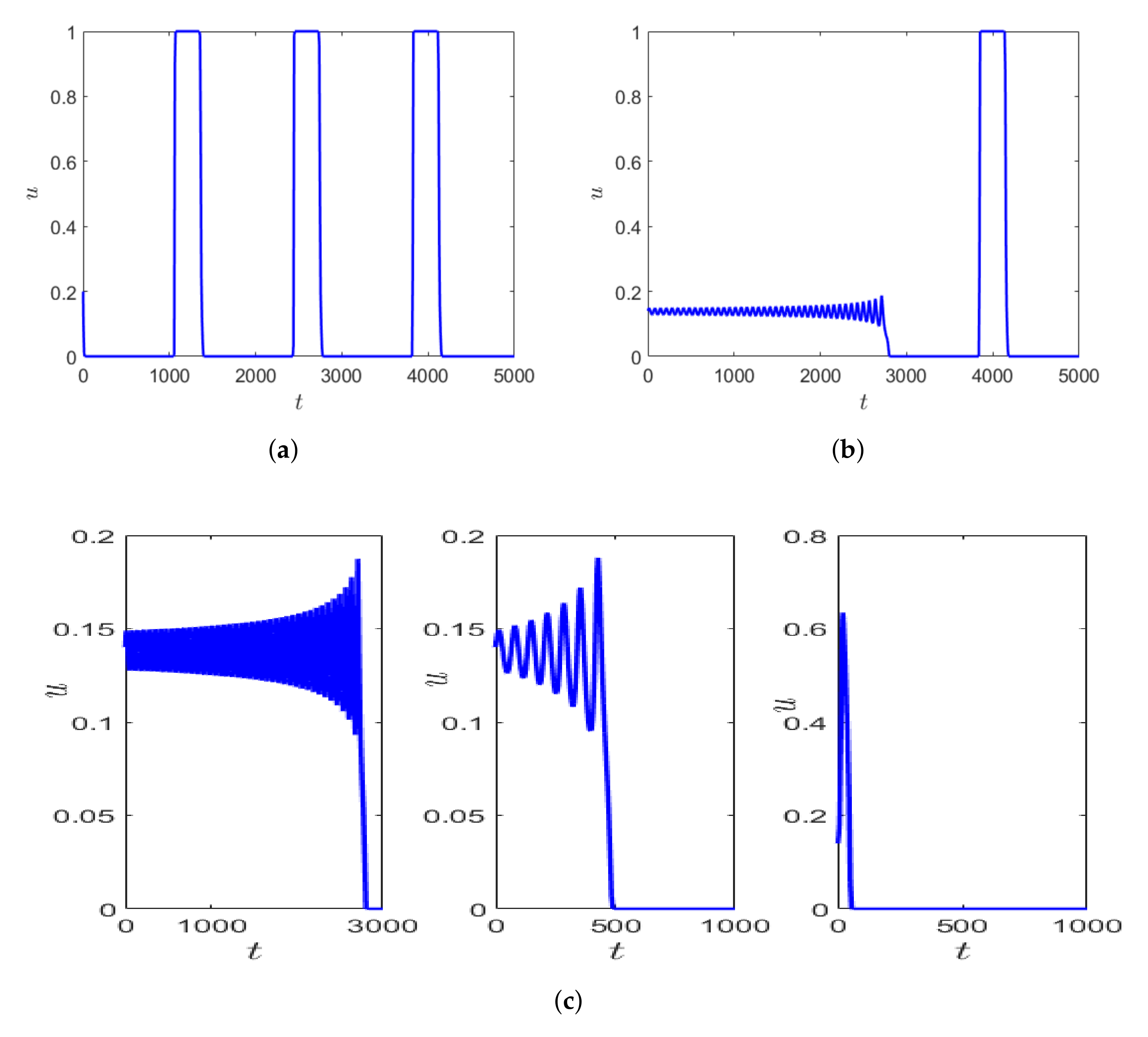
Depending on the initial values of prey and predator density, the system can exhibit longer transients. This is represented in Figure 9a,b, where the parameter values are kept fixed as mentioned in the figure caption, but simulated with varying initial conditions. The number of oscillations exhibited by the prey population differs significantly within the fixed time interval of time, say $t\in [0,5000].$ Additionally, using the same initial condition as in Figure 9b but slightly decreasing $\epsilon$, the oscillatory transient decreases, but the nature of the transient remains the same before converging to the periodic orbit which is relaxation oscillation (Figure 9 (left, middle)). This similarity in the local dynamics of the system can sometimes be seen as an early warning signal for drastic change in population dynamics of the species [21]. Figure 9c shows the zoomed version of the initial transient of the solution trajectory before converging to relaxation oscillation. If we decrease $\epsilon ,$ we observe that the initial oscillations in prey density decreases and the prey density is almost negligible until time about $t=1000$ for $\epsilon =0.1.$ (e.g., see the right-hand side in Figure 9c).

Figure 9. Solution of system (1) showing the prey density as obtained for $\beta =1.21,\delta =0.847,\epsilon =0.9135$ with different initial data (a) $(0.2,0.2)$ and (b) $(0.14,0.104).$ (c) Zoomed version of the initial transients before converging to periodic orbit for $\epsilon =0.9135,$ (left) $\epsilon =0.9$ (middle), and $\epsilon =0.1$ (right), respectively.

6. Discussion

Prey–predator models with a slow–fast time scale are mainly studied for the systems involving prey-dependent functional responses. For classical Gause type prey–predator models with prey-dependent functional response and linear death rate of a specialist predator, the steady-state coexistence loses its stability when the non-trivial predator nullcline passes through the fold point (cf. Section 2 and Section 3). The non-trivial predator nullcline is then a vertical straight line and stable coexistence equilibrium loses stability through supercritical Hopf bifurcation when the functional response is not only prey-dependent but, more generally, monotonic [6,7]. In the presence of slow–fast time scales, in case $ϵ\ll 1$ the stable oscillatory coexistence scenario can change to relaxation oscillation through canard explosion. Interesting dynamical consequences are observed when the functional response also depends on predator density and predator growth is affected by intra-specific competition and also the prey growth is affected by the Allee effect [7,22]. The main intention of our current work is to consider the effect of slow–fast time scale on the dynamics of a prey–predator model with ratio-dependent functional response and Bazykin type growth equation for the specialist predator where the predator mortality includes a quadratic term.

The dynamics of the model under consideration has some remarkably distinguished features when compared to the classical Gause type models. Depending upon the parametric restrictions, we find one or two coexistence equilibrium points. It is true that the destabilization of coexistence equilibrium is through Hopf bifurcation, but the magnitudes of the parameters determine whether it is super-critical or subcritical. Interestingly, we find a large amplitude stable periodic solution which originated through a global bifurcation, and saddle node bifurcation of limit cycle is also possible. The large amplitude periodic solution changes to relaxation oscillation for $\epsilon \ll 1$. This phenomena is responsible for the transition of stable coexistence to relaxation oscillation without the canard explosion. This is a new finding in the context of slow–fast dynamical systems. Further, with the help of numerical simulation, we showed the existence of two different types of canard explosion occurring in the system. When the Hopf bifurcation is supercritical, for $\epsilon \ll 1,$ the transition from small amplitude stable Hopf bifurcating cycle to large amplitude relaxation oscillation takes place via a family of canard cycles which are stable. In contrast, the intermediate canard cycles are unstable whenever the Hopf bifurcation is subcritical.

The effect of multiple time scales is known to be one of the main dynamical mechanisms resulting in the emergence of long transient dynamics [8,12,20]. The long transients are usually associated with the slow phase of the dynamics (cf. Equation (3)) where the system’s dynamical variables (in our case, u and v) closely follow one of the system’s nullclines [2]; in the case of a prey–predator system with a much faster growth rate of prey ($\epsilon \ll 1$), that will be the predator nullcline. Correspondingly, it results in the prey density periodically falling to very small values (as $\left\{\right(u,v\left)\right|u=0,v\ge 0\}$ is a part of the predator nullcline) and remaining at low values for a considerable duration of time before starting growing again (cf. Figure 7 and Figure 9): a long transient dynamic that may give a misleading impression of prey going extinct.

The above may have important ecological implications. Prey density remaining at low values over a considerable time may, in realistic terms (even that in mathematical sense the prey density never becomes exactly zero), be regarded as prey extinction. Note that this happens just as a result of an increase in the time scale ratio, without necessarily changing any other parameters. Thus, rather paradoxically, a sufficiently large increase in the growth rate of prey may lead to prey extinction and the system’s collapse. A more specific ecological interpretation can be given depending on the factor resulting in the prey growth rate increase. In case such an increase occurs as a result of environmental change, the situation is similar to the well known paradox of enrichment: something that is intuitively expected to make a positive effect on the population dynamics would instead result in system destabilization and eventual species extinction. Alternatively, an increase in the prey growth rate may occur as a result of species evolution; in this case, the corresponding change in the system dynamics resulting in the prey extinction can perhaps be termed as an evolutionary suicide.