Abstract
As the amount of historical data available in the legal arena has grown over time, industry specialists are driven to gather, compile, and analyze this data in order to forecast court case rulings. However, predicting and justifying court rulings while using judicial facts is no easy task. Currently, previous research on forecasting court outcomes using small experimental datasets yielded a number of unanticipated predictions utilizing machine learning (ML) models and conventional methodologies for categorical feature encoding. The current work proposes forecasting court judgments using a hybrid neural network model, namely a long short-term memory (LSTM) network with a CNN, in order to effectively forecast court rulings using historic judicial datasets. By prioritizing and choosing features that scored the highest in the provided legal data set, only the most pertinent features were picked. After that, the LSTM+CNN model was utilized to forecast lawsuit verdicts. In contrast to previous related experiments, this composite model’s testing results were promising, showing 92.05 percent accuracy, 93 percent precision, 94 percent recall, and a 93 percent F1-score.
Keywords:
court judgment prediction; judicial data; deep learning; neural networks; feature selection MSC:
6204
1. Introduction
With the introduction of artificial intelligence, data mining applications have become increasingly frequently used in a variety of fields, including commerce, academia, medicine, and litigation. Computational approaches, such as those used in other disciplines, allow the law sector to gather and evaluate a large amount of legal data available in judiciary archives. Furthermore, examining such judiciary data to forecast legal outcomes not only reduces the strain on court employees but also allows for prompt decision-making, resulting in the effective processing of cases [1].
1.1. The Importance of Forecasting Court Case Judgements
The basis of each lawsuit in the field of law is complicated since there are many linkages and interconnections between existing instances, and a jury’s conclusions for comparable cases should be nearly the same. However, the intricacy of a case, as well as the presence of human participation, frequently results in different outcomes for cases that are otherwise comparable. As a result, computational and predictive algorithms can aid courts and attorneys in making the best decisions possible, thereby resolving such issues. Moreover, this may assist non-legal specialists in comprehending the fundamentals of a certain case or situation [2].
Deep learning (DL) is a new branch of computer science that automatically extracts from previous data and efficiently predicts outcomes using a sophisticated set of feature embedding algorithms [3]. It is used to forecast stock prices [4], personality recognition [3], disease prediction [5], text categorization [6], and others [7]. Data scientists in the legal field are encouraged to develop practical solutions that will assist lawyers and judges in accurately forecasting judicial judgments [1,2]. As a result, it is critical to research and apply cutting-edge DL techniques to historical records from the legal arena for the accurate assessment of judicial outcomes.
1.2. Research Motivation
Several works looked at leveraging historic judicial records to forecast judicial decisions exploiting computational methods such as machine learning [1,8]. However, the central emphasis of these investigations, was entirely on the earlier detection of judicial case judgements. They were also constrained by (i) a limited choice of predictors utilized to represent court case judgments and (ii) conventional encoders that attempted to address the connection between the predictors in the judicial dataset. As a result, the LSTM+CNN model developed in this work took advantage of enhanced feature selection strategies. An RFE test was employed in the first phase to determine effective predictors for court case judgments. In the following stage, a long-term, short-term memory (LSTM) and a convolutional neural network (CNN) were employed to anticipate court judgments from a given legal set of data.
1.3. Baseline Work
We employed machine learning to model a system for forecasting judicial case judgments based on past judicial data [1]. It is intended to anticipate court outcomes using machine learning techniques such as support vector machines (SVM), k-nearest neighbors (KNN), and naive Bayes (NB). While choosing effective predictors ahead of applying machine learning to huge data sets may provide remarkable results, machine learning classifiers utilize a traditional encoding method that does not capture the overall connections between predictor variables in a machine learning-based data set [3]. As a result, traditional machine learning classifiers may not provide an effective technique for forecasting judicial cases from judicial knowledge.
To overcome the shortcomings of this baseline study [1], we developed an efficient feature selection approach augmented with a deep learning model (LSTM+CNN), which was previously effectively used in a wide range of applications, including personality classification [3], plant disease classification [6], concept-level sentiment analysis [9,10], and others [2]. We used an RFE test to pick features and, subsequently, an LSTM+CNN model to predict court cases.
The process is as described in the following: (i) an RFE test was used to identify highly ranked features that contribute significantly to forecasting judicial case judgments; (ii) the LSTM model makes use of context by maintaining long-term interrelationships; and (iii) the convolutional neural network (CNN) system forecasted court case judgments effectively. As a result, the suggested technique offers the advantages of both optimum feature selection and LSTM and CNN layers for predicting court case judgments from past judicial records.
1.4. Problem Statement
Prior to actually going on to model design and development, it is required to first describe the prediction problem. Using past judicial data to forecast court case judgments is difficult owing to several reasons, including inadequate predictors choice, sparse judicial data sets, and the usage of conventional feature sets accompanied by ML algorithms [1,8,9]. Additionally, resulting from poor predictors choices and a lack of hybrid models, DL models are less efficient when used in court case prediction. To address these challenges, we consider forecasting judicial case judgments from judicial data to be a multi-criteria prediction problem in which the court judgment is predicted from a given judicial data collection. The problem statement in this research is described as follows: A flow of legal training data ‘CD = [cd1, cd2, cd3,...cdn]’ was fed into the system in order to forecast the ultimate court judgement, i.e., T1 (affirm), T2 (reverse), and T3 (other). Our objective was to develop a deep learning model that learnt from supplied training data in order to predict the final court judgement in the judicial domain using a deep neural network model with enhanced feature selection.
1.5. Research Objectives
Table 1 show the study objectives that were addressed in order to efficiently forecast court case judgments.

Table 1.
Research objectives.
1.6. Research Contributions
This paper makes the following research contributions:
- The use of recursive feature elimination (RFE) to rank and choose optimal features is critical for forecasting court judgments.
- The use of a deep learning model (LSTM+CNN) to forecast court judgments.
- Evaluating the effectiveness of traditional machine learning classifiers vs. the proposed deep learning model in predicting court judgments.
- Prediction of court judgments in terms of three decision classes.
- Evaluating the suggested approach’s effectiveness against other deep learning and benchmark research.
- The suggested approach increases the performance of the model for court case judgments by a substantial margin.
The remainder of this study is arranged as follows: Section 2 outlines the existing literature, whereas Section 3 explains the suggested approach’s methods. The findings and discussion are presented in Section 4, and the conclusion and future applications for the suggested technique are presented in the final section.
2. Review of Existing Literature
This section provides an overview of prior legal research on lawsuit forecasting.
Several machine learning (ML) classifiers were already used recently to forecast judicial case judgments based on past judicial records. Using a machine learning classifier and a large legal database, [1] researched and used more effective collections of predictors. Experiments showned that including feature selection into predictive classifiers improves their performance substantially. [11] used a random forest (RF) classifier to analyze data from the United States Supreme Court. The selection of effective indicators prior to implementing machine learning on a big data set may have provided more promising outcomes, despite the fact that their system attained good accuracy in the cases and voting level judgments. Following the extraction of features, [12] suggested an SVM classifier for the prediction of court verdicts in criminal cases. Despite the fact that their method was more than 80% accurate, more research is needed because it only dealt with a small portion of the criminal proceeding data. A supervised machine learning approach, SVM, was developed by [13] to forecast decisions made by the French Supreme Court. The method was combined with a traditional feature extraction scheme, which was centered on an n-gram structure. In addition, n-fold cross-validation was performed to examine the outcome of the research. Their model, on the other hand, must be improved in order to evaluate the balanced data. Word embedding and other sophisticated feature engineering approaches are employed in deep learning (DL) models to improve the performance of ML techniques. [14] suggest a neural network that uses attention to recognize the charge and retrieve all potential articles in each situation. When constructing the suggested model, a variety of methods were employed, including support vector machine learning (SVM), a neural network model (Bi-GRU), and stochastic gradient descent with positional labelling (SGDLP). Cases involving many defendants could not be effectively handled with this approach, so it must be enhanced in this regard. Using the legal factual summary of the case, an official report and a judicial declaration may be generated automatically. On the other hand, [15] developed an LSTM-based encoder and decoder system. The collection consists of court records from China. However, the approach was restricted in breadth since it only prioritized situations with one charge and one defendant, excluding cases with several allegations and defendants. However, by incorporating more advanced approaches such as reinforcement learning, the system’s efficiency might be increased. To identify the result of criminal trials based on official case factors, [16] used a deep learning model that used neural networks to predict the outcome. This was conducted by utilizing an attention mechanism and Bi-GRU with DL. The Thai Supreme Court provided the data set of 1000 criminal proceeding verdicts. There were good findings from the model, with a 66.67% accuracy. However, the study’s shortcomings include the fact that it only looked at criminal instances, and the model’s effectiveness can only be improved by incorporating more attention processes. Prediction models were also developed using hybrid DL models. [2] used DL and ML models to make predictions about violations of human rights. They used Bi-GRU to analyze data from the public database of human rights. In spite of the model’s higher performance in terms of enhanced accuracy, f-measure, precision, and recall, hybridized deep learning models with optimum sets of attributes may still be built upon to even further enhance it. Numerous other methods were employed in addition to machine learning and deep learning models in order to forecast court judgments. On various data sets taken from Chinese court papers and encoded using the cascaded jump approach, [17] discovered that topology training is an innovative technique for predicting multitasking judgement learning and, therefore, for rendering judgement prediction. In spite of the fact that it had several shortcomings, including a lack of familiarity with numerous charges, the system could deliver effective outcomes if such shortcomings were properly resolved. [18] suggested a key phrase information gathering approach for court documentation. Semantic-driven searches were performed on the data collection of articles, including Indian Supreme Court rulings, using approaches such as POS tagging and NER. The inclusion of unnecessary connections in the graph-based approach affected efficiency, even if they were readily deleted. [19] employed Markov logic to recognize breakup decisions and case benchmark datasets from China’s online judgement database. The approach enhanced outcomes for permitted and denied divorce petitions, but the research had a small sample size. Using alternative ML/DL methods could have enhanced the prediction.
The European Court of Human Rights serves as an example of how natural language processing methods may be used to analyze court proceedings and forecast future judicial rulings [20]. The proposed technique predicts violations of nine articles of the European Convention on Human Rights with an overall accuracy of 75%, demonstrating the judicial domain’s promise for machine learning techniques. On the other hand, the authors show, on the basis of previous examples, that making predictions about what decisions will be taken in the future based on previous examples degrades performance (the average accuracy ranges from 58 to 68%).
Hsieh et al. [21] presented machine learning algorithms by providing the randomization feature with an important rating of legal considerations. The experiments show that “the psychological distress losses claimed by the claimant” and “the age of the subject” are important factors in determining how much emotional distress loss there were in fatal traffic collisions in Taiwan.
Gaps in the Research: Although ML employs a traditional machine bag-of-words method as a feature representation technique, this drawback was already effectively solved using cutting-edge word embedding-based approaches in deep learning. However, the problem of managing contextual information through extensive feature extraction and convolutional neural networks should be addressed in order to achieve highly effective prediction of court case judgments employing hybrid deep learning approaches with selecting features and grading.
3. Proposed Methodology
A multi-criteria decision-making solution using deep learning technology is needed to address such a complex prediction problem. Judiciary experts and lawyers may use data, knowledge, and predictions from our framework (see Figure 1) to make judgments about court cases and reduce the burden on legal decision makers. The proposed system structure includes different subsystems, such as (i) data collection, (ii) preprocessing and feature selection, and (iii) predicting court judgments using the LSTM+CNN model.
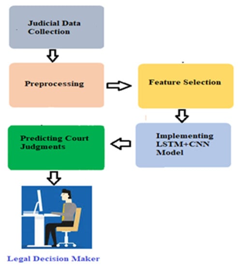
Figure 1.
Proposed system for predicting court judgments.
3.1. Judicial Dataset Collection
We analyzed a sample of US Supreme Court rulings from the judicial repository [22]. This dataset was already frequently utilized by academics to build solutions for court case forecasting since it is not only codified by specialists but also includes detailed instructions on how to encode in the judiciary handbook. The judicial dataset we obtained had 120,506 cases. The judicial dataset contained 27 categorical predictor parameters (Table 2). Professionals expertly encoded these model parameters with different numeric representations, and the explanation of each categorized predictor and its binary values is accessible online at the Court’s webpage [23]. A sample of court cases (without numeric encoding) is shown in Table 2. This manuscript includes a comprehensive data set as supplemental material.
Table 2.
A list of features without feature selection that can be used to make predictions about the judgement of a court case.
To perform the tests, we saved the dataset as a Microsoft Excel sheet, which was then converted into CSV format. The command line parameter “pd.read csv” was used to read the “csv” data source file, which is an important Pandas utility. Using the sklearn train test split function, the original data was divided into two parts: the train set and the testing sets [24]. It was then further divided into 80% training sets and 20% testing sets.
Train set: The model was trained using the training set, with approximately 80% of the data used for the training phase [1]. The training set contained both the output labels (the dependent variable) and the input parameters (the predictor variable).
Validation set: In the proposed methodology, the validation data were also employed to mitigate performance defects such as overfitting and underfitting. As a consequence, a 10-percent validation sample was used for model evaluation or parameterization [3]. In Keras, settings could be adjusted in two ways: manually or automatically. We utilized the automatic verification technique in this research since it provides a fair evaluation of the proposed system.
Test set: The testing data was used to evaluate the effectiveness of the algorithm against previously encountered or unidentified instances. The testing set computed the model’s final estimate [25]. We employed 10% of the test dataset that was independent of the training dataset. Once the system was completely trained, the training data set was only used once. Lastly, the model was analyzed using test data.
Treatment: To validate the model, we employed 10-fold cross-validation. At each training step, 10 training instances were collected. After training on each of the nine subsets of nine folds, the model was assessed on the last “holdout” sample. We selected the model with the greatest F1 score on the holdout sample. Using the final model developed at each training step, one may estimate how well the whole Supreme Court will rule on a certain case. This decision depends on the court’s previous decisions, the tribunal’s previous decisions, and all prior judgments. This practice is comparable to that utilized of a judicial authority when making detailed ex post facto judgments [8].
3.2. Preprocessing
An efficient prediction model needs proper pretreatment of the gathered judicial set of data since a noisy data set causes poor performance of the suggested system. The data preprocessing module includes Handling imbalanced Dataset, optimum feature selection as well as value replacement for null values.
3.2.1. Handling Imbalanced Dataset
The source dataset was substantially unbalanced [1] and was treated unequally across all three categories: T1 = 11120, T2 = 9951, and T3 = 4556. Whenever a model learnt of distorted and uneven classified data, the outcome typically tended to benefit the major class, while the smaller classes were ignored in the prediction phase. This was regarded as a problem of imbalanced classes [24].
To overcome this problem, we created a balanced dataset by employing a data processing sample technique, particularly oversampling, to rebalance all class instances. Oversampling is a technique used to increase the number of minor classes. The most basic technique of oversampling is randomized oversampling, which simply replicates small cases to raise the imbalance proportion [26]. In terms of efficient judicial case prediction, this replica of small class supplementation greatly improved the classifier performance. Algorithm 1 shows a random oversampling Pseudocode.
| Algorithm 1. Pseudocode of random oversampling. |
4. Create synthesis instances at random anywhere along the lines connecting the minority instance and its m chosen peers (where m is a function of the intended level of oversampling). |
Following the use of random oversampling, the balanced dataset was handled similarly across all three classes: T1:1040, T2:1040, and T3:1040. Total instances: 120,506.
3.2.2. Selection of the Most Effective Features
The data set used to forecast court case judgments included a set of possible attributes that might help predict court case judgments. However, before using the prediction system to anticipate court case judgments, an appropriate collection of attributes (predictor variables) had to be chosen [1].
There were a number of potential features in the data set that could be used to forecast court judgments. However, before implementing the prediction system, an ideal collection of features (predictors) had to be determined in order to accurately predict lawsuit outcomes [1]. To select the most optimal attributes from a primary set of data, various approaches such as principal component analysis (PCA) [27], the chi-square (x2) test [12], and RFE [28] could be used.
Yan and Zhang [29] used an RFE to prioritize and choose features from gas sensor data and achieved good results. RFE picks features by evaluating shorter and shorter groups of features iteratively. Firstly, the predictor is learned on the original feature set, and the significance of every feature is determined using any specified variable or iterator. The less significant features are therefore removed from the present list of features. This technique is continued iteratively on the trimmed subset until the appropriate set of attributes is obtained. It is calculated using Algorithm 2.
| Algorithm 2. Optimal feature selection using recursive feature elimination. |
1. 1.1 1.2 2. 2.1 2.2 end 3. 3.1 3.2 end 4. B. Train and evaluate |
On account of the strong correlation with target parameters, the top ten most important features are shown in Table 3. According to their rankings, the top-ranked features are grouped in order of significance to the target class.
Table 3.
A list of optimal features for court judgments.
3.2.3. Null Entries
It is recommended that null entries or missing values be given for data cleaning to solve data discrepancies and optimize the predictive performance of the model [1]. There are three main methods for replacing a missing value: (i) directly compute the average and place this in the blank location; (ii) pick one item at random and replace it with the missing value; and (iii) replace the null value with the number of one step prior. We chose the third choice; therefore, the data was filtered by directly replacing the missing value with the proper higher value. Missing values were most typically caused by dividing by 0 when calculating predictors and decision variables on an individual basis [1]. Furthermore, before model training, we preprocessed the dataset and replaced any personal details (e.g., individual identities, ID numbers, addresses, and sexuality) with hyphens.
3.3. A Brief Overview of the Proposed LSTM+CNN Model
The prediction algorithms allows decision-makers to navigate through a number of possibilities and choose the best one. The key elements required to project court case judgments are prioritized as per their RFE relevance score. The suggested LSTM+CNN (long short-term memory + convolutional neural network) model (see Figure 2) for predicting court verdicts operates as follows: (i) feature representation; (ii) the LSTM layer is integrated to maintain long-term interdependence; (iii) a dropout layer is used to reduce the possibility of overfitting; (iv) CNN is used to extract features; (v) a pooling layer is added to reduce the dimensionality of the convolved feature space; (vi) a flattening layer is added to flatten the pooled feature map into a feature set; and (vii) the softmax function is used in the output layer to forecast court case judgments.
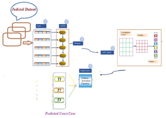
Figure 2.
Overview of the hybrid CNN+BILSTM model for court judgment system.
LSTM layer: In the beginning, an LSTM layer was deployed, which served as an encoder for the data. The input text comprised tokens, and each token was an output token that provided information regarding all previous tokens [3].
Dropout layer: In order to solve the problem of overfitting, the dropout layer employed a parameter called ”rate,” which has a range of 0 to 1 values [3].
CNN layer: As part of the CNN architecture, the convolutional layer obtained improved information content from the LSTM layer and afterwards derived local patterns from that input via a convolutional operation. To construct the convolved feature space, the convolutional procedure employed a content matrix and a filtering matrix. Following that, a rectified linear unit activation function was employed to conduct nonlinear operations [3].
Pooling layer: The pooling layer made use of the maxpooling technique to compress the convolution feature map.
Flatten layer: In the following stage, the flattening layer unrolled all of the entries from the pooled feature map into a feature space, allowing for further treatment.
Prediction of judicial cases at output layer: Finally, inside the output layer, the softmax activation function was used to forecast court case judgments [30]. The softmax function calculated the probability values of the various court judgement classes, with the highest probability class being allocated to the particular lawsuit.
3.4. Detailed View of Proposed Model
The suggested deep learning approach, known as LSTM+CNN, was used to forecast legal case judgments such as T1 (affrim), T2 (reverse), and T3 (other). The suggested LSTM+CNN model has several layers, including an embedding layer, a long short-term memory layer, a dropout layer, a convolutional layer, a maxpooling layer, a flattening layer, and an output layer. The suggested LSTM+CNN model for predicting judicial case judgments from judicial material is depicted in detail in Figure 3.
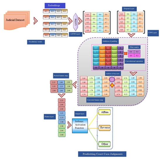
Figure 3.
The suggested LSTM+CNN model’s detailed structure.
3.4.1. Embedding Layer
The process of converting a discrete parameter (class) into a continuous array of numeric values is known as embedding (vectors). Bits in neural networks are low-dimensional matrix encodings of parameters used to train the model. It is desirable to use neural embeddings to minimize the number of features in categorical attributes and to significantly characterize classes in the resulting region. Keras streamlines the embedding implementation process. The obtained judicial data set had input data ‘CD = [cd1, cd2, cd3,...], where the individual data item cd1 was converted into an embedding vector comprising continuous values, where d represents the data embedding dimensionality. The embedding layer was used to create a two-dimensional embedding matrix (feature matrix): MÎ k’ l, where ‘k’ signifies the input data’s length and ‘l’ denotes the dimension of a data embedding. After tokenizing the law data, it was fed to the embedding layer of the deep learning model for treatment, where it was transformed into a matrix of indexes. The embedding layer converted each index in the legal sequence into a vector containing streaming values.
3.4.2. LSTM Layer
The second layer of our suggested approach is the LSTM layer. The embedding matrix is supplied in the long-term, short-term memory layer. This layer performs various computations with the use of four LSTM gates: the forget gate, input gate, candidate gate, and finally, the output gate. Long-term dependencies can be learned by the LSTM layer. Figure 4 depict a pictorial representation of the four gates computations. The computations begin with the forget gate , followed by the input gate , the candidate gate , and the final output gate . The embedding layer’s data is transferred via a long-term memory cell, where computations begin with a forget gate in which the input and the preceding output are multiplied by their weights ,,, and and ,, and . Following that, addition is performed using bias vectors , and . The sigmoid activation function is then used to modify the values between 0 and 1, and values larger than 0.5 are presumed to be 1 for three gates, as shown in the computation below. We used the tangent function for the candidate gate. The final output computation is transferred to the dropout layer.
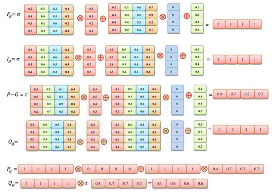
Figure 4.
Calculations of various gate configurations.
Cell state size is indicated by n, and input size is indicated by m. As you can see, shows the vector size of the input gate weight matrices. The mapping weights of ,, and represent the matrices of the output gate. , and are the bias vectors. τ stands for the hyperbolic tangent function, and σ stands for the sigmoid activation function. Below is a list of all the gates’ calculations.
3.4.3. Dropout Layer
The primary goal of this layer is to avoid overfitting. The 0.5 value represents the “rate” parameter, which has a value between 0 and 1. The dropout layer casually deletes or randomly switches off neuron activity in the LSTM layer, depending on the application of dropout on the LSTM layer. Dropout modelling on a single neuron is shown in Equation (7).
r represents the intended outcomes, whereas s is the probability associated with real-valued word representation. As a result, if s = 1, the neuron with a real value is eliminated; otherwise, it is activated. Figure 5 depict the operation of a dropout layer. The embedding layer contains a real-valued depiction of certain data. As demonstrated in Figure 5, when the dropout layer is applied, certain values inside an LSTM layer deactivate at random.
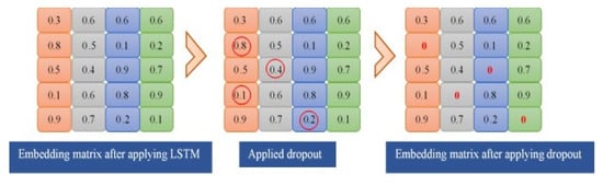
Figure 5.
Using a dropout layer.
3.4.4. Convolutional Layer
During the execution of this layer, a convolutional operation takes place, which is a mathematical operation executed over two functions, leading to the formation of a 3rd function. This procedure can be carried out by rearranging the dimensions of the (n) input matrix, the (t) filter matrix, and the (o) outcome matrix in the following ways:
In Equation (8), N is the input matrix, which is formed by the LSTM layer, denotes all real values, u denotes the length, and v denotes the width of the input .
As shown in Equation (9), T stands for the filter matrices, stands for all real numbers, g stands for length, and .stands for the filter matrices’ breadth.
where in Equation (10), O is the output matrix, denotes all real numbers, w denotes length, and x denotes the output matrix’s width, which is denoted by .
Equation (11) show how to produce a convolutional operation.
The elements of the output matrix O are represented by the letters , the elements of the filter matrix T, are represented by the letters , element-wise cross multiplication is represented by the letter (⊗), and the element related to the input matrix N = is represented by the .
For example, the following convolutional operation is conducted on the dataset’s initial data stream: (i) the components of the input matrix are 0.3, 0.6, 0, 0.5, (ii) The elements of the filter matrix are 0.8, 0.5, 0.4, 0.2, and (iii) the convolutional operation is 0.3 0.8 + 0.6 0.5 + 0 0.4 + 0.5 0.2 = 0.64, where 0.64 is the first element of the convolved feature map. Similarly, the element-wise cross multiplication and addition procedures continue until all of the values in the input matrix are covered, which will be accomplished by sliding a filter across the input matrix.
Feature Map
Once bias and activation functions are added to the convolved map, a feature map for a desired sentence is computed as described in Equation (12).
After adding the bias and activation component to the convolved mapping, a feature map for specified data is produced as defined in Equation (12).
A feature map has the dimensions = = where b is the bias term and f is the activation function. In the rectified convolved feature map, the items are shown in the order they are presented:
Following the convolutional process, the elements of every output matrix are simply added to the bias term.
For example, adding a bias factor to the first member of the output matrix yields 0.64 + 1 = 1.64, which represents the first item of the feature map for a particular text (see Figure 6).
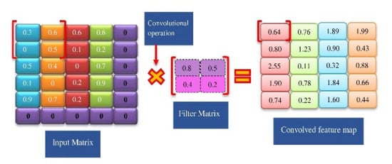
Figure 6.
Convolution of the input and filter matrices.
The parameters used in this layer, as shown in Algorithm No. 1, are: (i) “filters,” which displays the number of filters in the convolutional layer; (ii) “kernel size,” which displays the dimensions of the convolutional window; and (iii) “padding,” which retains a specific value among the three values, namely “valid,” “same,” and “casual.” If padding has the value “valid,” it means there is no padding. The term “same” padding indicates that the original data length is identical to the output length. Furthermore, if padding has the value “casual,” it will generate expanded convolution; (iv) the parameter “activation = Relu” demonstrates that activation is used to reveal nonlinear behavior.
Ultimately, a feature map is created and the Relu activation function is employed to remove non-linearity. Its mathematical description is as follows: output = max (zero, input), where input is a feature map item. In the input data, for example, the first item in the feature space is 1.64. When the Relu activation process is conducted towards it, output = max (0, 1.64) changes to output = 1.64, since 1.64 > 0. As a result, other corrected feature map pieces are computed for the particular data stream (see Figure 7).
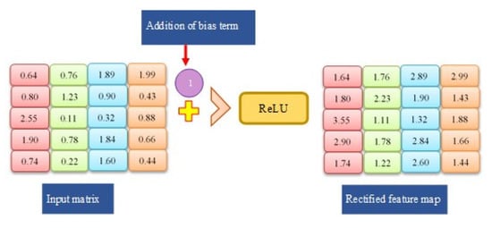
Figure 7.
Applying Relu Function and addition of bias term.
3.4.5. Pooling Layer
The dimensionality of the feature map is reduced by obtaining information using the pooling layer. As a result, every sentence data input into a dataset is subjected to max pooling. By employing max pooling, the needed feature of a data stream is achieved by picking the largest value. Equation (13) show the formula for the pooling layer.
represents the items of the pooled feature map.
The pooled feature map’s length and width are indicated by P ϵ . In this case, s stands for length, and t represents width. The “MAX” function is used to pick the top weight.
A pooled feature map is generated in such a manner that the window size is set to (2 × 2), the feature map is put on it, and lastly, the maximum element is retrieved from inside the window. In this instance, the highest item is 2.23, which also reflects the first item in the pooled feature map connected to the given data input among the window sizes chosen, i.e., max (1.64, 1.76, 1.80, and 2.23). As a result, a similar method will be followed for the supplemental values in the pooled feature map (see Figure 8).
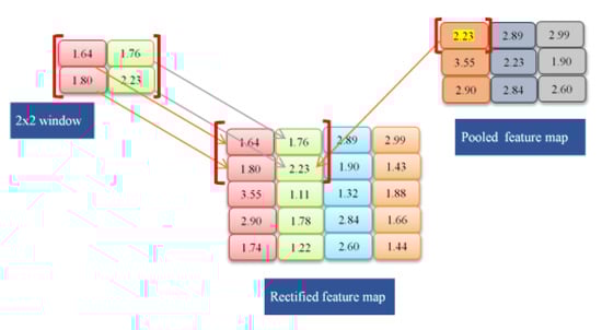
Figure 8.
Applying maxpool operation.
3.4.6. Flatten Layer
This layer of the convolutional neural network converts the pooled feature map to a single vector, which is then fed into the neural network for prediction. For the required sentence, the feature map is represented as a single vector. To accomplish the flattening of the pooled feature map, as described in Equation (14), the reshaping operation of NumPy is used, which results in rows of feature vectors that are concatenated.
Flattening = pooled. reshape (4 × 2, 1)
The provided equation contains rows 1, 2, 3, and so on, and then attaches them all to create a single column vector. The flattened layer’s objective is defined in Figure 9, in which the matrix indicates the pooled feature map for specific data input and a single column vector representing the flattening operation that is conducted on a data stream pooled feature map.
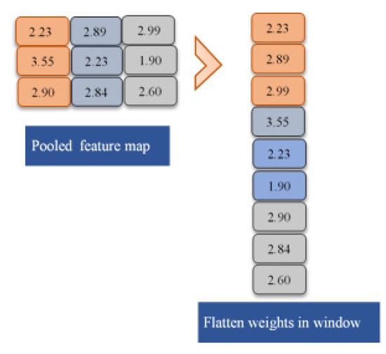
Figure 9.
Flatten layer.
3.4.7. Output Layer
The CNN layer’s final output is utilized as input to the output (final) layer, which uses the softmax algorithm to forecast court judgments. The following equation is utilized to generate the final output (see Figure 10).
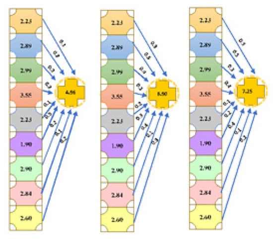
Figure 10.
Output of calculation.
Equation (15) has n as the input, k as the weight, and q as the bias value.
The “softmax function” is employed in order to compute the probability (see Figure 11).
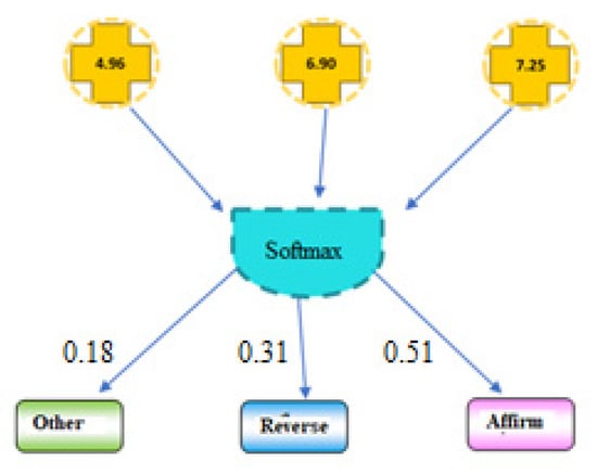
Figure 11.
Classification of court judgments.
The T1 court case judgement had the highest probability. In this trial, the forecasted court judgement is “affirm” (Figure 11). The pseudo-code steps of the suggested system are depicted in Algorithm 3.
| Algorithm 3: Pseudocode of proposed Court Case Judgments Prediction model. |
Model=Sequential() # using Embedding Layer to map integers to low dimensional vectors Model.add (Embedding()) #—Applying LSTM layer for context information extraction Model.add (LSTM(100, return_sequence= true))) Dropout Layer for preventing overfitting Model.add(Dropout(0.5)) #Prediction of court case judgement using Softmax function Model.add (Dense(3, activation=‘softmax’)). # Compilation Function model. compile (loss = binary_crossentropy, optimizer = adamax, metrics= [accuracy]) #Evaluate model on test data court_case_judgement= model. evaluate () # Returning predicted court case judgement: “T1”, “T2”, “T3” Output: return judgement End Procedure |
3.4.8. User Interface
This section presents a software interface for forecasting court judgments written in Python and deployed with the Keras library [31]. Court judgement forecasting software is designed to help justices and lawyers make the correct decision. For simplicity and consistency, it was divided into modules based on the recommended approach. Three key modules make up the application’s structure: (i) a module for collecting data and preprocessing it; (ii) learning a classifier and model; and (iii) court judgement forecasting.
(i) Data gathering and preprocessing component: This module needs court case data input. After that, the data is preprocessed in the backend. The database is updated with much better data, and for each lawsuit, a unique case identifier is created. As a result of preprocessing, classifier implementation is carried out, and a model is developed that could be used to predict the result of court cases. The court case forecasting module makes predictions about the findings of a court’s ruling depending on the actual data that has been entered. After entering the relevant data into the system, a distinctive lawsuit identifier is obtained, which is used to identify and track down each individual case. The interface shown in Figure 12 is used to input and preprocess data for a new input of the case. As previously stated, data is preprocessed at the backend of the application. The template that we developed is dynamic in nature, and the attributes of the form may be tailored to the requirements of each lawsuit.
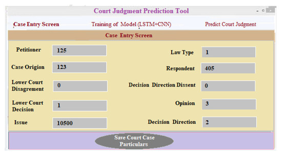
Figure 12.
Application for entering data for court judgment prediction.
(ii) Training of the building model (LSTM+CNN): Figure 13 show a training set to display a dataset of judicial predictor variables that can be used to train classifiers and build models. This screen appears when a user selects the “Model Train” tab and the data loaded for training is presented. After clicking “Model Train”, a trained model is created.
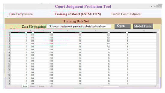
Figure 13.
Create an interface that loads the training data.
(iii) Predicting court judgment: Predicting the outcome of a court case is as simple as entering the relevant case information and clicking the “Predict Court Judgment” button. An updated training set is created when the “update training set” button is selected. When the user enters the case information and clicks on the “predict court decision judgment” tab, the outcomes are shown as “T1: affirm”, “T2: reverse”, and “T3: other”, along with a forecasted degree of confidence for each choice made. For a particular set of criteria, “T1: Affirm” is the expected outcome in a court case, as shown in Figure 14.
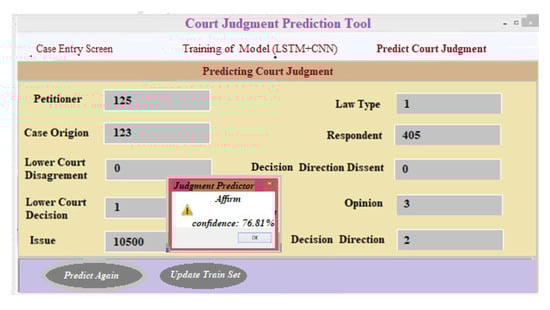
Figure 14.
Interface for predicting the outcome of a court case.
4. Results and Discussion
This section describes the scientific results gained from a set of experiments undertaken in order to address the research questions provided in Section 1.
4.1. Addressing Research Objectives
4.1.1. RO1: To Forecast Court Case Judgments Using LSTM+CNN on the Basis of Historical Judicial Data
To accomplish the aforementioned research objective #1, we used different LSTM+CNN models to forecast court judgments using historical judicial data by modifying the parameters of the proposed LSTM+CNN model. The following settings were used: vocabulary vector size (53), embedding dimension (128), softmax activation function, dropout value (0.5, 0.8, 0.9), LSTM unit size (10, 15, 20, 30, 50, 60, 80, 100, 130, 150), number of epochs (7), number of filters (10, 16), filter size (8, 10), number of convolution layers (1), number of hidden layers (3), and batch size (8, 16, 32).
The following equations (Equations (17) and (18)) were used to calculate precision and recall.
As follows, Table 4 show the results of each class’s precision computations using Equation (17). For each category, we obtained P1, P2, and P3, the precision, Tc1, Tc2, and Tc3, and the true positives for each class, respectively.
Table 4.
LSTM-CNN deep learning models’ precision.
Table 5 show the results of calculating the recall for each class using Equation (18). Tc1, Tc2, and Tc3 are the actual/true classes, and R1, R2, and R3 are the corresponding recalls; meanwhile, Tc1, Tc2, and Tc3 are the corresponding true positives.
Table 5.
LSTM-CNN deep learning models’ recall.
Specifically, Equations (19)–(24) were used to compute the macro- and micro-averages of precision, recall, and F-measure, and the results are provided in Table 6.
Table 6.
Performance measures of LSTM+CNN court case prediction models.
According to the data shown in Table 6, the best performance was achieved using LSTM+CNN-model 10, which outperformed all other LSTM+CNN models.
Table 7 show the accuracy, precision, recall, and f-score of the LSTM+CNN model (with and without feature selection).
Table 7.
Evaluation of the LSTM+CNN model’s performance with and without feature selection with feature selection.
Table 8 display the training duration, test accuracy, and test loss for all 10 trials with varied parameter values in the LSTM+CNN model. The LSTM+CNN-10 model, with filter sizes (8), filters (16), and LSTM unit size (10), achieved the greatest accuracy (92.05%) of all the examined models.
Table 8.
The LSTM+CNN models’ test accuracy, test loss, and training time.
Table 9 show that when compared to not using feature selection, including features in the model significantly reduces the number of calculations required in terms of training and testing time while also improving accuracy. The experimental data and complexity analysis demonstrate that the proposed model may be used to anticipate court outcomes in actual environments with a high degree of accuracy in court forecasting scenarios.
Table 9.
Comparison performance with feature selection and without feature selection (training vs. testing times).
4.1.2. Runtime Overhead of the Suggested LSTM+CNN with the Traditional SVM
Computation costs are shown in Table 10 as a sum over the entire number of multipliers applied to a single frame of data in convolution-based layers for the forward run. It is also possible to compute the total number of learnable model parameters. Using the LSTM+CNN, Table 10 contrast the efficiency of the suggested approach with that of a standard SVM, and the results are encouraging. It also demonstrates that using LSTM+CNN improves accuracy by 0.7 percent while reducing computational costs when compared to regular SVM. Experiments and complexity analyses show that the model can be used to predict court cases with a fair amount of accuracy.
Table 10.
Performance of LSTM+CNN (proposed) and classical SVM.
4.1.3. Complexity of the Proposed Algorithm
Complexity of LSTM: Ultimately, we need to determine the time complexity of the LSTM+CNN algorithm. To accomplish this, we first need to compute the LSTM layer’s and the convolutional layer’s time complexity. Because LSTM is spatially and temporally local [23], the input length has no effect on the network’s storage needs, and the time complexity per weight is O(1) for each time step. In other words, the total amount of time it takes to build an LSTM is O (w), where w is the number of weights.
Complexity of CNN: According to [21], the complexity of all convolutional layers can be approximated by the equation , where k is the number of convolutional layers, is the number of filters in the jth layer, x is the number of input channels in the jth layer, Pj is the spatial size of the filter, and Yj is the spatial size of the output feature map; all of which are constants.
Complexity of LSTM+CNN: The complexity of the LSTM+CNN per clock cycle may be estimated as the summation of the complexity of the LSTM layer and the complexity of the convolutional layers: w). It is because of this that we can infer that our model has O complexity when it is written in the standard asymptotic nomenclature.
4.1.4. Effect of Parameters on Computation
We conducted different experiments to measure the effects of parameters on the model’s performance. Model hyperparameters include batch size α, number of convolution kernels (β), size of convolution kernel (γ), and optimizer (ε). There are some hyperparameters that can only be set manually and cannot be changed automatically during training. This has a big impact on the model’s performance.
Batch size(α): α is the number of training samples the neural network has, which tells us how many samples we will use to figure out how much we lost in each optimization step.
Number of convolution kernels (β): β is the number of convolution kernels utilized in convolution, and how many feature maps will be created after convolution.
Size of convolution kernels (γ): The size of convolution kernels is represented by the symbol γ. Convolution kernels have length, breadth, and depth. Convolution kernel length and breadth must be manually set in a CNN convolution layer.
Optimizer ε: When optimizing loss and then updating weight parameters, the kind of optimizer employed is known as Optimizer ε.
Therefore, we looked into how these “super parameters” might affect the performance of our hybrid LSTM+CNN model. We propose a hybrid LSTM+CNN model with the following parameters: a = 512, β = 4, γ = 13, and ε = Adam. The following are the model training outcomes for some of these specific parameters.
Role of Batch_size α: Figure 15 show the results of our trials with “α” set to 128, 256, and 512. When a=128, the training loss converges quicker and reaches the set iterations in the same duration. Although a smaller batch size might speed up the optimization, this means that more computation time is required to optimize. The running speed and gradient decline direction can be improved by suitably increasing the batch size. The amplitude of training vibration is reduced in proportion to increased accuracy.
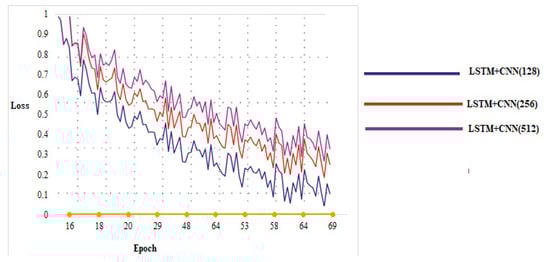
Figure 15.
Study of the parameter (α) of training loss.
Role of Number of convolution kernels (β): Figure 16 show the results of our experiments with different numbers of “β” (1, 2 and 4) convolution kernels. We obtained 0.9403 accuracy with one convolution kernel. The loss convergence rate grows as the number of convolution kernels doubles. With a value of four, the rate of loss convergence is considerably increased. In general, the deeper the network is, the more convolution kernels are needed to obtain all of the important characteristics.
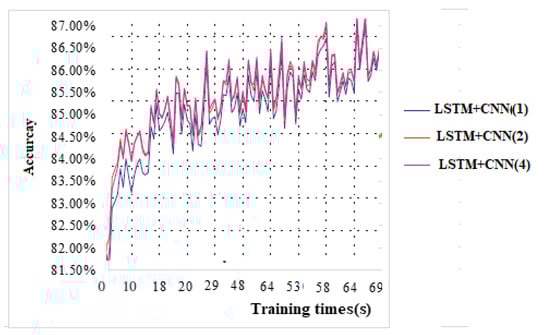
Figure 16.
Study of the parameter (β) of training accuracy.
Role of Size of convolution kernels (γ): In trials with convolution kernels of sizes 1 × 2, 1 × 3, and 1 × 4, as indicated in the graph (Figure 17), it is noticeable that when the convolution kernel is 1 × 2 in size, the validation loss will fluctuate drastically. For a 1 × 3 or 1 × 4 convolution kernel, loss converge is faster, and the fluctuation range is less hence it is better to use a larger convolution kernel.
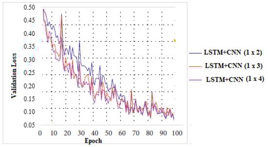
Figure 17.
Study of the parameter (γ) of validation loss.
4.1.5. RO2: To Compare the Efficiency of the Suggested LSTM+CNN Approach to That of Machine Learning and Deep Learning Techniques
To address the second research objective, “To compare the efficiency of the suggested LSTM+CNN approach to that of machine learning and deep learning techniques”, the results of the LSTM-CNN model for forecasting court judgments were contrasted with those of various traditional machine learning approaches as well as deep learning methods.
Suggested model (LSTM+CNN) versus machine learning: The suggested approach (LSTM+CNN) was tested against standard machine learning models in order to evaluate its efficacy in forecasting court judgments using past judicial data. The standard machine learning algorithms make use of well-established feature representation approaches, such as the TF-IDF and the CountVectorizer. TF-IDF turns data into a feature vector that may be used for classification tasks, whereas the CountVectorizer uses the word counting approach. The embedding-based feature representation strategy was used to refer to the suggested LSTM+CNN. When enormous vocabulary sizes are considered, the embedding-based technique outperforms typical feature representation sets. Table 11 summarize the outcomes of the machine learning models and the suggested model.
Table 11.
Performance comparison of the suggested model (LSTM+CNN) versus machine learning models.
- Proposed LSTM-CNN vs. KNN
In this experiment, we compare the machine learning technique, namely K-nearest neighbors, with the proposed LSTM-CNN model. The assessment results of the machine learning model are shown in Table 11. In the investigation, the recommended LSTM-CNN outcomes are compared to the machine learning model K-nearest neighbors. The performance evaluation results for the machine learning algorithms are shown in Table 11 (accuracy = 74 percent, pre = 0.75, recall = 0.75, and f-score = 0.75). KNN currently performs poorly. When working with huge data sets, (i) it is time-consuming and (ii) it is vulnerable to irrelevant and inconsistent data, which makes it an unfavorable option [32].
- Proposed LSTM-CNN vs. SVM
The purpose of this experiment was to compare the effectiveness of the proposed LSTM+CNN model to the performance of the classification classifier. As shown in Table 7, SVM classifiers performed worse in terms of precision (0.79), recall (0.78), F1-score (0.79), and accuracy (78%), as shown in Table 11. The poor behavior of the SVM model could be attributed to a variety of factors, including: (i) long training times; (ii) expensive computing; (iii) larger training and testing size requirements; and (iv) increased complexity [25].
- Proposed LSTM-CNN vs. LR
When an LSTM+CNN model was compared to a logistic regression (LR) classifier, the results were found to be more effective with the suggested model. Table 11 demonstrate that LR classifiers provided lower precision (0.79), recall (0.79), F1-score (0.79), and accuracy (0.80). LR has a poor ranking because it (i) readily creates overfitting [25] and (ii) delivers relatively brief forecasts [33].
- Proposed LSTM-CNN vs. RF
The purpose of this experiment was to evaluate the effectiveness of the suggested LSTM+CNN model against that of a random forest (RF) classifier. The RF classifier provided lower precision (0.68 percent), recall (0.68 percent), F1-score (0.68 percent), and accuracy (0.69 percent), as shown in Table 11. The RF model performs poorly because: (i) real-time forecasting takes time; (ii) it is inconsistent for categorical groups of samples; and (iii) comparable sets of related attributes in the records are favored over bigger collections [1].
Suggested model (LSTM+CNN) versus deep learning: To assess the LSTM+CNN model’s effectiveness in forecasting court judgments from past judicial material, it was contrasted to other deep learning (DL) methods including CNN, recurrent neural network (RNN), long/short-term memory (LSTM). Table 12 summarize the findings.
Table 12.
The proposed model (LSTM+CNN) versus various DL models.
- CNN vs. Proposed LSTM-CNN
The purpose of this experiment was to investigate the efficacy of the suggested LSTM+CNN model compared to that of a mono CNN model. According to Table 12, the CNN model had the worst outcomes in terms of precision, recall, F1-score, and accuracy. CNN is ranked low since it (i) does not save text sequence contextual information and (ii) needs a massive set of data to deliver enhanced classifier performance.
- RNN vs. Proposed LSTM-CNN
The objective of this investigation was to evaluate the efficiency of the suggested CNN+BiLSTM model compared to that of an RNN model. Table 12 demonstrate that the RNN model performed poorly in terms of precision, recall, F1-score, and accuracy. Recurrent neural network models do not store information for lengthy periods of time because they are incapable of managing exceedingly long patterns. As a result, the RNN model produced unsatisfactory performance [3].
- LSTM vs. Proposed LSTM-CNN
The objective of this investigation was to evaluate the efficiency of the suggested CNN+BiLSTM model compared to that of a standard LSTM model. Table 12 demonstrate that the LSTM model produced the worst outcomes in terms of accuracy, recall, F1-score, and precision. LSTM models only retain past context information and do not retain future context information, which would allow for more accurate comprehension of the context of the reviewed text. As a result, it performed the worst out of all models.
4.1.6. Ablation Study
An ablation investigation into LSTM+CNN was carried out to examine the efficacy of each module. The ablation research specifics are as follows. The suggested LSTM+CNN model was altered in terms of the following four cases: without FS(model-1), without balancing (model-2), without LSTM (model-2), and without CNN(model-3). LSTM+CNN ablation research findings are given in Table 13, which includes additional analysis of LSTM+CNN’s performance.
Table 13.
Performance evaluation of LSTM+CNN model in ablation Study.
When comparing LSTM+CNN to model 1, the accuracy of the model decreased when the FS module was removed because the method could not use the best attributes for classification. When comparing LSTM+CNN to model 2, the accuracy of model-2 decreased when the data balancing module was removed since the approach could not effectively classify skewed data. Compared with model 3, the efficacy of LSTM+CNN also indicated the effectiveness of LSTM+CNN. When we took the LSTM subsystem out of the system, the model’s performance decreased because it could not obtain contextual data.
It was also found that when the CNN component was excluded, the model could not find the local features of the stream, and CNN had a huge effect on how much the model was doing.
4.1.7. RO3: To Compare the Proposed Technique’s Effectiveness in Forecasting Court Case Judgments from Past Judicial Records to Benchmark Research
To answer the third research objective, “to compare the proposed technique’s effectiveness in forecasting court case judgments from past judicial records to benchmark research”, we ran experiments to compare the efficiency of the proposed LSTM-CNN with the outcomes of other similar studies. To measure performance, the suggested system was compared to the benchmark approaches. Table 14 provide the results of an experiment in which we evaluated the efficiency of the suggested LSTM+CNN model against that of baseline studies. However, a comprehensive evaluation of published approaches is problematic for a number of reasons. To start with, these models were evaluated on a wide range of datasets, which made it very difficult to compare them. Furthermore, the participating writer’s publications provide the approaches in an abstract manner with little detail, making them worthless for future scholars.
Table 14.
Comparison of the LSTM+CNN model to comparable studies.
Ullah et al. [1]: used several machine learning approaches on judicial data sets. It was discovered that combining enhanced feature selection strategies with a DL model may increase the model’s effectiveness.
Zhu et al. [8]: After determining the facts, [8] presented a transformer-hierarchical-multi-extra (THME) network that would allow them to make full use of the information available. The conducted experiments used a massively large dataset of criminal proceedings in the civil courts, which is derived from the civil law system. According to the outcomes of the experiments, accuracy (78%) determined the model’s low performance.
Medvedeva et al. [20]: With a 75% overall accuracy rate, the suggested method can predict violations of nine articles of the European Convention on Human Rights. This shows that machine learning can be used in the courtroom.
Hsieh et al. [21]: They offered a machine learning approach with a legitimate score for randomness. “The psychological distress losses claimed by the claimant” and “the subject’s age” are key aspects in assessing emotional suffering and loss in traffic fatalities.
Proposed work (our model): The suggested DL-based strategy for forecasting court case judgments was built on a better feature selection algorithm, which was then backed by a deep neural network. The experimental findings demonstrate that the proposed method surpasses benchmark research (Table 14) and that the chosen predictor parameters (10) considerably impact the forecasted (objective) parameter. The key reason for our good results is that we combined effective feature selection with the LSTM-CNN deep learning technique to forecast court case judgements. While the CNN layer can extract n-gram features, the LSTM layer may keep contextual information.
4.2. Significance Test
The LSTM-CNN (DL) and SVM (ML) models were evaluated in two tests to see if the DL model was statistically significant when compared to the SVM (ML) model. LSTM+CNN (DL) and SVM(ML) classifiers were used to classify the individual data inputs after 113 random data inputs were randomly selected from the corpus. Two hypotheses were be tested in the experiment:
Hnull: The error rates in both models are identical.
Halternate: The error rates in both models are significantly different.
Equation (25) demonstrates McNemar’s chi-squared statistical test:
To compute discordant test statistics, we used k and l, where 1 represents the degree of freedom and 2 represents chi-squared ().
Analysis
The utility of the LSTM-CNN model is demonstrated in Table 15, which demonstrates that the proposed method considerably enhanced results in predicting court case judgments with an accuracy of 92.05%. The LR algorithm underperformed for each of the prediction performance measures: accuracy, recall, F1-measure, and precision (as shown in Table 11). The significance test found that the difference between the deep learning model (LSTM-CNN) and the ML (LR) model is statistically significant. Table 15 show that the two models differ in 10 of the input data assessments. A consistency adjustment was used to determine the p-value of McNemar’s statistical test. There was a chi-squared score of 4.6, a p-value of 0.031, and a degree of independence of 1. A p-value under 0.5 confirmed the alternative hypothesis, rendering the null hypothesis false. As a consequence, the suggested model with embeddings outperformed the SVM model based on standard features by a statistically significant margin. This demonstrates how embedding-based features improve the LSTM+CNN model’s predictive ability when used with past judicial datasets.
Table 15.
Differences in the efficiency of LR(ML) and LSTM-CNN(DL) via significant testing.
4.3. External Validation of the Suggested Technique
After internal validation of the suggested approach in Section 4.1.1 to establish model stability, we gathered three more datasets, one for each of the years 2012, 2013, and 2014, to externally validate the developed model, as previously mentioned in Section 3.1.
By evaluating it on the datasets provided in this section, we were able to demonstrate that our approach for forecasting court case judgments is accurate and effective. To evaluate the suggested methodology, predictive models were implemented on the provided datasets both with and without suggested feature selection and data balancing strategies.
Models trained on the main dataset (2017), in particular, were tested separately on the 2012–2014 datasets. Table 16 summarize the obtained findings. Models developed without dataset balance and feature selection had poor sensitivity scores (12–20%) but very strong specificity scores (92–95%). All these low sensitivity results show how important it is to solve the training issues caused by unbalanced data. In the next round, the outcomes did not decrease because they had already selected the features (but not balancing). When contrasted to a large set of variables, a lower number produced comparably accurate predictions (10 variables instead of 27). The dataset was then balanced (prior to selecting features) in the subsequent step (third row), leading to a substantially better proper balance between sensitivity (75 percent on average for 2012, 2013, and 2014) and specificity values (77 percent on average for 2012, 2013, and 2014). We employed both the feature selection technique and data balancing (the proposed model) in the final step, which increased the precision and recall levels by up to 82% on average between 2012 and 2014. The results of this series of investigations independently support the proposed approach as well as the possibility of improving its prediction effectiveness.
Table 16.
The external evaluation of the proposed method.
5. Challenges and Difficulties in Applying Judicial Prediction Methods in Real-Life Environments
5.1. Preparation of Data
Legal documents are an ideal source of data for deep learning, but there are several underlying barriers that need to be fixed before the data can be used. For example, tagging data channels (‘labels’) with appropriate semantic knowledge to assist with such fundamental activities as introjected regulation by legislation through the law, regulations, and regulatory and judicial processes based on constitutional principles. Concerns regarding data privacy, confidentiality, and civil rights will also arise and require a lot of self-regulation by the people who develop these platforms [34].
5.2. Data Labeling
Employing data for machine learning generally necessitates some sort of ground truth link. Observational data must be easy to understand in order to make good judgments or inferences. Annotated data sets are often required to train prediction models. A barrier arises because data annotation is only accomplished by a limited group of specialists, specifically those familiar with the underlying technologies. This is the true bottleneck, owing to the complexities of the operations and data involved [35].
5.3. The Scale of the Application
It is difficult to achieve economies of scale since industrial processes are, by their very nature, highly technical. A solution designed for one court, for example, cannot be used in another. Civil and criminal court procedures will necessitate a separate set of rules and procedures. Because of this, there may be fewer studies relevant to machine learning in particular fields than there are in others [11].
5.4. Potential Solutions
There is no shortcut to developing industrial machine learning applications. Predictive analytics initiatives in the judicial sector have a high failure rate, which is evident in the fact that most of the projects that attempted execution before even collecting the data failed. A lot of work needs to be carried out before this goal can be reached. Data preparation and labeling, model construction, and improvement are all steps used to achieve this. In the complicated judicial process, technology can only serve as a supplementary tool for achieving timely decisions in court [35].
6. Statement of Ethical Principles and Practices
Lastly, we want to draw attention to the ethical concerns of our research. Every machine learning model trained on large, unstructured data sets has the potential to perpetuate and amplify established social biases [36]. The obligation to maintain equality, judicial impartiality, and constitutional diversity should always be effectively addressed in judicial decisions, and be of great concern. To tackle these issues, we deleted personally identifying information from the data (e.g., sexual identity, ethnicity, and so forth). However, irrespective of any prejudice, the following would remain probable systems errors: (a) recognizing an incorrect legal fact; and (b) arriving at an incorrect judicial decision. As a result of these concerns, we were able to alleviate the uncertainty in our research by balancing the skewed data. We employed oversampling to adjust for uncommon items generated in order to sustain balanced training examples. Furthermore, we proposed an upcoming fully automated judgement forecasting algorithm function in an inclusive and diverse manner, allowing an individual to make changes at critical points (e.g., judicial fact identification) prior to the final stage (e.g., judgement forecasting), ensuring that the final judgement is valid. Similarly, anytime we attempted to manually adjust the solution during the factual test sheets, we noticed a significant increase in the accuracy of the forecasting of judgement.
7. Conclusions and Future Work
Because of the significant increase in judiciary content, it is becoming more important to gather and analyze such data in order to forecast court decisions in judicial matters. In order to do this, an efficient DL model was designed and developed. The suggested model consists of three tasks: (i) obtaining benchmarks for judiciary data collection, (ii) feature selection, and (iii) predicting court case judgments using a deep neural network (LSTM+CNN). Several more tests were also carried out using the data set. In the supplied data collection, feature selection was used to choose just the key features by prioritizing and choosing the top-rated features. Finally, an LSTM+LSTM model was used to forecast court case judgments. When compared to other existing efforts, our experimental outcomes are promising. However, the following are significant shortcomings of the suggested model: (i) a small data set from a specific domain was used (standard judicial data set), (ii) only one statistical technique, the RFE measure, was applied to the input set of data to select the important features (predictor variables) [1], (iii) embedding was used rather than a pre-trained CNN model, (iv) there were no efficient noise reduction techniques, and (v) it would be better if the model worked the same way over time, in different cases, and even with different judges. The efficacy of current models also varied greatly across time and between justices. It proved challenging for both legal experts and practicing lawyers to make effective use of prediction models. Rather than the conventional stationary system learning challenges, we encountered a more complicated situation. There are a lot of factors that could affect the overall result of a lawsuit, such as public perception, inter-branch disagreement, changes in justices and changes in their views, and prosecutorial standards and practices.
Future research may investigate the use of judicial data sets from different domains (judicial data from various courts), the use of additional feature selection methods apart from the RFE, the use of pre-trained models such as word2Vec, Glove, or fastText, and investigate state-of-the-art noise reduction techniques.
Author Contributions
Conceptualization, D.A. and O.B.; methodology, D.A., O.B. and I.S.; software, H.U. and M.Z.A.; validation, M.Z.A. and H.U.; formal analysis, D.A. and A.A.; investigation, O.B.; resources, D.A., O.B. and A.A. data curation, O.B., I.S. and H.U; writing—M.Z.A. and D.A.; original draft preparation, M.Z.A. and D.A.; writing—D.A. and H.U.; visualization, O.B., M.Z.A. and A.A.; supervision, D.A.; project administration, D.A.; funding acquisition, D.A. All authors have read and agreed to the published version of the manuscript.
Funding
The authors extend their appreciation to the Deputyship for Research & Innovation, Ministry of Education in Saudi Arabia, for funding this research work through the project number IFPRC-106-611-2020 and King Abdulaziz University, DSR, Jeddah, Saudi Arabia.
Institutional Review Board Statement
Not applicable.
Informed Consent Statement
Not applicable.
Data Availability Statement
The data supporting this research and that used to build the system can be acquired from the corresponding author upon request.
Acknowledgments
The authors extend their appreciation to the Deputyship for Research & Innovation, Ministry of Education in Saudi Arabia, for funding this research work through the project number IFPRC-106-611-2020 and King Abdulaziz University, DSR, Jeddah, Saudi Arabia.
Conflicts of Interest
The authors declare no conflict of interest.
References
- Ullah, A.; Asghar, M.Z.; Habib, A.; Aleem, S.; Kundi, F.M.; Khattak, A.M. Optimizing the Efficiency of Machine Learning Techniques. In International Conference on Big Data and Security; Springer: Singapore, December 2020; pp. 553–567. [Google Scholar]
- Chalkidis, I.; Androutsopoulos, I.; Aletras, N. Neural Legal Judgment Prediction in English. arXiv 2019, arXiv:1906.02059. [Google Scholar]
- Ahmad, H.; Asghar, M.U.; Khan, A.; Mosavi, A.H. A Hybrid Deep Learning Technique for Personality Trait Classification from Text. IEEE Access 2021, 9, 146214–146232. [Google Scholar] [CrossRef]
- Long, W.; Lu, Z.; Cui, L. Deep learning-based feature engineering for stock price movement prediction. Knowl. Based Syst. 2019, 164, 163–173. [Google Scholar] [CrossRef]
- Ali, F.; El-Sappagh, S.; Islam, S.R.; Kwak, D.; Ali, A.; Imran, M.; Kwak, K.-S. A smart healthcare monitoring system for heart disease prediction based on ensemble deep learning and feature fusion. Inf. Fusion 2020, 63, 208–222. [Google Scholar] [CrossRef]
- Khattak, A.; Asghar, M.U.; Batool, U.; Ullah, H.; Al-Rakhami, M.; Gumaei, A. Automatic Detection of Citrus Fruit and Leaves Diseases Using Deep Neural Network Model. IEEE Access 2021, 9, 112942–112954. [Google Scholar] [CrossRef]
- Khan, H.M.; Khan, F.M.; Khan, A.; Asghar, M.Z.; Alghazzawi, D.M. Anomalous Behavior Detection Framework Using HTM-Based Semantic Folding Technique. Comput. Math. Methods Med. 2021, 2021, 5585238. [Google Scholar] [CrossRef] [PubMed]
- Zhu, K.; Guo, R.; Hu, W.; Li, Z.; Li, Y. Legal Judgment Prediction Based on Multiclass Information Fusion. Complexity 2020, 2020, 3089189. [Google Scholar] [CrossRef]
- Shaikh, R.A.; Sahu, T.P.; Anand, V. Predicting Outcomes of Legal Cases based on Legal Factors using Classifiers. Procedia Comput. Sci. 2020, 167, 2393–2402. [Google Scholar] [CrossRef]
- Khattak, A.; Asghar, M.Z.; Ishaq, Z.; Bangyal, W.H.; A Hameed, I. Enhanced concept-level sentiment analysis system with expanded ontological relations for efficient classification of user reviews. Egypt. Inform. J. 2021, 22, 455–471. [Google Scholar] [CrossRef]
- Katz, D.M.; Bommarito, M.J., II; Blackman, J. A general approach for predicting the behavior of the Supreme Court of the United States. PLoS ONE 2017, 12, e0174698. [Google Scholar] [CrossRef]
- Liu, Y.H.; Chen, Y.L. A two-phase sentiment analysis approach for judgement prediction. J. Inf. Sci. 2018, 44, 594–607. [Google Scholar] [CrossRef]
- Şulea, O.-M.; Zampieri, M.; Vela, M.; van Genabith, J. Predicting the law area and decisions of french supreme court cases. arXiv 2017, arXiv:1708.01681. [Google Scholar]
- Luo, B.; Feng, Y.; Xu, J.; Zhang, X.; Zhao, D. Learning to predict charges for criminal cases with legal basis. arXiv 2017, arXiv:1707.09168. [Google Scholar]
- Ye, H.; Jiang, X.; Luo, Z.; Chao, W. Interpretable charge predictions for criminal cases: Learning to generate court views from fact descriptions. arXiv 2018, arXiv:1802.08504. [Google Scholar]
- Kowsrihawat, K.; Vateekul, P.; Boonkwan, P. Predicting Judicial Decisions of Criminal Cases from Thai Supreme Court Using Bi-directional GRU with Attention Mechanism. In Proceedings of the 2018 5th Asian Conference on Defense Technology (ACDT), Hanoi, Vietnam, 25–26 October 2018; pp. 50–55. [Google Scholar]
- Zhong, H.; Guo, Z.; Tu, C.; Xiao, C.; Liu, Z.; Sun, M. Legal Judgment Prediction via Topological Learning. In Proceedings of the 2018 Conference on Empirical Methods in Natural Language Processing, Brussels, Belgium, 15–27 October 2018; pp. 3540–3549. [Google Scholar]
- Giri, R.; Porwal, Y.; Shukla, V.; Chadha, P.; Kaushal, R. Approaches for information retrieval in legal documents. In Proceedings of the 2017 Tenth International Conference on Contemporary Computing (IC3), Noida, India, 10–12 August 2017; pp. 1–6. [Google Scholar]
- Li, J.; Zhang, G.; Yu, L.; Meng, T. Research and Design on Cognitive Computing Framework for Predicting Judicial Decisions. J. Signal Process. Syst. 2018, 91, 1159–1167. [Google Scholar] [CrossRef]
- Medvedeva, M.; Vols, M.; Wieling, M. Using machine learning to predict decisions of the European Court of Human Rights. Artif. Intell. Law 2020, 28, 237–266. [Google Scholar] [CrossRef] [Green Version]
- Hsieh, D.; Chen, L.; Sun, T. Legal Judgment Prediction Based on Machine Learning: Predicting the Discretionary Damages of Mental Suffering in Fatal Car Accident Cases. Appl. Sci. 2021, 11, 10361. [Google Scholar] [CrossRef]
- Spaeth, H. The Supreme Court Database. 13 September 2019. Available online: http://scdb.wustl.edu/index.php (accessed on 12 November 2021).
- Spaeth, H. Online Code Book. 13 September 2019. Available online: http://supremecourtdatabase.org/documentation.php (accessed on 10 October 2021).
- Pedregosa, F.; Varoquaux, G.; Gramfort, A.; Michel, V.; Thirion, B.; Grisel, O.; Blondel, M.; Prettenhofer, P.; Weiss, R.; Dubourg, V.; et al. Scikit-learn: Machine learning in Python. J. Mach. Learn. Res. 2011, 12, 2825–2830. [Google Scholar]
- Alghazzawi, D.; Bamasag, O.; Ullah, H.; Asghar, M.Z. Efficient Detection of DDoS Attacks Using a Hybrid Deep Learning Model with Improved Feature Selection. Appl. Sci. 2021, 11, 11634. [Google Scholar] [CrossRef]
- Khan, A.S.; Ahmad, H.; Zubair, M.; Khan, F.; Arif, A.; Khalid, H.A. Personality Classification from Online Text using Machine Learning Approach. Int. J. Adv. Comput. Sci. Appl. 2020, 11, 460–476. [Google Scholar] [CrossRef] [Green Version]
- Li, Y.; Yan, C.; Liu, W.; Li, M. A principle component analysis-based random forest with the potential nearest neighbor method for automobile insurance fraud identification. Appl. Soft Comput. 2018, 70, 1000–1009. [Google Scholar] [CrossRef]
- Lahoti, S. 4 Ways to Implement Feature Selection in Python for Machine Learning. 2018. Available online: https://hub.packtpub.com/4-ways-implement-feature-selection-python-machine-learning/ (accessed on 24 October 2021).
- Yan, K.; Zhang, D. Feature selection and analysis on correlated gas sensor data with recursive feature elimination. Sens. Actuators B Chem. 2015, 212, 353–363. [Google Scholar] [CrossRef]
- Khattak, A.; Habib, A.; Asghar, M.Z.; Subhan, F.; Razzak, I.; Habib, A. Applying deep neural networks for user intention identification. Soft Comput. 2021, 25, 2191–2220. [Google Scholar] [CrossRef]
- Grinberg, M. Flask Web Development: Developing Web Applications with Python; O’Reilly Media, Inc.: Sebastopol, CA, USA, 2018; pp. 121–129. [Google Scholar]
- Ding, P.; Li, J.; Wang, L.; Wen, M.; Guan, Y. HYBRID-CNN: An Efficient Scheme for Abnormal Flow Detection in the SDN-Based Smart Grid. Secur. Commun. Netw. 2020, 2020, 8850550. [Google Scholar] [CrossRef]
- Khattak, A.; Asghar, M.Z.; Ali, M.; Batool, U. An efficient deep learning technique for facial emotion recognition. Multimed. Tools Appl. 2021, 81, 1649–1683. [Google Scholar] [CrossRef]
- Three Challenges in Using Machine Learning in Industrial Applications. (n.d.). Automation.Com. Retrieved 15 February 2022. Available online: https://www.automation.com/en-us/articles/august-2020/challenges-machine-learning-industrial-application (accessed on 28 September 2021).
- Kleinberg, J.; Ludwig, J.; Mullainathan, S. A Guide to Solving Social Problems with Machine Learning. Harvard Business Review. 8 December 2016. Available online: https://hbr.org/2016/12/a-guide-to-solving-social-problems-with-machine-learning (accessed on 19 October 2021).
- Ma, L.; Zhang, Y.; Wang, T.; Liu, X.; Ye, W.; Sun, C.; Zhang, S. Legal Judgment Prediction with Multi-Stage Case Representation Learning in the Real Court Setting. In Proceedings of the 44th International ACM SIGIR Conference on Research and Development in Information Retrieval, Virtual, 11–15 July 2021; pp. 993–1002. [Google Scholar]
Publisher’s Note: MDPI stays neutral with regard to jurisdictional claims in published maps and institutional affiliations. |
© 2022 by the authors. Licensee MDPI, Basel, Switzerland. This article is an open access article distributed under the terms and conditions of the Creative Commons Attribution (CC BY) license (https://creativecommons.org/licenses/by/4.0/).