Randomized Average Kaczmarz Algorithm for Tensor Linear Systems

Abstract

For solving tensor linear systems under the tensor–tensor t-product, we propose the randomized average Kaczmarz (TRAK) algorithm, the randomized average Kaczmarz algorithm with random sampling (TRAKS), and their Fourier version, which can be effectively implemented in a distributed environment. We analyzed the relationships (of the updated formulas) between the original algorithms and their Fourier versions in detail and prove that these new algorithms can converge to the unique least F-norm solution of the consistent tensor linear systems. Extensive numerical experiments show that they significantly outperform the tensor-randomized Kaczmarz (TRK) algorithm in terms of both iteration counts and computing times and have potential in real-world data, such as video data, CT data, etc.

1. Introduction

In this paper, we focus on computing the least F-norm solution for consistent tensor linear systems of the form

$$\mathcal{A}\ast \mathcal{X}=\mathcal{B},$$

(1)

where $\mathcal{A}\in {\mathbb{R}}^{N_1\times N_2\times N_3}$, $\mathcal{X}\in {\mathbb{R}}^{N_2\times K\times N_3}$, and $\mathcal{B}\in {\mathbb{R}}^{N_1\times K\times N_3}$ are third-order tensors, and * is the t-product proposed by Kilmer and Martin in [1]. The problem has various applications, such as tensor neural networks [2], tensor dictionary learning [3], medical imaging [4], etc.

The randomized Kaczmarz (RK) algorithm is an iterative method for approximating solutions to linear systems of equations. Due to its simplicity and efficiency, the RK method has attracted widespread attention and has been widely developed in many applications, including ultrasound imaging [5] and seismic imaging [6]. Many developments [7,8,9,10,11,12,13,14] of the RK method were obtained, including block Kaczmarz methods. The block Kaczmarz methods [12,13,14], which utilize several rows of the coefficient matrix at each iterate, can be implemented more efficiently in many computer architectures. However, each iteration of the block Kaczmarz method needs to apply the pseudoinverse of the submatrix to a vector, which is expensive. To solve this problem, Necoara [10] proposed the randomized average block Kaczmarz (RABK) method, which utilizes a combination of several RK updates. This method can be implemented effectively in distributed computing units.

Recently, the RK algorithm was extended to solve the system of tensor equations [15,16,17,18]. Ma and Molitor extended the RK method to solve consistent tensor linear systems under the t-product and proposed a Fourier domain version in [15]. Li and Tang et al. [16] presented sketch-and-project methods for tensor linear systems with the pseudoinverse of some submatrix. In [17], Chen and Qin proposed the regularized Kaczmarz algorithm, which avoids the need for the calculation of the pseudoinverse for tensor recovery problems. Wang and Che, et al. [18] proposed the randomized Kaczmarz-like algorithm and its relaxed version to deal with the system of tensor equations with nonsingular coefficient tensors under general tensor–vector multiplication.

In this paper, inspired by the [10,17], we explore the randomized average Kaczmarz (TRAK) method, which is pseudoinverse-free and speeds up over the TRK method for solving tensor linear system (1). However, the entries of each block are determined, which have significant effects on the behavior of the TRAK method. Thus, we propose the tensor randomized average Kaczmarz algorithm with random sampling (TRAKS) which gives an optimized selection of the entries in each iteration. Meanwhile, considering that circulant matrices are diagonalized by the discrete Fourier transform (DFT), we discuss the Fourier domain versions of the TRAK and TRAKS methods. Their corresponding convergence analyses are proved. Numerical experiments are given to illustrate our theoretical results.

The rest of this paper is organized as follows. In Section 2, we introduce some notations and tensor basics. Then, we describe new algorithms and give their convergence theories in Section 3, Section 4 and Section 5. In Section 6, some numerical experiments are presented to illustrate our theoretical results. Finally, we propose a brief conclusion in Section 7.

2. Preliminaries

In this section, we provide clarification of notations, a brief review of fundamental concepts in tensor algebra and some existing algorithms.

2.1. Notation

Throughout this paper, we use calligraphic capital letters for tensors, capital letters for matrices, and lowercase letters for scalars. For any matrix A, we use $A^T$, $A^H$, $A^{†}$, ${\parallel A\parallel }_F$, ${\parallel A\parallel }_2$, and ${\sigma }_{min}(A^T)$ to denote the transpose, the conjugate transpose, the Moore–Penrose pseudoinverse, Frobenius norm, Euclidean norm, and the minimum nonzero singular values of A, respectively. For an integer m, let $\left[m\right]=\{1,2,\cdots ,m\}$. For a set C, we define $\left|C\right|$ as the cardinality of C. We denote $E\left[\psi \right]$ and $E[\psi \mid \zeta ]$ as the expectation of $\psi$ and the conditional expectation of $\psi$ given $\zeta$, respectively. By the law of total expectation, we have $E\left[E\right[\psi \mid \zeta \left]\right]=E\left[\psi \right]$.

2.2. Tensor Basics

In this subsection, we provide some key definitions and facts in tensor algebra, which can be found in [1,15,16,19,20].

For a third-order tensor $\mathcal{A}\in {\mathbb{C}}^{N_1\times N_2\times N_3}$, as done in [15,16], we denote its $(i,j,k)$ entry as ${\mathcal{A}}_{i,j,k}$ and use ${\mathcal{A}}_{i,:,:}$, ${\mathcal{A}}_{:,j,:}$ and ${\mathcal{A}}_{:,:,k}$ to denote the $i^{th}$ horizontal slice, the $j^{th}$ lateral slice and the $k^{th}$ frontal slice. To condense notation, ${\mathcal{A}}_k$ represents the $k^{th}$ frontal slice of $\mathcal{A}$. We define the block circulant matrix $bcirc(\mathcal{A})$ of $\mathcal{A}$ as

$$bcirc(\mathcal{A})=\left[\begin{array}{cccc}{\mathcal{A}}_1& {\mathcal{A}}_{N_3}& \cdots & {\mathcal{A}}_2\\ {\mathcal{A}}_2& {\mathcal{A}}_1& \cdots & {\mathcal{A}}_3\\ ⋮& ⋮& \ddots & ⋮\\ {\mathcal{A}}_{N_3}& {\mathcal{A}}_{N_3-1}& \cdots & {\mathcal{A}}_1\end{array}\right]\in {\mathbb{C}}^{N_1{N}_3\times N_2{N}_3}.$$

Definition 1 

(DFT matrix). The $N\times N$ DFT matrix is defined as

$$F_N=\left[\begin{array}{ccccc}1& 1& 1& \cdots & 1\\ 1& \omega & {\omega }^2& \cdots & {\omega }^{N-1}\\ 1& {\omega }^2& {\omega }^4& \cdots & {\omega }^{2(N-1)}\\ ⋮& ⋮& ⋮& \ddots & ⋮\\ 1& {\omega }^{N-1}& {\omega }^{2(N-1)}& \cdots & {\omega }^{{(N-1)}^2}\end{array}\right],$$

where $\omega =e^{-\frac{2\pi i}{N}}$.

The inverse matrix of the DFT matrix (IDFT) $F_N$ is $F_N^{-1}=\frac{F_N^H}{N}$.

Lemma 1 

([1]). Suppose $\mathcal{A}$ is an $N_1\times N_2\times N_3$ tensor and $F_{N_3}$ is an $N_3\times N_3$ DFT matrix. Then

$$bdiag(\widehat{\mathcal{A}})=\frac{(F_{N_3}\otimes I_{N_1})bcirc(\mathcal{A})(F_{N_3}^H\otimes I_{N_2})}{N_3}=\left[\begin{array}{cccc}{(\widehat{\mathcal{A}})}_1& & & \\ & & {(\widehat{\mathcal{A}})}_2& & \\ & & & \ddots & \\ & & & & {(\widehat{\mathcal{A}})}_{N_3}\end{array}\right],$$

(2)

where “⊗” is Kronecker product, $I_N$ denotes the $N\times N$ identity matrix, ${(\widehat{\mathcal{A}})}_k$ is the $k^{\mathrm{th}}$ frontal face of $\widehat{\mathcal{A}}$ which is obtained by applying the DFT on $\mathcal{A}$ along the third dimension and $bdiag(\widehat{\mathcal{A}})$ is the block diagonal matrix formed by the frontal faces of $\widehat{\mathcal{A}}$.

We denote the operator $unfold(·)$ and its inversion $fold(·)$ as

$$unfold(\mathcal{A})=\left[\begin{array}{c}{\mathcal{A}}_1\\ {\mathcal{A}}_2\\ ⋮\\ {\mathcal{A}}_{N_3}\end{array}\right]\in {\mathbb{C}}^{N_1{N}_3\times N_2},fold(unfold(\mathcal{A}))=\mathcal{A}.$$

Definition 2 

(t-product [1]). The tensor–tensor t-product is defined as

$$\mathcal{A}\ast \mathcal{B}=fold(bcirc(\mathcal{A})unfold(\mathcal{B}))\in {\mathbb{C}}^{N_1\times K\times N_3},$$

where $\mathcal{A}\in {\mathbb{C}}^{N_1\times N_2\times N_3}$ and $\mathcal{B}\in {\mathbb{C}}^{N_2\times K\times N_3}$.

For $\mathcal{A}\in {\mathbb{C}}^{N_1\times N_2\times N_3}$ and $\mathcal{B}\in {\mathbb{C}}^{N_2\times K\times N_3}$, it holds that

$${(\mathcal{A}\ast \mathcal{B})}_{i,:,:}={\mathcal{A}}_{i,:,:}\ast \mathcal{B},$$

(3)

and

$$\mathcal{A}\ast \mathcal{B}=\sum _{j=1}^{N_2}{\mathcal{A}}_{:,j,:}\ast {\mathcal{B}}_{j,:,:}.$$

(4)

Definition 3 

(conjugate transpose [15]). The conjugate transpose of a tensor $\mathcal{A}\in {\mathbb{C}}^{N_1\times N_2\times N_3}$ is denoted as ${\mathcal{A}}^H$ and is produced by taking the conjugate transpose of all frontal slices and reversing the order of the frontal slices $2,\cdots N_3$.

For $\mathcal{A}\in {\mathbb{C}}^{N_1\times N_2\times N_3}$, we have

$${({\mathcal{A}}_{j,:,:})}^H={({\mathcal{A}}^H)}_{:,j,:}.$$

(5)

For $\mathcal{A}\in {\mathbb{C}}^{N_1\times N_2\times N_3}$, the block circulant operator $bcirc(·)$ commutes with the conjugate transpose, this is

$$bcirc({\mathcal{A}}^H)=bcirc{(\mathcal{A})}^H.$$

(6)

For $\mathcal{A}\in {\mathbb{C}}^{N_1\times N_2\times N_3}$ and $\mathcal{B}\in {\mathbb{C}}^{N_2\times K\times N_3}$, we have that

$${(\mathcal{A}\ast \mathcal{B})}^H={\mathcal{B}}^H\ast {\mathcal{A}}^H.$$

(7)

Definition 4 

(identity tensor). The identity tensor $\mathcal{I}\in {\mathbb{R}}^{N\times N\times N_3}$ is the tensor whose first frontal slice is an $N\times N$ identity matrix, and its other frontal slices are all zeros.

For $\mathcal{A}\in {\mathbb{R}}^{N_1\times N_2\times N_3}$, it holds that

$${\mathcal{A}}_{i,:,:}={\mathcal{I}}_{i,:,:}\ast \mathcal{A}.$$

(8)

Definition 5 

(Moore–Penrose inverse [20]). Let $\mathcal{X}\in {\mathbb{R}}^{N_1\times N_2\times N_3}$. If there exists $\mathcal{Y}\in {\mathbb{R}}^{N_2\times N_1\times N_3}$ such that

$$\mathcal{X}\ast \mathcal{Y}\ast \mathcal{X}=\mathcal{X},\mathcal{Y}\ast \mathcal{X}\ast \mathcal{Y}=\mathcal{Y},{(\mathcal{X}\ast \mathcal{Y})}^T=\mathcal{X}\ast \mathcal{Y},{(\mathcal{Y}\ast \mathcal{X})}^T=\mathcal{Y}\ast \mathcal{X},$$

then $\mathcal{Y}$ is called the Moore–Penrose inverse of $\mathcal{X}$ and is denoted by ${\mathcal{X}}^{†}$.

Definition 6 

(inner product). The inner product between $\mathcal{A}$ and $\mathcal{B}$ in ${\mathbb{C}}^{N_1\times N_2\times N_3}$ is defined as

$$⟨\mathcal{A},\mathcal{B}⟩=\sum _{i,j,k}{\mathcal{A}}_{i,j,k}\overline{{\mathcal{B}}_{i,j,k}},$$

where $\overline{{\mathcal{B}}_{i,j,k}}$ is the conjugate of ${\mathcal{B}}_{i,j,k}$.

For $\mathcal{A}\in {\mathbb{C}}^{N_1\times N_2\times N_3}$, $\mathcal{B}\in {\mathbb{C}}^{N_2\times K\times N_3}$ and $\mathcal{C}\in {\mathbb{C}}^{N_1\times K\times N_3}$, it holds that

$$⟨\mathcal{A}\ast \mathcal{B},\mathcal{C}⟩=⟨\mathcal{B},{\mathcal{A}}^H\ast \mathcal{C}⟩.$$

(9)

Definition 7 

(spectral norm and Frobenius norm). The spectral norm and Frobenius norm of $\mathcal{A}\in {\mathbb{R}}^{N_1\times N_2\times N_3}$ are defined as

$${\parallel \mathcal{A}\parallel }_2={\parallel bcirc(\mathcal{A})\parallel }_2$$

(10)

and

$${\parallel \mathcal{A}\parallel }_F=\sqrt{⟨\mathcal{A},\mathcal{A}⟩}=\sqrt{\sum _{i,j,k}{({\mathcal{A}}_{i,j,k})}^2},$$

(11)

respectively.

For $\mathcal{A}\in {\mathbb{R}}^{N_1\times N_2\times N_3}$ and $\mathcal{B}\in {\mathbb{R}}^{N_2\times K\times N_3}$, it holds that

$${\parallel \mathcal{A}\ast \mathcal{B}\parallel }_F\le {\parallel \mathcal{A}\parallel }_2{\parallel \mathcal{B}\parallel }_F.$$

(12)

Definition 8 

(K-range space, K-null space [1]). For $\mathcal{A}\in {\mathbb{R}}^{N_1\times N_2\times N_3}$, define

$$rang{e}_K(\mathcal{A})=\{\mathcal{A}\ast \mathcal{Y}\mid \mathcal{Y}\in {\mathbb{R}}^{N_2\times K\times N_3}\},nul{l}_K(\mathcal{A})=\{\mathcal{X}\in {\mathbb{R}}^{N_2\times K\times N_3}\mid \mathcal{A}\ast \mathcal{X}=\mathit{0}\}.$$

We easily know that ${(rang{e}_K({\mathcal{A}}^T))}^{\perp }=nul{l}_K(\mathcal{A}).$

For $\mathcal{A}\in {\mathbb{R}}^{N_1\times N_2\times N_3}$ and all $\mathcal{X}\in rang{e}_K(\mathcal{A})$, it holds that

$$\parallel {\mathcal{A}}^T{\ast \mathcal{X}\parallel }_F^2\ge {\sigma }_{min}^2(bcirc(\mathcal{A})){\parallel \mathcal{X}\parallel }_F^2.$$

(13)

Theorem 1 

([20]). Let $\mathcal{A}\in {\mathbb{R}}^{N_1\times N_2\times N_3}$, $\mathcal{X}\in {\mathbb{R}}^{N_2\times K\times N_3}$ and $\mathcal{B}\in {\mathbb{R}}^{N_1\times K\times N_3}$. Then the minimum F-norm solution of a consistent system $\mathcal{A}\ast \mathcal{X}=\mathcal{B}$ is unique, and it is ${\mathcal{A}}^{†}\ast \mathcal{B}$.

Theorem 2. 

Let $\mathcal{A}\ast \mathcal{X}=\mathcal{B}$ with $\mathcal{A}\in {\mathbb{R}}^{N_1\times N_2\times N_3}$, $\mathcal{X}\in {\mathbb{R}}^{N_2\times K\times N_3}$ and $\mathcal{B}\in {\mathbb{R}}^{N_1\times K\times N_3}$ be consistent. Then, there is only one solution to $\mathcal{A}\ast \mathcal{X}=\mathcal{B}$ in $rang{e}_K({\mathcal{A}}^T)$, which is the minimum F-norm solution ${\mathcal{A}}^{†}\ast \mathcal{B}$.

Proof. 

Suppose that ${\mathcal{X}}_1,{\mathcal{X}}_2\in rang{e}_K({\mathcal{A}}^T)$ are the solutions of $\mathcal{A}\ast \mathcal{X}=\mathcal{B}$, then, we have that

$$\mathcal{A}\ast {\mathcal{X}}_1=\mathcal{B},\mathcal{A}\ast {\mathcal{X}}_2=\mathcal{B}.$$

Note that the above equations can be written as

$$\mathcal{A}\ast ({\mathcal{X}}_1-{\mathcal{X}}_2)=\mathcal{A}\ast {\mathcal{X}}_1-\mathcal{A}\ast {\mathcal{X}}_2=\mathit{0}.$$

Therefore,

$${\mathcal{X}}_1-{\mathcal{X}}_2\in null(\mathcal{A})={(rang{e}_K({\mathcal{A}}^T))}^{\perp }.$$

By ${\mathcal{X}}_1,{\mathcal{X}}_2\in rang{e}_K({\mathcal{A}}^T)$, we also know that

$${\mathcal{X}}_1-{\mathcal{X}}_2\in rang{e}_K({\mathcal{A}}^T).$$

Thus,

$${\mathcal{X}}_1-{\mathcal{X}}_2=\mathit{0},\mathrm{that}\mathrm{is}{\mathcal{X}}_1={\mathcal{X}}_2.$$

From Equation (7) and Definition 5, we can obtain

$${\mathcal{A}}^{†}\ast \mathcal{B}={\mathcal{A}}^{†}\ast (\mathcal{A}\ast \mathcal{X})={({\mathcal{A}}^{†}\ast \mathcal{A})}^T\ast \mathcal{X}={\mathcal{A}}^T\ast {({\mathcal{A}}^{†})}^T\ast \mathcal{X}\in rang{e}_K({\mathcal{A}}^T).$$

Finally, by Theorem 1, we obtain the desired result.    □

2.3. Randomized Average Block Kaczmarz Algorithm

For computing the least-norm solution of the large consistent linear system $Ax=b,(A\in {\mathbb{R}}^{m\times n},x\in {\mathbb{R}}^{n}andb\in {\mathbb{R}}^m),$ Necoara [10] developed the randomized average block Kaczmarz (RABK) algorithm which projected the current iteration vector onto each individual row of the chosen submatrix and then averaged these projections with the weights. The updated formula of the RABK algorithm with a constant stepsize can be written as

$$x^{(k)}=x^{(k-1)}-\alpha (\sum _{i\in J_{i_k}}{\omega }_i\frac{A_{i,:}{x}^{(k-1)}-b_i}{\parallel A_{i,:}{\parallel }_2^2}{A}_{i,:}^T),$$

where the weights are chosen to satisfy $0<{\omega }_i<1$ for all i and sum to 1.

In each iteration, if we average obtained projections with the weights $\frac{\parallel A_{i,:}{\parallel }_F^2}{\parallel A_{J_{i_k},:}{\parallel }_F^2},i\in J_{i_k}$, we can obtain Algorithm 1. This algorithm avoids the need for each iterate of the randomized block Kaczmarz algorithm [14] to apply the pseudoinverse to a vector, which is cheaper.

Algorithm 1 Randomized average block Kaczmarz (RABK) algorithm

Input:   $A\in {\mathbb{R}}^{m\times n}$, $b\in {\mathbb{R}}^m$, $x_0\in {\mathbb{R}}^n$, stepsize $\alpha >0$, maximum number of iterations M and partition of [m]: ${\left\{J_i\right\}}_{i=1}^s$ Output:   last iterate $x^{(k)}$   1: for$k=1,2,\cdots ,M$do   2:    Pick $i_k\in \left[m\right]$ with $\parallel A_{J_{i_k},:}{\parallel }_F^2/{\parallel A\parallel }_F^2$   3:    Set $x^{(k)}=x^{(k-1)}-\frac{\alpha }{\parallel A_{J_{i_k},:}{\parallel }_F^2}{(A_{J_{i_k},:})}^T(A_{J_{i_k},:}{x}^{(k-1)}-b_{J_{i_k}})$   4: end for

2.4. Randomized Regularized Kaczmarz Algorithm

Chen and Qin [17] provided the randomized regularized Kaczmarz algorithm based on the RK algorithm for the consistent tensor recovery problem:

$${\mathcal{X}}^{\ast }=\underset{\mathcal{X}\in {\mathbb{R}}^{N_2\times K\times N_3}}{argmin}f(\mathcal{X}),s.t.\mathcal{A}\ast \mathcal{X}=\mathcal{B},$$

where the objective function f is strongly convex, $\mathcal{A}\in {\mathbb{R}}^{N_1\times N_2\times N_3}$ and $\mathcal{B}\in {\mathbb{R}}^{N_1\times K\times N_3}$.

Let $f^{\ast }(\mathcal{X})=\underset{\mathcal{Z}\in {\mathbb{R}}^{N_2\times K\times N_3}}{sup}\{⟨\mathcal{X},\mathcal{Z}⟩-f(\mathcal{Z})\}$ and $\nabla f^{\ast }(\mathcal{X})$ be the convex conjugate function of f and the gradient of $f^{\ast }$ at $\mathcal{X}\in {\mathbb{R}}^{N_2\times K\times N_3}$, respectively. Then, the randomized regularized Kaczmarz algorithm is obtained as follows (Algorithm 2).

Algorithm 2 Randomized Regularized Kaczmarz Algorithm

Input:   $\mathcal{A}\in {\mathbb{R}}^{N_1\times N_2\times N_3}$, $\mathcal{B}\in {\mathbb{R}}^{N_1\times K\times N_3}$, stepsizes $\alpha >0$ and maximum number of iterations M Output:   last iterate ${\mathcal{X}}^{(k)}$   1: Initialize:${\mathcal{Z}}^{(0)}\in rang{e}_K({\mathcal{A}}^T)$ and ${\mathcal{X}}^{(0)}=\nabla f^{\ast }({\mathcal{Z}}^{(0)})$   2: for$k=1,2,\cdots ,M$do   3:    Pick $i_k\in \left[N_1\right]$ with $\parallel {\mathcal{A}}_{i_k,:,:}{\parallel }_F^2/{\parallel \mathcal{A}\parallel }_F^2$   4:    Set ${\mathcal{Z}}^{(k)}={\mathcal{Z}}^{(k-1)}-\frac{\alpha }{\parallel {\mathcal{A}}_{i_k,:,:}{\parallel }_F^2}{({\mathcal{A}}_{i_k,:,:})}^T\ast ({\mathcal{A}}_{i_k,:,:}\ast {\mathcal{X}}^{(k-1)}-{\mathcal{B}}_{i_k,:,:})$   5:    ${\mathcal{X}}^{(k)}=\nabla f^{\ast }({\mathcal{Z}}^{(k)})$   6: end for

For the least F-norm problem of consistent tensor linear systems (1), we have

$$f(\mathcal{X})=\frac{1}{2}{\parallel \mathcal{X}\parallel }_F^2,f^{\ast }(\mathcal{X})=\frac{1}{2}{\parallel \mathcal{X}\parallel }_F^2,\nabla f^{\ast }(\mathcal{X})=\mathcal{X}.$$

Algorithm 2 becomes a tensor-randomized Kaczmarz (TRK) algorithm for solving the problem (1) with the update

$${\mathcal{X}}^{(k)}={\mathcal{X}}^{(k-1)}-\frac{\alpha }{\parallel {\mathcal{A}}_{i_k,:,:}{\parallel }_F^2}{({\mathcal{A}}_{i_k,:,:})}^T\ast ({\mathcal{A}}_{i_k,:,:}\ast {\mathcal{X}}^{(k-1)}-{\mathcal{B}}_{i_k,:,:}),$$

(14)

which is pseudoinverse-free and different from the algorithm proposed in [15]. Next, the new algorithms provided are based on the TRK update (14).

3. Tensor Randomized Average Kaczmarz Algorithm

In this section, similar to the RABK algorithm, the TRAK algorithm is designed to pursue the minimum F-norm solution of a consistent tensor linear systems (1), which takes a combination of several TRK updates, i.e.,

$$\begin{array}{cc}\hfill {\mathcal{X}}^{(k)}=& {\mathcal{X}}^{(k-1)}-\sum _{i\in J_{i_k}}\frac{\parallel {\mathcal{A}}_{i,:,:}{\parallel }_F^2}{\parallel {\mathcal{A}}_{J_{i_k},:,:}{\parallel }_F^2}\alpha {({\mathcal{A}}_{i,:,:})}^T\ast \frac{{\mathcal{A}}_{i,;,:}\ast {\mathcal{X}}^{(k-1)}-{\mathcal{B}}_{i,:,:}}{\parallel {\mathcal{A}}_{i,:,:}{\parallel }_F^2}\hfill \\ \hfill \stackrel{(5)}{=}& {\mathcal{X}}^{(k-1)}-\sum _{i\in J_{i_k}}\alpha {({\mathcal{A}}^T)}_{:,i,:}\ast \frac{{\mathcal{A}}_{i,;,:}\ast {\mathcal{X}}^{(k-1)}-{\mathcal{B}}_{i,:,:}}{\parallel {\mathcal{A}}_{J_{i_k},:,:}{\parallel }_F^2}\hfill \\ \hfill \stackrel{(4)}{=}& {\mathcal{X}}^{(k-1)}-\alpha {({\mathcal{A}}^T)}_{:,J_{i_k},:}\ast \frac{{\mathcal{A}}_{J_{i_k},:,:}\ast {\mathcal{X}}^{(k-1)}-{\mathcal{B}}_{J_{i_k},:,:}}{\parallel {\mathcal{A}}_{J_{i_k},:,:}{\parallel }_F^2}\hfill \\ \hfill \stackrel{(5)}{=}& {\mathcal{X}}^{(k-1)}-\alpha {({\mathcal{A}}_{J_{i_k},:,:})}^T\ast \frac{{\mathcal{A}}_{J_{i_k},:,:}\ast {\mathcal{X}}^{(k-1)}-{\mathcal{B}}_{J_{i_k},:,:}}{\parallel {\mathcal{A}}_{J_{i_k},:,:}{\parallel }_F^2}.\hfill \end{array}$$

(15)

We give the method in Algorithm 3. We emphasize that the algorithm can be implemented on distributed computing units. If the number of partition for $\left[N_1\right]$ is $N_1$, then the TRAK algorithm will reduce to the TRK algorithm.

Algorithm 3 Tensor randomized average Kaczmarz (TRAK) algorithm

Input:  $\mathcal{A}\in {\mathbb{R}}^{N_1\times N_2\times N_3}$, ${\mathcal{X}}^{(0)}\in rang{e}_K({\mathcal{A}}^T)\in {\mathbb{R}}^{N_2\times K\times N_3}$, $\mathcal{B}\in {\mathbb{R}}^{N_1\times K\times N_3}$, stepsize $\alpha >0$, maximum number of iterations M and partition of $\left[N_1\right]$: ${\left\{J_i\right\}}_{i=1}^s$ Output:  last iterate ${\mathcal{X}}^{(k)}$   1: for$k=1,2,\cdots ,M$do   2:    Pick $i_k\in \left[s\right]$ with $\parallel {\mathcal{A}}_{J_{i_k},:,:}{\parallel }_F^2/{\parallel \mathcal{A}\parallel }_F^2$   3:    ${\mathcal{X}}^{(k)}={\mathcal{X}}^{(k-1)}-\frac{\alpha }{\parallel {\mathcal{A}}_{J_{i_k},:,:}{\parallel }_F^2}{({\mathcal{A}}_{J_{i_k},:,:})}^T\ast ({\mathcal{A}}_{J_{i_k},:,:}\ast {\mathcal{X}}^{(k-1)}-{\mathcal{B}}_{J_{i_k},:,:})$   4: end for

Remark 1. 

Since ${\mathcal{X}}^{(0)}\in rang{e}_K({\mathcal{A}}^T)$ and

$$\begin{array}{cc}\hfill {\mathcal{X}}^{(k)}& ={\mathcal{X}}^{(k-1)}-\frac{\alpha }{\parallel {\mathcal{A}}_{J_{i_k},:,:}{\parallel }_F^2}{({\mathcal{A}}_{J_{i_k},:,:})}^T\ast ({\mathcal{A}}_{J_{i_k},:,:}\ast {\mathcal{X}}^{(k-1)}-{\mathcal{B}}_{J_{i_k},:,:})\hfill \\ \hfill & \stackrel{(8)}{=}{\mathcal{X}}^{(k-1)}-\frac{\alpha }{\parallel {\mathcal{A}}_{J_{i_k},:,:}{\parallel }_F^2}{({\mathcal{I}}_{J_{i_k},:,:}\ast \mathcal{A})}^T\ast ({\mathcal{A}}_{J_{i_k},:,:}\ast {\mathcal{X}}^{(k-1)}-{\mathcal{B}}_{J_{i_k},:,:})\hfill \\ \hfill & \stackrel{(7)}{=}{\mathcal{X}}^{(k-1)}-\frac{\alpha }{\parallel {\mathcal{A}}_{J_{i_k},:,:}{\parallel }_F^2}{\mathcal{A}}^T\ast {({\mathcal{I}}_{J_{i_k},:,:})}^T\ast ({\mathcal{A}}_{J_{i_k},:,:}\ast {\mathcal{X}}^{(k-1)}-{\mathcal{B}}_{J_{i_k},:,:}),\hfill \end{array}$$

we obtain that ${\left\{{\mathcal{X}}^{(k)}\right\}}_{k=0}^{\infty }\in rang{e}_K({\mathcal{A}}^T)$ by induction. Therefore, Iif the iteration sequence generated by the TRAK algorithm converges to a solution ${\mathcal{X}}^{\ast }$, ${\mathcal{X}}^{\ast }$ will be the least F-norm solution ${\mathcal{A}}^{†}\ast \mathcal{B}$ by Theorem 2.

Next, we analyze the convergence of the TRAK algorithm with a constant stepsize.

Theorem 3. 

Let the tensor linear system (1) be consistent. Assume that ${\left\{J_i\right\}}_{i=1}^s$ is a partition of $\left[N_1\right]$. Let $\xi =\underset{i\in \left[s\right]}{max}\frac{\parallel {\mathcal{A}}_{J_i,:,:}{\parallel }_2^2}{\parallel {\mathcal{A}}_{J_i,:,:}{\parallel }_F^2}$ and $\alpha \in (0,\frac{2}{\xi })$. Then the iteration sequence ${\left\{{\mathcal{X}}^{(k)}\right\}}_{k=0}^{\infty }$ generated by the TRAK algorithm with ${\mathcal{X}}^{(0)}\in rang{e}_K({\mathcal{A}}^T)$ converges in expectation to the unique least F-norm solution ${\mathcal{X}}^{\ast }={\mathcal{A}}^{†}\ast \mathcal{B}$. Moreover, the expected norm of solution error obeys

$$E\parallel {\mathcal{X}}^{(k+1)}-{\mathcal{X}}^{\ast }{\parallel }_F^2\le {(1-\frac{(2\alpha -{\alpha }^2\xi ){\sigma }_{min}^2(bcirc(\mathcal{A}))}{{\parallel \mathcal{A}\parallel }_F^2})}^{k+1}E{\parallel {\mathcal{X}}^{(0)}-{\mathcal{X}}^{\ast }\parallel }_F^2.$$

Proof. 

Subtracting ${\mathcal{X}}^{\ast }$ from both sides of the TRAK update given in Equation (15), we have that

$${\mathcal{X}}^{(k+1)}-{\mathcal{X}}^{\ast }={\mathcal{X}}^{(k)}-{\mathcal{X}}^{\ast }-\frac{\alpha }{\parallel {\mathcal{A}}_{J_{i_{k+1}},:,:}{\parallel }_F^2}{({\mathcal{A}}_{J_{i_{k+1}},:,:})}^T\ast ({\mathcal{A}}_{J_{i_{k+1}},:,:}\ast {\mathcal{X}}^{(k)}-{\mathcal{B}}_{J_{i_{k+1}},:,:}).$$

To simplify notation, we use ${\mathcal{E}}^{(k)}={\mathcal{X}}^{(k)}-{\mathcal{X}}^{\ast }$. Then,

$$\begin{array}{cc}\hfill \parallel {\mathcal{E}}^{(k+1)}{\parallel }_F^2& =\parallel {\mathcal{E}}^{(k)}-\frac{\alpha }{\parallel {\mathcal{A}}_{J_{i_{k+1}},:,:}{\parallel }_F^2}{({\mathcal{A}}_{J_{i_{k+1}},:,:})}^T\ast ({\mathcal{A}}_{J_{i_{k+1}},:,:}\ast {\mathcal{E}}^{(k)}){\parallel }_F^2\hfill \\ \hfill & \stackrel{(11)}{=}⟨{\mathcal{E}}^{(k)}-\frac{\alpha }{\parallel {\mathcal{A}}_{J_{i_{k+1}},:,:}{\parallel }_F^2}{({\mathcal{A}}_{J_{i_{k+1}},:,:})}^T\ast ({\mathcal{A}}_{J_{i_{k+1}},:,:}\ast {\mathcal{E}}^{(k)}),\hfill \\ & {\mathcal{E}}^{(k)}-\frac{\alpha }{\parallel {\mathcal{A}}_{J_{i_{k+1}},:,:}{\parallel }_F^2}{({\mathcal{A}}_{J_{i_{k+1}},:,:})}^T\ast ({\mathcal{A}}_{J_{i_{k+1}},:,:}\ast {\mathcal{E}}^{(k)})⟩\hfill \\ \hfill & =⟨{\mathcal{E}}_k,{\mathcal{E}}_k⟩-2⟨{\mathcal{E}}_k,\frac{\alpha }{\parallel {\mathcal{A}}_{J_{i_{k+1}},:,:}{\parallel }_F^2}{({\mathcal{A}}_{J_{i_{k+1}},:,:})}^T\ast ({\mathcal{A}}_{J_{i_{k+1}},:,:}\ast {\mathcal{E}}^{(k)})⟩\hfill \\ \hfill & +⟨\frac{\alpha }{\parallel {\mathcal{A}}_{J_{i_{k+1}},:,:}{\parallel }_F^2}{({\mathcal{A}}_{J_{i_{k+1}},:,:})}^T\ast ({\mathcal{A}}_{J_{i_{k+1}},:,:}\ast {\mathcal{E}}^{(k)}),\hfill \\ & \frac{\alpha }{\parallel {\mathcal{A}}_{J_{i_{k+1}},:,:}{\parallel }_F^2}{({\mathcal{A}}_{J_{i_{k+1}},:,:})}^T\ast ({\mathcal{A}}_{J_{i_{k+1}},:,:}\ast {\mathcal{E}}^{(k)})⟩\hfill \\ \hfill & =\parallel {\mathcal{E}}_k{\parallel }_F^2-\frac{2\alpha }{\parallel {\mathcal{A}}_{J_{i_{k+1}},:,:}{\parallel }_F^2}⟨{\mathcal{E}}^{(k)},{({\mathcal{A}}_{J_{i_{k+1}},:,:})}^T\ast ({\mathcal{A}}_{J_{i_{k+1}},:,:}\ast {\mathcal{E}}^{(k)})⟩\hfill \\ \hfill & +\frac{{\alpha }^2}{\parallel {\mathcal{A}}_{J_{i_{k+1}},:,:}{\parallel }_F^4}{\parallel {({\mathcal{A}}_{J_{i_{k+1}},:,:})}^T\ast ({\mathcal{A}}_{J_{i_{k+1}},:,:}\ast {\mathcal{E}}^{(k)})\parallel }_F^2\hfill \\ \hfill & \stackrel{(9)}{=}{\parallel {\mathcal{E}}^{(k)}\parallel }_F^2-\frac{2\alpha }{\parallel {\mathcal{A}}_{J_{i_{k+1}},:,:}{\parallel }_F^2}⟨{\mathcal{A}}_{J_{i_{k+1}},:,:}\ast {\mathcal{E}}^{(k)},{\mathcal{A}}_{J_{i_{k+1}},:,:}\ast {\mathcal{E}}^{(k)}⟩\hfill \\ \hfill & +\frac{{\alpha }^2}{\parallel {\mathcal{A}}_{J_{i_{k+1}},:,:}{\parallel }_F^4}{\parallel {({\mathcal{A}}_{J_{i_{k+1}},:,:})}^T\ast ({\mathcal{A}}_{J_{i_{k+1}},:,:}\ast {\mathcal{E}}^{(k)})\parallel }_F^2\hfill \\ \hfill & \stackrel{(12)}{\le }\parallel {\mathcal{E}}^{(k)}{\parallel }_F^2-\frac{2\alpha }{\parallel {\mathcal{A}}_{J_{i_{k+1}},:,:}{\parallel }_F^2}{\parallel {\mathcal{A}}_{J_{i_{k+1}},:,:}\ast {\mathcal{E}}^{(k)}\parallel }_F^2\hfill \\ & +\frac{{\alpha }^2}{\parallel {\mathcal{A}}_{J_{i_{k+1}},:,:}{\parallel }_F^4}\parallel {({\mathcal{A}}_{J_{i_{k+1}},:,:})}^T{\parallel }_2^2{\parallel {\mathcal{A}}_{J_{i_{k+1}},:,:}\ast {\mathcal{E}}^{(k)}\parallel }_F^2\hfill \\ \hfill & \stackrel{(10),(6)}{=}\parallel {\mathcal{E}}^{(k)}{\parallel }_F^2-\frac{2\alpha }{\parallel {\mathcal{A}}_{J_{i_{k+1}},:,:}{\parallel }_F^2}{\parallel {\mathcal{A}}_{J_{i_{k+1}},:,:}\ast {\mathcal{E}}^{(k)}\parallel }_F^2\hfill \\ \hfill & +{\alpha }^2\frac{\parallel {\mathcal{A}}_{J_{i_{k+1}},:,:}{\parallel }_2^2}{\parallel {\mathcal{A}}_{J_{i_{k+1}},:,:}{\parallel }_F^2}\frac{\parallel {\mathcal{A}}_{J_{i_{k+1}},:,:}\ast {\mathcal{E}}^{(k)}{\parallel }_F^2}{\parallel {\mathcal{A}}_{J_{i_{k+1}},:,:}{\parallel }_F^2}.\hfill \end{array}$$

(16)

Since $\xi =\underset{i\in \left[s\right]}{max}\frac{\parallel {\mathcal{A}}_{J_i,:,:}{\parallel }_2^2}{\parallel {\mathcal{A}}_{J_i,:,:}{\parallel }_F^2}$, we can obtain

$$\parallel {\mathcal{E}}^{(k+1)}{\parallel }_F^2\le {\parallel {\mathcal{E}}^{(k)}\parallel }_F^2-(2\alpha -{\alpha }^2\xi )\frac{\parallel {\mathcal{A}}_{J_{i_{k+1}},:,:}\ast {\mathcal{E}}^{(k)}{\parallel }_F^2}{\parallel {\mathcal{A}}_{J_{i_{k+1}},:,:}{\parallel }_F^2}.$$

Taking the conditional expectation conditioned on ${\mathcal{E}}^{(k)}$, we have

$$\begin{array}{cc}\hfill & E[\parallel {\mathcal{E}}^{(k+1)}{\parallel }_F^2\mid {\mathcal{E}}^{(k)}]\hfill \\ \hfill & \le \parallel {\mathcal{E}}^{(k)}{\parallel }_F^2-(2\alpha -{\alpha }^2\xi )E[\frac{\parallel {\mathcal{A}}_{J_{i_{k+1}},:,:}\ast {\mathcal{E}}^{(k)}{\parallel }_F^2}{\parallel {\mathcal{A}}_{J_{i_{k+1}},:,:}{\parallel }_F^2}\mid {\mathcal{E}}^{(k)}]\hfill \\ \hfill & =\parallel {\mathcal{E}}^{(k)}{\parallel }_F^2-(2\alpha -{\alpha }^2\xi )\sum _{i_{k+1}\in \left[s\right]}\frac{\parallel {\mathcal{A}}_{J_{i_{k+1}},:,:}{\parallel }_F^2}{{\parallel \mathcal{A}\parallel }_F^2}\frac{\parallel {\mathcal{A}}_{J_{i_{k+1}},:,:}\ast {\mathcal{E}}^{(k)}{\parallel }_F^2}{\parallel {\mathcal{A}}_{J_{i_{k+1}},:,:}{\parallel }_F^2}\hfill \\ \hfill & =\parallel {\mathcal{E}}^{(k)}{\parallel }_F^2-(2\alpha -{\alpha }^2\xi )\sum _{i_{k+1}\in \left[s\right]}\frac{\parallel {\mathcal{A}}_{J_{i_{k+1}},:,:}\ast {\mathcal{E}}^{(k)}{\parallel }_F^2}{{\parallel \mathcal{A}\parallel }_F^2}\hfill \\ \hfill & \stackrel{(3)}{=}{\parallel {\mathcal{E}}^{(k)}\parallel }_F^2-(2\alpha -{\alpha }^2\xi )\sum _{i_{k+1}\in \left[s\right]}\frac{\parallel {(\mathcal{A}\ast {\mathcal{E}}^{(k)})}_{J_{i_{k+1}},:,:}{\parallel }_F^2}{{\parallel \mathcal{A}\parallel }_F^2}\hfill \\ \hfill & =\parallel {\mathcal{E}}^{(k)}{\parallel }_F^2-(2\alpha -{\alpha }^2\xi )\frac{\parallel \mathcal{A}\ast {\mathcal{E}}^{(k)}{\parallel }_F^2}{{\parallel \mathcal{A}\parallel }_F^2}.\hfill \end{array}$$

By Remark 1 and Theorem 2, we have ${\mathcal{E}}^{(k)}={\mathcal{X}}^{(k)}-{\mathcal{X}}^{\ast }={\mathcal{X}}^{(k)}-{\mathcal{A}}^{†}\ast \mathcal{B}\in rang{e}_K({\mathcal{A}}^T)$.

Therefore,

$$\begin{array}{cc}\hfill E[\parallel {\mathcal{E}}^{(k+1)}{\parallel }_F^2\mid {\mathcal{E}}^{(k)}]& \stackrel{(13)}{\le }{\parallel {\mathcal{E}}^{(k)}\parallel }_F^2-(2\alpha -{\alpha }^2\xi )\frac{{\sigma }_{min}^2(bcirc(\mathcal{A})){\parallel {\mathcal{E}}^{(k)}\parallel }_F^2}{{\parallel \mathcal{A}\parallel }_F^2}\hfill \\ \hfill & =(1-\frac{(2\alpha -{\alpha }^2\xi ){\sigma }_{min}^2(bcirc(\mathcal{A}))}{{\parallel \mathcal{A}\parallel }_F^2}){\parallel {\mathcal{E}}^{(k)}\parallel }_F^2.\hfill \end{array}$$

By the law of total expectation, we have

$$E[\parallel {\mathcal{E}}^{(k+1)}{\parallel }_F^2]\le (1-\frac{(2\alpha -{\alpha }^2\xi ){\sigma }_{min}^2(bcirc(\mathcal{A}))}{{\parallel \mathcal{A}\parallel }_F^2})E[\parallel {\mathcal{E}}^{(k)}{\parallel }_F^2].$$

Finally, unrolling the recurrence gives the desired result.    □

When $N_3=1$, the tensor $\mathcal{A}\in {\mathbb{R}}^{N_1\times N_2\times 1}$, $\mathcal{X}\in {\mathbb{R}}^{N_2\times K\times 1}$ and $\mathcal{B}\in {\mathbb{R}}^{N_1\times K\times 1}$ will degenerate to an $N_1\times N_2$ matrix A, an $N_2\times K$ matrix X and an $N_1\times K$ matrix B, respectively. Problem (1) becomes a problem of solving the least F-norm solution for consistent matrix linear systems

$$AX=B,$$

(17)

where $A\in {\mathbb{R}}^{N_1\times N_2}$, $X\in {\mathbb{R}}^{N_2\times K}$ and $B\in {\mathbb{R}}^{N_1\times K}$.

Then, Algorithm 3 becomes Algorithm 4.

Algorithm 4 Matrix randomized average Kaczmarz (MRAK) algorithm

Input:  $A\in {\mathbb{R}}^{N_1\times N_2}$, $B\in {\mathbb{R}}^{N_1\times K}$, $X^{(0)}\in {range}_K(A^T)\in {\mathbb{R}}^{N_2\times K}$, stepsize $\alpha >0$, maximum number of iterations M and partition of [$N_1$]: ${\left\{J_i\right\}}_{i=1}^s$ Output:  last iterate $X^{(k)}$   1: for$k=1,2,\cdots ,M$do   2:    Pick $i_k\in \left[N_1\right]$ with $\parallel A_{J_{i_k},:}{\parallel }_F^2/{\parallel A\parallel }_F^2$   3:    Set $X^{(k)}=X^{(k-1)}-\frac{\alpha }{\parallel A_{J_{i_k},:}{\parallel }_F^2}{(A_{J_{i_k},:})}^T(A_{J_{i_k},:}{X}^{(k-1)}-B_{J_{i_k},:})$   4: end for

In this setting, Theorem 3 reduces to the following result.

Corollary 1. 

Let the matrix linear system (17) be consistent. Assume that ${\left\{J_i\right\}}_{i=1}^s$ is a partition of $\left[N_1\right]$. Let $\xi =\underset{i\in \left[s\right]}{max}\frac{\parallel A_{J_i,:}{\parallel }_2^2}{\parallel A_{J_i,:}{\parallel }_F^2}$ and $\alpha \in (0,\frac{2}{\xi })$. Then the iteration sequence ${\left\{X^{(k)}\right\}}_{k=0}^{\infty }$ generated by the MRAK algorithm with $X^{(0)}\in {range}_K(A^T)$ converges in expectation to the unique least F-norm solution $X^{\ast }=A^{†}\ast B$. Moreover, the expected norm of solution error obeys

$$E\parallel X^{(k+1)}-X^{\ast }{\parallel }_F^2\le {(1-\frac{(2\alpha -{\alpha }^2\xi ){\sigma }_{min}^2(A)}{{\parallel A\parallel }_F^2})}^{k+1}E{\parallel X^{(0)}-X^{\ast }\parallel }_F^2.$$

4. Tensor Randomized Average Kaczmarz Algorithm with Random Sampling (TRAKS)

In Algorithm 3, we give the partition of $\mathcal{A}$ before the TRAK algorithm starts to run. In this setting, the entries of each block are determined in the iteration. However, the partition of $\mathcal{A}$ has a significant effect on the behavior of the TRAK method, as shown in [14]. Motivated by [21], we use a small portion of the horizontal slice of $\mathcal{A}$ to estimate the whole and propose the tensor randomized average Kaczmarz algorithm with random sampling (TRAKS).

In the TRAKS method, we first randomly sample from the population with normal distribution $N(\mu ,{\sigma }^2)$. Next, in order to avoid unreasonable sampling that cannot estimate the whole well, we use “Z” test [22] to evaluate the results of each random sampling. Precisely, let $\{{\omega }_1,{\omega }_2,\cdots ,{\omega }_{\beta }\}$ be $\beta$ random samples from all horizontal slices of $\mathcal{A}$. Then, the significant difference between the samples and the population can be judged by the Z-score:

$$Z=\frac{\overline{\omega }-\mu }{s/\sqrt{\beta }},$$

where $\mu =\frac{{\displaystyle \sum _{i=1}^{N_1}}{\parallel {\mathcal{A}}_{i,:,:}\parallel }_F^2}{N_1}$ is the population mean, $\overline{\omega }=\frac{{\displaystyle \sum _{i=1}^{\beta }}{\parallel {\omega }_i\parallel }_F^2}{\beta }$ is the sample mean and $s=\sqrt{\frac{{\displaystyle \sum _{i=1}^{\beta }}(\parallel {\omega }_i{{\parallel }_F^2-\overline{\omega })}^2}{\beta }}$ is the sample standard deviation. If $Z<1.96$, the occurrence probability of significant difference will be no more than $5\%$ and we accept the sampling, otherwise, we need to resample from the population. We list the TRAKS method in Algorithm 5.

Algorithm 5 Tensor randomized average Kaczmarz algorithm with random sampling (TRAKS)

Input:  $\mathcal{A}\in {\mathbb{R}}^{N_1\times N_2\times N_3}$, ${\mathcal{X}}^{(0)}\in rang{e}_K({\mathcal{A}}^T)\in {\mathbb{R}}^{N_2\times K\times N_3}$, $\mathcal{B}\in {\mathbb{R}}^{N_1\times K\times N_3}$, stepsize $\alpha >0$, $\beta$ and maximum number of iteration M Output:  last iterate ${\mathcal{X}}^{(k)}$   1: Compute the population mean $\mu =\frac{{\displaystyle \sum _{i=1}^{N_1}}{\parallel {\mathcal{A}}_{i,:,:}\parallel }_F^2}{N_1}$   2: for$k=1,2,\cdots ,M$do   3:    Randomly select $\beta$ horizontal slices of $\mathcal{A}$ as samples, ${\mathcal{A}}_{{\tau }_k,:,:}$   4:    Compute $\overline{{\omega }_k}=\frac{\parallel {\mathcal{A}}_{{\tau }_k,:,:}{\parallel }_F^2}{\beta }$, $s_k=\sqrt{\frac{{\displaystyle \sum _{i\in {\tau }_k}}(\parallel {\mathcal{A}}_{i,:,:}{{\parallel }_F^2-\overline{{\omega }_k})}^2}{\beta }}$, $Z_k=\frac{\overline{{\omega }_k}-\mu }{s_k/\sqrt{\beta }}$   5:    while $Z_k\ge 1.96$ do   6:      Randomly select $\beta$ horizontal slices of $\mathcal{A}$ as samples, ${\mathcal{A}}_{{\tau }_k,:,:}$   7:      Calculate $\overline{{\omega }_k}=\frac{\parallel {\mathcal{A}}_{{\tau }_k,:,:}{\parallel }_F^2}{\beta }$, $s_k=\sqrt{\frac{{\displaystyle \sum _{i\in {\tau }_k}}(\parallel {\mathcal{A}}_{i,:,:}{{\parallel }_F^2-\overline{{\omega }_k})}^2}{\beta }}$, $Z_k=\frac{\overline{{\omega }_k}-\mu }{s_k/\sqrt{\beta }}$   8:    end while   9:    ${\mathcal{X}}^{(k)}={\mathcal{X}}^{(k-1)}-\frac{\alpha }{\parallel {\mathcal{A}}_{{\tau }_k,:,:}{\parallel }_F^2}{({\mathcal{A}}_{{\tau }_k,:,:})}^T\ast ({\mathcal{A}}_{{\tau }_k,:,:}\ast {\mathcal{X}}^{(k-1)}-{\mathcal{B}}_{{\tau }_k,:,:})$   10: end for

In order to prove the convergence of Algorithm 5, we need to prepare a lemma and a theorem firstly.

Lemma 2 

([23]). If both $a=\{a_1,a_2,\cdots ,a_n\}$ and $b=\{b_1,b_2,\cdots ,b_n\}$ are two arrays with real components and satisfy $a_j\ge 0,b_j>0,j\in \{1,2,\cdots ,n\}$, then the following inequality is established

$$\sum _{j=1}^n\frac{a_j}{b_j}\ge \frac{{\sum }_{j=1}^n{a}_j}{{\sum }_{j=1}^n{b}_j}.$$

(18)

Lemma 3 

([22] (Chebyshev’s law of large numbers)). Suppose that ${\left\{z_k\right\}}_{n=1}^{\infty }$ is a series of independent random variables. They have expectation $E(z_k)$ and variance $D(z_k)$, respectively. If there is a constant C such that $D(z_k)\le C$, for any small positive number ϵ, we have

$$\underset{n\to \infty }{lim}P=\{\mid \frac{1}{n}\sum _{k=1}^n{z}_k-\frac{1}{n}\sum _{k=1}^{n}E(z_k)\mid <ϵ,\forall ϵ>0\}=1.$$

Lemma 3 indicates that if the sample size is large enough, the sample mean will approach to the population mean.

Next, we discuss the convergence of the TRAKS method.

Theorem 4. 

Let the tensor linear system (1) be consistent. Assume that β is the size of the sample and ${\beta }_1$ is the cardinality of the sample set accepted by the “Z” test. Let ${\xi }_1=\underset{{\tau }_k\subset \left[N_1\right],\left|{\tau }_k\right|=\beta }{max}\frac{\parallel {\mathcal{A}}_{{\tau }_k,:,:}{\parallel }_2^2}{\parallel {\mathcal{A}}_{{\tau }_k,:,:}{\parallel }_F^2}$, $\alpha \in (0,\frac{2}{{\xi }_1})$ and $0\le {ϵ}_k,\widetilde{{ϵ}_k}\ll 1$. Then the iteration sequence ${\left\{{\mathcal{X}}^{(k)}\right\}}_{k=0}^{\infty }$ generated by the TRAKS algorithm with ${\mathcal{X}}^{(0)}\in {range}_K({\mathcal{A}}^T)$ converges in expectation to the unique least F-norm solution ${\mathcal{X}}^{\ast }={\mathcal{A}}^{†}\ast \mathcal{B}$. Moreover, the expected norm of solution error obeys

$$E[\parallel {\mathcal{X}}^{(k+1)}-{\mathcal{X}}^{\ast }{\parallel }_F^2]\le (1-\frac{(2\alpha -{\alpha }^2{\xi }_1){\sigma }_{min}^2(bcirc(\mathcal{A}))(1\pm {ϵ}_k)}{{\beta }_1{\parallel \mathcal{A}\parallel }_F^2(1\pm \widetilde{{ϵ}_k})})E[\parallel {\mathcal{X}}^{(k)}-{\mathcal{X}}^{\ast }{\parallel }_F^2].$$

Proof. 

From the last line of (16) in the Proof of Theorem 3, we have that

$$\parallel {\mathcal{E}}^{(k+1)}{\parallel }_F^2\le \parallel {\mathcal{E}}^{(k)}{\parallel }_F^2-\frac{2\alpha }{\parallel {\mathcal{A}}_{{\tau }_k,:,:}{\parallel }_F^2}{\parallel {\mathcal{A}}_{{\tau }_k,:,:}\ast {\mathcal{E}}^{(k)}\parallel }_F^2+{\alpha }^2\frac{\parallel {\mathcal{A}}_{{\tau }_k,:,:}{\parallel }_2^2}{\parallel {\mathcal{A}}_{{\tau }_k,:,:}{\parallel }_F^2}\frac{\parallel {\mathcal{A}}_{{\tau }_k,:,:}\ast {\mathcal{E}}^{(k)}{\parallel }_F^2}{\parallel {\mathcal{A}}_{{\tau }_k,:,:}{\parallel }_F^2}.$$

Since ${\xi }_1=\underset{{\tau }_k\subset \left[N_1\right],\left|{\tau }_k\right|=\beta }{max}\frac{\parallel {\mathcal{A}}_{{\tau }_k,:,:}{\parallel }_2^2}{\parallel {\mathcal{A}}_{{\tau }_k,:,:}{\parallel }_F^2}$, we can obtain

$$\parallel {\mathcal{E}}^{(k+1)}{\parallel }_F^2\le {\parallel {\mathcal{E}}^{(k)}\parallel }_F^2-(2\alpha -{\alpha }^2{\xi }_1)\frac{\parallel {\mathcal{A}}_{{\tau }_k,:,:}\ast {\mathcal{E}}^{(k)}{\parallel }_F^2}{\parallel {\mathcal{A}}_{{\tau }_k,:,:}{\parallel }_F^2}.$$

Taking conditional expectation conditioned on ${\mathcal{E}}^{(k)}$, we have that

$$\begin{array}{cc}\hfill & E[\parallel {\mathcal{E}}^{(k+1)}{\parallel }_F^2\mid {\mathcal{E}}^{(k)}]\hfill \\ \hfill & \le \parallel {\mathcal{E}}^{(k)}{\parallel }_F^2-(2\alpha -{\alpha }^2{\xi }_1)E[\frac{\parallel {\mathcal{A}}_{{\tau }_k,:,:}\ast {\mathcal{E}}^{(k)}{\parallel }_F^2}{\parallel {\mathcal{A}}_{{\tau }_k,:,:}{\parallel }_F^2}\mid {\mathcal{E}}^{(k)}].\hfill \end{array}$$

Assume that the sample set accepted by the “Z” test is C and $\mid C\mid ={\beta }_1$, we can obtain that

$$\begin{array}{cc}\hfill & E[\parallel {\mathcal{E}}^{(k+1)}{\parallel }_F^2\mid {\mathcal{E}}^{(k)}]\hfill \\ \hfill & \le \parallel {\mathcal{E}}^{(k)}{\parallel }_F^2-(2\alpha -{\alpha }^2{\xi }_1)\frac{1}{{\beta }_1}\sum _{{\mathcal{A}}_{{\tau }_k,:,:}\in C}\frac{\parallel {\mathcal{A}}_{{\tau }_k,:,:}\ast {\mathcal{E}}^{(k)}{\parallel }_F^2}{\parallel {\mathcal{A}}_{{\tau }_k,:,:}{\parallel }_F^2}\hfill \\ \hfill & \stackrel{(18)}{\le }{\parallel {\mathcal{E}}^{(k)}\parallel }_F^2-(2\alpha -{\alpha }^2{\xi }_1)\frac{1}{{\beta }_1}\frac{{\displaystyle \sum _{{\mathcal{A}}_{{\tau }_k,:,:}\in C}}{\parallel {\mathcal{A}}_{{\tau }_k,:,:}\ast {\mathcal{E}}^{(k)}\parallel }_F^2}{{\displaystyle \sum _{{\mathcal{A}}_{{\tau }_k,:,:}\in C}}{\parallel {\mathcal{A}}_{{\tau }_k,:,:}\parallel }_F^2}\hfill \\ \hfill & \stackrel{(3)}{=}{\parallel {\mathcal{E}}^{(k)}\parallel }_F^2-(2\alpha -{\alpha }^2{\xi }_1)\frac{1}{{\beta }_1}\frac{{\displaystyle \sum _{{\mathcal{A}}_{{\tau }_k,:,:}\in C}}{\parallel {(\mathcal{A}\ast {\mathcal{E}}^{(k)})}_{{\tau }_k,:,:}\parallel }_F^2}{{\displaystyle \sum _{{\mathcal{A}}_{{\tau }_k,:,:}\in C}}{\parallel {\mathcal{A}}_{{\tau }_k,:,:}\parallel }_F^2}\hfill \\ \hfill & =\parallel {\mathcal{E}}^{(k)}{\parallel }_F^2-(2\alpha -{\alpha }^2{\xi }_1)\frac{1}{{\beta }_1}\frac{{\displaystyle \sum _{{\mathcal{A}}_{{\tau }_k,:,:}\in C}}\frac{\parallel {(\mathcal{A}\ast {\mathcal{E}}^{(k)})}_{{\tau }_k,:,:}{\parallel }_F^2}{\beta }}{{\displaystyle \sum _{{\mathcal{A}}_{{\tau }_k,:,:}\in C}}\frac{\parallel {\mathcal{A}}_{{\tau }_k,:,:}{\parallel }_F^2}{\beta }}\hfill \end{array}$$

(19)

According to Lemma 3, when $N_1$ is large enough and $\beta$ is sufficiently large, there exist $0\le {ϵ}_k,\widetilde{{ϵ}_k}\ll 1$, such that

$$\frac{\parallel {(\mathcal{A}\ast {\mathcal{E}}^{(k)})}_{{\tau }_k,:,:}{\parallel }_F^2}{\beta }=\frac{\parallel \mathcal{A}\ast {\mathcal{E}}^{(k)}{\parallel }_F^2}{N_1}(1\pm {ϵ}_k)$$

(20)

and

$$\frac{\parallel {\mathcal{A}}_{{\tau }_k,:,:}{\parallel }_F^2}{\beta }=\frac{{\parallel \mathcal{A}\parallel }_F^2}{N_1}(1\pm \widetilde{{ϵ}_k}).$$

(21)

Combining (19), (20), and (21), we have that

$$E[\parallel {\mathcal{E}}^{(k+1)}{\parallel }_F^2\mid {\mathcal{E}}^{(k)}]\le \parallel {\mathcal{E}}^{(k)}{\parallel }_F^2-(2\alpha -{\alpha }^2{\xi }_1)\frac{1}{{\beta }_1}\frac{\parallel \mathcal{A}\ast {\mathcal{E}}^{(k)}{\parallel }_F^2(1\pm {ϵ}_k)}{{\parallel \mathcal{A}\parallel }_F^2(1\pm \widetilde{{ϵ}_k})}.$$

By Remark 1 and Theorem 2, we have ${\mathcal{E}}^{(k)}={\mathcal{X}}^{(k)}-{\mathcal{X}}^{\ast }={\mathcal{X}}^{(k)}-{\mathcal{A}}^{†}\ast \mathcal{B}\in rang{e}_K({\mathcal{A}}^T)$.

Therefore,

$$\begin{array}{cc}\hfill E[\parallel {\mathcal{E}}^{(k+1)}{\parallel }_F^2\mid {\mathcal{E}}^{(k)}]& \stackrel{(13)}{\le }{\parallel {\mathcal{E}}^{(k)}\parallel }_F^2-(2\alpha -{\alpha }^2{\xi }_1)\frac{1}{{\beta }_1}\frac{{\sigma }_{min}^2(bcirc(\mathcal{A})){\parallel {\mathcal{E}}^{(k)}\parallel }_F^2(1\pm {ϵ}_k)}{{\parallel \mathcal{A}\parallel }_F^2(1\pm \widetilde{{ϵ}_k})}\hfill \\ \hfill & =(1-\frac{(2\alpha -{\alpha }^2{\xi }_1){\sigma }_{min}^2(bcirc(\mathcal{A}))(1\pm {ϵ}_k)}{{\beta }_1{\parallel \mathcal{A}\parallel }_F^2(1\pm \widetilde{{ϵ}_k})}){\parallel {\mathcal{E}}^{(k)}\parallel }_F^2.\hfill \end{array}$$

By the law of total expectation, we have

$$E[\parallel {\mathcal{E}}^{(k+1)}{\parallel }_F^2]\le (1-\frac{(2\alpha -{\alpha }^2{\xi }_1){\sigma }_{min}^2(bcirc(\mathcal{A}))(1\pm {ϵ}_k)}{{\beta }_1{\parallel \mathcal{A}\parallel }_F^2(1\pm \widetilde{{ϵ}_k})})E[\parallel {\mathcal{E}}^{(k)}{\parallel }_F^2].$$

   □

For solving (17), Algorithm 5 becomes Algorithm 6.

Algorithm 6 Matrix randomized average Kaczmarz algorithm with random sampling (MRAKS)

Input:  $A\in {\mathbb{R}}^{N_1\times N_2}$, $X^{(0)}\in rang{e}_K(A^T)\in {\mathbb{R}}^{N_2\times K}$, $B\in {\mathbb{R}}^{N_1\times K}$, stepsize $\alpha >0$, $\beta$ and maximum number of iteration M Output:  last iterate $X^{(k)}$   1: Compute the population mean $\mu =\frac{{\displaystyle \sum _{i=1}^{N_1}}{\parallel A_{i,:}\parallel }_F^2}{N_1}$   2: for$k=1,2,\cdots ,M$do   3:    Randomly select $\beta$ rows of A as samples, $A_{{\tau }_k,:}$   4:    Compute $\overline{{\omega }_k}=\frac{\parallel A_{{\tau }_k,:,:}{\parallel }_F^2}{\beta }$, $s_k=\sqrt{\frac{{\displaystyle \sum _{i\in {\tau }_k}}(\parallel A_{i,:,:}{{\parallel }_F^2-\overline{{\omega }_k})}^2}{\beta }}$, $Z_k=\frac{\overline{{\omega }_k}-\mu }{s_k/\sqrt{\beta }}$   5:    while $Z_k\ge 1.96$ do   6:      Randomly select $\beta$ rows of A as samples, $A_{{\tau }_k,:}$   7:      Calculate $\overline{{\omega }_k}=\frac{\parallel A_{{\tau }_k,:,:}{\parallel }_F^2}{\beta }$, $s_k=\sqrt{\frac{{\displaystyle \sum _{i\in {\tau }_k}}(\parallel A_{i,:,:}{{\parallel }_F^2-\overline{{\omega }_k})}^2}{\beta }}$, $Z_k=\frac{\overline{{\omega }_k}-\mu }{s_k/\sqrt{\beta }}$   8:    end while   9:    $X^{(k)}=X^{(k-1)}-\frac{\alpha }{\parallel A_{{\tau }_k,:}{\parallel }_F^2}{(A_{{\tau }_k,:})}^T(A_{{\tau }_k,:}{X}^{(k-1)}-B_{{\tau }_k,:})$   10: end for

Theorem 4 reduces to the following result.

Corollary 2. 

Let the matrix linear system (17) be consistent. Assume that β is the size of the sample and ${\beta }_1$ is the cardinality of the sample set accepted by the “Z” test. Let ${\xi }_1=\underset{{\tau }_k\subset \left[N_1\right],\left|{\tau }_k\right|=\beta }{max}\frac{\parallel A_{{\tau }_k,:}{\parallel }_2^2}{\parallel A_{{\tau }_k,:}{\parallel }_F^2}$, $\alpha \in (0,\frac{2}{{\xi }_1})$ and $0\le {ϵ}_k,\widetilde{{ϵ}_k}\ll 1$. Then the iteration sequence ${\left\{X^{(k)}\right\}}_{k=0}^{\infty }$ generated by the MRAKS algorithm with $X^{(0)}\in {range}_K(A^T)$ converges in expectation to the unique least F-norm solution $X^{\ast }=A^{†}\ast B$. Moreover, the expected norm of solution error obeys

$$E[\parallel X^{k+1}-X^{\ast }{\parallel }_F^2]\le (1-\frac{(2\alpha -{\alpha }^2{\xi }_1){\sigma }_{min}^2(A)(1\pm {ϵ}_k)}{{\beta }_1{\parallel A\parallel }_F^2(1\pm \widetilde{{ϵ}_k})})E[\parallel X^k-X^{\ast }{\parallel }_F^2].$$

5. The Fourier Version of the Algorithms

We first introduce two additional notations that are widely used in this subsection. For $\mathcal{X}\in {\mathbb{R}}^{N_1\times N_2\times N_3}$, $fft(\mathcal{X},[],3)$ denotes the mode-3 fast Fourier transform of $\mathcal{X}$, which can also be written as $fft(\mathcal{X},\left[\right],3)=fold((F_{N_3}\otimes I_{N_1})unfold(\mathcal{X}))$ ($F_{N_3}$ is defined in Definition 1.). Similarly, $ifft(\mathcal{X},[],3)$ denotes the mode-3 inverse fast Fourier transform of $\mathcal{X}$ and $ifft(\mathcal{X},\left[\right],3)=fold((\frac{F_{N_3}^H}{N_3}\otimes I_{N_1})unfold(\mathcal{X}))$. By Definition 1, we easily know that $ifft(fft(\mathcal{X},\left[\right],3))=$$fft(ifft(\mathcal{X},\left[\right],3))=\mathcal{X}$. Furthermore, for the convenience of viewing, we introduce the tensor operator “bdiag” again. For $\mathcal{X}\in {\mathbb{R}}^{N_1\times N_2\times N_3}$, $bdiag(\mathcal{X})$ is the block diagonal matrix formed by the frontal faces of $\mathcal{X}$, i.e.,

$$bdiag(\mathcal{X})=\left[\begin{array}{cccc}{\mathcal{X}}_1& & & \\ & & {\mathcal{X}}_2& & \\ & & & \ddots & \\ & & & & {\mathcal{X}}_{N_3}\end{array}\right].$$

By Lemma 1, the tensor linear system $\mathcal{A}\ast \mathcal{X}=\mathcal{B}(\mathcal{A}\in {\mathbb{R}}^{N_1\times N_2\times N_3},\mathcal{X}\in {\mathbb{R}}^{N_2\times K\times N_3}$$and\mathcal{B}\in {\mathbb{R}}^{N_1\times K\times N_3})$ can be reformulated as

$$\left[\begin{array}{cccc}{(\widehat{\mathcal{A}})}_1& & & \\ & & {(\widehat{\mathcal{A}})}_2& & \\ & & & \ddots & \\ & & & & {(\widehat{\mathcal{A}})}_{N_3}\end{array}\right]\left[\begin{array}{c}{(\widehat{\mathcal{X}})}_1\\ {(\widehat{\mathcal{X}})}_2\\ ⋮\\ {(\widehat{\mathcal{X}})}_{N_3}\end{array}\right]=\left[\begin{array}{c}{(\widehat{\mathcal{B}})}_1\\ {(\widehat{\mathcal{B}})}_2\\ ⋮\\ {(\widehat{\mathcal{B}})}_{N_3}\end{array}\right],$$

(22)

where ${(\widehat{\mathcal{A}})}_k$, ${(\widehat{\mathcal{X}})}_k$ and ${(\widehat{\mathcal{B}})}_k$ are the frontal slices of $\widehat{\mathcal{A}}=fold((F_{N_3}\otimes I_{N_1})unfold(\mathcal{A}))$, $\widehat{\mathcal{X}}=fold((F_{N_3}\otimes I_{N_2})unfold(\mathcal{X}))$ and $\widehat{\mathcal{B}}=fold((F_{N_3}\otimes I_{N_1})unfold(\mathcal{B}))$, respectively ($F_{N_3}$ is an $N_3\times N_3$ DFT matrix and is defined in Definition 1.)

Before we present the algorithms in the Fourier domain, we provide a key theorem.

Theorem 5. 

Let $J_i\subset \left[N_1\right](i=1,2,\cdots )$ and ${\tau }_i=\{(t-1)N_1+J_i\mid t=1,2,\cdots ,N_3\}\subset [N_1\times N_3](i=1,2,\cdots )$ be the set of horizontal slice indicator in $\mathcal{A}$ and the set of row indicator in $bdiag(\mathcal{A})$, respectively. Assume that the sequence ${\left\{unfold({\widehat{\mathcal{X}}}^{(k)})\right\}}_{k=0}^{\infty }$ is generated by $unfold({\widehat{\mathcal{X}}}^{(k)})=unfold({\widehat{\mathcal{X}}}^{(k-1)})-\frac{\alpha }{\parallel {(bdiag(\widehat{\mathcal{A}}))}_{{\tau }_k,:}{\parallel }_F^2}{({(bdiag(\widehat{\mathcal{A}}))}_{{\tau }_k,:})}^H({(bdiag(\widehat{\mathcal{A}}))}_{{\tau }_k,:}$

$unfold({\widehat{\mathcal{X}}}^{(k-1)})-{(unfold(\widehat{\mathcal{B}}))}_{{\tau }_k,:})$ with ${\mathcal{X}}^{(0)}\in rang{e}_K({\mathcal{A}}^T)\in {\mathbb{R}}^{N_2\times K\times N_3}$ and $unfold({\widehat{\mathcal{X}}}^{(0)})=unfold(fft({\mathcal{X}}^{(0)},\left[\right],3))$ for solving Equation (22). Then, for tensor linear systems (1), the iteration scheme of the TRAK and TRAKS algorithms in the Fourier domain is

$${(\widehat{\mathcal{X}})}_t^{(k+1)}={(\widehat{\mathcal{X}})}_t^{(k)}-\frac{\alpha }{\parallel {(\widehat{\mathcal{A}})}_{J_{i_{k+1}},:,:}{\parallel }_F^2}{({(\widehat{\mathcal{A}})}_{J_{i_{k+1}},:,t})}^H({(\widehat{\mathcal{A}})}_{J_{i_{k+1}},:,t}{(\widehat{\mathcal{X}})}_t^{(k)}-{(\widehat{\mathcal{B}})}_{J_{i_{k+1}},:,t}),$$

(23)

for $t=1,2,\cdots ,N_3.$ Moreover, it holds that

$$ifft({\widehat{\mathcal{X}}}^{(k)},\left[\right],3)\in {\mathbb{R}}^{N_2\times K\times N_3},fork\in [0,\infty ).$$

Proof. 

$$\begin{array}{cc}\hfill & unfold({\widehat{\mathcal{X}}}^{(k+1)})\hfill \\ \hfill =& unfold({\widehat{\mathcal{X}}}^{(k)})-\frac{\alpha }{\parallel {(bdiag(\widehat{\mathcal{A}}))}_{{\tau }_{i_{k+1}},:}{\parallel }_F^2}{({(bdiag(\widehat{\mathcal{A}}))}_{{\tau }_{i_{k+1}},:})}^H\hfill \\ \hfill & ({(bdiag(\widehat{\mathcal{A}}))}_{{\tau }_{i_{k+1}},:}unfold({\widehat{\mathcal{X}}}^{(k)})-{(unfold(\widehat{\mathcal{B}}))}_{{\tau }_{i_{k+1}},:})\hfill \\ \hfill =& unfold({\widehat{\mathcal{X}}}^{(k)})-\frac{\alpha }{\parallel {(\widehat{\mathcal{A}})}_{J_{i_{k+1}},:,:}{\parallel }_F^2}{(bdiag({(\widehat{\mathcal{A}})}_{J_{i_{k+1}},:,:}))}^H\hfill \\ \hfill & (bdiag({(\widehat{\mathcal{A}})}_{J_{i_{k+1}},:,:})unfold({\widehat{\mathcal{X}}}^{(k)})-unfold({(\widehat{\mathcal{B}})}_{J_{i_{k+1},:,:}})),\hfill \end{array}$$

(24)

where the second equality follows from ${(bdiag(\widehat{\mathcal{A}}))}_{{\tau }_{i_{k+1}},:}=bdiag({(\widehat{\mathcal{A}})}_{J_{i_{k+1}},:,:}),$

$\parallel bdiag({(\widehat{\mathcal{A}})}_{J_{i_{k+1}},:,:}){\parallel }_F^2={\parallel {(\widehat{\mathcal{A}})}_{J_{i_{k+1}},:,:}\parallel }_F^2$ and ${(unfold(\widehat{\mathcal{B}}))}_{{\tau }_{i_{k+1},:}}=unfold({(\widehat{\mathcal{B}})}_{J_{i_{k+1}},:,:})$.

With the use of the block-diagonal structure, Equation (24) can be reformulated as

$${(\widehat{\mathcal{X}})}_t^{(k+1)}={(\widehat{\mathcal{X}})}_t^{(k)}-\frac{\alpha }{\parallel {(\widehat{\mathcal{A}})}_{J_{i_{k+1}},:,:}{\parallel }_F^2}{({(\widehat{\mathcal{A}})}_{J_{i_{k+1}},:,t})}^H({(\widehat{\mathcal{A}})}_{J_{i_{k+1}},:,t}{(\widehat{\mathcal{X}})}_t^{(k)}-{(\widehat{\mathcal{B}})}_{J_{i_{k+1}},:,t}),$$

for $t=1,2,\cdots ,N_3.$

Since $unfold(\widehat{\mathcal{A}})=(F_{N_3}\otimes I_{N_1})unfold(\mathcal{A})$ and $unfold(\widehat{\mathcal{B}})=(F_{N_3}\otimes I_{N_1})unfold(\mathcal{B})$, we can generate that

$${(\widehat{\mathcal{A}})}_{J_{i_{k+1}},:,t}={(\widehat{{\mathcal{A}}_{J_{i_{k+1},:,:}}})}_t,\mathrm{for}t\in \left[N_3\right]$$

and

$$unfold({(\widehat{\mathcal{B}})}_{J_{i_{k+1},:,:}}))=(F_{N_3}\otimes I_{\left|J_{i_{k+1}}\right|})unfold({\mathcal{B}}_{J_{i_{k+1}},:,:}),$$

(25)

where $\left|J_{i_{k+1}}\right|$ is the cardinality of $J_{i_{k+1}}$.

Therefore, it holds that

$$\begin{array}{cc}\hfill bdiag({(\widehat{\mathcal{A}})}_{J_{i_{k+1}},:,:})& =bdiag(\widehat{{\mathcal{A}}_{J_{i_{k+1},:,:}}})\hfill \\ \hfill & \stackrel{(2)}{=}\frac{(F_{N_3}\otimes I_{\left|J_{i_{k+1}}\right|})bcirc({\mathcal{A}}_{J_{i_{k+1},:,:}})(F_{N_3}^H\otimes I_{N_2})}{N_3}.\hfill \end{array}$$

(26)

Combining (24), (25), and (26), we have

$$\begin{array}{cc}\hfill & unfold({\widehat{\mathcal{X}}}^{(k+1)})\hfill \\ \hfill =& unfold({\widehat{\mathcal{X}}}^{(k)})-\frac{\alpha }{\parallel {(\widehat{\mathcal{A}})}_{J_{i_{k+1}},:,:}{\parallel }_F^2}(F_{N_3}\otimes I_{N_2}){(bcirc({\mathcal{A}}_{J_{i_{k+1}},:,:}))}^T\hfill \\ \hfill & (\frac{bcirc({\mathcal{A}}_{J_{i_{k+1}},:,:})(F_{N_3}^H\otimes I_{N_2})unfold({\widehat{\mathcal{X}}}^{(k)})}{N_3}-unfold({\mathcal{B}}_{J_{i_{k+1}},:,:})).\hfill \end{array}$$

(27)

Since $unfold({\widehat{\mathcal{X}}}^{(0)})=(F_{N_3}\otimes I_{N_2})unfold({\mathcal{X}}^{(0)})$ and ${\mathcal{X}}^{(0)}\in {\mathbb{R}}^{N_2\times K\times N_3}$, with the recurrence Formula (27) it holds that

$$\frac{F_{N_3}^H\otimes I_{N_2}}{N_3}unfold({\widehat{\mathcal{X}}}^{(k)})\in {\mathbb{R}}^{N_2\times K\times N_3}.$$

This completes the proof.    □

By the above analysis, we propose the Fourier version of the TRAK and TRAKS algorithms, i.e., Algorithms 7 and 8.

Algorithm 7 TRAK algorithm in the Fourier domain (${\mathrm{TRAK}}_{\mathrm{F}}$)

Input:  $\mathcal{A}\in {\mathbb{R}}^{N_1\times N_2\times N_3}$, ${\mathcal{X}}^{(0)}\in rang{e}_K({\mathcal{A}}^T)\in {\mathbb{R}}^{N_2\times K\times N_3}$, $\mathcal{B}\in {\mathbb{R}}^{N_1\times K\times N_3}$, stepsize $\alpha$, maximum number of iterations M and partition of $\left[N_1\right]$: ${\left\{J_i\right\}}_{i=1}^s$ Output:  last iterate ${\mathcal{X}}^{(k)}$   1: $\widehat{\mathcal{A}}\Leftarrow fft(\mathcal{A},\left[\right],3)$, $\widehat{{\mathcal{X}}^{(0)}}\Leftarrow fft({\mathcal{X}}^{(0)},\left[\right],3)$, $\widehat{\mathcal{B}}\Leftarrow fft(\mathcal{B},\left[\right],3)$   2: for$k=1,2,\cdots ,M$do   3:    Pick $i_k\in \left[s\right]$ with $\parallel {\widehat{\mathcal{A}}}_{J_{i_k},:,:}{\parallel }_F^2/{\parallel \widehat{\mathcal{A}}\parallel }_F^2$   4:    for $t=1,2,\cdots ,N_3$ do   5:      ${(\widehat{\mathcal{X}})}_t^{(k)}={(\widehat{\mathcal{X}})}_t^{(k-1)}-\frac{\alpha }{\parallel {(\widehat{\mathcal{A}})}_{J_{i_k},:,:}{\parallel }_F^2}{({(\widehat{\mathcal{A}})}_{J_{i_k},:,t})}^H({(\widehat{\mathcal{A}})}_{J_{i_k},:,t}{(\widehat{\mathcal{X}})}_t^{(k-1)}-{(\widehat{\mathcal{B}})}_{J_{i_k},:,t})$   6:    end for   7: end for   8: ${\mathcal{X}}^{(k)}\Leftarrow ifft({(\widehat{\mathcal{X}})}^{(k)},\left[\right],3)$

Algorithm 8 TRAKS algorithm in the Fourier domain (${\mathrm{TRAKS}}_{\mathrm{F}}$)

Input:  $\mathcal{A}\in {\mathbb{R}}^{N_1\times N_2\times N_3}$, ${\mathcal{X}}^{(0)}\in rang{e}_K({\mathcal{A}}^T)\in {\mathbb{R}}^{N_2\times K\times N_3}$, $\mathcal{B}\in {\mathbb{R}}^{N_1\times K\times N_3}$, stepsize $\alpha >0$, $\beta$ and maximum number of iterations M Output:  last iterate ${\mathcal{X}}^{(k)}$   1: $\widehat{\mathcal{A}}\Leftarrow fft(\mathcal{A},\left[\right],3)$, $\widehat{{\mathcal{X}}^{(0)}}\Leftarrow fft({\mathcal{X}}^{(0)},\left[\right],3)$, $\widehat{\mathcal{B}}\Leftarrow fft(\mathcal{B},\left[\right],3)$   2: Compute the population mean $\mu =\frac{{\displaystyle \sum _{i=1}^{N_1}}{\parallel {\widehat{\mathcal{A}}}_{i,:,:}\parallel }_F^2}{N_1}$   3: for$k=1,2,\cdots ,M$do   4:    Randomly select $\beta$ horizontal slices of $\widehat{\mathcal{A}}$ as samples, ${\widehat{\mathcal{A}}}_{{\tau }_k,:,:}$   5:    Compute $\overline{{\omega }_k}=\frac{\parallel {\widehat{\mathcal{A}}}_{{\tau }_k,:,:}{\parallel }_F^2}{\beta }$, $s_k=\sqrt{\frac{{\displaystyle \sum _{i\in {\tau }_k}}(\parallel {\widehat{\mathcal{A}}}_{i,:,:}{{\parallel }_F^2-\overline{{\omega }_k})}^2}{\beta }}$, $Z_k=\frac{\overline{{\omega }_k}-\mu }{s_k/\sqrt{\beta }}$   6:    while $Z_k\ge 1.96$ do   7:      Randomly select $\beta$ horizontal slices of $\widehat{\mathcal{A}}$ as samples, ${\widehat{\mathcal{A}}}_{{\tau }_k,:,:}$   8:      Calculate $\overline{{\omega }_k}=\frac{\parallel {\widehat{\mathcal{A}}}_{{\tau }_k,:,:}{\parallel }_F^2}{\beta }$, $s_k=\sqrt{\frac{{\displaystyle \sum _{i\in {\tau }_k}}(\parallel {\widehat{\mathcal{A}}}_{i,:,:}{{\parallel }_F^2-\overline{{\omega }_k})}^2}{\beta }}$, $Z_k=\frac{\overline{{\omega }_k}-\mu }{s_k/\sqrt{\beta }}$   9:    end while   10:    for $t=1,2,\cdots ,N_3$ do   11:      ${(\widehat{\mathcal{X}})}_t^{(k)}={(\widehat{\mathcal{X}})}_t^{(k-1)}-\frac{\alpha }{\parallel {(\widehat{\mathcal{A}})}_{{\tau }_k,:,:}{\parallel }_F^2}{({(\widehat{\mathcal{A}})}_{{\tau }_k,:,t})}^H({(\widehat{\mathcal{A}})}_{{\tau }_k,:,t}{(\widehat{\mathcal{X}})}_t^{(k-1)}-{(\widehat{\mathcal{B}})}_{{\tau }_k,:,t})$   12:    end for   13: end for   14: ${\mathcal{X}}^{(k)}\Leftarrow ifft({(\widehat{\mathcal{X}})}^{(k)},\left[\right],3)$

Remark 2. 

Theorem 5 shows that the sequence generated by the iteration scheme (23) can be transformed into real space after implementing a mode-3 inverse fast Fourier transform of the obtained sequence, which guarantees that Algorithms 7 and 8 work well for real-valued tensor linear systems (1).

By multiplying the IDFT matrix (Definition 1) and folding on both sides of (27), we obtain

$$\begin{array}{cc}\hfill {\mathcal{X}}^{(k+1)}& ={\mathcal{X}}^{(k)}-\frac{\alpha }{\parallel {(\widehat{\mathcal{A}})}_{J_{i_{k+1}},:,:}{\parallel }_F^2}{({\mathcal{A}}_{J_{i_{k+1}},:,:})}^T\ast ({\mathcal{A}}_{J_{i_{k+1}},:,:}\ast {\mathcal{X}}^{(k)}-{\mathcal{B}}_{J_{i_{k+1}},:,:})\hfill \\ \hfill & ={\mathcal{X}}^{(k)}-\frac{\alpha }{N_3{\parallel {\mathcal{A}}_{J_{i_{k+1}},:,:}\parallel }_F^2}{({\mathcal{A}}_{J_{i_{k+1}},:,:})}^T\ast ({\mathcal{A}}_{J_{i_{k+1}},:,:}\ast {\mathcal{X}}^{(k)}-{\mathcal{B}}_{J_{i_{k+1}},:,:}).\hfill \end{array}$$

(28)

If we select ${\alpha }_{\mathrm{NoFourier}}=\frac{{\alpha }_{\mathrm{Fourier}}}{N_3}$, where ${\alpha }_{\mathrm{NoFourier}}and{\alpha }_{\mathrm{Fourier}}$ are the stepsizes of the algorithms that are not in the Fourier domain and stepsizes of the algorithms in the Fourier domain, respectively, Equation (28) will be similar to the update (15) of the algorithms that are not in the Fourier domain. However, the ${\mathrm{TRAK}}_{\mathrm{F}}$ and ${\mathrm{TRAKS}}_{\mathrm{F}}$ algorithm make use of the block-diagonal structure, which can be implemented more efficiently than the TRAK and TRAKS algorithms. Moreover, the ${\mathrm{TRAK}}_{\mathrm{F}}$ and ${\mathrm{TRAKS}}_{\mathrm{F}}$ algorithms can be computed in parallel well.

Taking advantage of the relationship between the TRAK and ${\mathrm{TRAK}}_{\mathrm{F}}$ updates and the TRAKS and ${\mathrm{TRAKS}}_{\mathrm{F}}$ updates, the convergence guarantees of the ${\mathrm{TRAK}}_{\mathrm{F}}$ and ${\mathrm{TRAKS}}_{\mathrm{F}}$ algorithms are generated as follows.

Theorem 6. 

Assume that the tensor linear system (1) is consistent. Assume that ${\left\{J_i\right\}}_{i=1}^s$ is a partition of $\left[N_1\right]$. Let $\xi =\underset{i\in \left[s\right]}{max}\frac{\parallel {\mathcal{A}}_{J_i,:,:}{\parallel }_2^2}{\parallel {\mathcal{A}}_{J_i,:,:}{\parallel }_F^2}$ and $\alpha \in (0,\frac{2N_3}{\xi })$. Then the iteration sequence ${\left\{{\mathcal{X}}^{(k)}\right\}}_{k=0}^{\infty }$ generated by the $TRA{K}_F$ algorithm with ${\mathcal{X}}^{(0)}\in {range}_K({\mathcal{A}}^T)$ converges in expectation to the unique least F-norm solution ${\mathcal{X}}^{\ast }={\mathcal{A}}^{†}\ast \mathcal{B}$. Moreover, the expected norm of the solution error obeys

$$E\parallel {\mathcal{X}}^{(k+1)}-{\mathcal{X}}^{\ast }{\parallel }_F^2\le {(1-\frac{(2\alpha N_3-{\alpha }^2\xi ){\sigma }_{min}^2(bcirc(\mathcal{A}))}{{(N_3)}^2{\parallel \mathcal{A}\parallel }_F^2})}^{k+1}E{\parallel {\mathcal{X}}^{(0)}-{\mathcal{X}}^{\ast }\parallel }_F^2.$$

Theorem 7. 

Let the tensor linear system (1) be consistent. Assume that β is the size of the sample and ${\beta }_1$ is the cardinality of the sample set accepted by the “Z" test. Let ${\xi }_1=\underset{{\tau }_k\subset \left[N_1\right],\left|{\tau }_k\right|=\beta }{max}\frac{\parallel {\mathcal{A}}_{{\tau }_k,:,:}{\parallel }_2^2}{\parallel {\mathcal{A}}_{{\tau }_k,:,:}{\parallel }_F^2}$, $\alpha \in (0,\frac{2N_3}{{\xi }_1})$ and $0\le {ϵ}_k,\widetilde{{ϵ}_k}\ll 1$. Then the iteration sequence ${\left\{{\mathcal{X}}^{(k)}\right\}}_{k=0}^{\infty }$ generated by the ${\mathrm{TRAKS}}_{\mathrm{F}}$ algorithm with ${\mathcal{X}}^{(0)}\in {range}_K({\mathcal{A}}^T)$ converges in expectation to the unique least F-norm solution ${\mathcal{X}}^{\ast }={\mathcal{A}}^{†}\ast \mathcal{B}$. Moreover, the expected norm of solution error obeys

$$E[\parallel {\mathcal{X}}^{(k+1)}-{\mathcal{X}}^{\ast }{\parallel }_F^2]\le (1-\frac{(2\alpha N_3-{\alpha }^2{\xi }_1){\sigma }_{min}^2(bcirc(\mathcal{A}))(1\pm {ϵ}_k)}{{(N_3)}^2{\beta }_1{\parallel \mathcal{A}\parallel }_F^2(1\pm \widetilde{{ϵ}_k})})E[\parallel {\mathcal{X}}^{(k)}-{\mathcal{X}}^{\ast }{\parallel }_F^2].$$

6. Numerical Experiments

In this section, we compare the performances of the TRK, TRAK, TRAKS, ${\mathrm{TRAK}}_{\mathrm{F}}$ and ${\mathrm{TRAKS}}_{\mathrm{F}}$ algorithms in some numerical examples. The tensor t-product toolbox [24] is used in our experiments. The stopping criterion is

$$\mathrm{RSE}=\frac{\parallel {\mathcal{X}}^{(\mathrm{k})}-{\mathcal{A}}^{†}{\ast \mathcal{B}\parallel }_{\mathrm{F}}^2}{\parallel {\mathcal{A}}^{†}{\ast \mathcal{B}\parallel }_{\mathrm{F}}^2}=\frac{\widehat{\parallel {\mathcal{X}}^{(\mathrm{k})}}-\widehat{{\mathcal{A}}^{†}\ast \mathcal{B}}{\parallel }_{\mathrm{F}}^2}{\widehat{\parallel {\mathcal{A}}^{†}\ast \mathcal{B}}{\parallel }_{\mathrm{F}}^2}<\mathrm{tolerance}$$

or the number of iteration steps exceeds ${10}^5$. In our implementations, all computations are started from the point ${\mathcal{X}}^{(0)}=0$. IT and CPU(s) mean the medians of the required iteration steps and the elapsed CPU times with respect to 10 times of the repeated runs of the corresponding method, respectively. In the following experiments, we use the structural similarity index (SSIM) between two images X and Y to evaluate the recovered image quality, which is defined as

$$SSIM=\frac{(2{\mu }_x{\mu }_y+C_1)(2{\sigma }_{xy}+C_2)}{({\mu }_x^2+{\mu }_y^2+C_1)({\sigma }_x^2+{\sigma }_y^2+C_2)},$$

where ${\mu }_x$ and ${\sigma }_x$ are the mean and standard deviation of image X, ${\sigma }_{xy}$ is the cross-covariance between X and Y, and $C_1$ and $C_2$ are the luminance and contrast constants. SSIM values can be obtained by using the MATLAB function SSIM.

All experiments were carried out using MATLAB R2020b on a laptop with an Intel Core i7 processor, 16GB memory, and Windows 11 operating system.

For the TRAK and ${\mathrm{TRAK}}_{\mathrm{F}}$ algorithms, we consider a partition of $\left[N_1\right]$, which is proposed in [14]:

$$\begin{array}{cc}\hfill J_i& =\{\varpi (k):k=(i-1)\lfloor \frac{N_1}{s}\rfloor +1,(i-1)\lfloor \frac{N_1}{s}\rfloor +2,\cdots ,i\lfloor \frac{N_1}{s}\rfloor \},i\in [s-1],\hfill \\ \hfill J_s& =\{\varpi (k):k=(s-1)\lfloor \frac{N_1}{s}\rfloor +1,(s-1)\lfloor \frac{N_1}{s}\rfloor +2,\cdots ,N_1\},\hfill \end{array}$$

where $\varpi$ is a permutation on $\left[N_1\right]$ chosen uniformly at random.

6.1. Synthetic Data

We generate the sensing tensor $\mathcal{A}$ and the acquired measurement tensor $\mathcal{B}$ as follows:

$$\mathcal{A}=\mathbf{randn}(N_1,N_2,N_3),\mathcal{B}=\mathcal{A}\ast \mathbf{randn}(N_2,K,N_3).$$

We set $N_1=500,N_2=200,N_3=50$ and $K=50$.

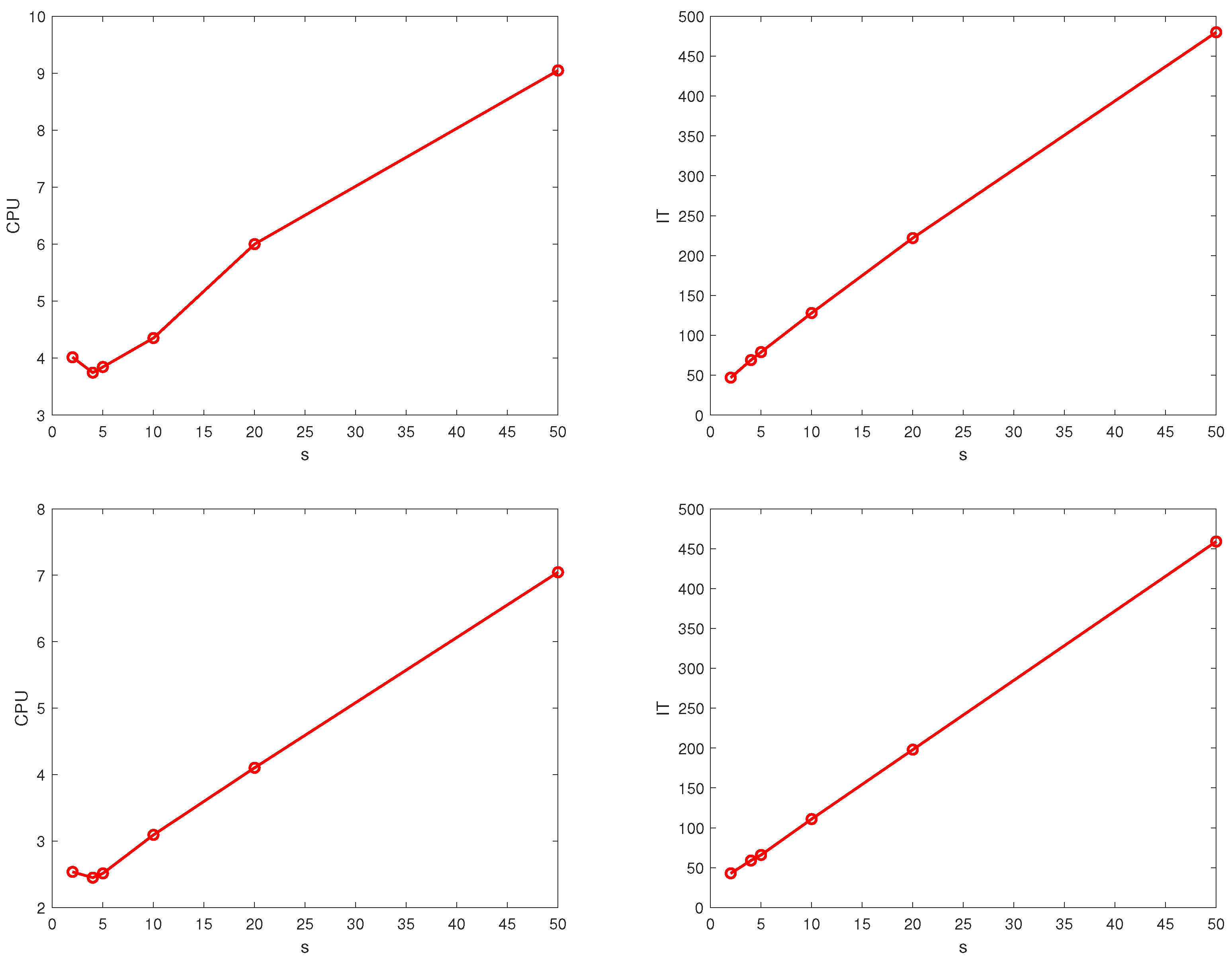
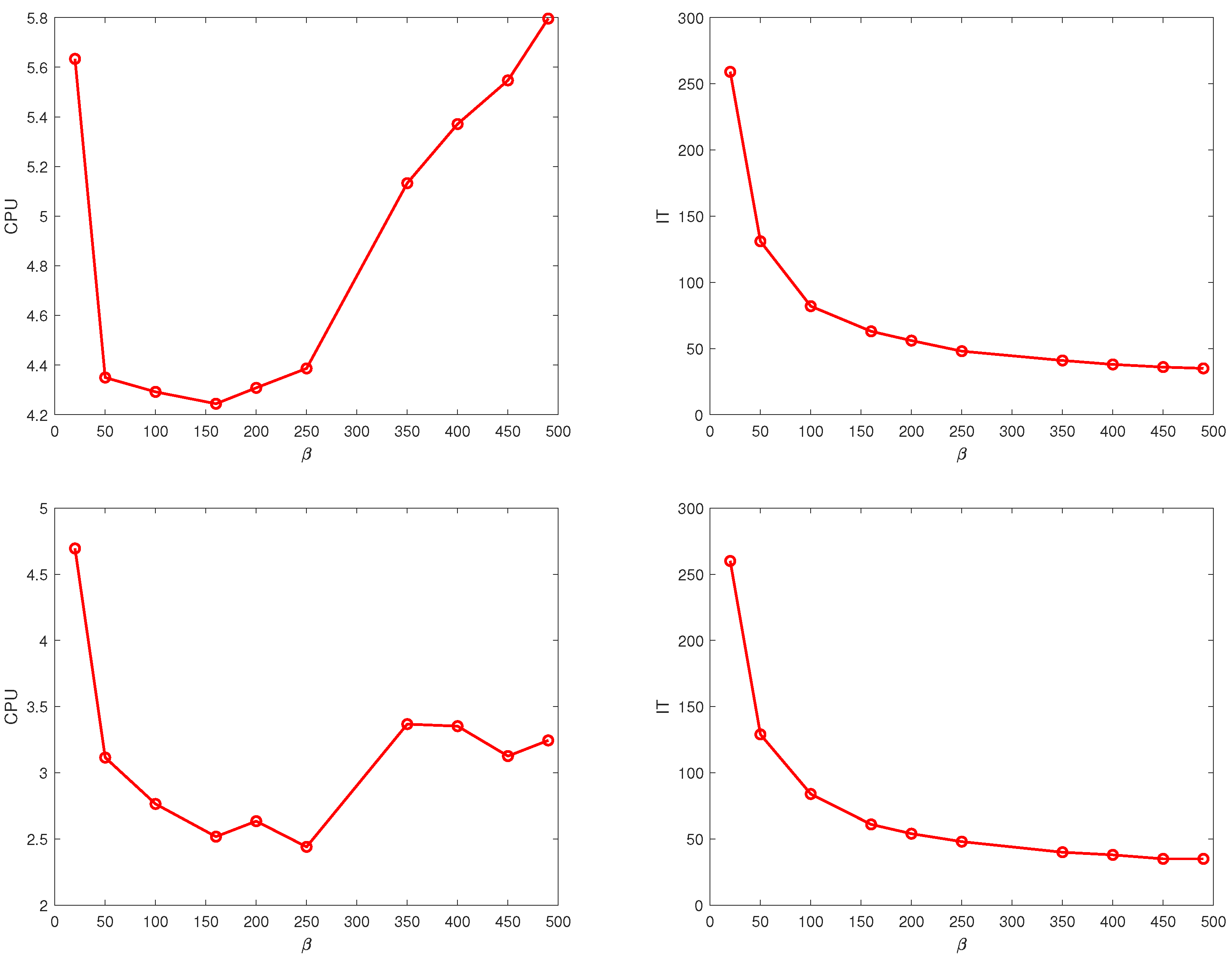
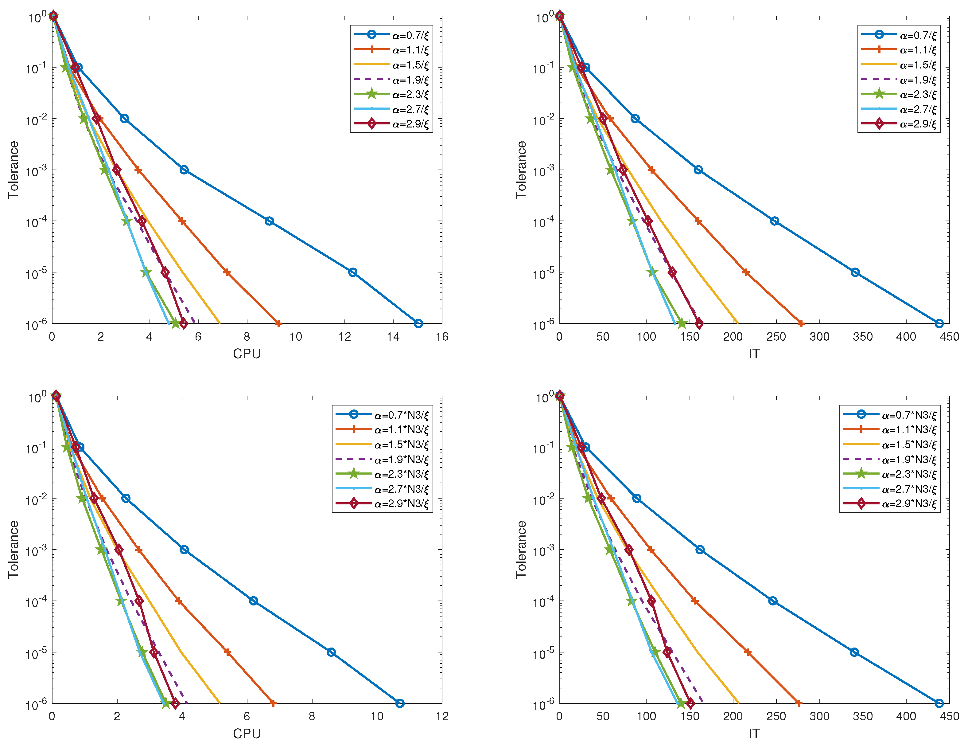
In the TRAK, TRAKS, ${\mathrm{TRAK}}_{\mathrm{F}}$, and ${\mathrm{TRAKS}}_{\mathrm{F}}$ algorithms, we know that s, $\beta$, and $\alpha$ affect the numerical results. Thus, we first show how they impact the performance of our methods in Figure 1, Figure 2, Figure 3 and Figure 4. In Figure 1, we plot the CPU and IT of the TRAK and ${\mathrm{TRAK}}_{\mathrm{F}}$ algorithms with the number of partitions $s=10$ and different stepsizes $\alpha$ for different tolerances. We can find that the convergences of the TRAK and ${\mathrm{TRAK}}_{\mathrm{F}}$ algorithms are quicker with respect to the increase of $\alpha$ and the fixed $s=10$, but slow down after reaching the faster convergence rate. Moreover, the TRAK and ${\mathrm{TRAK}}_{\mathrm{F}}$ algorithms also converge for ${\alpha }_{TRAK}\ge 2/\xi$ and ${\alpha }_{TRA{K}_F}\ge 2N_3/\xi$, and converge much faster by using the appropriate extrapolated stepsize. In Figure 2, we plot the curves of the TRAKS and ${\mathrm{TRAKS}}_{\mathrm{F}}$ algorithms with different stepsizes when $\beta =100$. In this experiment, we approximate ${\xi }_1=\underset{{\tau }_k\subset \left[N_1\right],\left|{\tau }_k\right|=\beta }{max}\frac{\parallel {\mathcal{A}}_{{\tau }_k,:,:}{\parallel }_2^2}{\parallel {\mathcal{A}}_{{\tau }_k,:,:}{\parallel }_F^2}$ by using the maximum value of $\frac{\parallel {\mathcal{A}}_{{\tau }_k,:,:}{\parallel }_2^2}{\parallel {\mathcal{A}}_{{\tau }_k,:,:}{\parallel }_F^2}$ obtained by random sampling 100 times. From this figure, we can observe that the convergence rates of the TRAKS and ${\mathrm{TRAKS}}_{\mathrm{F}}$ algorithms raise firstly and then slow down with respect to the increase of $\alpha$.

Figure 1. CPU and IT of the TRAK and ${\mathrm{TRAK}}_{\mathrm{F}}$ algorithms with the number of partitions $s=10$ and different stepsizes $\alpha$ for different tolerances. Upper: TRAK. Lower: ${\mathrm{TRAK}}_{\mathrm{F}}$.

Figure 2. CPU and IT of the TRAKS and ${\mathrm{TRAKS}}_{\mathrm{F}}$ algorithms with $\beta =100$ and different stepsizes $\alpha$ for different tolerances. Upper: TRAKS. Lower: ${\mathrm{TRAKS}}_{\mathrm{F}}$.

Figure 3. CPU and IT of the TRAK and ${\mathrm{TRAK}}_{\mathrm{F}}$ algorithms with extrapolated stepsize and different number of partitions. Upper: TRAK. Lower: ${\mathrm{TRAK}}_{\mathrm{F}}$.

Figure 4. CPU and IT of the TRAKS and ${\mathrm{TRAKS}}_{\mathrm{F}}$ algorithms for different $\beta$. Upper: TRAKS. Lower: ${\mathrm{TRAKS}}_{\mathrm{F}}$.

In Figure 3, we depict the curves of the average number of iterations and computing times of the TRAK and ${\mathrm{TRAK}}_{\mathrm{F}}$ algorithms versus the different number of partitions. In Figure 4, we plot the curves of the average CPU times and average IT of the TRAKS and ${\mathrm{TRAKS}}_{\mathrm{F}}$ algorithms for different $\beta$. We use ${\alpha }_{TRAKS}=1.95/{\xi }_1$, ${\alpha }_{{\mathrm{TRAKS}}_{\mathrm{F}}}=1.95N_3/{\xi }_1$, ${\alpha }_{TRAK}=1.95/\xi$ and ${\alpha }_{TRA{K}_F}=1.95N_3/\xi$. For all cases, we set $tolerance={10}^{-5}$. From these figures, we see that the CPU times are decreasing at the beginning and then increasing with respect to the increase of parameters. The number of iteration steps are always increasing, with respect to the increase of s, for both TRAK and ${\mathrm{TRAK}}_{\mathrm{F}}$, while the TRAKS and ${\mathrm{TRAKS}}_{\mathrm{F}}$ algorithms are the opposite for the number of iteration steps. In general, from Figure 1, Figure 2, Figure 3 and Figure 4, there is an optimal combination of parameters that makes our algorithms perform best. In the following experiments, we use the optimal experimental results obtained by trial and error.

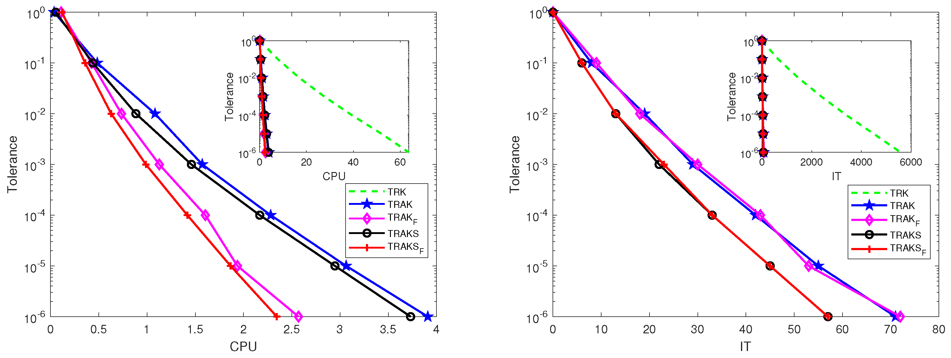
To compare the performances of these algorithms, we use ${\alpha }_{\mathrm{TRK}}=1.3$, which makes the TRK algorithm achieve optimal performance. For the TRAK, ${\mathrm{TRAK}}_{\mathrm{F}}$, TRAKS, and ${\mathrm{TRAKS}}_{\mathrm{F}}$ algorithms, ${\alpha }_{\mathrm{TRAK}}=2.5/\xi$, ${\alpha }_{{\mathrm{TRAK}}_{\mathrm{F}}}=2.5N_3/\xi$, $s_{\mathrm{TRAK}}=s_{{\mathrm{TRAK}}_{\mathrm{F}}}=4$, ${\alpha }_{\mathrm{TRAKS}}=2.7/{\xi }_1$, ${\alpha }_{{\mathrm{TRAKS}}_{\mathrm{F}}}=2.7N_3/{\xi }_1$ and ${\beta }_{\mathrm{TRAKS}}={\beta }_{{\mathrm{TRAKS}}_{\mathrm{F}}}=160$ are used. In Figure 5, we depict the curves of tolerance versus the iteration steps and the calculated times. We observe that the TRAK, ${\mathrm{TRAK}}_{\mathrm{F}}$, TRAKS, and ${\mathrm{TRAKS}}_{\mathrm{F}}$ algorithms converge much faster than the TRK algorithm, and the original algorithms and their Fourier versions have the same number of iteration steps for identical tolerance. The ${\mathrm{TRAKS}}_{\mathrm{F}}$ algorithm has the best performance in terms of CPU time.

Figure 5. Pictures of tolerance versus IT and CPU times for the TRK, TRAK, ${\mathrm{TRAK}}_{\mathrm{F}}$, TRAKS, and ${\mathrm{TRAKS}}_{\mathrm{F}}$ algorithms when $\mathcal{X}$ is synthetic data.

6.2. 3D MRI Image Data

This experiment considers an image data $\mathcal{X}\in {\mathbb{R}}^{128\times 128\times 27}$ from data set mri in MATLAB. We generate randomly a Gaussian tensor $\mathcal{A}\in {\mathbb{R}}^{1000\times 128\times 27}$ and form the measurement tensor $\mathcal{B}$ by $\mathcal{B}=\mathcal{A}\ast \mathcal{X}$. The parameters are tuned to achieve optimal performance in all algorithms. We use ${\alpha }_{TRK}=1.2$, ${\alpha }_{TRAK}=2.3/\xi$, ${\alpha }_{TRA{K}_F}=(2.3N_3)/\xi$, $s_{TRAK}=s_{TRA{K}_F}=4$, ${\alpha }_{TRAKS}=2.4/{\xi }_1$, ${\alpha }_{{\mathrm{TRAKS}}_{\mathrm{F}}}=2.4N_3/{\xi }_1$ and ${\beta }_{\mathrm{TRAKS}}={\beta }_{{\mathrm{TRAKS}}_{\mathrm{F}}}=160$. The results are reported in Figure 6. From the figure, we find that the TRAK, ${\mathrm{TRAK}}_{\mathrm{F}}$, TRAKS, and ${\mathrm{TRAKS}}_{\mathrm{F}}$ algorithms significantly outperform the TRK algorithm. Meanwhile, it is easy to see that the ${\mathrm{TRAKS}}_{\mathrm{F}}$ algorithm performs better than the other algorithms in terms of CPU time.

Figure 6. Pictures of tolerance versus IT and CPU times for the TRK, TRAK, ${\mathrm{TRAK}}_{\mathrm{F}}$, TRAKS, and ${\mathrm{TRAKS}}_{\mathrm{F}}$ algorithms when $\mathcal{X}$ comes from the 3D MRI image data set.

6.3. Video Data

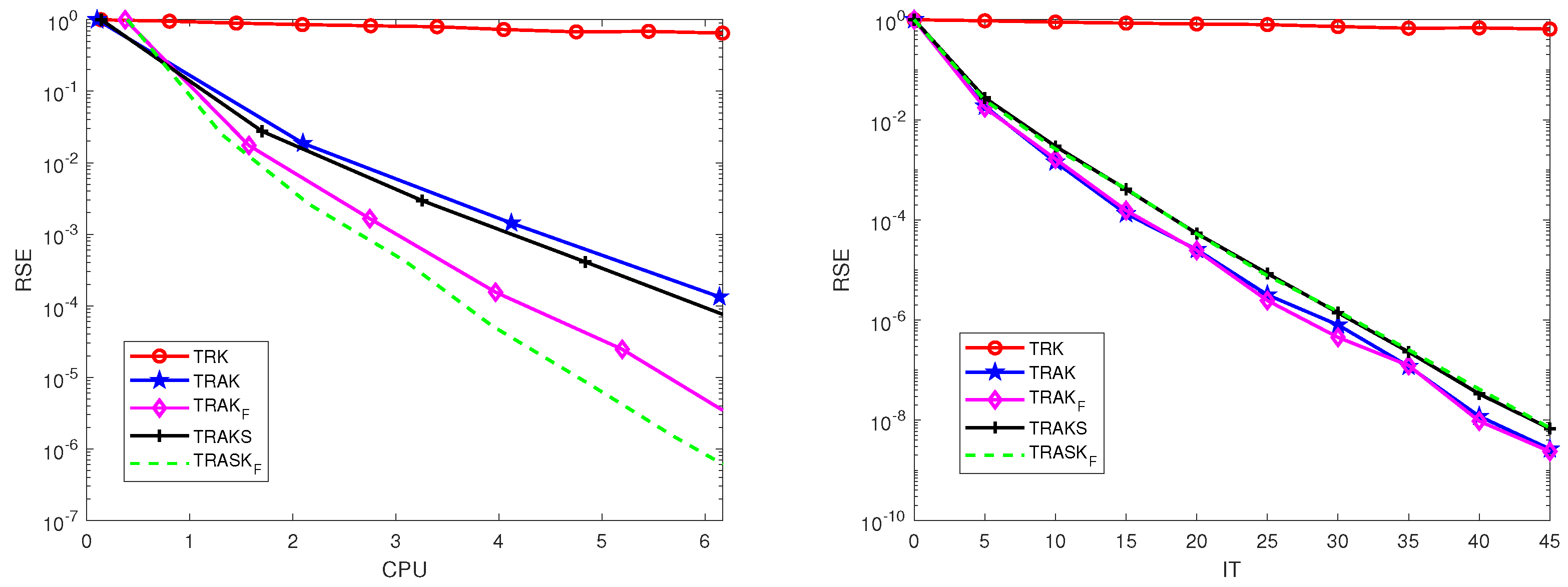
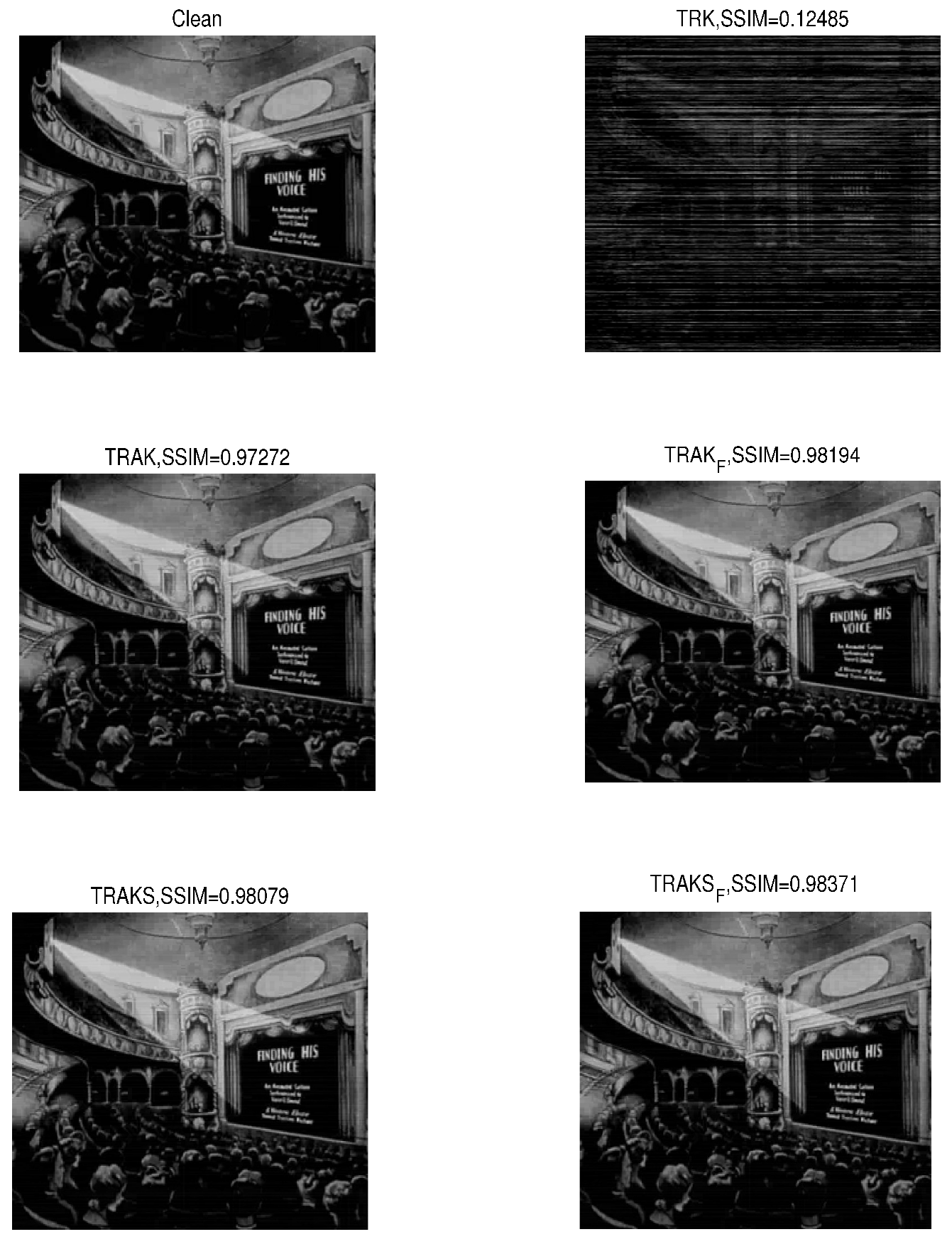
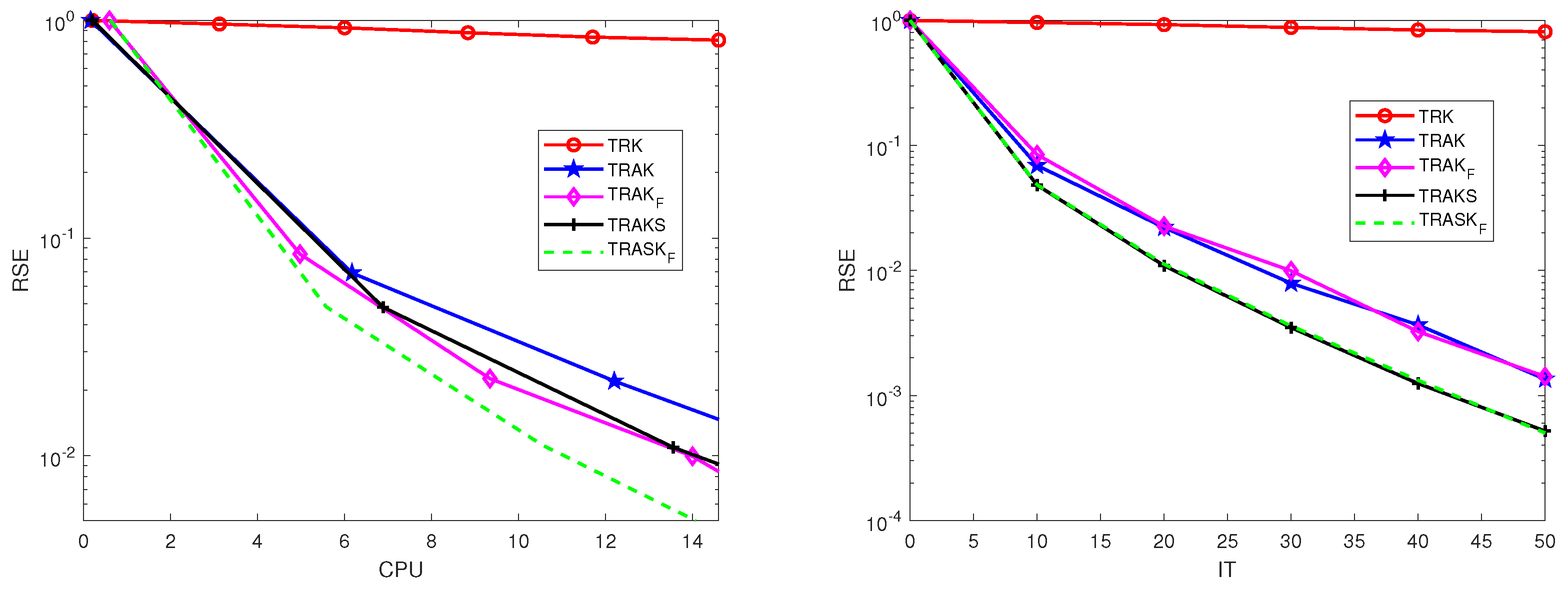
The experiment was implemented on video data, where the frontal slices of tensor $\mathcal{X}$ were the first 60 frames from the 1929 film “Finding His Voice” [25]. Each video frame had $240\times 320$ pixels. Similar to Experiment Section 6.2, we randomly obtained a Gaussian tensor $\mathcal{A}\in {\mathbb{R}}^{1000\times 240\times 60}$ and form the measurement tensor $\mathcal{B}$ by $\mathcal{B}=\mathcal{A}\ast \mathcal{X}$. In this test, we used ${\alpha }_{TRK}=1.3$, ${\alpha }_{TRAK}=2.3/\xi$, ${\alpha }_{TRA{K}_F}=(2.3N_3)/\xi$, $s_{TRAK}=s_{TRA{K}_F}=4$, ${\alpha }_{TRAKS}=2.8/{\xi }_1$, ${\alpha }_{{\mathrm{TRAKS}}_{\mathrm{F}}}=2.8N_3/{\xi }_1$ and ${\beta }_{\mathrm{TRAKS}}={\beta }_{{\mathrm{TRAKS}}_{\mathrm{F}}}=170$, which made all algorithms achieve the best performance. In Figure 7, we plot the curves of the average RSE versus IT and CPU times for all algorithms. From this figure, we observe that the TRAK, ${\mathrm{TRAK}}_{\mathrm{F}}$, TRAKS, and ${\mathrm{TRAKS}}_{\mathrm{F}}$ algorithms significantly outperformed the TRK algorithm in terms of IT and CPU times and the ${\mathrm{TRAKS}}_{\mathrm{F}}$ algorithm had a great advantage in the calculating time. In addition, we run the TRK, TRAK, ${\mathrm{TRAKS}}_{\mathrm{F}}$, TRAKS, and ${\mathrm{TRAKS}}_{\mathrm{F}}$ algorithms for 50, 15, 15, 19, and 19 iterations, respectively. Their reconstructions are reported in Figure 8. From Figure 8, we observe that the SSIM of the TRK algorithm was much smaller than that of the TRAK, ${\mathrm{TRAK}}_{\mathrm{F}}$, TRAKS, and ${\mathrm{TRAKS}}_{\mathrm{F}}$ algorithms, which implies that the reconstruction results of the TRAK, ${\mathrm{TRAK}}_{\mathrm{F}}$, TRAKS, and ${\mathrm{TRAKS}}_{\mathrm{F}}$ algorithms are apparently better than that of the TRK algorithm. Moreover, the ${\mathrm{TRAKS}}_{\mathrm{F}}$ algorithm requires less CPU time than the other algorithms.

Figure 7. Pictures of the average RSE versus IT and CPU times for the TRK, TRAK, ${\mathrm{TRAK}}_{\mathrm{F}}$, TRAKS, and ${\mathrm{TRAKS}}_{\mathrm{F}}$ algorithms when $\mathcal{X}$ is the video datum.

Figure 8. The $50th$ frame of the clean film and the images recovered by the TRK, TRAK, ${\mathrm{TRAK}}_{\mathrm{F}}$, TRAKS, and ${\mathrm{TRAKS}}_{\mathrm{F}}$ algorithms. ${\mathrm{CPU}}_{\mathrm{TRK}}=6.6113$, ${\mathrm{CPU}}_{\mathrm{TRAK}}=6.1381$, ${\mathrm{CPU}}_{{\mathrm{TRAK}}_{\mathrm{F}}}=3.9756$, ${\mathrm{CPU}}_{\mathrm{TRAKS}}=6.0760$, ${\mathrm{CPU}}_{{\mathrm{TRAKS}}_{\mathrm{F}}}=3.8270$.

6.4. CT Data

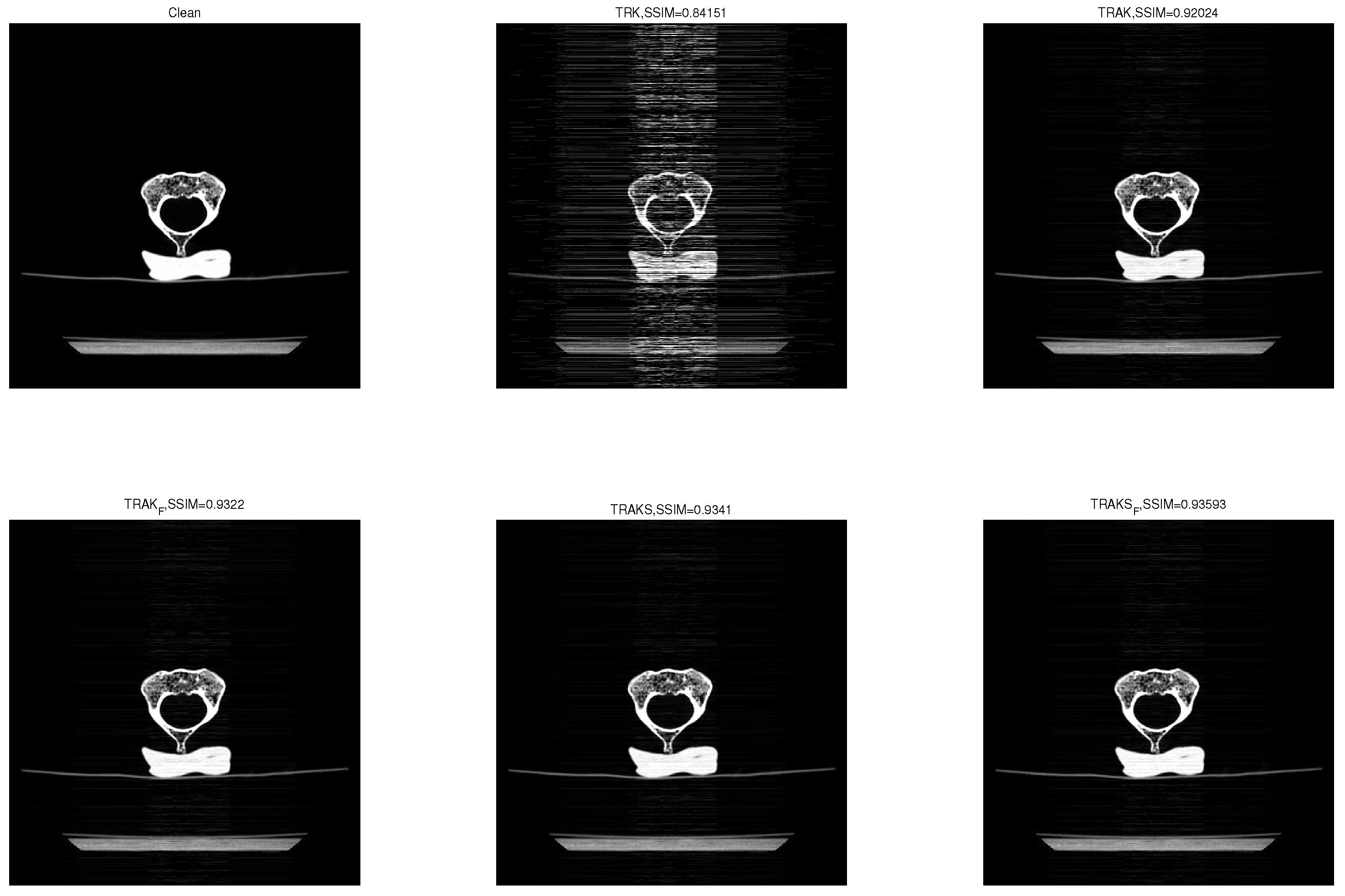
In this experiment, we test the performance of the algorithms using the real world CT data set. The underlying signal $\mathcal{X}$ is a tensor of size $512\times 512\times 42$, where each frontal slice is a $512\times 512$ matrix of the C2-vertebrae. The images were taken from the Laboratory of the Human Anatomy and Embryology, University of Brussels (ULB), Belgium [26]. We also obtain randomly a Gaussian tensor $\mathcal{A}\in {\mathbb{R}}^{1000\times 512\times 42}$ and $\mathcal{B}=\mathcal{A}\ast \mathcal{X}$. Let ${\alpha }_{TRK}=1.3$, ${\alpha }_{TRAK}=2.3/\xi$, ${\alpha }_{TRA{K}_F}=(2.3N_3)/\xi$, $s_{TRAK}=s_{TRA{K}_F}=5$, ${\alpha }_{TRAKS}=2.6/{\xi }_1$, ${\alpha }_{{\mathrm{TRAKS}}_{\mathrm{F}}}=2.6N_3/{\xi }_1$ and ${\beta }_{\mathrm{TRAKS}}={\beta }_{{\mathrm{TRAKS}}_{\mathrm{F}}}=250$. We run the TRK, TRAK, ${\mathrm{TRAK}}_{\mathrm{F}}$, TRAKS, and ${\mathrm{TRAKS}}_{\mathrm{F}}$ algorithms for 40, 15, 15, 13, and 13 iterations, respectively. Their numerical results are presented in Figure 9 and Figure 10. From Figure 9, we see again that the TRAK, ${\mathrm{TRAK}}_{\mathrm{F}}$, TRAKS, and ${\mathrm{TRAKS}}_{\mathrm{F}}$ algorithms converge faster than the TRK algorithm. From Figure 10, we observe that the SSIMs of the TRAK, ${\mathrm{TRAK}}_{\mathrm{F}}$, TRAKS, and ${\mathrm{TRAKS}}_{\mathrm{F}}$ algorithms are much closer to 1 than that of the TRK algorithm, which implies that the TRAK, ${\mathrm{TRAK}}_{\mathrm{F}}$, TRAKS, and ${\mathrm{TRAKS}}_{\mathrm{F}}$ algorithms achieve better reconstruction results. In addition, the ${\mathrm{TRAKS}}_{\mathrm{F}}$ algorithm requires less CPU time than the other algorithms.

Figure 9. Pictures of the average RSE versus IT and CPU times for the TRK, TRAK, ${\mathrm{TRAK}}_{\mathrm{F}}$, TRAKS, and ${\mathrm{TRAKS}}_{\mathrm{F}}$ algorithms when $\mathcal{X}$ is a CT data.

Figure 10. The $39th$ slice of the clean image sequence and the images recovered by the TRK, TRAK, ${\mathrm{TRAK}}_{\mathrm{F}}$ algorithms. ${\mathrm{CPU}}_{\mathrm{TRK}}=12.0177$, ${\mathrm{CPU}}_{\mathrm{TRAK}}=9.3976$, ${\mathrm{CPU}}_{{\mathrm{TRAK}}_{\mathrm{F}}}=7.5307$, ${\mathrm{CPU}}_{\mathrm{TRAKS}}=9.2294$, ${\mathrm{CPU}}_{{\mathrm{TRAKS}}_{\mathrm{F}}}=7.3547$.

7. Conclusions

In this paper, we propose the TRAK and TRAKS algorithms and discuss the Fourier domain version. The new algorithms can be efficiently implemented in distributed computing units. Numerical results show that the new algorithms have better performance than the TRK algorithm. Meanwhile, we note that the sizes of the samples, the number of partitions, and the stepsizes play important roles in guaranteeing fast convergences of the new methods. Therefore, in future work, we will obtain more appropriate parameters.

References

- Kilmer, M.E.; Martin, C.D. Factorization strategies for third-order tensors. Linear Algebra Its Appl. 2011, 435, 641–658. [Google Scholar] [CrossRef]
- Newman, E.; Horesh, L.; Avron, H.; Kilmer, M. Stable tensor neural networks for rapid deep learning. arXiv 2018, arXiv:1811.06569. [Google Scholar]
- Soltani, S.; Kilmer, M.E.; Hansen, P.C. A tensor-based dictionary learning approach to tomographic image reconstruction. Bit Numer. Math. 2016, 56, 1425–1454. [Google Scholar] [CrossRef]
- Hua, Z.; Li, L.; Zhu, H. Tensor regression with applications in neuroimaging data analysis. J. Am. Stat. Assoc. 2013, 108, 540–552. [Google Scholar]
- Andersen, A.H.; Kak, A.C. Simultaneous algebraic reconstruction technique (SART): A superior implementation of the ART algorithm. Ultrason. Imaging 1984, 6, 81–94. [Google Scholar] [CrossRef] [PubMed]
- Peterson, J.E.; Paulsson, B.N.; McEvilly, T.V. Applications of algebraic reconstruction techniques to crosshole seismic data. Geophysics 1985, 50, 1566–1580. [Google Scholar] [CrossRef]
- Zouzias, A.; Freris, N.M. Randomized extended Kaczmarz for solving least squares. SIAM J. Matrix Anal. Appl. 2013, 34, 773–793. [Google Scholar] [CrossRef]
- Needell, D. Randomized Kaczmarz solver for noisy linear systems. BIT Numer. Math. 2010, 50, 395–403. [Google Scholar] [CrossRef]
- Moorman, J.D.; Tu, T.K.; Molitor, D.; Needell, D. Randomized Kaczmarz with averaging. Bit Numer. Math. 2021, 61, 337–359. [Google Scholar] [CrossRef]
- Necoara, I. Faster randomized block Kaczmarz algorithms. SIAM J. Matrix Anal. Appl. 2019, 40, 1425–1452. [Google Scholar] [CrossRef]
- Miao, C.Q.; Wu, W.T. On greedy randomized average block Kaczmarz method for solving large linear systems. J. Comput. Appl. Math. 2022, 413, 114372. [Google Scholar] [CrossRef]
- Elfving, T. Block-iterative methods for consistent and inconsistent linear equations. Numer. Math. 1980, 35, 1–12. [Google Scholar] [CrossRef]
- Eggermont, P.P.B.; Herman, G.T.; Lent, A. Iterative algorithms for large partitioned linear systems with applications to image reconstruction. Linear Algebra Its Appl. 1981, 40, 37–67. [Google Scholar] [CrossRef]
- Needell, D.; Tropp, J.A. Paved with good intentions: Analysis of a randomized block Kaczmarz method. Linear Algebra Its Appl. 2014, 441, 199–221. [Google Scholar] [CrossRef]
- Ma, A.; Molitor, D. Randomized Kaczmarz for tensor linear systems. BIT Numer. Math. 2022, 62, 171–194. [Google Scholar] [CrossRef]
- Tang, L.; Yu, Y.; Zhang, Y.; Li, H. Sketch-and-project methods for tensor linear systems. arXiv 2022, arXiv:2201.00667. [Google Scholar] [CrossRef]
- Chen, X.; Qin, J. Regularized Kaczmarz algorithms for tensor recovery. SIAM J. Imaging Sci. 2021, 14, 1439–1471. [Google Scholar] [CrossRef]
- Wang, X.; Che, M.; Mo, C.; Wei, Y. Solving the system of nonsingular tensor equations via randomized Kaczmarz-like method. J. Comput. Appl. Math. 2023, 421, 114856. [Google Scholar] [CrossRef]
- Kilmer, M.E.; Braman, K.; Hao, N.; Hoover, R.C. Third-order tensors as operators on matrices: A theoretical and computational framework with applications in imaging. SIAM J. Matrix Anal. Appl. 2013, 34, 148–172. [Google Scholar] [CrossRef]
- Jin, H.; Bai, M.; Benítez, J.; Liu, X. The generalized inverses of tensors and an application to linear models. Comput. Math. Appl. 2017, 74, 385–397. [Google Scholar] [CrossRef]
- Jiang, Y.; Wu, G.; Jiang, L. A Kaczmarz method with simple random sampling for solving large linear systems. arXiv 2020, arXiv:2011.14693. [Google Scholar]
- Carlton, M.A. Probability and Statistics for Computer Scientists. Am. Stat. 2008, 62, 271–272. [Google Scholar] [CrossRef]
- Wang, Q.; Li, W.; Bao, W.; Gao, X. Nonlinear Kaczmarz algorithms and their convergence. J. Comput. Appl. Math. 2022, 399, 113720. [Google Scholar] [CrossRef]
- Lu, C. Tensor-Tensor Product Toolbox. Carnegie Mellon University. 2018. Available online: https://github.com/canyilu/tproduct (accessed on 17 July 2022).
- Finding His Voice. Available online: https://archive.org/details/FindingH1929 (accessed on 15 August 2022).
- Bone and Joint ct-scan Data. Available online: https://isbweb.org/data/vsj/ (accessed on 25 August 2022).
Publisher’s Note: MDPI stays neutral with regard to jurisdictional claims in published maps and institutional affiliations. |
© 2022 by the authors. Licensee MDPI, Basel, Switzerland. This article is an open access article distributed under the terms and conditions of the Creative Commons Attribution (CC BY) license (https://creativecommons.org/licenses/by/4.0/).