A Polynomial Fitting Problem: The Orthogonal Distances Method

Abstract

The classical curve-fitting problem to relate two variables, x and y, deals with polynomials. Generally, this problem is solved by the least squares method (LS), where the minimization function considers the vertical errors from the data points to the fitting curve. Another curve-fitting method is total least squares (TLS), which takes into account errors in both x and y variables. A further method is the orthogonal distances method (OD), which minimizes the sum of the squares of orthogonal distances from the data points to the fitting curve. In this work, we develop the OD method for the polynomial fitting of degree n and compare the TLS and OD methods. The results show that TLS and OD methods are not equivalent in general; however, both methods get the same estimates when a polynomial of degree 1 without an independent coefficient is considered. As examples, we consider the calibration curve-fitting problem of a R-type thermocouple by polynomials of degrees 1 to 4, with and without an independent coefficient, using the LS, TLS and OD methods.

1. Introduction

The curve-fitting or parameter estimation procedure consists of determining the parameters of a curve to obtain the best possible fit to observations. Depending on the curve, this problem can be classified as linear or nonlinear [1,2]. The most used curves for fitting in biology, physics, statistics and engineering are polynomials $y=a_0+a_{1}x+\cdots +a_{n-1}{x}^{n-1}+a_n{x}^n$ [3,4,5,6,7]. The polynomial fitting is a linear problem and the most popular method used to solve it is least squares (LS) [8,9,10], which minimizes the sum of the squares of vertical errors from the data points $(x_1,y_1),\dots ,(x_m,y_m)$ to the polynomial curve. Another method that can be used to solve the problem is total least squares (TLS), which considers that both x and y are subject to errors; this method was developed mainly by Golub and Van Loan [11] and Van Huffel and Vandewalle [12]; however, the consideration that both variables x and y are subject to errors dates back at least to 1943 in the work of Deming [13]. Another way to solve the polynomial fitting is to consider the minimization of the sum of the squares of orthogonal distances from the data points to the polynomial curve, called in this article as the orthogonal distances (OD) method. Adcock [14] was the first to use the OD method for the straight line fitting; however, it has also been studied and used for the straight line and planes fitting in [15,16,17,18,19,20,21].

The remainder of this paper is structured as follows: Section 2 presents a brief description of the LS and TLS methods. The OD method is developed in Section 3 and it is also compared with the TLS method using the polynomial of degree 1. The approximation of the output voltage corresponding to different temperatures of a R-type thermocouple [22] using polynomials of degrees 1 to 4 by LS, TLS and OD methods is carried out in Section 4. Finally, a discussion and concluding remarks are presented in Section 5 and Section 6, respectively.

In general, this article studies the polynomial fitting problem by the OD method, and the main contributions are the following:

• Development of the OD method for polynomial fitting of degree n.
• Polynomial fitting of thermoelectric voltage data from a R-type thermocouple by OD, LS and TLS methods.
• From the numerical experiments studied, the TLS and OD methods are not equivalent in general. However, both methods obtain the same estimates when the polynomial of degree 1 without an independent coefficient is used.

2. Polynomial Fitting by LS and TLS Methods

The polynomial fitting of degree n consists of determining the unknown parameters $a_0,a_1,\dots ,a_n$ of the polynomial defined for all real numbers x, such that $f(x)=a_0+a_{1}x+\cdots +a_{n-1}{x}^{n-1}+a_n{x}^n$. A brief description of the LS and TLS solutions for polynomial fitting are presented below.

2.1. The LS Method

The LS method is one of the most widely used minimization criteria for parameter estimation. The first publication of the method was made by A. M. Legendre in 1805; however, C. F. Gauss claimed that he used the method 10 years earlier [16]. The classical LS method seeks to determine the curve $y=f(x)$, which best fits to observations $(x_i,y_i)$ with $i=1,\dots ,m$, minimizing the sum of the squares of vertical errors defined as $r_i=y_i-f(x_i)$; however, there are some variants of the method, such as weighted least squares, generalized least squares and maximum likelihood, among others, and it can be applied to different mathematical models, such as algebraic models, and continuous and discrete dynamic models [23,24,25,26,27,28] using the off-line and recursive schemes [20,29,30].

Since the article considers the classical LS method under the off-line scheme, the vector of vertical errors for the polynomial of degree n and observations $(x_i,y_i)$ is given by

$$\begin{array}{c}\hfill \mathbf{r}=\left[\begin{array}{c}{r}_1\\ r_2\\ ⋮\\ r_m\end{array}\right]=\left[\begin{array}{c}{y}_1\\ y_2\\ ⋮\\ y_m\end{array}\right]-\left[\begin{array}{cccc}1& x_1& \cdots & x_1^n\\ 1& x_2& \cdots & x_2^n\\ ⋮& ⋮& & ⋮\\ 1& x_m& \cdots & x_m^n\end{array}\right]\left[\begin{array}{c}{a}_0\\ a_1\\ ⋮\\ a_n\end{array}\right].\end{array}$$

Defining

$$\begin{array}{c}\hfill \mathbf{y}:=\left[\begin{array}{c}{y}_1\\ y_2\\ ⋮\\ y_m\end{array}\right],\mathbf{A}:=\left[\begin{array}{cccc}1& x_1& \cdots & x_1^n\\ 1& x_2& \cdots & x_2^n\\ ⋮& ⋮& & ⋮\\ 1& x_m& \cdots & x_m^n\end{array}\right],\mathbf{p}:=\left[\begin{array}{c}{a}_0\\ a_1\\ ⋮\\ a_n\end{array}\right],\end{array}$$

we obtain

$$\begin{array}{c}\hfill \mathbf{r}=\mathbf{y}-\mathbf{Ap},\end{array}$$

(1)

where $\mathbf{A}\in {\mathbb{R}}^{m\times (n+1)}$, $\mathbf{y}\in {\mathbb{R}}^m$ and $\mathbf{p}\in {\mathbb{R}}^{(n+1)}$.

Taking the squared 2-norm of vector (1), we obtain

$$\begin{array}{c}\hfill \parallel \mathbf{r}{\parallel }_2^2=\parallel \mathbf{y}-\mathbf{Ap}{\parallel }_2^2=\sum _{i=1}^m{r}_i^2.\end{array}$$

(2)

The LS solution is the vector $\mathbf{p}$ such that it minimizes the functional (2). Since it is a linear minimization problem, the LS solution can be found by elementary calculus [10,31,32]. The $\mathbf{p}$ LS solution which minimizes (2) is unique if matrix $\mathbf{A}$ has independent columns, which means that it has rank $\rho (\mathbf{A})=n+1$. Therefore, the $\mathbf{p}$ LS solution satisfies the normal equations ${\mathbf{A}}^{\top }\mathbf{Ap}={\mathbf{A}}^{\top }\mathbf{y}$ and is defined by $\mathbf{p}={({\mathbf{A}}^{\top }\mathbf{A})}^{-1}{\mathbf{A}}^{\top }\mathbf{y}$.

On the other hand, if matrix $\mathbf{A}$ has dependent columns or is not invertible, the $\mathbf{p}$ LS solution which minimizes (2) is defined by

$$\begin{array}{c}\hfill \mathbf{p}={\mathbf{A}}^{†}\mathbf{y},\end{array}$$

(3)

where ${\mathbf{A}}^{†}$ is called the Moore–Penrose pseudoinverse of $\mathbf{A}$, and it is defined by

$$\begin{array}{c}\hfill {\mathbf{A}}^{†}=V\left[\begin{array}{cc}{\Sigma }_q^{-1}& \mathbf{0}\\ \mathbf{0}& \mathbf{0}\end{array}\right]U^{\top }.\end{array}$$

Equation (3) is called the pseudoinverse solution of the LS method, and the Moore–Penrose pseudoinverse is defined by the matrices of the singular value decomposition (SVD) given by the following theorem. Throughout the text, the rank of any matrix will be denoted by $\rho (·)$.

Theorem 1.

([10]). Let any matrix $\mathbf{A}\in {\mathbb{R}}^{m\times (n+1)}$. The SVD of $\mathbf{A}$ is

$$\begin{array}{c}\hfill \mathbf{A}=U\left[\begin{array}{cc}{\Sigma }_q& \mathbf{0}\\ \mathbf{0}& \mathbf{0}\end{array}\right]V^{\top },\end{array}$$

where $U\in {\mathbb{R}}^{m\times m}$ and $V\in {\mathbb{R}}^{(n+1)\times (n+1)}$ are unitary matrices and ${\Sigma }_q=diag({\sigma }_1,{\sigma }_2,\cdots ,{\sigma }_q)$. The numbers ${\sigma }_1\ge {\sigma }_2\ge \cdots \ge {\sigma }_q>0$ are called the singular values of $\mathbf{A}$ and $\rho (\mathbf{A})=q$.

More properties of the Moore–Penrose pseudoinverse can be found in [10,32].

2.2. The TLS Method

This section presents the most important results of the TLS method from [12] for polynomial fitting.

Rewriting the system of linear algebraic equations $\mathbf{Ap}=\mathbf{y}$ as follows

$$\begin{array}{c}\hfill \left[\begin{array}{cc}\mathbf{A}& \mathbf{y}\end{array}\right]\left[\begin{array}{c}\mathbf{p}\\ -1\end{array}\right]=\mathbf{0},\end{array}$$

since $\mathbf{A}\in {\mathbb{R}}^{m\times (n+1)}$, $\mathbf{y}\in {\mathbb{R}}^m$ and $\mathbf{p}\in {\mathbb{R}}^{(n+1)}$, it can be defined $\mathbf{\Lambda }\mathbf{:}\mathbf{=}\left[\begin{array}{cc}\mathbf{A}& \mathbf{y}\end{array}\right]\in {\mathbb{R}}^{m\times (n+2)}$ and $\mathbf{z}:=\left[\begin{array}{c}\mathbf{p}\\ -1\end{array}\right]\in {\mathbb{R}}^{(n+2)}$ to obtain

$$\begin{array}{c}\hfill \mathbf{\Lambda }\mathbf{z}=\mathbf{0}.\end{array}$$

(4)

Since Equation (4) represents a homogeneous system of linear algebraic equations, the $\mathbf{z}$ solution is in the null space of $\mathbf{\Lambda }$, which means that the parameters vector $\mathbf{p}$ is also in the null space of $\mathbf{\Lambda }$. If matrix $\mathbf{\Lambda }$ in (4) has rank $\rho (\mathbf{\Lambda })=n+2$, the SVD of $\mathbf{\Lambda }$ is given by

$$\begin{array}{c}\hfill \mathbf{\Lambda }=U\Sigma V^{\top }=\sum _{i=1}^{n+2}{\sigma }_i{\mathbf{u}}_i{\mathbf{v}}_i^{\top },\end{array}$$

where the singular values ${\sigma }_i$ and singular vectors ${\mathbf{u}}_i$ and ${\mathbf{v}}_i$ satisfy

$$\begin{array}{ccc}\hfill \mathbf{\Lambda }{\mathbf{v}}_1& =& \hfill {\sigma }_1{\mathbf{u}}_1,\hfill \\ \hfill \mathbf{\Lambda }{\mathbf{v}}_2& =& \hfill {\sigma }_2{\mathbf{u}}_2,\hfill \\ & ⋮& \hfill \hfill \\ \hfill \mathbf{\Lambda }{\mathbf{v}}_{n+1}& =& \hfill {\sigma }_{n+1}{\mathbf{u}}_{n+1},\hfill \\ \hfill \mathbf{\Lambda }{\mathbf{v}}_{n+2}& =& \hfill {\sigma }_{n+2}{\mathbf{u}}_{n+2}.\hfill \end{array}$$

(5)

From (5), it can be see that system (4) does not have a vector $\mathbf{v}$ in the null space of $\mathbf{\Lambda }$, and therefore the TLS method searches for a matrix ${\mathbf{\Lambda }}_k$ with $\rho ({\mathbf{\Lambda }}_k)=k<n+2$, such that $\parallel \mathbf{\Lambda }-{\mathbf{\Lambda }}_k\parallel$ is minimal. Once a minimizing ${\mathbf{\Lambda }}_k$ is found, any $\mathbf{z}$ vector satisfying ${\mathbf{\Lambda }}_k\mathbf{z}=\mathbf{0}$ is called the TLS solution and $\Delta \mathbf{\Lambda }=\mathbf{\Lambda }-{\mathbf{\Lambda }}_k$ is the TLS correction.

The minimization is found by the Eckart–Young–Mirsky theorem. This theorem was initially proved by Eckart and Young [33] using the Frobenius norm, and later Mirsky [34] proved it using the 2-norm. In this work, it is used with the 2-norm. The Eckart–Young–Mirsky theorem using the 2-norm is presented below.

Theorem 2.

([12]). Let the SVD of $\mathbf{\Lambda }\in {\mathbb{R}}^{m\times (n+2)}$ be given by $\mathbf{\Lambda }=U\Sigma V^{\top }$ with $\rho (\mathbf{\Lambda })=q$ and let $k<q$; then, the matrix

$$\begin{array}{c}\hfill {\mathbf{\Lambda }}_k=\sum _{i=1}^k{\sigma }_i{\mathbf{u}}_i{\mathbf{v}}_i^{\top },\end{array}$$

satisfies

$$\begin{array}{c}\hfill \underset{\rho (\mathbf{\Lambda })=k}{\min }\parallel \mathbf{\Lambda }-\mathbf{B}{\parallel }_2=\parallel \mathbf{\Lambda }-{\mathbf{\Lambda }}_k{\parallel }_2={\sigma }_{k+1}.\end{array}$$

Applying the Eckart–Young–Mirsky Theorem 2 to (4), the best matrix approximation ${\mathbf{\Lambda }}_k$ to the matrix $\mathbf{\Lambda }$ is given by

$$\begin{array}{cc}\hfill {\mathbf{\Lambda }}_k=\sum _{i=1}^{n+1}{\sigma }_i{\mathbf{u}}_i{\mathbf{v}}_i^{\top },& {\sigma }_1\ge \cdots \ge {\sigma }_{n+1}>0.\end{array}$$

Notice that ${\mathbf{\Lambda }}_k$ has rank $\rho ({\mathbf{\Lambda }}_k)=n+1$, then the singular values ${\sigma }_i$ and singular vectors ${\mathbf{u}}_i$, ${\mathbf{v}}_i$ now satisfy

$$\begin{array}{ccc}\hfill {\mathbf{\Lambda }}_k{\mathbf{v}}_1& =& \hfill {\sigma }_1{\mathbf{u}}_1,\hfill \\ \hfill {\mathbf{\Lambda }}_k{\mathbf{v}}_2& =& \hfill {\sigma }_2{\mathbf{u}}_2,\hfill \\ & ⋮& \hfill \hfill \\ \hfill {\mathbf{\Lambda }}_k{\mathbf{v}}_{n+1}& =& \hfill {\sigma }_{n+1}{\mathbf{u}}_{n+1},\hfill \\ \hfill {\mathbf{\Lambda }}_k{\mathbf{v}}_{n+2}& =& \hfill 0.\hfill \end{array}$$

(6)

From Equation (6), the vector ${\mathbf{v}}_{n+2}$ is in the null space of ${\mathbf{\Lambda }}_k$, and therefore, a $\mathbf{z}$ TLS solution satisfying ${\mathbf{\Lambda }}_k\mathbf{z}=\mathbf{0}$ is given by

$$\begin{array}{c}\hfill \mathbf{z}=\left[\begin{array}{c}\mathbf{p}\\ -1\end{array}\right]={\mathbf{v}}_{n+2}=\left[\begin{array}{c}{\mathbf{v}}_{1,n+2}\\ {\mathbf{v}}_{2,n+2}\\ ⋮\\ {\mathbf{v}}_{n+2,n+2}\end{array}\right].\end{array}$$

(7)

The TLS solution will be scaled to obtain $-1$ in the last row of (7):

$$\begin{array}{c}\hfill \mathbf{z}=\left[\begin{array}{c}\mathbf{p}\\ -1\end{array}\right]=-\frac{1}{{\mathbf{v}}_{n+2,n+2}}\left[\begin{array}{c}{\mathbf{v}}_{1,n+2}\\ {\mathbf{v}}_{2,n+2}\\ ⋮\\ {\mathbf{v}}_{n+2,n+2}\end{array}\right],\end{array}$$

then, if ${\mathbf{v}}_{n+2,n+2}\ne 0$, the parameters vector $\mathbf{p}$ is given by

$$\begin{array}{c}\hfill \mathbf{p}=-\frac{1}{{\mathbf{v}}_{n+2,n+2}}\left[\begin{array}{c}{\mathbf{v}}_{1,n+2}\\ {\mathbf{v}}_{2,n+2}\\ ⋮\\ {\mathbf{v}}_{n+1,n+2}\end{array}\right].\end{array}$$

(8)

An alternative form to obtain (8) is as follows. Since the $\mathbf{z}$ solution is also an eigenvector of ${\mathbf{\Lambda }}^{\top }\mathbf{\Lambda }$, it is associated with the eigenvalue ${\sigma }_{n+2}^2$. Hence the eigenvalue–eigenvector equation is given by

$$\begin{array}{c}\hfill {\mathbf{\Lambda }}^{\top }\mathbf{\Lambda }\left[\begin{array}{c}\mathbf{p}\\ -1\end{array}\right]={\sigma }_{n+2}^2\left[\begin{array}{c}\mathbf{p}\\ -1\end{array}\right],\end{array}$$

substituting $\mathbf{\Lambda }:=\left[\begin{array}{cc}\mathbf{A}& \mathbf{y}\end{array}\right]$ we obtain

$$\begin{array}{c}\hfill \left[\begin{array}{cc}{\mathbf{A}}^{\top }\mathbf{A}& {\mathbf{A}}^{\top }\mathbf{y}\\ {\mathbf{y}}^{\top }\mathbf{A}& {\mathbf{y}}^{\top }\mathbf{y}\end{array}\right]\left[\begin{array}{c}\mathbf{p}\\ -1\end{array}\right]={\sigma }_{n+2}^2\left[\begin{array}{c}\mathbf{p}\\ -1\end{array}\right].\end{array}$$

(9)

Selecting the first row of Equation (9)

$$\begin{array}{c}\hfill {\mathbf{A}}^{\top }\mathbf{A}\mathbf{p}-{\mathbf{A}}^{\top }\mathbf{y}={\sigma }_{n+2}^2\mathbf{p},\end{array}$$

and solving for the parameters vector $\mathbf{p}$, we obtain

$$\begin{array}{c}\hfill \mathbf{p}={({\mathbf{A}}^{\top }\mathbf{A}-{\sigma }_{n+2}^2\mathbf{I})}^{-1}{\mathbf{A}}^{\top }\mathbf{y}.\end{array}$$

(10)

The following theorem establishes the uniqueness and existence conditions of the TLS solution.

Theorem 3.

([12]). Let the singular values of $\mathbf{A}$ be ${\widehat{\sigma }}_1\ge {\widehat{\sigma }}_2\ge \cdots \ge {\widehat{\sigma }}_{n+1}>0$, and the singular values of $\left[\begin{array}{cc}\mathbf{A}& \mathbf{y}\end{array}\right]$ be ${\sigma }_1\ge {\sigma }_2\ge \cdots \ge {\sigma }_{n+2}>0$. If ${\widehat{\sigma }}_{n+1}>{\sigma }_{n+2}$ then the TLS problem has a unique solution.

As we can see, one problem of the TLS solution is the loss of uniqueness due to repeated singular values, and another is the indeterminate form in (8) if ${\mathbf{v}}_{n+2,n+2}=0$; those problems are called nongeneric TLS problems, and more details of them can be found in [35,36,37].

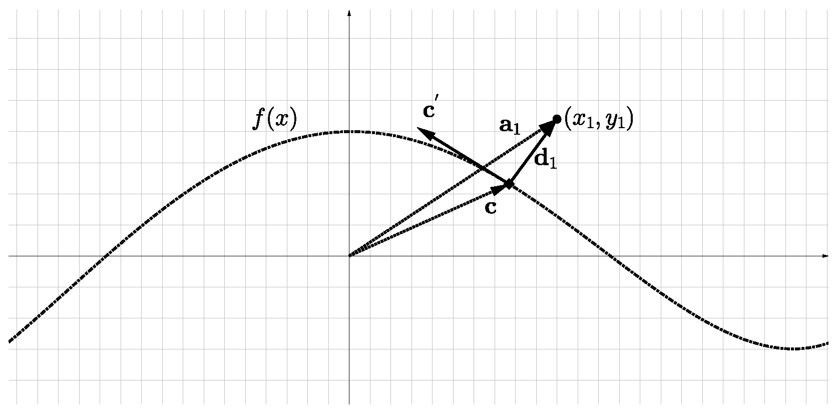
3. Polynomial Fitting by OD Method

The OD method minimizes the sum of the squares of the orthogonal distances from observations $(x_1,y_1),\dots ,(x_m,y_m)$ to the polynomial curve $y=f(x)$. Considering Figure 1, where ${\mathbf{a}}_1$ is the vector of the observation $(x_1,y_1)$, $\mathbf{c}$ is a vector on the curve $\left(x,f(x)\right)$, ${\mathbf{c}}^{{}^{\prime }}:={\displaystyle \frac{\mathrm{d}}{\mathrm{d}x}}\mathbf{c}=\left(1,f^{{}^{\prime }}(x)\right)$ is the tangent vector at $\mathbf{c}$ and the vector ${\mathbf{d}}_1$ is defined by

$$\begin{array}{c}\hfill {\mathbf{d}}_1={\mathbf{a}}_1-\mathbf{c}.\end{array}$$

(11)

The vector ${\mathbf{d}}_1$ in Figure 1 is orthogonal to the curve $f(x)$ at $\mathbf{c}$ if the dot product between vectors ${\mathbf{d}}_1$ and ${\mathbf{c}}^{{}^{\prime }}$ satisfies

$$\begin{array}{c}\hfill {\mathbf{d}}_1·{\mathbf{c}}^{{}^{\prime }}=0.\end{array}$$

(12)

Substituting ${\mathbf{c}}^{{}^{\prime }}$ and ${\mathbf{d}}_1$ in (12), we obtain

$$\begin{array}{c}\hfill {\mathbf{d}}_1·{\mathbf{c}}^{{}^{\prime }}=x_1-x+f^{{}^{\prime }}(x)\left(y_1-f(x)\right)=0.\end{array}$$

(13)

Equation (13) is called the orthogonality condition, and its solution determines the point $\left(x_1^{*},f(x_1^{*})\right)$ on the curve $f(x)$ where the vectors ${\mathbf{d}}_1$ and ${\mathbf{c}}^{{}^{\prime }}$ are orthogonal. This point also determines the orthogonal distance vector ${\mathbf{d}}_1$. The 2-norm of vector ${\mathbf{d}}_1$ is the orthogonal distance from the observation $(x_1,y_1)$ to the curve $f(x)$ denoted by $\parallel {\mathbf{d}}_1{\parallel }_2$.

If the polynomial curve considered is $f_1(x)=a_0+a_{1}x$, then by the orthogonality condition (13) and the squared 2-norm of vector ${\mathbf{d}}_i$ (11), the squares of the orthogonal distances for the observations $(x_i,y_i)$ with $i=1,\dots ,m$ are given by

$$\begin{array}{c}\hfill \parallel {\mathbf{d}}_i{\parallel }_2^2=\frac{r_i^2}{1+a_1^2},\end{array}$$

with $r_i=y_i-(a_0+a_1{x}_i)$. Defining the distances vector $\mathbf{d}={\left[\begin{array}{cccc}\parallel {\mathbf{d}}_1{\parallel }_2& \parallel {\mathbf{d}}_2{\parallel }_2& \dots & \parallel {\mathbf{d}}_m{\parallel }_2\end{array}\right]}^{\top }$ and taking the squared 2-norm of $\mathbf{d}$, we obtain

$$\begin{array}{c}\hfill \parallel \mathbf{d}{\parallel }_2^2=\mathbf{d}·\mathbf{d}=\frac{1}{1+a_1^2}\sum _{i=1}^m{r}_i^2.\end{array}$$

(14)

Equation (14) is the functional of the sum of the squares of the orthogonal distances from observations $(x_i,y_i)$ to the polynomial curve $y=a_0+a_{1}x$. The parameters $a_0,a_1$ that minimize the functional (14) are defined below.

Considering the function

$$\begin{array}{c}\hfill f(a_0,a_1):={\displaystyle \frac{1}{1+a_1^2}}\sum _{i=1}^m{r}_i^2,\end{array}$$

(15)

with $r_i=y_i-(a_0+a_1{x}_i)$. Differentiating (15) with respect to $a_1$ and $a_0$ and equating to zero

$$\begin{array}{lll}{f}_{a_1}:=\frac{\partial f}{\partial a_1}& =& -\sum _{i=1}^m{x}_i{y}_i+a_1\sum _{i=1}^m(x_i^2-y_i^2)+a_0\sum _{i=1}^m{x}_i\\ & & +a_1^2\sum _{i=1}^m{x}_i{y}_i-a_1^2{a}_0\sum _{i=1}^m{x}_i\\ & & +2a_1{a}_0\sum _{i=1}^m{y}_i-m{a}_1{a}_0^2=0.\end{array}$$

(16)

$$\begin{array}{ccc}\hfill f_{a_0}:=\frac{\partial f}{\partial a_0}& =& \hfill \sum _{i=1}^m{y}_i-a_1\sum _{i=1}^m{x}_i-m{a}_0=0.\hfill \end{array}$$

(17)

From Equation (17) we obtain

$$\begin{array}{c}\hfill a_0=\frac{1}{m}\left(\sum _{i=1}^m{y}_i-a_1\sum _{i=1}^m{x}_i\right).\end{array}$$

(18)

Substituting (18) into (16) boils down tobecomes

$$\begin{array}{c}\hfill {\mu }_1{a}_1^2+{\mu }_2{a}_1+{\mu }_3=0,\end{array}$$

(19)

where

$$\begin{array}{lll}{\mu }_1& =& \sum _{i=1}^m{x}_i{y}_i-\frac{1}{m}\sum _{i=1}^m{y}_i\sum _{i=1}^m{x}_i,\\ {\mu }_2& =& \sum _{i=1}^m(x_i^2-y_i^2)+\frac{1}{m}{\left(\sum _{i=1}^m{y}_i\right)}^2-\frac{1}{m}{\left(\sum _{i=1}^m{x}_i\right)}^2,\\ {\mu }_3& =& \frac{1}{m}\sum _{i=1}^m{y}_i\sum _{i=1}^m{x}_i-\sum _{i=1}^m{x}_i{y}_i.\end{array}$$

Solving quadratic Equation (19)

$$\begin{array}{c}\hfill a_1^{(1,2)}=\frac{-{\mu }_2\pm \sqrt{{\mu }_2^2-4{\mu }_1{\mu }_3}}{2{\mu }_1}\end{array}$$

(20)

and substituting (20) into (18), we obtain

$$\begin{array}{c}\hfill a_0^{(1,2)}=\frac{1}{m}\left(\sum _{i=1}^m{y}_i-a_1^{(1,2)}\sum _{i=1}^m{x}_i\right).\end{array}$$

(21)

Since the sets of values $(a_1^{(1)},a_0^{(1)})$ and $(a_1^{(2)},a_0^{(2)})$ are the critical points of function (15), the second derivative test is used to determine the minimum.

Definition 1.

Let $f(a_0,a_1)$ be a differentiable function with respect to $a_0$ and $a_1$. Let $H_f(a_0^{*},a_1^{*})=f_{a_1{a}_1}(a_0^{*},a_1^{*})f_{a_0{a}_0}(a_0^{*},a_1^{*})-{\left[f_{a_0{a}_1}(a_0^{*},a_1^{*})\right]}^2$. If $(a^{*},b^{*})$ is a critical point of f, that is, $f_{a_0}(a_0^{*},a_1^{*})=0$ and $f_{a_1}(a_0^{*},a_1^{*})=0$. Then

• If $H_f(a_0^{*},a_1^{*})>0$ and $f_{a_1{a}_1}(a^{*},b^{*})>0$, then $f(a_0^{*},a_1^{*})$ is a local minimum value of f.
• If $H_f(a_0^{*},a_1^{*})>0$ and $f_{a_1{a}_1}(a^{*},b^{*})<0$, then $f(a_0^{*},a_1^{*})$ is a local maximum value of f.

The second derivatives of function (15) with respect to $a_0$ and $a_1$ are given by

$$\begin{array}{lll}{f}_{a_0{a}_0}:=\frac{{\partial }^{2}f}{\partial a_0^2}& =& \frac{2m}{1+a_1^2},\\ f_{a_1{a}_1}:=\frac{{\partial }^{2}f}{\partial a_1^2}& =& \frac{1}{{(1+a_1^2)}^3}((6a_1^2-2)\sum _{i=1}^m{(y_i-a_1{x}_i-a_0)}^2\\ & & -4(a_1+a_1^3)\{-2\sum _{i=1}^m{x}_i{y}_i+2a_1\sum _{i=1}^m{x}_i^2\end{array}$$

(22)

$$\begin{array}{llll}& & & \hspace{1em}\hspace{1em}+2a_0\sum _{i=1}^m{x}_i\}+2{(1+a_1^2)}^2\sum _{i=1}^m{x}_i^2),\end{array}$$

(23)

$$\begin{array}{lll}{f}_{a_1{a}_0}:=\frac{{\partial }^{2}f}{\partial a_1\partial a_0}=f_{a_0{a}_1}:=\frac{{\partial }^{2}f}{\partial a_0\partial a_1}& =& {\displaystyle \frac{2}{{(1+a_1^2)}^2}(\sum _{i=1}^m{x}_i+2a_1\sum _{i=1}^m{y}_i}\\ & & {\displaystyle -a_1^2\sum _{i=1}^m{x}_i-2m{a}_1{a}_0).}\end{array}$$

(24)

Using the second derivative test Definition 1, the parameters $a_0$ and $a_1$ that minimize (15) are determined by (20) and (21).

On the other hand, if we consider now a polynomial of degree 2, $f_2(x)=a_0+a_{1}x+a_2{x}^2$. Then, substituting $f_2(x)$ and $f_2^{{}^{\prime }}(x)$ into the orthogonality condition (13) we obtain the cubic equation

$$\begin{array}{c}\hfill x^3+{\widehat{\mu }}_1{x}^2+{\widehat{\mu }}_{2}x+{\widehat{\mu }}_3=0,\end{array}$$

(25)

with

$$\begin{array}{lll}{\widehat{\mu }}_1& =& \frac{3a_1}{2a_2},\\ {\widehat{\mu }}_2& =& \frac{1+a_1^2+2a_0{a}_2-2a_2{y}_i}{2a_2^2},\\ {\widehat{\mu }}_3& =& \frac{a_1{a}_0-x_i-a_1{y}_i}{2a_2^2}.\end{array}$$

The real solution of Equation (25) determines the points $\left(x_i^{*},f_2(x_i^{*})\right)$ on the curve $f_2(x)$, where the orthogonal distances for each observation $\parallel {\mathbf{d}}_i{\parallel }_2$ are determined. Then, solving (25) by Cardano’s formulas [38], the real solution for each observation is determined by the formula

$$\begin{array}{c}\hfill x_i^{*}=\sqrt[3]{\frac{-\nu +\sqrt{{\nu }^2+\frac{4{\omega }^3}{27}}}{2}}+\sqrt[3]{\frac{-\nu -\sqrt{{\nu }^2+\frac{4{\omega }^3}{27}}}{2}}-\frac{{\widehat{\mu }}_1}{3},\end{array}$$

(26)

where

$$\begin{array}{lll}\nu & =& {\widehat{\mu }}_3+\frac{2}{27}{\widehat{\mu }}_1^3-\frac{{\widehat{\mu }}_1{\widehat{\mu }}_2}{3},\\ \omega & =& {\widehat{\mu }}_2-\frac{1}{3}{\widehat{\mu }}_1^2.\end{array}$$

Hence, the squared 2-norm of vector ${\mathbf{d}}_i$ (11) is defined by

$$\begin{array}{c}\hfill \parallel {\mathbf{d}}_i{\parallel }_2^2={(x_i-x_i^{*})}^2+{(y_i-f_2(x_i^{*}))}^2.\end{array}$$

Taking the squared 2-norm of the distances vector $\mathbf{d}={\left[\begin{array}{cccc}\parallel {\mathbf{d}}_1{\parallel }_2& \parallel {\mathbf{d}}_2{\parallel }_2& \dots & \parallel {\mathbf{d}}_m{\parallel }_2\end{array}\right]}^{\top }$, the functional of the sum of the squares of the orthogonal distances for the polynomial of degree 2 is defined by

$$\begin{array}{c}\hfill \parallel \mathbf{d}{\parallel }_2^2=\mathbf{d}·\mathbf{d}=\sum _{i=1}^m\left({(x_i-x_i^{*})}^2+{(y_i-f_2(x_i^{*}))}^2\right).\end{array}$$

(27)

Notice that the polynomial fitting of degree 2 by OD method is a nonlinear minimization problem.

Considering now a cubic polynomial curve, $f_3(x)=a_0+a_{1}x+a_2{x}^2+a_3{x}^3$, then by the orthogonality condition (13), a fifth degree equation is obtained:

$$\begin{array}{c}\hfill x^5+{\overline{\mu }}_1{x}^4+{\overline{\mu }}_2{x}^3+{\overline{\mu }}_3{x}^2+{\overline{\mu }}_{4}x+{\overline{\mu }}_5=0,\end{array}$$

(28)

with

$$\begin{array}{lll}{\overline{\mu }}_1& =& \frac{5a_2}{3a_3},\\ {\overline{\mu }}_2& =& \frac{4a_1{a}_3+2a_2^2}{3a_3^2},\\ {\overline{\mu }}_3& =& \frac{a_1{a}_2+a_0{a}_3-a_3{y}_i}{a_3^2},\\ {\overline{\mu }}_4& =& \frac{1+a_1^2+2a_0{a}_2-2a_2{y}_i}{3a_3^2},\\ {\overline{\mu }}_5& =& \frac{a_0{a}_1-a_1{y}_i-x_i}{3a_3^2}.\end{array}$$

Equation (28) in general cannot be solved analytically; the roots must be obtained with a numerical method [31,39,40]. Once Equation (28) is solved for each observation, the points $\left(x_i^{*},f_3(x_i^{*})\right)$ on the curve determine the orthogonal distance vectors $\parallel {\mathbf{d}}_i{\parallel }_2$, then the squared 2-norm of the distances vector $\mathbf{d}={\left[\begin{array}{cccc}\parallel {\mathbf{d}}_1{\parallel }_2& \parallel {\mathbf{d}}_2{\parallel }_2& \dots & \parallel {\mathbf{d}}_m{\parallel }_2\end{array}\right]}^{\top }$ determines the functional to be minimized:

$$\begin{array}{c}\hfill \parallel \mathbf{d}{\parallel }_2^2=\mathbf{d}·\mathbf{d}=\sum _{i=1}^m\left({(x_i-x_i^{*})}^2+{(y_i-f_3(x_i^{*}))}^2\right).\end{array}$$

(29)

The general case is when a polynomial curve of degree n is considered, $f_n(x)=a_0+a_{1}x+\cdots +a_n{x}^n$. From the orthogonality condition (13), an equation of degree $2n-1$ is obtained. Since it is of an odd degree, it has at least one real root. Hence the functional of the sum of the squares of orthogonal distances to be minimized is given by

$$\begin{array}{c}\hfill \parallel \mathbf{d}{\parallel }_2^2=\mathbf{d}·\mathbf{d}=\sum _{i=1}^m\left({(x_i-x_i^{*})}^2+{(y_i-f_n(x_i^{*}))}^2\right).\end{array}$$

(30)

As we can see, there are two numerical problems when the polynomial fitting problem of degree n is solved by the OD method. Firstly, a real-root-finding problem of an equation of degree $2n-1$ given by the orthogonality condition (13) and then a nonlinear minimization problem of the sum of the squares of the orthogonal distances is given by (30). In this sense, the real-root-finding problem can be solved by the fzero routine from MATLAB, whereas the fminsearch routine also from MATLAB [41] can be used to solve the nonlinear minimization problem. It is worth mentioning that the polynomial fitting problem of degree 1 can be solved by the analytic formulas (20) and (21), and the second derivative test Definition 1.

Contrasting the OD and TLS Methods

In previous sections, the LS, TLS and OD methods for the polynomial fitting were presented. However, Golub and Van Loan [11] and Van Huffel and Vandewalle [12] mentioned that the TLS method also minimizes the orthogonal distances. In order to review this statement, this section analyzes the parameter estimation by the TLS and OD methods for the most simple polynomial, the straight line $f_1(x)=a_0+a_{1}x$.

Applying the OD method, the functional of the sum of the squares of the orthogonal distances for the straight line fitting to be minimized is given by

$$\begin{array}{c}\hfill \parallel \mathbf{d}{\parallel }_2^2=\frac{1}{1+a_1^2}\sum _{i=1}^m{r}_i^2,\end{array}$$

(31)

with $r_i=y_i-(a_0+a_1{x}_i)$.

On the other hand, the $\mathbf{z}$ TLS solution for the straight line satisfies the eigenvalue–eigenvector equation

$$\begin{array}{c}\hfill {\mathbf{\Lambda }}^{\top }\mathbf{\Lambda }\mathbf{z}={\sigma }_2^2\mathbf{z},\end{array}$$

(32)

where $\mathbf{\Lambda }:=\left[\begin{array}{cc}\mathbf{A}& \mathbf{y}\end{array}\right]$ and $\mathbf{z}:=\left[\begin{array}{c}\mathbf{p}\\ -1\end{array}\right]$. Premultiplying Equation (32) by ${\mathbf{z}}^{\top }$ and solving for ${\sigma }_2^2$, we obtain

$$\begin{array}{c}\hfill {\sigma }_2^2=\frac{\parallel \mathbf{\Lambda }\mathbf{z}{\parallel }_2^2}{\parallel \mathbf{z}{\parallel }_2^2},\end{array}$$

and substituting $\mathbf{\Lambda }$ and $\mathbf{z}$ results init gets

$$\begin{array}{c}\hfill {\sigma }_2^2=\frac{\parallel \mathbf{Ap}-\mathbf{y}{\parallel }_2^2}{\parallel \mathbf{p}{\parallel }_2^2+1}.\end{array}$$

(33)

Notice that the numerator of Equation (33) is the same as in Equation (2), then, substituting (2) in (33) reduces to

$$\begin{array}{c}\hfill {\displaystyle {\sigma }_2^2=\frac{1}{\parallel \mathbf{p}{\parallel }_2^2+1}\sum _{i=1}^m{r}_i^2,}\end{array}$$

(34)

where $\mathbf{p}$ is the parameters vector. Since the parameters vector for the straight line is $\mathbf{p}={\left[\begin{array}{cc}{a}_0& a_1\end{array}\right]}^{\top }$, Equation (34) reduces to

$$\begin{array}{c}\hfill {\displaystyle {\sigma }_2^2=\frac{1}{a_0^2+a_1^2+1}\sum _{i=1}^m{r}_i^2.}\end{array}$$

(35)

Notice that Equations (35) and (31) are not equal, since

$$\begin{array}{c}\hfill {\displaystyle \frac{1}{1+a_1^2}\sum _{i=1}^m{r}_i^2\ne \frac{1}{a_0^2+a_1^2+1}\sum _{i=1}^m{r}_i^2,}\end{array}$$

then TLS method does not minimize the orthogonal distances. However, if we consider the straight line without independent coefficient $f_1(x)=a_{1}x$, Equations (35) and (31) are equal and both methods minimize the orthogonal distances. Hence the OD and TLS methods are not equivalent in general.

The next section presents the parameter estimation of polynomial functions of degree 1 to 4 with and without an independent coefficient by the LS, TLS and OD methods.

4. Polynomial Fitting of Thermoelectric Voltage by LS, TLS and OD Methods

Considering the observations of temperature and thermoelectric voltage $(T_i,E_i)$ from a R-type thermocouple for the temperature range −50 ${}^{\circ }$C to 1064 ${}^{\circ }$C with increment of 1 ${}^{\circ }$C obtained from [22], this section shows the calibration curve fitting of the R-type thermocouple by polynomials of degree 1 to 4 by LS, TLS and OD methods.

In order to evaluate the predictive performance of the calibration polynomials, the criteria of the extreme values of errors, the average of the absolute errors, the standard deviation and the coefficient of determination $R^2$ were used [3,4,6].

The error of calibration polynomial is defined as

$$\begin{array}{c}\hfill e_i=E_i-{\widehat{E}}_i,\end{array}$$

(36)

where $E_i$ is thermoelectric voltage data and ${\widehat{E}}_i$ is the predicted value of the thermoelectric voltage with the calibration polynomial. The average of the absolute errors is given by

$$\begin{array}{c}\hfill e_{ave}=\frac{1}{m}\sum _{i=1}^m\left|e_i\right|,\end{array}$$

(37)

where $|e_i|$ is the absolute value of $e_i$ and m is the number of data. The standard deviation of the calibration polynomial is defined by

$$\begin{array}{c}\hfill e_{std}=\sqrt{\frac{1}{m-1}\sum _{i=1}^m{e}_i^2}.\end{array}$$

(38)

The coefficient of determination $R^2$ is given by

$$\begin{array}{c}\hfill R^2=1-\frac{{\displaystyle \sum _{i=1}^m{(E_i-{\widehat{E}}_i)}^2}}{{\displaystyle \sum _{i=1}^m{(E_i-\overline{E})}^2}},\end{array}$$

(39)

where $\overline{E}$ is the average of the thermoelectric voltage data.

The calibration polynomial fitting with an independent coefficient is presented below.

4.1. Calibration Polynomial Fitting with Independent Coefficient

The polynomial fitting of functions (40) by LS and TLS methods was solved by Equations (3) and (10), respectively.

$$\begin{array}{lll}E(T)& =& a_0+\sum _{j=1}^n{a}_j{T}^j.\end{array}$$

(40)

On the other hand, the polynomial fitting of degree $n=1$ by the OD method was carried out applying Algorithm 1, which uses the analytic formulas (20) and (21), and the second derivative test Definition 1. The nonlinear minimization of function (27) for the polynomial fitting of degree $n=2$ was solved applying the Algorithm 2 which uses the fminsearch routine from MATLAB. Finally, the polynomial fitting of functions of degree $n=3$ and $n=4$ was solved applying the Algorithm 3 which uses the fzero and fminsearch routines.

Algorithm 1 Polynomial fitting of degree 1 by OD method.

Input Data $(x_i,y_i)$. Output Parameters $a_0,a_1$. Step 1. Compute $$\begin{array}{lll}{a}_1^{(1,2)}& =& \frac{-{\mu }_2\pm \sqrt{{\mu }_2^2-4{\mu }_1{\mu }_3}}{2{\mu }_1},\\ a_0^{(1,2)}& =& \frac{1}{m}\left(\sum _{i=1}^m{y}_i-a_1^{(1,2)}\sum _{i=1}^m{x}_i\right).\end{array}$$ Step 2. Compute $H_f(a_0^{*},a_1^{*})$ and $f_{a_1{a}_1}(a_0^{*},a_1^{*})$. Step 3. If $H_f(a_0^{*},a_1^{*})>0$ and $f_{a_1{a}_1}(a_0^{*},a_1^{*})>0$ then $(a_0^{*},a_1^{*})$ is a local minimum. Step 4. Output $(a_0^{*},a_1^{*})$.

Algorithm 2 Polynomial fitting of degree 2 by OD method.

Input Data $(x_i,y_i)$; initial approximation of the parameters $P_0=(a_0,a_1,a_2)$; optimization options: TolFun, TolX, MaxIter, MaxFunEvals. Output Parameters $P=(a_0,a_1,a_2)$. function fun$(P,x_i,y_i)$ $$\begin{array}{lll}& & x_i^{*}=\sqrt[3]{\frac{-\nu +\sqrt{{\nu }^2+\frac{4{\omega }^3}{27}}}{2}}+\sqrt[3]{\frac{-\nu -\sqrt{{\nu }^2+\frac{4{\omega }^3}{27}}}{2}}-\frac{{\widehat{\mu }}_1}{3};\\ & & \sum _{i=1}^m\left({(x_i-x_i^{*})}^2+{(y_i-f_2(x_i^{*}))}^2\right);\end{array}$$ end function Step 1. Call fminsearch$(\mathrm{fun},P_0,\mathrm{options})$. Step 2. Output $P=(a_0,a_1,a_2)$.

Algorithm 3 Polynomial fitting of degree $n>2$ by OD method.

Input Data $(x_i,y_i)$; initial approximation of the orthogonality condition solution $x_0^{*}$; initial approximation of the parameters $P_0$; optimization options: TolFun, TolX, MaxIter, MaxFunEvals. Output Parameters P. function funZ$(P,x_i,y_i,x_0^{*})$ $$\begin{array}{l}{x}_i-x+f_n^{{}^{\prime }}(x)\left(y_i-f_n(x)\right);\end{array}$$ end function function fun$(P,x_i,y_i,x_0^{*})$ $$\begin{array}{lll}& & x_i^{*}=\mathit{fzero}(\mathrm{funZ},x_0^{*},\mathrm{options});\\ & & \sum _{i=1}^m\left({(x_i-x_i^{*})}^2+{(y_i-f_n(x_i^{*}))}^2\right);\end{array}$$ end function Step 1. Call fminsearch$(\mathrm{fun},P_0,\mathrm{options})$. Step 2. Output P.

Using Algorithms 1–3 and long output display format, the calibration polynomials of degree 1 to 4 by the LS, TLS and OD methods are presented in

Table 1. Calibration polynomial of degree 1.

Parameter	LS	TLS	OD
$a_1$	0.0106705919592424	0.0108882799524002	0.0106706009250352
$a_0$	−0.561949764591521	−0.716799304506316	−0.561954310248448

,

Table 2. Calibration polynomial of degree 2.

Parameter	LS	TLS	OD
$a_2$	3.13324263891139 × 10${}^{-6}$	3.12919113815010 × 10${}^{-6}$	3.13325997351179 × 10${}^{-6}$
$a_1$	0.00749348392338622	0.00749870116623730	0.00749346705386636
$a_0$	−0.0811630813784754	−0.0825736260294239	−0.0811607801463052

,

Table 3. Calibration polynomial of degree 3.

Parameter	LS	TLS	OD
$a_3$	−1.78686899229851 × 10${}^{-9}$	−1.78635025917305 × 10${}^{-9}$	−1.78689809449655 × 10${}^{-9}$
$a_2$	5.85107037619782 × 10${}^{-6}$	5.85010421131572 × 10${}^{-6}$	5.85111575583941 × 10${}^{-6}$
$a_1$	0.00644876666562105	0.00644929803644297	0.00644874868154519
$a_0$	−0.0172346997190748	−0.0173148908943473	−0.0172335743482728

and

Table 4. Calibration polynomial fitting of degree 4.

Parameter	LS	TLS	OD
$a_4$	3.06378459910204 × 10${}^{-12}$	3.06378816842890 × 10${}^{-12}$	3.06382882864091 × 10${}^{-12}$
$a_3$	−8.00022415925578 × 10${}^{-9}$	−8.00023360534995 × 10${}^{-9}$	−8.00031467361401 × 10${}^{-9}$
$a_2$	9.76012119529912 × 10${}^{-6}$	9.76012992574279 × 10${}^{-6}$	9.76017917221101 × 10${}^{-6}$
$a_1$	0.00567926259968995	0.00567925934996503	0.00567925074682013
$a_0$	0.000765570482434280	0.000765962049712438	0.000765883225715231

, respectively. The performance of the calibration polynomials is presented in

Table 5. Prediction performance of the calibration polynomials.

Polynomial		Criteria
		${\mathit{e}}_{\mathbf{max}}$	${\mathit{e}}_{\mathbf{min}}$	${\mathit{e}}_{\mathit{ave}}$	${\mathit{e}}_{\mathit{std}}$	${\mathit{R}}^{\mathbf{2}}$
$n=1$	LS	0.869479362553643	-0.307193128619244	0.247974185136004	0.295191290947890	0.992673799531263
	TLS	1.03521330212633	-0.256564111788997	0.239056263901570	0.306646708107496	0.992094154347717
	OD	0.869484356500207	−0.307192716192777	0.247973923511759	0.295191290962009	0.992673799530562
$n=2$	LS	0.222004170950508	−0.0780352716454846	0.0418017281536729	0.0525832990751692	0.999767529752450
	TLS	0.223685706495914	−0.0775891855822355	0.0416607726718407	0.0525863417404143	0.999767502848486
	OD	0.222000982905844	−0.0780392481403069	0.0418020852409217	0.0525832991002195	0.999767529752229
$n=3$	LS	0.0988219984355953	−0.0380362681738999	0.0198691042767306	0.0239141892875648	0.999951917942603
	TLS	0.0989312384058100	−0.0380051960408253	0.0198639506867380	0.0239142059253218	0.999951917875699
	OD	0.0988198567741218	−0.0380358812609328	0.0198692556077872	0.0239141893000085	0.999951917942553
$n=4$	LS	0.0317780798401641	−0.0218970177575368	0.00675022233195031	0.00793478730849462	0.999994706507555
	TLS	0.0317775027574607	−0.0218970316206750	0.00675023870006046	0.00793478730961125	0.999994706507553
	OD	0.0317770179203829	−0.0218980118001859	0.00675025296960785	0.00793478731526725	0.999994706507546

.

Since each set of parameters in Table 1, Table 2, Table 3 and Table 4 is distinct, different calibration polynomials were obtained with all methods used. It is important to mention that if we had used a shorter output display format, some parameters estimated would have been the same.

The polynomial fitting without the independent coefficient $a_0$ is presented below.

4.2. Calibration Polynomial Fitting without Independent Coefficient

The calibration polynomials for the R-type thermocouple without independent coefficient $a_0$ are defined by

$$\begin{array}{ccc}\hfill E(T)& =& \hfill \sum _{j=1}^n{a}_j{T}^j.\hfill \end{array}$$

(41)

Using the observations of temperature and thermoelectric voltage for the temperature range − 50 ${}^{\circ }$C to 1064 ${}^{\circ }$C, the calibration polynomial fitting of degrees 1 to 4 without an independent coefficient by the LS, TLS and OD methods are presented in

Table 6. Calibration polynomial of degree 1 without independent coefficient.

Parameter	LS	TLS	OD
$a_1$	0.00988060792856485	0.00988061279849602	0.00988061279849602

,

Table 7. Calibration polynomial of degree 2 without independent coefficient.

Parameter	LS	TLS	OD
$a_2$	3.36630540516376 × 10${}^{-6}$	3.36630397586626 × 10${}^{-6}$	3.36632169932580 × 10${}^{-6}$
$a_1$	0.00719333493773556	0.00719333615493144	0.00719332224566322

,

Table 8. Calibration polynomial of degree 3 without independent coefficient.

Parameter	LS	TLS	OD
$a_3$	−1.89795367055803 × 10${}^{-9}$	−1.89795171695059 × 10${}^{-9}$	−1.89797754460899 × 10${}^{-9}$
$a_2$	6.05810804037494 × 10${}^{-6}$	6.05810506932127 × 10${}^{-6}$	6.05814294168891 × 10${}^{-6}$
$a_1$	0.00633478106141306	0.00633478211573470	0.00633476947536766

and

Table 9. Calibration polynomial of degree 4 without independent coefficient.

Parameter	LS	TLS	OD
$a_4$	3.05426851859784 × 10${}^{-12}$	3.05426721773752 × 10${}^{-12}$	3.05430880341339 × 10${}^{-12}$
$a_3$	−7.97635148760036 × 10${}^{-9}$	−7.97634871709437 × 10${}^{-9}$	−7.97643212780673 × 10${}^{-9}$
$a_2$	9.73945467428371 × 10${}^{-6}$	9.73945283014663 × 10${}^{-6}$	9.73950412699805 × 10${}^{-6}$
$a_1$	0.00568634618059175	0.00568634655477984	0.00568633723894135

, respectively. The performance of the calibration polynomials is shown in

Table 10. Prediction performance of the calibration polynomials without independent coefficient.

Polynomial		Criteria
		${\mathit{e}}_{\mathbf{max}}$	${\mathit{e}}_{\mathbf{min}}$	${\mathit{e}}_{\mathit{ave}}$	${\mathit{e}}_{\mathit{std}}$	${\mathit{R}}^{\mathbf{2}}$
$n=1$	LS	0.848033164006997	−0.565436360926447	0.373819437547787	0.421821855707890	0.985040059251142
	TLS	0.848027982400240	−0.565437933914213	0.373819629178487	0.421821855718038	0.985040059250422
	OD	0.848027982400236	−0.565437933914215	0.373819629178487	0.421821855718038	0.985040059250422
$n=2$	LS	0.125250983373869	−0.114185743980775	0.0530813308730469	0.0618423117070237	0.999678453972557
	TLS	0.125251047806906	−0.114185887189530	0.0530813028252546	0.0618423117072944	0.999678453972554
	OD	0.125250308034846	−0.114184278342810	0.0530815613672524	0.0618423117402948	0.999678453972211
$n=3$	LS	0.0753565387608956	−0.0452067871939745	0.0212133821710392	0.0246707283771419	0.999948827614715
	TLS	0.0753565991488130	−0.0452068669060518	0.0212133734955633	0.0246707283772243	0.999948827614714
	OD	0.0753558692210848	−0.0452059328828053	0.0212134738720864	0.0246707283878070	0.999948827614670
$n=4$	LS	0.0329525392296870	−0.0218315193646372	0.00671767771415101	0.00793902257617295	0.999994700855144
	TLS	0.0329525629038775	−0.0218314997375604	0.00671767650802620	0.00793902257618144	0.999994700855144
	OD	0.0329519581835754	−0.0218324861820349	0.00671769420876913	0.00793902258221761	0.999994700855136

.

From Table 6, regardless of the output display format type, the estimates for $a_1$ by the TLS and OD methods were the same. On the other hand, since each set of parameters in Table 7, Table 8 and Table 9 is distinct, the TLS method also minimizes the orthogonal distances when a polynomial of degree 1 without an independent coefficient is considered.

5. Discussion

The article presents the OD method for the polynomial fitting problem for which the minimization criteria are the sum of the squares of the orthogonal distances from data points to the polynomial curve; hence, the functional obtained is nonlinear, just like the minimization problem. Applying the OD method to fit calibration polynomials of a R-type thermocouple, different polynomials were obtained compared with the LS and TLS methods. However, if we consider the calibration polynomial of degree 1 without an independent coefficient, the OD and TLS methods obtain the same estimates. An important aspect to consider is the output display format of computations, because if a short output format is used, some results with the OD and TLS methods would be the same. On the other hand, from a practical point of view, the polynomial fitting by the OD method requires computations of roots of equations of degree $2n-1$ and a nonlinear minimization, so the method can be implemented with different minimization and root finding algorithms.

6. Conclusions

This work presented two classical methods for solving the polynomial fitting problem, the least squares (LS) and total least squares (TLS) methods. Then, using elementary vector geometry, the orthogonal distances (OD) method for solving the polynomial fitting problem of degree n was developed. All methods used in this work have advantages and disadvantages. The LS and TLS solutions are easier to obtain than the OD method, as they are obtained by Equations (3) and (10), respectively. The OD solution for the polynomial fitting of degree n > 1 needs to solve two numerical problems. Firstly a real-root finding routine is applied to an equation of degree 2n − 1 resulting from the orthogonality condition (13); since it is of an odd degree, it has at least one real root. Then a nonlinear minimization routine is applied to the functional of the sum of the squares of the orthogonal distances (30). The polynomial fitting problem of degree 1 by OD method is solved applying the analytic Formulas (20), (21) and the second derivative test Definition 1. On the other hand, the LS and TLS methods are ill-conditioned problems [10,12,39] which cause deficient estimates; furthermore, the TLS method has nongeneric problems [35,36,37]. Since the OD method considers a different minimization criterion than the LS and TLS methods, it represents a different alternative for polynomial fitting. Furthermore, the numerical experiments demonstrated that TLS and OD methods are not equivalent in general, and that the performance criteria of the LS and OD methods are similar. However, from the cases studied, TLS and OD methods obtain the same estimates when the polynomial of degree 1 without an independent coefficient is considered, and therefore, the performance criteria are also equal. It is important to highlight that when the independent coefficient is not considered, the performance criteria are similar to the three methods used. On the other hand, since the minimization of the functional of the OD method is nonlinear and numerical computations of roots are also needed, the implementation of the OD method needs a large computing capacity and efficient algorithms.

Finally, future works include applying the calibration curves obtained in practical applications and solving polynomial fitting problems from different disciplines with the OD method, using different minimization and root-finding algorithms.

References

1. Bard, Y. Nonlinear Parameter Estimation; Academic Press: New York, NY, USA, 1974. [Google Scholar]
2. Lancaster, P.; Salkauskas, K. Curve and Surface Fitting: An Introduction; Academic Press: London, UK, 1986. [Google Scholar]
3. Chen, A.; Chen, C. Evaluation of piecewise polynomial equations for two types of thermocouples. Sensors 2013, 13, 17084–17097. [Google Scholar] [CrossRef] [PubMed] [Green Version]
4. Chen, C.; Weng, Y.K.; Shen, T.C. Performance evaluation of an infrared thermocouple. Sensors 2010, 10, 10081–10094. [Google Scholar] [CrossRef] [PubMed]
5. Izonin, I.; Tkachenko, R.; Kryvinska, N.; Tkachenko, P. Multiple linear regression based on coefficients identification using non-iterative SGTM neural-like structure. In International Work-Conference on Artificial Neural Networks; Springer: Berlin/Heidelberg, Germany, 2019; pp. 467–479. [Google Scholar]
6. Chen, A.; Chen, H.Y.; Chen, C. A software improvement technique for platinum resistance thermometers. Instruments 2020, 4, 15. [Google Scholar] [CrossRef]
7. Zheng, J.; Hu, G.; Ji, X.; Qin, X. Quintic generalized Hermite interpolation curves: Construction and shape optimization using an improved GWO algorithm. Comput. Appl. Math. 2022, 41, 1–29. [Google Scholar] [CrossRef]
8. Abdulle, A.; Wanner, G. 200 years of least squares method. Elem. Math. 2002, 57, 45–60. [Google Scholar] [CrossRef] [Green Version]
9. Lawson, C.L.; Hanson, R.J. Solving Least Squares Problems; SIAM: Philadelphia, PA, USA, 1995. [Google Scholar]
10. Björck, Å. Numerical Methods for Least Squares Problems; SIAM: Philadelphia, PA, USA, 1996. [Google Scholar]
11. Golub, G.H.; Van Loan, C.F. An analysis of the total least squares problem. SIAM J. Numer. Anal. 1980, 17, 883–893. [Google Scholar] [CrossRef] [Green Version]
12. Van Huffel, S.; Vandewalle, J. The Total Least Squares Problem: Computational Aspects and Analysis; SIAM: Philadelphia, PA, USA, 1991. [Google Scholar]
13. Deming, W.E. Statistical Adjustment of Data; John Wiley & Sons: New York, NY, USA, 1943. [Google Scholar]
14. Adcock, R.J. A problem in least squares. Analyst 1878, 5, 53–54. [Google Scholar] [CrossRef]
15. Pearson, K. LIII. On lines and planes of closest fit to systems of points in space. Lond. Edinb. Dublin Philos. Mag. J. Sci. 1901, 2, 559–572. [Google Scholar] [CrossRef] [Green Version]
16. Petras, I.; Podlubny, I. Least squares or least circles? A comparison of classical regression and orthogonal regression. Chance 2010, 23, 38–42. [Google Scholar] [CrossRef]
17. Scariano, S.M.; Barnett, W., II. Contrasting total least squares with ordinary least squares part I: Basic ideas and results. Math. Comput. Educ. 2003, 37, 141–158. [Google Scholar]
18. Smith, D.; Pourfarzaneh, M.; Kamel, R. Linear regression analysis by Deming’s method. Clin. Chem. 1980, 26, 1105–1106. [Google Scholar] [CrossRef] [PubMed]
19. Linnet, K. Performance of Deming regression analysis in case of misspecified analytical error ratio in method comparison studies. Clin. Chem. 1998, 44, 1024–1031. [Google Scholar] [CrossRef] [PubMed] [Green Version]
20. Cantera, L.A.C.; Luna, L.; Vargas-Jarillo, C.; Garrido, R. Parameter estimation of a linear ultrasonic motor using the least squares of orthogonal distances algorithm. In Proceedings of the 16th International Conference on Electrical Engineering, Computing Science and Automatic Control, Mexico City, Mexico, 11–13 September 2019. [Google Scholar]
21. Luna, L.; Lopez, K.; Cantera, L.; Garrido, R.; Vargas, C. Parameter estimation and delay-based control of a linear ultrasonic motor. In Robótica y Computación. Nuevos Avances; Castro-Liera, I., Cortés-Larinaga, M., Eds.; Instituto Tecnológico de La Paz: La Paz, Mexico, 2020; pp. 9–15. [Google Scholar]
22. Garrity, K. NIST ITS-90 Thermocouple Database–SRD 60. 2000. Available online: https://data.nist.gov/od/id/ECBCC1C1302A2ED9E04306570681B10748 (accessed on 28 March 2022).
23. Åström, K.J.; Eykhoff, P. System identification—A survey. Automatica 1971, 7, 123–162. [Google Scholar] [CrossRef] [Green Version]
24. Englezos, P.; Kalogerakis, N. Applied Parameter Estimation for Chemical Engineers; CRC Press: Boca Raton, FL, USA, 2000. [Google Scholar]
25. Ding, F.; Shi, Y.; Chen, T. Performance analysis of estimation algorithms of nonstationary ARMA processes. IEEE Trans. Signal Process. 2006, 54, 1041–1053. [Google Scholar] [CrossRef]
26. Liu, P.; Liu, G. Multi-innovation least squares identification for linear and pseudo-linear regression models. IEEE Trans. Syst. Man Cybern. Part Cybern. 2010, 40, 767–778. [Google Scholar]
27. Sun, X.; Ji, J.; Ren, B.; Xie, C.; Yan, D. Adaptive forgetting factor recursive least square algorithm for online identification of equivalent circuit model parameters of a lithium-ion battery. Energies 2019, 12, 2242. [Google Scholar] [CrossRef] [Green Version]
28. Li, M.; Liu, X. Maximum likelihood hierarchical least squares-based iterative identification for dual-rate stochastic systems. Int. J. Adapt. Control Signal Process. 2021, 35, 240–261. [Google Scholar] [CrossRef]
29. Zhang, X.; Ding, F. Adaptive parameter estimation for a general dynamical system with unknown states. Int. J. Robust Nonlinear Control 2020, 30, 1351–1372. [Google Scholar] [CrossRef]
30. Kang, Z.; Ji, Y.; Liu, X. Hierarchical recursive least squares algorithms for Hammerstein nonlinear autoregressive output-error systems. Int. J. Adapt. Control Signal Process. 2021, 35, 2276–2295. [Google Scholar] [CrossRef]
31. Burden, R.; Faires, J.; Burden, A. Numerical Analysis; Cengage Learning: Boston, MA, USA, 2016. [Google Scholar]
32. Strang, G. Introduction to Linear Algebra; Wellesley-Cambridge Press: Wellesley, MA, USA, 2016. [Google Scholar]
33. Eckart, C.; Young, G. The approximation of one matrix by another of lower rank. Psychometrika 1936, 1, 211–218. [Google Scholar] [CrossRef]
34. Mirsky, L. Symmetric gauge functions and unitarily invariant norms. Q. J. Math. 1960, 11, 50–59. [Google Scholar] [CrossRef]
35. Van Huffel, S.; Vandewalle, J. Analysis and solution of the nongeneric total least squares problem. SIAM J. Matrix Anal. Appl. 1988, 9, 360–372. [Google Scholar] [CrossRef]
36. Van Huffel, S. On the significance of nongeneric total least squares problems. SIAM J. Matrix Anal. Appl. 1992, 13, 20–35. [Google Scholar] [CrossRef]
37. Van Huffel, S.; Zha, H. The total least squares problem. In Handbook of Statistics; Elsevier: Amsterdam, The Netherlands, 1993; Volume 9, pp. 377–408. [Google Scholar]
38. Uspensky, J.V. Theory of Equations; McGraw-Hill: New York, NY, USA, 1963. [Google Scholar]
39. Atkinson, K.E. An Introduction to Numerical Analysis; John Wiley & Sons: New York, NY, USA, 2008. [Google Scholar]
40. Dennis, J.E., Jr.; Schnabel, R.B. Numerical Methods for Unconstrained Optimization and Nonlinear Equations; SIAM: Philadelphia, PA, USA, 1996. [Google Scholar]
41. MathWorks. Optimization Toolbox User’s Guide; MathWorks: Natick, MA, USA, 2020. [Google Scholar]
Figure 1. Orthogonal distance from a point to curve.
Mathematics 10 04596 g001