On a Novel Algorithmic Determination of Acoustic Low Frequency Coefficients for Arbitrary Impenetrable Scatterers

Abstract

The calculation of low frequency expansions for acoustic wave scattering has been under thorough investigation for many decades due to their utility in technological applications. In the present work, we revisit the acoustic Low Frequency Scattering theory, and we provide the theoretical framework of a new algorithmic procedure for deriving the scattering coefficients of the total pressure field, produced by a plane wave excitation of an arbitrary, convex impenetrable scatterer. The proposed semi-analytical procedure reduces the demands for computation time and errors significantly since it includes mainly algebraic and linear integral operators. Based on the Atkinson–Wilcox theorem, any order low frequency scattering coefficient can be calculated, in finite steps, through algebraic operators at all steps, except for the last one, where a regular Fredholm integral equation with a continuous and separable integral kernel is needed to be solved. Explicit, ready to use formulae are provided for the first three low frequency scattering coefficients, demonstrating the applicability of the algorithm. The validation of the obtained formulae is demonstrated through recovering of the well-known analytical results for the case of a radially symmetric scatterer.

1. Introduction

In the context of acoustic scattering theory, vast scientific research is conducted and is constantly enriched over time, related to solving both the forward and the inverse problem; see, for example, [1,2,3,4,5,6,7,8,9,10,11]. For wavelengths significantly larger than the scattering object, the well-known low frequency scattering theory appears to be mostly effective in practical applications and also amenable to analytical methods, according to which a sequence of either integral representations or elliptic boundary value problems need to be solved successively to obtain the full solution of the scattering problem. The related problems concern the identification of the power series of all the wave fields with respect to the wave number, which converge, as long as the low frequency limit holds. The determination of the corresponding series coefficients, denoted as (LF) coefficients in the present work, provides the solution of the forward scattering problem. While most analytical methods employed in this due consider separation of variables, or variational techniques and numerical methods refer to their integral counterpart, usually with singular kernels, effort has been made to override difficulties faced in each methodology. One can see, for example, the classical monographs [12,13,14], where almost all relevant analytical techniques are presented. Also in [6], the derivation of full asymptotic expansion of the scattered field in the exterior of a penetrable scatterer is accomplished via boundary layer techniques and also a most recent interesting work [15], where the Spectral Element method is employed to derive an approximate solution of the scattered acoustic wave, in variational form. In this context, the fact that the far field expansion provides the scattered field all the way up to the scatterer’ s circumscribing sphere has not been fully exploited so far, to our knowledge. Therefore, we focus on utilizing this approach to develop analytical techniques for solving forward scattering problems.

In this framework of an analytical treatment of low frequency acoustic scattering problems with plane harmonic excitation, the authors have contributed with [16,17,18], introducing a purely algebraic method to produce any (LF) scattering coefficient for a spherical scatterer, based on the explicit form of the scattering amplitude g of the corresponding problem. In the present work, a generalization of the method introduced there is proposed, to apply to any convex, smooth, impenetrable scatterer. The cost we pay for this generalization is that the method, additionally to algebraic operators, also includes a linear Fredholm integral operator with a regular separable kernel, including surface spherical harmonic functions.

The key feature in this method is the far field pattern g of the scattered field, while the main idea concerns exploitation of the far field theorem, introduced by Sommerfeld [19], developed by Atkinson [20] and formulated in its most general form by Wilcox in [21]. The so-called Atkinson—Wilcox theorem provides the solution of the time-reduced wave equation satisfying the Sommerfeld radiation condition, as a series of inverse powers of distance. The series, which will be referred to as the (AW) expansion in the context of this paper, converge absolutely and uniformly outside of the scatterer’ s circumscribing sphere. The series coefficients, referred to likewise as (AW) coefficients, are readily obtained, by means of a recurrence relation, in view of the scattering amplitude of the problem. Since the scattering amplitude embeds the specific physical characteristics of the problem, the (AW) expansion provides the solution of the specific problem as a multipole expansion. Moreover, the recurrence relation, which ultimately acts on g, includes only the Beltrami operator additionally to pure algebraic operators. Therefore, an expansion of g to the Beltrami eigenfunctions makes the whole procedure purely algebraic. This is obviously a great advantage, but the price to pay is that the eigenexpansion of g includes unknown information, and the result is also an expansion of the solution of the scattering problem, convergent only up to the scatterer’s closest sphere. On the other hand, the (LF) expansion of the problem solution is valid up to the scatterer surface. Hence, combined with the (AW) expansion in the low frequency limit and (LF) integral representations, it provides fruitfully an alternative method to calculate the (LF) coefficients of any order, for any smooth convex impenetrable scatterer, in view of algebraic and regular linear integral operators.

Apart from the authors’ previous works [16,17,18], to our knowledge, the Atkinson–Wilcox theorem has not been exploited in order to calculate the (LF) coefficients, except for some indirect use in [5,22]. Not surprisingly, though, the far field pattern g has been extensively appreciated and utilized in both inverse and direct low frequency scattering theory; indicatively, see [12,14,23,24], since it carries information for both the scatterer, the medium, and the incident field and can be dictated far away from the scatterer even when the scatterer itself is inaccessible. In addition, the Atkinson–Wilcox theorem itself has been investigated with respect to different scatterer geometries [25] or different physics [26,27], but its full exploitation in low frequency scattering problems is still limited. The present work contributes to the research in this field, by proposing a novel analytical formula for the direct calculation of every Low Frequency coefficient of the total acoustic field. It is based on the Atkinson–Wilcox theorem, where the adjustment to the arbitrarily shaped scatterer’ s smooth impenetrable surface is made via a regular, linear, Fredholm type integral equation.

The paper is structured as follows: in Section 2, all the necessary background and notation is provided, while, in Section 3, the basic results of the paper are given, namely the algorithmic procedure for the calculation of (LF) coefficient $u_a^{+}$ together with the necessary theorems. Implementation for obtaining the first coefficients $u_0^{+},u_1^{+},u_2^{+}$ is included in Section 4, Section 5 and Section 6, respectively, where an explicit formula is provided for each one, for arbitrary smooth convex impenetrable scatterers, together with their verification, by recovering existing results for the sphere. Section 7 and Section 8 summarize the results of the paper. Appendix A with robust proofs of all arguments included in Section 3 concludes the paper.

2. Statement of the Problem

We consider an obstacle $V\subset {\mathbb{R}}^3$ with a smooth convex non-penetrable $C^2$ boundary surface $S=\partial V$ and characteristic dimension $2\delta$, enclosed in the sphere $S_{\delta }=\partial B(\mathbf{0},\delta )$. Let an acoustic harmonic plane wave $U^{inc}(\mathbf{r},t)=e^{ik\widehat{\mathbf{k}}·\mathbf{r}-i\omega t}$ propagating in $V^{+}={\mathbb{R}}^3-\{V\cup \partial V\}$ in the direction $\widehat{\mathbf{k}}$, with wave number $k>0$ and angular frequency $\omega$, disturbed by the obstacle $\overline{V}=V\cup \partial V$. The scattered field $U(\mathbf{r},t)=u\left(\mathbf{r}\right)e^{-i\omega t}$ propagates in $V^{+}$ together with the incident field in the form of the total wave field $U^{+}(\mathbf{r},t)=U(\mathbf{r},t)+U^i(\mathbf{r},t)$. Suppressing the harmonic time dependence from all fields and following the notation as in [12], we denote the corresponding time reduced wave fields as $u^{inc}\left(\mathbf{r}\right),u\left(\mathbf{r}\right),u^{+}\left(\mathbf{r}\right)$. Therefore, the reduced scattered field satisfies the exterior boundary value problem:

$$(\Delta +k^2)u\left(\mathbf{r}\right)=0,\mathbf{r}\in V^{+}$$

(1)

$$r[{\displaystyle \frac{\partial }{\partial r}}u\left(\mathbf{r}\right)-iku\left(\mathbf{r}\right)]=0,r\to \infty$$

(2)

where the radiation condition (2) holds uniformly over all directions. An appropriate boundary condition for the total field on S reflects the physical characteristics of the scatterer and secures the solution of the problem, while the scattered field at infinity assumes the asymptotic form

$$u\left(\mathbf{r}\right)=g\left(\widehat{\mathbf{r}}\right)\frac{e^{ikr}}{ikr}+O\left(\frac{1}{r^2}\right),r\to \infty .$$

(3)

The function

$$g\left(\widehat{\mathbf{r}}\right)=-\frac{ik}{4\pi }{\oint }_S\left[{\partial }_{n^{\prime }}{u}^{+}\left({\mathbf{r}}^{\prime }\right)+ik\left(\widehat{\mathbf{r}}·{\widehat{\mathbf{n}}}^{\prime }\right)u^{+}\left({\mathbf{r}}^{\prime }\right)\right]e^{-ik\widehat{\mathbf{r}}·{\mathbf{r}}^{\prime }}ds\left({\mathbf{r}}^{\prime }\right)$$

(4)

where ${\partial }_{n^{\prime }}$ that denotes normal differentiation at the point ${\mathbf{r}}^{\prime }\in S$ is the far field pattern, or the scattering amplitude.

Referring to the case of an incident wave with a long enough wave length, compared to the characteristic dimension $2\delta$, that is, for small enough values of $k\delta$, the solution of the above scattering problem is analytical in k and therefore it can be expanded in power series in the form

$$u\left(\mathbf{r}\right)=\sum _{a=0}^{\infty }{\displaystyle \frac{{\left(ik\right)}^a}{a!}}{u}_a\left(\mathbf{r}\right),\mathbf{r}\in V^{+}\cup S.$$

(5)

Moreover, the incident field is also analytical at $k=0$ and admits the power series expansion

$$u^{inc}\left(\mathbf{r}\right)=e^{ik\widehat{\mathbf{k}}·\mathbf{r}}=\sum _{a=0}^{\infty }{\displaystyle \frac{{(ik\widehat{\mathbf{k}}·\mathbf{r})}^a}{a!}}=\sum _{a=0}^{\infty }{\displaystyle \frac{{\left(ik\right)}^a}{a!}}{u}_a^{inc}\left(\mathbf{r}\right),$$

(6)

where $u_a^{inc}\left(\mathbf{r}\right)={(\widehat{\mathbf{k}}·\mathbf{r})}^a$. Therefore, the total field in $V^{+}$ can be expanded as

$$u^{+}\left(\mathbf{r}\right)=\sum _{a=0}^{\infty }{\displaystyle \frac{{\left(ik\right)}^a}{a!}}{u}_a^{+}\left(\mathbf{r}\right),\mathbf{r}\in V^{+}\cup S,$$

(7)

with $u_a^{+}\left(\mathbf{r}\right)=u_a^{inc}\left(\mathbf{r}\right)+u_a\left(\mathbf{r}\right)$, while the series (5)–(7) converge uniformly in the Rayleigh region, for $k\delta \ll 1$ [12]. The coefficients $u_a\left(\mathbf{r}\right),u_a^{inc}\left(\mathbf{r}\right),u_a^{+}\left(\mathbf{r}\right)$ are the low frequency approximations of each field, and, in this context, it will be referred to as the corresponding (LF) coefficients.

The classical query of the low frequency scattering problem described above is to find a map between the (LF) coefficients $u_a\left(\mathbf{r}\right)$ or $u_a^{+}\left(\mathbf{r}\right)$ and $u_a^{inc}\left(\mathbf{r}\right)$ with respect to the geometric and the physical characteristics of S.

In the present work, we exploit the Atkinson—Wilcox theorem [20] in order to create such a mapping that involves algebraic and as simple as possible integral operators, for general geometric scattering surfaces. Therefore, before we proceed, we first recall the Atkinson—Wilcox theorem.

In terms of the present notation, the far field expansion theorem, in its most general form, states that any $C^2$ solution $u\left(\mathbf{r}\right)$ of the problem (1), (2), even in the weak form of (2), for which

$$\underset{R\to \infty }{lim}{\int }_{r=R}{\left|\frac{\partial u\left(\mathbf{r}\right)}{\partial r}-iku\left(\mathbf{r}\right)\right|}^{2}ds=0,$$

(8)

where $k\ne 0$ is any complex number satisfying $Imk\ge 0$, can be expanded as

$$u\left(\mathbf{r}\right)={\displaystyle \frac{e^{ikr}}{ikr}}\sum _{m=0}^{\infty }{\displaystyle \frac{F_m\left(\widehat{\mathbf{r}}\right)}{r^m}},r>\delta .$$

(9)

The series (9) converge absolutely and uniformly on every compact subset of $V^{+}$, which in our case corresponds to the exterior of the sphere $S_{\delta }$, circumscribing the surface S. The series can be differentiated term by term with respect to the spherical coordinates $r,\theta$ and $\varphi$ any number of times and the resulting series all converge absolutely and uniformly. The (AW) coefficients $F_m$ satisfy the recurrence relation [21]

$$2ikm{F}_m\left(\widehat{\mathbf{r}}\right)=[\mathbb{B}+m(m-1)]F_{m-1}\left(\widehat{\mathbf{r}}\right),m=1,2,3\dots ,$$

(10)

where $\mathbb{B}$ is the Beltrami operator. Thus, they are determined via (10) from the zero order coefficient, which coincides with the scattering amplitude [21], namely

$$F_0\left(\widehat{\mathbf{r}}\right)=g\left(\widehat{\mathbf{r}}\right).$$

(11)

The idea inherited here is that, if we expand g in the Beltrami eigenfunctions, the recurrence relation (10) becomes algebraic, providing an obvious calculating advantage in (9). Moreover, by employing (4)–(7) in the procedure, we derive an analytical formula for the (LF) coefficient $u_n^{+}$ for every $n=0,1,2,3,\dots$.

In the next section, we state the outcome of this derivation and, for clarity of the demonstration, we transfer the detailed proof of all the included arguments included into the Appendix A. Next, we demonstrate the application of the formula in particular cases to show how it works and verify its accuracy with respect to already known results.

3. An Analytical Formula for the (LF) Coefficient ${\mathit{u}}_{\mathit{n}}^{+}$

Let g be the scattering amplitude (4) of the problem (1), (2) completed with an appropriate boundary condition on the scattering surface S, which is considered to be impenetrable, namely

$$a{u}^{+}\left(\mathbf{r}\right)+b{\displaystyle \frac{\partial }{\partial n}}{u}^{+}\left(\mathbf{r}\right)=0,\mathbf{r}\in S,$$

(12)

where the parameters $a,b$ determine the boundary conditions with respect to the scatterer. In particular, $(a,b)=(1,0)$ stands for a soft boundary surface, $(a,b)=(0,1)$ for a hard scatterer and $(a,b)=(ik\nu ,1)$, with $\nu >0$, for a resistive scatterer, corresponding to the Dirichlet, Neumann, and Robin conditions, respectively. The scattering amplitude g, being analytical in $\widehat{\mathbf{r}}\in S^2$ and also in k in the low frequency regime, assumes the following expansions:

$$g(\widehat{\mathbf{r}};k,\widehat{\mathbf{k}})=\sum _{n=0}^{\infty }\sum _{\mu =-n}^n{g}_n^{\mu }(k,\widehat{\mathbf{k}})Y_n^{\mu }\left(\widehat{\mathbf{r}}\right)=\sum _{n=0}^{\infty }\sum _{\mu =-n}^n\sum _{N=0}^{\infty }{g}_{n,N}^{\mu }{k}^N{Y}_n^{\mu }\left(\widehat{\mathbf{r}}\right)$$

(13)

where, for each $n=0,1,2,\dots$ and $\mu =-n,\dots ,n$,

$$Y_n^{\mu }\left(\widehat{\mathbf{r}}\right)={(-1)}^{\mu }\sqrt{{\displaystyle \frac{2n+1}{4\pi }}{\displaystyle \frac{(n-\mu )!}{(n+\mu )!}}}{P}_n^{\left|\mu \right|}\left(cos\theta \right)e^{i\mu \varphi }$$

(14)

is the normalized complex surface spherical harmonic function [28]. We denote by $Y_n^{m^{*}}\left(\widehat{\mathbf{r}}\right)$ its corresponding complex conjugate and by $(\theta ,\varphi )$ the spherical coordinates of the point $\widehat{\mathbf{r}}$, with the incident direction $\widehat{\mathbf{k}}$ defining the polar axis of the system. By making this choice for the polar axis, the dependence of g on $\widehat{\mathbf{k}}$ will not be explicitly written from now on, in order for notation simplicity, but we keep in mind that it is inherited in the particular choice of the coordinate system. In view of (14), the orthogonality property on the unit sphere becomes

$${\int }_{S^2}{Y}_n^{\mu }\left({\widehat{\mathbf{r}}}^{\prime }\right)Y_{n^{\prime }}^{{\mu }^{\prime }}\left({\widehat{\mathbf{r}}}^{\prime }\right)ds\left({\widehat{\mathbf{r}}}^{\prime }\right)={\delta }_{n,n^{\prime }}{\delta }_{\mu ,{\mu }^{\prime }}$$

(15)

where ${\delta }_{x,y}$ is the Kronecker symbol. With respect to the above notation, the fundamental solution of the Laplace operator is given as

$${\displaystyle \frac{1}{|\mathbf{r}-{\mathbf{r}}^{\prime }|}}=\sum _{k=0}^{\infty }\sum _{\lambda =-k}^k{\displaystyle \frac{4\pi }{2k+1}}{\displaystyle \frac{{\left(r^{\prime }\right)}^k}{r^{k+1}}}{Y}_k^{\lambda }\left(\widehat{\mathbf{r}}\right)Y_k^{{\lambda }^{*}}\left({\widehat{\mathbf{r}}}^{\prime }\right).$$

(16)

The following theorem provides each spherical coefficient $g_n^{\mu }$ as a power series on the wavenumber k in the realm of low frequencies and, therefore, it allows the calculation of the coefficient of any power of k appearing in $g_n^{\mu }$ in an explicit algorithmic fashion.

Theorem 1.

The low frequency coefficients $g_{n,N}^{\mu }$ in (13) are connected with the spherical coefficients $g_n^{\mu }$ via the formula:

$$g_n^{\mu }\left(k\right)=\sum _{N=n+1}^{\infty }{k}^N{A}_{N-n-1}^{n,\mu }$$

(17)

where $g_{n,N}^{\mu }:=A_{N-n-1}^{n,\mu }$ is defined with respect to the parity of the parameter $N-n-1$. In particular, if $N-n-1=2\nu$, with $\nu =0,1,2,\dots$, then

$$A_{N-n-1}^{n,\mu }=A_{2\nu }^{n,\mu }=\sum _{m=0}^{\nu }A(\nu -m,2m,n,\mu ),$$

(18)

while, if $N-n-1=2\nu +1$, with $\nu =0,1,2,...$, then

$$A_{N-n-1}^{n,\mu }=A_{2\nu +1}^{n,\mu }=\sum _{m=0}^{\nu }A(\nu -m,2m+1,n,\mu ).$$

(19)

The terms $A(y,x,n,\mu )$, with $y=\nu -m$, are defined on $R=\delta +ϵ$ for any $ϵ>0$ (recall that δ is the scatterer’ s half characteristic dimension) as

$$\begin{array}{cc}\hfill A(y,x,n,\mu )={\displaystyle \frac{j_{n,y}{R}^{2y}}{x!i^{n-1-x}}}[& R^{n+2}{\int }_{S^2}\left({\displaystyle \frac{n+2y}{R}}{f}_x^{+}\left(R\widehat{\mathbf{r}}\right)-{\partial }_r{f}_x^{+}\left(R\widehat{\mathbf{r}}\right)\right)Y_n^{{\mu }^{*}}\left(\widehat{\mathbf{r}}\right)ds\left(\widehat{\mathbf{r}}\right)\hfill \\ \hfill & +\left(1+{\displaystyle \frac{2y}{2n+1}}\right)I_S(x,n,\mu )]\hfill \end{array}$$

(20)

where

$$j_{n,y}={\displaystyle \frac{{(-1)}^y}{2^{y}y!(2n+2y+1)!!}}$$

(21)

and

$$\begin{array}{c}\hfill I_S(x,n,\mu )={\int }_S{u}_x^{+}\left({\mathbf{r}}^{\prime }\right){\displaystyle \frac{\partial }{\partial n^{\prime }}}\left[{\left(r^{\prime }\right)}^n{Y}_n^{{\mu }^{*}}\left({\widehat{\mathbf{r}}}^{\prime }\right)\right]ds\left({\widehat{\mathbf{r}}}^{\prime }\right)\\ \hfill -{\int }_S\left[{\displaystyle \frac{\partial }{\partial n^{\prime }}}{u}_x^{+}\left({\mathbf{r}}^{\prime }\right)\right]{\left(r^{\prime }\right)}^n{Y}_n^{{\mu }^{*}}\left({\widehat{\mathbf{r}}}^{\prime }\right)ds\left({\widehat{\mathbf{r}}}^{\prime }\right).\end{array}$$

(22)

Finally, the function $f_x^{+}$, is calculated by means of the scattering coefficients up to $u_{x-1}^{+}$, for $x\ge 1$ via

$$\begin{array}{cc}\hfill & f_x^{+}\left(\mathbf{r}\right)=u_x^{inc}+\hfill \\ \hfill & +{\displaystyle \frac{1}{4\pi }}\sum _{m=1}^x\left(\genfrac{}{}{0pt}{}{x}{m}\right){\int }_S\left[u_{x-m}^{+}\left({\mathbf{r}}^{\prime }\right){\displaystyle \frac{\partial }{\partial n^{\prime }}}{|\mathbf{r}-{\mathbf{r}}^{\prime }|}^{m-1}-{|\mathbf{r}-{\mathbf{r}}^{\prime }|}^{m-1}{\displaystyle \frac{\partial }{\partial n^{\prime }}}{u}_{x-m}^{+}\left({\mathbf{r}}^{\prime }\right)\right]ds\left({\mathbf{r}}^{\prime }\right)\hfill \end{array}$$

(23)

and, for $x=0$, via

$$f_0^{+}\left(\mathbf{r}\right)=u_0^{inc}\left(\mathbf{r}\right)=1.$$

(24)

While we provide the proof of the theorem in the Appendix A, we turn to exploit its main result, namely, the calculation of the coefficient $A_{N-n-1}^{n,\mu }$ of $k^N$ for any $N\ge n+1$ of the power series of $g_n^{\mu }$, in order to calculate the (LF) scattering coefficient $u_a^{+}$ for the problems (1), (2), (12).

Theorem 2.

The (LF) coefficient $u_a^{+}$ defined in (7) for $a=0,1,2,\dots$ is obtained via the following formula:

$$u_a^{+}\left(\mathbf{r}\right)={(\widehat{\mathbf{k}}·\mathbf{r})}^a+\sum _{\lambda =0}^{\infty }\sum _{j=0}^a{\displaystyle \frac{a!}{j!}}{i}^{j-a-1}{r}^{j-\lambda -1}{F}_{\lambda ,a-j+1}\left(\widehat{\mathbf{r}}\right)$$

(25)

for $r>\delta$, where

$$F_{\lambda ,a-j+1}\left(\widehat{\mathbf{r}}\right)=\sum _{\sigma =0}^{a-j}\sum _{\mu =-(\lambda +\sigma )}^{\lambda +\sigma }{f}_{\lambda +\sigma ,\lambda }{A}_{a-j-\sigma }^{\lambda +\sigma ,\mu }{Y}_{\lambda +\sigma }^{\mu }\left(\widehat{\mathbf{r}}\right)$$

(26)

while, for $\sigma \ge 0$,

$$f_{\sigma ,0}=1$$

(27)

and, for $\lambda >1$,

$$f_{\lambda +\sigma ,\lambda }={\displaystyle \frac{{\prod }_{j=1}^{\lambda }[-(\lambda +\sigma )(\lambda +\sigma +1)+(\lambda -j+1)(\lambda -j)]}{\lambda !{\left(2i\right)}^{\lambda }}}.$$

(28)

Moreover, $A_{\nu -\sigma -1}^{m+\sigma ,\mu }$ is the coefficient of $k^{\lambda +a-j+1}$ of the spherical coefficient $g_{\lambda +\sigma }^{\mu }$ of the scattering amplitude, defined in (17) and calculated by means of (18)–(24) and it inherits the dependence on $\widehat{\mathbf{k}}$ and on the scatterer’s characteristics.

The proof of Theorem (2) is given in Appendix A. We turn now to comment on Formula (25) and then apply in the simple spherical case to see how it works and recovers known results, for validation.

Remark 1.

The term ${(\widehat{\mathbf{k}}·\mathbf{r})}^a$ that carries the dependence on the incident field can be expressed in terms of the normalized spherical harmonics (14) in view of the choice of the polar axis to coincide with the incident direction, via the formula [29],

$$\begin{array}{cc}\hfill {(\widehat{\mathbf{k}}·\widehat{\mathbf{r}})}^{2n}& ={\displaystyle \frac{\sqrt{4\pi }}{2n+1}}{Y}_0^0\left(\widehat{\mathbf{r}}\right)\hfill \\ \hfill & +(1-{\delta }_{n,0})\sum _{\nu =1}^n{\displaystyle \frac{(4n+1){\prod }_{j=0}^{\nu -1}(2n-2j)}{{\prod }_{j=0}^{\nu }(2n+2j+1)}}\sqrt{\frac{4\pi }{4\nu +1}}{Y}_{2\nu }^0\left(\widehat{\mathbf{r}}\right)\hfill \end{array}$$

(29)

and

$$\begin{array}{cc}\hfill & {(\widehat{\mathbf{k}}·\widehat{\mathbf{r}})}^{2n+1}={\displaystyle \frac{\sqrt{12\pi }}{2n+3}}{Y}_1^0\left(\widehat{\mathbf{r}}\right)\hfill \\ \hfill & +(1-{\delta }_{n,0})\sum _{\nu =1}^n{\displaystyle \frac{(4n+3){\prod }_{j=0}^{\nu -1}(2n-2j)}{{\prod }_{j=0}^{\nu }(2n+2j+3)}}\sqrt{\frac{4\pi }{4\nu +3}}{Y}_{2\nu +1}^0\left(\widehat{\mathbf{r}}\right)\hfill \end{array}$$

(30)

for $n=0,1,2,\dots$, where ${\delta }_{n,0}$ is the Kronecker symbol.

Remark 2.

Formula (25), in view of (26)–(28) and (18)–(24), provides a mapping of the scattering problem’s data, namely, the incident field and the scatterer’ s characteristics, with the produced total wave field in the low frequencies. Moreover, via (17)–(24), a similar mapping is provided for the scattering amplitude of the problem.

Based on Theorems (1) and (2), we turn now to develop the algorithmic procedure that calculates the scattering coefficient $u_a^{+}$ for a specific scattering problem, described by Equations (1) and (2) and a boundary condition of the form (12). It is worth noting here that each (LF) coefficient $u_a^{+}$, $n=0,1,2,\dots$ satisfies a boundary value problem of the form (1), (2) and (12), except for the case of the Robin problem, for $a\ge 0$ ($a_{-1}:=0$), where the boundary condition becomes [12]

$$\nu a{u}_{a-1}^{+}\left(\mathbf{r}\right)+{\partial }_r{u}_a^{+}\left(\mathbf{r}\right)=0.$$

(31)

A brief outline of the algorithm is the following:

Step 1. For $a=0,1,2,\dots$, calculate $u_a^{+}$ formally via (25). In this way, the necessary $A_{a-j-\sigma }^{\lambda +\sigma ,\mu }$ that need to be calculated are pointed out. Their calculation is made by means of (18)–(24). The result is a series representation of $u_a^{+}$ involving integrals of the form $I_S(a,\lambda ,\mu )$, which are still unknown.

Step 2. Inserting the proper boundary condition for the problem at hand from (12) or (31), the series representation either becomes a boundary equation on S, whenever analytical continuation of u on S is feasible, or is solved numerically in the space between the scatterer S and a sphere that is $ϵ>0$ larger than its circumscribing sphere. In this step, we seek to calculate the unknown integrals $I_S(a,\lambda ,\mu )$ for the specific boundary values. It is worth noting that at this step the infinite series is truncated to a finite sum, as will be shown shortly for the spherical case.

The steps in detail are encoded in Figure 1.

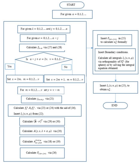
Figure 1. Algorithm for calculation of (LF) coefficients via (25).

Our next task is to apply the procedure to produce the first few (LF) scattering coefficients for a general impenetrable scatterer and then to apply the results for a spherical scatterer, in order to elucidate further its implementation. This task is realized in the next three sections.

4. Implementation for ${\mathit{u}}_{\mathit{0}}^{+}$

We start with Step 1 and apply (25) to acquire $u_0^{+}$ in the form

$$u_0^{+}\left(\mathbf{r}\right)=1+i^{-1}\sum _{\lambda =0}^{\infty }{r}^{-\lambda -1}{F}_{\lambda ,1}\left(\widehat{\mathbf{r}}\right)$$

(32)

where $F_{\lambda ,1}\left(\widehat{\mathbf{r}}\right)$ are given via (26) in the form

$$F_{\lambda ,1}\left(\widehat{\mathbf{r}}\right)=\sum _{\mu =-\lambda }^{\lambda }{f}_{\lambda ,\lambda }^{\mu }{A}_0^{\lambda ,\mu }{Y}_{\lambda }^{\mu }\left(\widehat{\mathbf{r}}\right).$$

(33)

With $f_{\lambda ,\lambda }^{\mu }$ given in (26) and (27), we proceed to calculate $A_0^{\lambda ,\mu }$, i.e., the coefficient of $k^{\lambda +1}$ in $g_{\lambda }^{\mu }$, for $\lambda \ge 0$. By means of (18)–(22) and (24), we arrive at

$$\begin{array}{cc}\hfill A_0^{\lambda ,\mu }& =A(0,0,\lambda ,\mu )\hfill \\ \hfill & ={\displaystyle \frac{1}{i^{\lambda -1}(2\lambda +1)!!}}\left[R^{\lambda +2}{\int }_{S^2}{\displaystyle \frac{\lambda }{R}}{Y}_{\lambda }^{\mu }\left(\widehat{\mathbf{r}}\right)ds\left(\widehat{\mathbf{r}}\right)+I_S(0,\lambda ,\mu )\right]\hfill \end{array}$$

(34)

Using the orthogonality property (15) of $Y_{\lambda }^{\mu }$ in (34) we arrive at

$$A_0^{\lambda ,\mu }={\displaystyle \frac{I_S(0,\lambda ,\mu )}{i^{\lambda -1}(2\lambda +1)!!}}$$

(35)

for $\lambda =0,1,2,\dots$ and $\mu =\lambda ,\dots ,\lambda$. Inserting in (33), we have

$$F_{\lambda ,1}\left(\widehat{\mathbf{r}}\right)=\sum _{\mu =-\lambda }^{\lambda }{f}_{\lambda ,\lambda }^{\mu }{\displaystyle \frac{I_S(0,\lambda ,\mu )}{i^{\lambda -1}(2\lambda +1)!!}}{Y}_{\lambda }^{\mu }\left(\widehat{\mathbf{r}}\right).$$

(36)

Finally, inserting in (32), we obtain

$$u_0^{+}\left(\mathbf{r}\right)=1+\sum _{\lambda =0}^{\infty }\sum _{\mu =-\lambda }^{\lambda }{\displaystyle \frac{f_{\lambda ,\lambda }}{i^{\lambda }(2\lambda +1)!!}}{\displaystyle \frac{I_S(0,\lambda ,\mu )}{r^{\lambda +1}}}{Y}_{\lambda }^{\mu }\left(\widehat{\mathbf{r}}\right),r>\delta ,$$

(37)

where

$$\begin{array}{c}\hfill I_S(0,\lambda ,\mu )={\int }_S{u}_0^{+}\left({\mathbf{r}}^{\prime }\right){\displaystyle \frac{\partial }{\partial n^{\prime }}}\left({\left(r^{\prime }\right)}^{\lambda }{Y}_{\lambda }^{{\mu }^{*}}\left({\widehat{\mathbf{r}}}^{\prime }\right)\right)ds\left({\mathbf{r}}^{\prime }\right)\\ \hfill -{\int }_S\left({\displaystyle \frac{\partial }{\partial n^{\prime }}}{u}_0^{+}\left({\mathbf{r}}^{\prime }\right)\right){\left(r^{\prime }\right)}^{\lambda }{Y}_{\lambda }^{{\mu }^{*}}\left({\widehat{\mathbf{r}}}^{\prime }\right)ds\left({\mathbf{r}}^{\prime }\right).\end{array}$$

(38)

Moving to Step 2, expression (37) is readily applied to a specific scatterer by inserting specific boundary conditions. We recall at this point that the series (37) converges absolutely and uniformly for $r>R=\delta +ϵ$ for every $ϵ>0$. Whenever there are no singularities, (37) can be extended by analytical continuation to reach the boundary S, becoming a regular linear Fredholm integral equation. This is the case for a spherical scatterer $S_{\alpha }$, and we take this chance to check the validity of (37).

• The soft spherical scatterer
  Applying (37) for $\mathbf{r}=\alpha \widehat{\mathbf{r}}$ and using the orthogonality property of $Y_n^m$ on $u_0^{+}\left(\alpha \widehat{\mathbf{r}}\right)=0$, we obtain

  $$\left\{\begin{array}{c}\hfill I_{S_{\alpha }}(0,0,0)=-\alpha \sqrt{4\pi }\\ \hfill I_{S_{\alpha }}(0,\lambda ,\mu )=0,\lambda \ge 1,\mu =-\lambda ,\dots ,\lambda \end{array}\right.$$

  (39)
  Therefore, (37) becomes

  $$u_0^{+}\left(\mathbf{r}\right)=1+f_{0,0}{\displaystyle \frac{I_{S_{\alpha }}(0,0,0)}{r}}{Y}_0^0\left(\widehat{\mathbf{r}}\right)=1-{\displaystyle \frac{\alpha }{r}},r\ge \alpha .$$

  (40)
• The hard and the resistive spherical scatterer
  Since for $a=0$ the Robin boundary condition (31) coincides with the Neumann condition, we refer to both of them together. Applying (37) for ${\partial }_r{u}_0^{+}\left(\alpha \widehat{\mathbf{r}}\right)=0$ and using the orthogonality property of $Y_n^m$, we arrive at

  $$I_{S_{\alpha }}(0,\lambda ,\mu )=0,\lambda =0,1,2,\dots$$

  (41)

  which leads immediately to the well-known result

  $$u_0^{+}\left(\mathbf{r}\right)=1,r\ge \alpha .$$

  (42)

Next, we will go through the algorithm once more for deriving $u_1^{+}$.

5. Implementation for ${\mathit{u}}_{\mathit{1}}^{+}$

Step 1 for $u_1^{+}$ gives

$$u_1^{+}\left(\mathbf{r}\right)=\widehat{\mathbf{k}}·\mathbf{r}+\sum _{\lambda =0}^{\infty }\left[-{\displaystyle \frac{1}{r^{\lambda +1}}}{F}_{\lambda ,2}-{\displaystyle \frac{i}{r^{\lambda }}}{F}_{\lambda ,1}\right].$$

(43)

Having already calculated $F_{\lambda ,1}$ in (36), we turn to $F_{\lambda ,2}\left(\widehat{\mathbf{r}}\right)$, which is provided in (26) by means of $A_0^{\lambda +1,\mu }$ and $A_1^{\lambda ,\mu }$ in the form

$$\begin{array}{cc}\hfill F_{\lambda ,2}\left(\widehat{\mathbf{r}}\right)& =\sum _{\sigma =0}^1\sum _{\mu =-(\lambda +\sigma )}^{\lambda +\sigma }{f}_{\lambda +\sigma ,\lambda }{A}_{1-\sigma }^{\lambda +\sigma ,\mu }{Y}_{\lambda +\sigma }^{\mu }\left(\widehat{\mathbf{r}}\right)\hfill \\ \hfill & =\sum _{\mu =-\lambda }^{\lambda }{f}_{\lambda ,\lambda }{A}_1^{\lambda ,\mu }{Y}_{\lambda }^{\mu }\left(\widehat{\mathbf{r}}\right)+\sum _{\mu =-(\lambda +1)}^{\lambda +1}{f}_{\lambda +1,\lambda }{A}_0^{\lambda +1,\mu }{Y}_{\lambda +1}^{\mu }\left(\widehat{\mathbf{r}}\right).\hfill \end{array}$$

(44)

With $A_0^{\lambda +1,\mu }$ provided via (35), we turn to $A_1^{\lambda ,\mu }$. In view of (18)–(24) we obtain

$$\begin{array}{cc}\hfill & A_1^{\lambda ,\mu }=A(0,1,\lambda ,\mu )={\displaystyle \frac{j_{\lambda ,0}}{i^{\lambda -2}}}{I}_S(1,\lambda ,\mu )\hfill \\ \hfill & +{\displaystyle \frac{j_{\lambda ,0}}{i^{\lambda -2}}}{R}^{\lambda +2}{\int }_{S^2}\left({\displaystyle \frac{\lambda }{R}}{f}_1^{+}\left(R\widehat{\mathbf{r}}\right)-{\partial }_r{f}_1^{+}\left(R\widehat{\mathbf{r}}\right)\right)Y_{\lambda }^{{\mu }^{*}}\left(\widehat{\mathbf{r}}\right)ds\left(\widehat{\mathbf{r}}\right)\hfill \\ \hfill & =\dots ={\displaystyle \frac{I_S(1,\lambda ,\mu )}{i^{\lambda -2}(2\lambda +1)!!}},\hfill \end{array}$$

(45)

where $f_1^{+}$ is calculated via (22) and (23) as

$$f_1^{+}\left(\mathbf{r}\right)=\widehat{\mathbf{k}}·\mathbf{r}+I_S(0,0,0)Y_0^0\left(\widehat{\mathbf{r}}\right).$$

(46)

Inserting (45) and (35) in (44) we obtain

$$\begin{array}{cc}\hfill F_{\lambda ,2}\left(\widehat{\mathbf{r}}\right)& =\sum _{\mu =-\lambda }^{\lambda }{\displaystyle \frac{f_{\lambda ,\lambda }}{i^{\lambda -2}(2\lambda +1)!!}}{I}_S(1,\lambda ,\mu )Y_{\lambda }^{\mu }\left(\widehat{\mathbf{r}}\right)\hfill \\ \hfill & +\sum _{\mu =-(\lambda +1)}^{\lambda +1}{\displaystyle \frac{f_{\lambda +1,\lambda }}{i^{\lambda }(2\lambda +3)!!}}{I}_S(0,\lambda +1,\mu )Y_{\lambda +1}^{\mu }\left(\widehat{\mathbf{r}}\right).\hfill \end{array}$$

(47)

Finally, inserting (36) and (47) in (43) we arrive at $u_1^{+}$ in the exterior of $S_{\delta }$

$$\begin{array}{cc}\hfill u_1^{+}\left(\mathbf{r}\right)=& \widehat{\mathbf{k}}·\mathbf{r}+\left(I_S(0,0,0)+{\displaystyle \frac{I_S(1,0,0)}{r}}\right)Y_0^0\left(\widehat{\mathbf{r}}\right)\hfill \\ \hfill & +\sum _{\lambda =1}^{\infty }\sum _{\mu =-\lambda }^{\lambda }{\displaystyle \frac{f_{\lambda ,\lambda }}{(2\lambda +1)!!i^{\lambda }}}{\displaystyle \frac{I_S(1,\lambda ,\mu )}{r^{\lambda +1}}}{Y}_{\lambda }^{\mu }\left(\widehat{\mathbf{r}}\right)\hfill \\ \hfill & +\sum _{\lambda =1}^{\infty }\sum _{\mu =-\lambda }^{\lambda }\left[{\displaystyle \frac{f_{\lambda ,\lambda }}{i^{\lambda }}}+{\displaystyle \frac{f_{\lambda ,\lambda -1}}{i^{\lambda +1}}}\right]{\displaystyle \frac{I_S(0,\lambda ,\mu )}{(2\lambda +1)!!r^{\lambda }}}{Y}_{\lambda }^{\mu }\left(\widehat{\mathbf{r}}\right).\hfill \end{array}$$

(48)

Expression (48) provides $u_1^{+}$ for any smooth impenetrable scatterer. With $I_S(0,\lambda ,\mu )$ already calculated in the course of $u_0^{+}$, for the specific boundary condition, we continue for the determination of the rest unknown integrals, and this is what we carry out for the spherical case.

• The Dirichlet problem
  Employing (48) for $u_1^{+}\left(\alpha \widehat{\mathbf{r}}\right)=0$ on $S=S_{\alpha }$ and using (30) to replace $\widehat{\mathbf{k}}·\mathbf{r}$ with the corresponding spherical harmonics, we have

  $$\begin{array}{cc}\hfill & u_1^{+}\left(\alpha \widehat{\mathbf{r}}\right)=\alpha \sqrt{{\displaystyle \frac{4\pi }{3}}}{Y}_1^0\left(\widehat{\mathbf{r}}\right)+\left[I_S(0,0,0)+{\displaystyle \frac{I_S(1,0,0)}{\alpha }}\right]Y_0^0\left(\widehat{\mathbf{r}}\right)\hfill \\ \hfill & +\sum _{\lambda =1}^{\infty }\sum _{\mu =-\lambda }^{\lambda }{\displaystyle \frac{f_{\lambda ,\lambda }}{(2\lambda +1)!!i^{\lambda }}}{\displaystyle \frac{I_S(1,\lambda ,\mu )}{{\alpha }^{\lambda +1}}}{Y}_{\lambda }^{\mu }\left(\widehat{\mathbf{r}}\right)=0.\hfill \end{array}$$

  (49)
  Using (39) and invoking orthogonality of $Y_{\lambda }^{\mu }$ on $S_{\alpha }$, we obtain

  $$\left\{\begin{array}{c}\hfill I_{S_{\alpha }}(1,0,0)=-\alpha I_{S_{\alpha }}(0,0,0)={\alpha }^2\sqrt{4\pi }\\ \hfill I_{S_{\alpha }}(1,1,0)=-3{\alpha }^3\sqrt{{\displaystyle \frac{4\pi }{3}}}\\ \hfill I_{S_{\alpha }}(1,1,\mu )=0,\mu =-1,1\\ \hfill I_{S_{\alpha }}(1,\lambda ,\mu )=0,\lambda \ge 2,\mu =-\lambda ,\dots ,\lambda \end{array}\right.$$

  (50)

  which leads straightforwardly to the well-known result [12]

  $$u_1^{+}\left(\mathbf{r}\right)=\widehat{\mathbf{k}}·\mathbf{r}-\alpha +{\displaystyle \frac{{\alpha }^2}{r}}-{\displaystyle \frac{{\alpha }^3}{r^2}}cos(\widehat{\mathbf{k}}·\widehat{\mathbf{r}}).$$

  (51)
• The Neumann problem
  Following similar arguments for the boundary condition ${\partial }_r{u}_1^{+}\left(\alpha \widehat{\mathbf{r}}\right)=0$ and using (48), (30), (41) and orthogonality of $Y_n^m$, we obtain

  $$\left\{\begin{array}{c}\hfill I_{S_{\alpha }}(1,0,0)=0\\ \hfill I_{S_{\alpha }}(1,1,0)={\displaystyle \frac{3{\alpha }^3}{2}}\sqrt{{\displaystyle \frac{4\pi }{3}}}\\ \hfill I_{S_{\alpha }}(1,1,\mu )=0\mu =-1,1\\ \hfill I_{S_{\alpha }}(1,\lambda ,\mu )=0\lambda \ge 2,\mu =-\lambda ,\dots ,\lambda \end{array}\right.$$

  (52)
  Substituting in (48) we arrive at the known result for the hard sphere

  $$u_1^{+}\left(\mathbf{r}\right)=\widehat{\mathbf{k}}·\mathbf{r}+{\displaystyle \frac{{\alpha }^3}{2r^2}}(\widehat{\mathbf{k}}·\widehat{\mathbf{r}}).$$

  (53)
• The Robin problem
  Employing (48) on the boundary condition ${\partial }_r{u}_1^{+}\left(\alpha \widehat{\mathbf{r}}\right)+\nu u_0^{+}\left(\alpha \widehat{\mathbf{r}}\right)=0$ and using (41) and (42) for the corresponding $u_0^{+}$ and also (30) for introducing $Y_n^m$, we arrive at

  $$\begin{array}{cc}\hfill & \sqrt{{\displaystyle \frac{4\pi }{3}}}{Y}_1^0\left(\widehat{\mathbf{r}}\right)-{\displaystyle \frac{I_S(1,0,0)}{{\alpha }^2}}{Y}_0^0\left(\widehat{\mathbf{r}}\right)\hfill \\ \hfill & +\sum _{\lambda =1}^{\infty }\sum _{\mu =-\lambda }^{\lambda }{\displaystyle \frac{(-\lambda -1)f_{\lambda ,\lambda }}{i^{\lambda }(2\lambda +1)!!}}{\displaystyle \frac{I_S(1,\lambda ,\mu )}{{\alpha }^{\lambda +2}}}{Y}_{\lambda }^{\mu }\left(\widehat{\mathbf{r}}\right)+\nu \sqrt{4\pi }{Y}_0^0\left(\widehat{\mathbf{r}}\right)=0.\hfill \end{array}$$

  (54)
  By exploiting orthogonality of $Y_{\lambda }^{\mu }$ on $S_{\alpha }$, we obtain

  $$\left\{\begin{array}{c}\hfill I_{S_{\alpha }}(1,0,0)=\nu {\alpha }^2\sqrt{4\pi }\\ \hfill I_{S_{\alpha }}(1,1,0)={\displaystyle \frac{-3{\alpha }^3}{2}}\sqrt{{\displaystyle \frac{4\pi }{3}}}\\ \hfill I_{S_{\alpha }}(1,1,\mu )=0\mu =-1,1\\ \hfill I_{S_{\alpha }}(1,\lambda ,\mu )=0\lambda \ge 2,\mu =-\lambda ,\dots ,\lambda .\end{array}\right.$$

  (55)
  Finally, (48) in view of (55) provides

  $$u_1^{+}\left(\mathbf{r}\right)=\widehat{\mathbf{k}}·\mathbf{r}+\nu {\displaystyle \frac{{\alpha }^2}{r}}+{\displaystyle \frac{{\alpha }^3}{2r^2}}(\widehat{\mathbf{k}}·\widehat{\mathbf{r}}),$$

  (56)

  which is the well-known result for the Robin result for the sphere [12].

In the next section, we will demonstrate only the highlights of the proposed algorithmic procedure to produce the next (LF) coefficient $u_2^{+}$ for the general smooth impenetrable scatterer. The basic arguments have already been presented in the previous sections, but the calculations, non surprisingly, become more complicated and cumbersome. Previous results enter in the process; therefore, one cannot escape calculating all lower order (LF) coefficients before proceeding to the next one.

6. Implementation for ${\mathit{u}}_{\mathit{2}}^{+}$

Beginning with Step 1, (25) for $a=2$, introduces $u_2^{+}$ in the form

$$\begin{array}{cc}\hfill u_2^{+}\left(\mathbf{r}\right)& ={\left(\widehat{\mathbf{k}}·\mathbf{r}\right)}^2+\sum _{\lambda =0}^{\infty }{\displaystyle \frac{2}{i^3{r}^{\lambda +1}}}{F}_{\lambda ,3}\left(\widehat{\mathbf{r}}\right)\hfill \\ \hfill & +\sum _{\lambda =0}^{\infty }\left[{\displaystyle \frac{2}{i^2{r}^{\lambda }}}{F}_{\lambda ,2}\left(\widehat{\mathbf{r}}\right)+{\displaystyle \frac{1}{i{r}^{1-\lambda }}}{F}_{\lambda ,1}\left(\widehat{\mathbf{r}}\right)\right].\hfill \end{array}$$

(57)

The new term to be calculated is $F_{\lambda ,3}\left(\widehat{\mathbf{r}}\right),$ which, in view of (26) is written as

$$\begin{array}{cc}\hfill F_{\lambda ,3}\left(\widehat{\mathbf{r}}\right)& =\sum _{\mu =-\lambda }^{\lambda }{f}_{\lambda ,\lambda }{A}_2^{\lambda ,\mu }{Y}_{\lambda }^{\mu }\left(\widehat{\mathbf{r}}\right)+\sum _{\mu =-(\lambda +1)}^{\lambda +1}{f}_{\lambda +1,\lambda }{A}_1^{\lambda +1,\mu }{Y}_{\lambda +1}^{\mu }\left(\widehat{\mathbf{r}}\right)\hfill \\ \hfill & +\sum _{\mu =-(\lambda +2)}^{\lambda +2}{f}_{\lambda +2,\lambda }{A}_0^{\lambda +2,\mu }{Y}_{\lambda +2}^{\mu }\left(\widehat{\mathbf{r}}\right).\hfill \end{array}$$

(58)

Now, utilizing (34) and (45) we turn to calculate $A_2^{\lambda ,\mu }$, via (18) in the form

$$A_2^{\lambda ,\mu }=\sum _{m=0}^{1}A(1-m,2m,\lambda ,\mu )=A(1,0,\lambda ,\mu )+A(0,2,\lambda ,\mu ).$$

(59)

After long but straightforward calculations to collect all necessary terms using (20)–(24) and (27)–(29) we end up at

$$\begin{array}{cc}\hfill & A(0,2,\lambda ,\mu )={\displaystyle \frac{1}{2i^{-3}}}\left(-2R^3{\displaystyle \frac{\sqrt{4\pi }}{3}}+I_S(0,0,0)\right){\delta }_{\lambda ,0}{\delta }_{\mu ,0}\hfill \\ \hfill & +{\displaystyle \frac{1}{(2\lambda +1)!!2i^{\lambda -3}}}[I_S(2,\lambda ,\mu )+I_S(0,\lambda ,\mu )(1-{\delta }_{\lambda ,0})].\hfill \end{array}$$

(60)

Inserting in (58) and then in (57), together with all previously calculated terms, we obtain $u_2^{+}$ for a general smooth impenetrable scatterer, in the form

$$\begin{array}{cc}\hfill & u_2^{+}\left(\mathbf{r}\right)={(\widehat{\mathbf{k}}·\mathbf{r})}^2+\left[(R^2+r^2+1){\displaystyle \frac{I_S(0,0,0)}{r}}+2I_S(1,0,0)+{\displaystyle \frac{I_S(2,0,0)}{r}}\right]Y_0^0\left(\widehat{\mathbf{r}}\right)\hfill \\ \hfill & +\sum _{\mu =-1}^1\left[\left({\displaystyle \frac{R^2}{3}}-r^2+1\right){\displaystyle \frac{I_S(0,1,\mu )}{3r^2}}+{\displaystyle \frac{I_S(2,1,\mu )}{3r^2}}\right]Y_1^{\mu }\left(\widehat{\mathbf{r}}\right)\hfill \\ \hfill & +\sum _{\lambda =2}^{\infty }\sum _{\mu =-\lambda }^{\lambda }\left[\left({\displaystyle \frac{R^2}{2\lambda +1}}+r^2+1\right){\displaystyle \frac{f_{\lambda ,\lambda }}{r^{\lambda +1}}}+{\displaystyle \frac{2f_{\lambda ,\lambda -1}}{i{r}^{\lambda -1}}}-{\displaystyle \frac{f_{\lambda ,\lambda -2}}{r^{\lambda -1}}}\right]{\displaystyle \frac{I_S(0,\lambda ,\mu )Y_{\lambda }^{\mu }\left(\widehat{\mathbf{r}}\right)}{i^{\lambda }(2\lambda +1)!!}}\hfill \\ \hfill & +\sum _{\lambda =2}^{\infty }\sum _{\mu =-\lambda }^{\lambda }\left[I_S(1,\lambda ,\mu )\left({\displaystyle \frac{2f_{\lambda ,\lambda }}{r^{\lambda }}}+{\displaystyle \frac{2f_{\lambda ,\lambda -1}}{i{r}^{\lambda }}}\right)+{\displaystyle \frac{I_S(2,\lambda ,\mu )f_{\lambda ,\lambda }}{r^{\lambda +1}}}\right]{\displaystyle \frac{Y_{\lambda }^{\mu }\left(\widehat{\mathbf{r}}\right)}{i^{\lambda }(2\lambda +1)!!}}.\hfill \end{array}$$

(61)

This formula is ready to be applied to specific boundary condition, in order to satisfy a specific scattering problem. Next, we will demonstrate only the implementation of (61) for a soft spherical scatterer $S_{\alpha }$, while the hard and resistive scatterer follows a similar track of arguments.

• The Dirichlet problem
  Applying (61) in the Dirichlet condition $u_2^{+}\left(\alpha \widehat{\mathbf{r}}\right)=0$ and using (39) and (50) along with (29), we have

  $$\begin{array}{cc}\hfill & u_2^{+}\left(\mathbf{r}\right)=\left({\displaystyle \frac{\sqrt{4\pi }}{3}}{Y}_0^0\left(\widehat{\mathbf{r}}\right)+{\displaystyle \frac{2}{3}}\sqrt{{\displaystyle \frac{4\pi }{5}}}{Y}_2^0\left(\widehat{\mathbf{r}}\right)\right){\alpha }^2\hfill \\ \hfill & +\left[-(2{\alpha }^2+1)\alpha \sqrt{4\pi }+2{\alpha }^2\sqrt{4\pi }+{\displaystyle \frac{I_S(2,0,0)}{a}}\right]Y_0^0\left(\widehat{\mathbf{r}}\right)\hfill \\ \hfill & +\sum _{\mu =-1}^1{\displaystyle \frac{I_S(2,1,\mu )}{3{\alpha }^2}}{Y}_1^{\mu }\left(\widehat{\mathbf{r}}\right)+\sum _{\lambda =2}^{\infty }\sum _{\mu =-\lambda }^{\lambda }{\displaystyle \frac{I_S(2,\lambda ,\mu )f_{\lambda ,\lambda }}{{\alpha }^{\lambda +1}}}{\displaystyle \frac{Y_{\lambda }^{\mu }\left(\widehat{\mathbf{r}}\right)}{i^{\lambda }(2\lambda +1)!!}}=0.\hfill \end{array}$$

  (62)
  Invoking orthogonality of $Y_n^m$ on $S_{\alpha }$, we obtain

  $$\left\{\begin{array}{c}\hfill I_{S_{\alpha }}(2,0,0)=\alpha \sqrt{4\pi }(1-{\displaystyle \frac{{\alpha }^2}{3}})\\ \hfill I_{S_{\alpha }}(2,1,\mu )=0,\mu =-1,0,1\\ \hfill I_{S_{\alpha }}(2,2,0)=-{\displaystyle \frac{10}{3}}\sqrt{{\displaystyle \frac{4\pi }{5}}}{\alpha }^5\\ \hfill I_{S_{\alpha }}(2,2,\mu )=0,\mu =-2,-1,1,2\\ \hfill I_{S_{\alpha }}(2,\lambda ,\mu )=0,\lambda \ge 2,\mu =-\lambda ,\dots ,\lambda .\end{array}\right.$$

  (63)
  Substituting (63) in (62) and elaborating further on the result, with the aid of (29) and (17), we arrive at the well-known formula [12]

  $$\begin{array}{cc}\hfill u_2^{+}\left(\mathbf{r}\right)=& {\displaystyle \frac{2}{3}}{P}_2^0(\widehat{\mathbf{k}}·\widehat{\mathbf{r}})(r^2-{\displaystyle \frac{{\alpha }^5}{r^3}})+{\displaystyle \frac{r^2}{3}}-{\displaystyle \frac{4{\alpha }^3}{3r}}-\alpha r+2{\alpha }^2.\hfill \end{array}$$

  (64)

7. Discussion

In the present paper, a new algorithm is developed for the calculation of the Low Frequency expansion of the total acoustic field scattered by a convex object of arbitrary shape with a $C^2$ smooth impenetrable boundary that has been excited by a plane incident wave.

The algorithm includes mainly algebraic operators, accelerating greatly the calculation of any order low frequency approximation of the total wave field satisfying a specific scattering problem, where the scatterer is considered bounded by a smooth, at least $C^2$, convex, impenetrable surface S. An integral operator is included in the last step of the algorithm, that still, due to the separateness and regularity of its integral kernel, is safely handled analytically or numerically, with respect to the scatterer boundary.

In particular, by exploiting analyticity of the scattering amplitude g in low frequencies and in all directions, and also the smoothness of the scatterer’ s boundary, in view of the Atkinson—Wilcox theorem, an integral representation of every low frequency coefficient $u_a^{+}$ is provided, in the exterior of the scatterer’ s circumscribing sphere. The integral kernel is continuous and separable including a surface spherical harmonic of some degree. The representation becomes an integral equation on S, if surface S is reachable by analytical continuation. If this is not the case, our method offers the advantage of minimizing the discretization space for applying any numerical scheme, to the limited space between S and its circumscribing sphere. Therefore, a bounded and continuous mapping is produced both between the spherical coefficients of g or the low frequency scattering coefficients $u_a^{+}$ and the boundary values of the coefficients $u_n^{+},n\le a$, enabling efficient and reliable numerical computation of any low frequency approximation. Thus, the proposed algorithm can be especially useful in inverse scattering problems while any order of scattering approximations can be calculated in a stable, fast, and reliable fashion.

Moreover, the paper provides ready to be applied formulae for the first coefficients $u_0^{+},u_1^{+},u_2^{+}$, as well as the algorithmic procedure to produce any finite low frequency approximation in a clear encoded fashion, for any smooth impenetrable scatterer. The formulae are checked to recover known results for a spherical scatterer, yielding the validity of the proposed procedure.

8. Conclusions

The time suppressed solution of the direct acoustic scattering problem in the low frequency regime is provided for arbitrarily shaped convex scatterers with smooth impenetrable boundary, in view of plane wave excitation. The scattering coefficients are provided in the form of power series of inverse powers of the distance, where the coefficients are calculated by means of a clearly presented, stable algorithm, including algebraic and linear regular integral operators.

The methodology approach is based on the far field expansion of the total wave, which is uniformly convergent in the exterior of the scatterer’ s circumscribing sphere, combined with its low frequency expansion in the space between. Theoretically justified, the fruit of this combination is Formula (25), by which the Low Frequency approximation of order a, of the total acoustic field, $u_a^{+}$, is calculated for $a=0,1,2,\dots$, namely

$$u_a^{+}\left(\mathbf{r}\right)={(\widehat{\mathbf{k}}·\mathbf{r})}^a+\sum _{\lambda =0}^{\infty }\sum _{j=0}^a{\displaystyle \frac{a!}{j!}}{i}^{j-a-1}{r}^{j-\lambda -1}{F}_{\lambda ,a-j+1}\left(\widehat{\mathbf{r}}\right),$$

(65)

where all the parameters and functions involved have been introduced in Section 3. The formula holds outside of the scatterer’ s circumscribing sphere, for any convex scatterer with an impenetrable boundary, sufficiently smooth ($C^2$) in order for the Gauss–Green theorems to apply. The corresponding boundary is introduced in function F via surface integrals of the form

$$\begin{array}{c}\hfill I_S(x,n,\mu )={\int }_S{u}_x^{+}\left({\mathbf{r}}^{\prime }\right){\displaystyle \frac{\partial }{\partial n^{\prime }}}\left[{\left(r^{\prime }\right)}^n{Y}_n^{{\mu }^{*}}\left({\widehat{\mathbf{r}}}^{\prime }\right)\right]ds\left({\widehat{\mathbf{r}}}^{\prime }\right)\\ \hfill -{\int }_S\left[{\displaystyle \frac{\partial }{\partial n^{\prime }}}{u}_x^{+}\left({\mathbf{r}}^{\prime }\right)\right]{\left(r^{\prime }\right)}^n{Y}_n^{{\mu }^{*}}\left({\widehat{\mathbf{r}}}^{\prime }\right)ds\left({\widehat{\mathbf{r}}}^{\prime }\right),\end{array}$$

(66)

for $x=0,1,\dots ,a$. Additionally, the paper provides the explicit formulae (37), (48) and (61) for the first three coefficients, in order to demonstrate the implementation of (25) via the proposed procedure. These expressions are, to our knowledge, novel providing directly the corresponding coefficients for such a wide class of scatterers.

These expressions are readily applied to any specific scatterer in the examined class, by inserting the corresponding boundary conditions. Nevertheless, each formula involves integrals of the form $I_S(a,y,\lambda ,\mu )$, which is dependent on the unknown coefficient $u_a^{+}$. Since the series converge absolutely and uniformly in the exterior of the scatterer’s circumscribing sphere, the direct employment of the boundary conditions is not straightforward. Whenever analytical continuation is feasible up to the boundary S, the corresponding boundary conditions are properly introduced, and each formula provides a regular linear Fredholm integral equation, easily handled to calculate the unknown integrals $I_S(a,y,\lambda ,\mu )$. The calculation of $u_a^{+}$ is then readily accomplished by introducing $I_S(a,y,\lambda ,\mu )$ in the corresponding formula. On the other hand, if analytical continuation is not possible, Formulae (25), (37), (48) and (61) provide $u_a^{+}$ by means of numerical calculation in the space between the scatterer’ s surface and its circumscribing sphere. Reducing the discretization space to such a restricted one offers an obvious advantage in terms of computational time and resources. Robust proofs of the construction of the algorithm are included in the following Appendix A, which can be intuitive for developing similar algorithms in other Scattering settings or physics, as in Electromagnetics or in elasticity. The implementation of the proposed procedure to provide new analytical results for special scatterers, as for example the spheroid or ellipsoid one, is in our immediate scopes.

Appendix A.1. Proof of Theorem 1

First, we prove Lemmas A1 and A2.

Lemma A1.

The scattering amplitude g of the problem (1), (2) with a boundary condition of the form (12), in the realm of the low frequencies, assumes the following expansion:

$$g(\widehat{\mathbf{r}};k)=\sum _{n=0}^{\infty }\sum _{\mu =-n}^n\sum _{\nu =n+1}^{\infty }{g}_{n,\nu }^{\mu }{k}^{\nu }{Y}_n^{\mu }\left(\widehat{\mathbf{r}}\right)$$

(A1)

Proof of Lemma A1.

Since the scattering amplitude g is an analytical function in $\widehat{\mathbf{r}}\in S^2$ and also in k, in the Rayleigh region, it assumes both a spherical expansion and, for $k\delta \ll 1$, an expansion of its spherical coefficients in powers of k, of the form (13). We will prove that $g_n^{\mu }\left(k\right)$ involves powers of k greater or equal to $n+1$, i.e., $\nu \ge n+1$. Using the orthogonality property of $Y_n^{\mu }$ in $S^2$, in the first equation of (13), we have

$$g_n^{\mu }\left(k\right)={\oint }_{S^2}g({\widehat{\mathbf{r}}}_1;k)Y_n^{{\mu }^{*}}\left({\widehat{\mathbf{r}}}_1\right)ds\left({\widehat{\mathbf{r}}}_1\right).$$

(A2)

We consider a spherical surface $S_R$, with $R=\delta +ϵ$ for $ϵ>0$, which includes S, and we insert the integral representation (4) on $S_R$, in (A2) to obtain

$$g_n^{\mu }\left(k\right)=-\frac{ik}{4\pi }{I}_1(k,n,\mu )-\frac{{\left(ik\right)}^2}{4\pi }{I}_2(k,n,\mu )$$

(A3)

where

$$I_1(k,n,\mu )={\int }_{S_R}{\partial }_{n_2}{u}^{+}\left({\mathbf{r}}_2\right)\left[{\oint }_{S^2}{e}^{-ik{\widehat{\mathbf{r}}}_1·{\mathbf{r}}_2}{Y}_n^{{\mu }^{*}}\left({\widehat{\mathbf{r}}}_1\right)ds\left({\widehat{\mathbf{r}}}_1\right)\right]ds\left({\widehat{\mathbf{r}}}_2\right)$$

(A4)

and

$$I_2(k,n,\mu )={\int }_{S_R}{u}^{+}\left({\mathbf{r}}_2\right){\widehat{\mathbf{n}}}_2·\left[{\oint }_{S^2}{e}^{-ik{\widehat{\mathbf{r}}}_1·{\mathbf{r}}_2}{\widehat{\mathbf{r}}}_1{Y}_n^{{\mu }^{*}}\left({\widehat{\mathbf{r}}}_1\right)ds\left({\widehat{\mathbf{r}}}_1\right)\right]ds\left({\widehat{\mathbf{r}}}_2\right).$$

(A5)

Next, we use in (A4) the complex conjugate of the Funk–Hecke formula [3]

$${\oint }_{S^2}{e}^{ik{\widehat{\mathbf{r}}}_1·{\mathbf{r}}_2}{Y}_n^{\mu }\left({\widehat{\mathbf{r}}}_1\right)ds\left({\widehat{\mathbf{r}}}_1\right)={\displaystyle \frac{4\pi }{{(-i)}^n}}{j}_n\left(k{r}_2\right)Y_n^{\mu }\left({\widehat{\mathbf{r}}}_2\right)$$

(A6)

and in (A5) the complex conjugate of the formula [30]

$${\oint }_{S^2}{e}^{ik{\widehat{\mathbf{r}}}_1·{\mathbf{r}}_2}{\widehat{\mathbf{r}}}_1{Y}_n^{\mu }\left({\widehat{\mathbf{r}}}_1\right)ds\left({\widehat{\mathbf{r}}}_1\right)=4\pi i^{n-1}\left[j_n^{\prime }\left(k{r}_2\right){\widehat{\mathbf{r}}}_2{Y}_n^{\mu }\left({\widehat{\mathbf{r}}}_2\right)+{\displaystyle \frac{j_n\left(k{r}_2\right)}{k{r}_2}}{\mathbf{D}}_a{Y}_n^{\mu }\left({\mathbf{r}}_2\right)\right]$$

(A7)

where $j_n$ is the spherical Bessel function of the $n^{th}$ degree; the prime denotes differentiation with respect to the argument and the operator ${\mathbf{D}}_a$ is defined as

$${\mathbf{D}}_a:=\widehat{\theta }{\displaystyle \frac{\partial }{\partial \theta }}+\widehat{\varphi }{\displaystyle \frac{1}{sin\theta }}{\displaystyle \frac{\partial }{\partial \varphi }}.$$

Inserting properly (A6) and (A7) in (A4) and (A5) respectively, together with the power series expansion of $j_n$ [31],

$$j_n\left(z\right)=\sum _{y=0}^{\infty }{j}_{n,y}{z}^{n+2y}$$

(A8)

where $j_{n,y}$ is given in (21) and also, exploiting the spherical symmetry which implies that ${\widehat{\mathbf{n}}}_2={\widehat{\mathbf{r}}}_2$, we obtain

$$I_1(k,n,\mu )={\displaystyle \frac{4\pi }{i^n}}\sum _{y=0}^{\infty }\left[{\int }_{S_R}{\partial }_{r_2}{u}^{+}\left({\mathbf{r}}_2\right)r_2^{n+2y}{Y}_n^{{\mu }^{*}}\left({\widehat{\mathbf{r}}}_2\right)ds\left({\mathbf{r}}_2\right)\right]j_{n,y}{k}^{n+2y}$$

(A9)

and

$$\begin{array}{c}\hfill I_2(k,n,\mu )={\displaystyle \frac{4\pi }{i^{n-1}}}\sum _{y=0}^{\infty }\left[{\int }_{S_R}{u}^{+}\left({\mathbf{r}}_2\right)(n+2y)r_2^{n+2y-1}{Y}_n^{{\mu }^{*}}\left({\widehat{\mathbf{r}}}_2\right)ds\left({\mathbf{r}}_2\right)\right]j_{n,y}{k}^{n+2y-1}.\end{array}$$

(A10)

Substituting (A9) and (A10) in (A3) and bearing in mind that $u^{+}$ is an analytical function in k, it is clear that $g_n^{\mu }$ involves powers of k greater or equal to $n+1$, namely

$$g_n^{\mu }\left(k\right)=\sum _{y=0}^{\infty }{I}_3(k,n,\mu ,y)k^{n+1+2y}$$

(A11)

where

$$\begin{array}{c}\hfill I_3(k,n,\mu ,y)={\displaystyle \frac{j_{n,y}{R}^{n+2y+2}}{i^{n-1}}}{\int }_{S^2}\left[{\displaystyle \frac{n+2y}{R}}{u}^{+}\left(R{\widehat{\mathbf{r}}}_2\right)-{\partial }_{r_2}{u}^{+}\left(R{\widehat{\mathbf{r}}}_2\right)\right]Y_n^{{\mu }^{*}}\left({\widehat{\mathbf{r}}}_2\right)ds\left({\widehat{\mathbf{r}}}_2\right).\end{array}$$

(A12)

□

Lemma A2.

Considering the problem at hand, the following equations hold true:

$$\begin{array}{cc}\hfill {\int }_{S^2}{u}_x^{+}\left(R\widehat{\mathbf{r}}\right)Y_n^{{\mu }^{*}}\left(\widehat{\mathbf{r}}\right)ds\left(\widehat{\mathbf{r}}\right)=& {\int }_{S^2}{f}_x^{+}\left(R\widehat{\mathbf{r}})\right)Y_n^{{\mu }^{*}}\left(\widehat{\mathbf{r}}\right)ds\left(\widehat{\mathbf{r}}\right)\hfill \\ \hfill & -{\displaystyle \frac{1}{2n+1}}{R}^{-n-1}{I}_S(x,n,\mu )\hfill \end{array}$$

(A13)

and

$$\begin{array}{cc}\hfill {\int }_{S^2}{\partial }_r{u}_x^{+}\left(R\widehat{\mathbf{r}}\right)Y_n^{{\mu }^{*}}\left(\widehat{\mathbf{r}}\right)ds\left(\widehat{\mathbf{r}}\right)=& {\int }_{S^2}{\partial }_r{f}_x^{+}\left(R\widehat{\mathbf{r}})\right)Y_n^{{\mu }^{*}}\left(\widehat{\mathbf{r}}\right)ds\left(\widehat{\mathbf{r}}\right)\hfill \\ \hfill & -{\displaystyle \frac{(n+1)}{(2n+1)}}{R}^{-n-2}{I}_S(x,n,\mu )\hfill \end{array}$$

(A14)

where $R=\delta +ϵ$ with $ϵ>0$, $I_S(x,n,\mu )$ is the scatterer’ s boundary integral defined in (22) and $f_x^{+}\left(R\widehat{\mathbf{r}})\right)$ given in (23), (24).

Proof of Lemma A2.

We recall the integral representation of $u_x^{+}$, Ref. [12] for $\mathbf{r}=R\widehat{\mathbf{r}}$, namely

$$\begin{array}{c}\hfill u_x^{+}\left(R\widehat{\mathbf{r}}\right)=f_x^{+}\left(R\widehat{\mathbf{r}}\right)+{\displaystyle \frac{1}{4\pi }}{\int }_S\left[u_x^{+}\left({\mathbf{r}}^{\prime }\right){\displaystyle \frac{\partial }{\partial n^{\prime }}}{\displaystyle \frac{1}{|\mathbf{r}-{\mathbf{r}}^{\prime }|}}-{\displaystyle \frac{1}{|\mathbf{r}-{\mathbf{r}}^{\prime }|}}{\displaystyle \frac{\partial }{\partial n^{\prime }}}{u}_x^{+}\left({\mathbf{r}}^{\prime }\right)\right]ds\left({\mathbf{r}}^{\prime }\right)\end{array}$$

(A15)

where $f_x^{+}$ is given in (23) and (24), and we insert the spherical expansion (16) of ${\displaystyle \frac{1}{\left|\mathbf{r}-{\mathbf{r}}^{\prime }\right|}}$, for $r=R=\delta +ϵ>r^{\prime }$, since ${\mathbf{r}}^{\prime }\in S$. Using orthogonality of $Y_n^{\mu }$, we end up at (A13) and (A14) in a straightforward manner. □

We turn now to prove Theorem 1. Regarding this, we need to rewrite (A11) as a power series of k, which first implies the task to extract the powers of k hidden in $u^{+}$ and ${\partial }_{n_2}{u}^{+}$ in the integrands of (A12). We begin the proof with that task.

Proof of Theorem 1 .

We insert the low frequency expansions of $u^{+}$ and ${\partial }_{n_2}{u}^{+}$ from (7) in the integrands of (A11) and apply the Cauchy product formula. After appropriate elaboration of the series, we end up at the following:

$$g_n^{\mu }\left(k\right)=k^{n+1}\sum _{p=0}^{\infty }\sum _{N=p}^{2p}{k}^N{\displaystyle \frac{j_{n,N-p}}{(2p-N)!i^{n-1-(2p-N)}}}{J}_{S_R}(N-p,2p-N,n,\mu )$$

(A16)

where

$$\begin{array}{cc}\hfill & J_{S_R}(N-p,2p-N,n,\mu )=R^{n+2(N-p)+2}\times \hfill \\ \hfill & \times {\int }_{S^2}\left[{\displaystyle \frac{n+2(N-p)}{R}}{u}_{2p-N}^{+}\left(R\widehat{\mathbf{r}}\right)-{\partial }_n{u}_{2p-N}^{+}\left(R\widehat{\mathbf{r}}\right)\right]Y_n^{{\mu }^{*}}\left(\widehat{\mathbf{r}}\right)ds\left(\widehat{\mathbf{r}}\right).\hfill \end{array}$$

(A17)

By opening up the series and rearranging properly the terms, (A16) is written as

$$g_n^{\mu }\left(k\right)=k^{n+1}{A}_0^{n,\mu }+\sum _{N=n+2}^{\infty }{k}^N{A}_{N-n-1}^{n,\mu }$$

(A18)

where $A_{N-n-1}^{n,\mu }$ is defined with respect to the parity of the parameter $N-n-1$, as in (18) and (19) with

$$A(y,x,n,\mu )={\displaystyle \frac{j_{n,y}}{x!i^{n-1-x}}}{J}_{S_R}(y,x,n,\mu )$$

(A19)

and $J_{S_R}(y,x,n,\mu )$ as in (A17) with $x=2p-N=0,1,2,\dots ,p$ and $y=N-p\ge 0$, namely

$$\begin{array}{c}\hfill J_{S_R}(y,x,n,\mu )=R^{n+2y+2}{\int }_{S^2}\left[{\displaystyle \frac{n+2y}{R}}{u}_x^{+}\left(R\widehat{\mathbf{r}}\right)-{\partial }_n{u}_x^{+}\left(R\widehat{\mathbf{r}}\right)\right]Y_n^{{\mu }^{*}}\left(\widehat{\mathbf{r}}\right)ds\left(\widehat{\mathbf{r}}\right).\end{array}$$

(A20)

Our final task is to prove that these integrals are actually those defined in (20)–(22). This is readily accomplished by inserting (A13) and (A14) in (A20), which completes the proof of Theorem 1.

Appendix A.2. Proof of Theorem 2

Proof of Theorem 2.

First, we invoke the far field expansion (9) and the (AW) coefficients, which, calculated from the recurrence relation (10) by means of (11), provide

$$\begin{array}{cc}\hfill F_m\left(\widehat{\mathbf{r}}\right)& ={\displaystyle \frac{1}{{\left(2ik\right)}^{2}m(m-1)}}[\mathbb{B}+m(m-1)][\mathbb{B}+(m-1)(m-2)]F_{m-2}\left(\widehat{\mathbf{r}}\right)\hfill \\ \hfill & =\dots ={\displaystyle \frac{1}{{\left(2ik\right)}^{m}m!}}\{\prod _{j=1}^m[\mathbb{B}+(m-j+1)(m-j)]\}g\left(\widehat{\mathbf{r}}\right).\hfill \end{array}$$

(A21)

Now, we insert (13) and recall that $\left(Y_n^m,-n(n+1)\right)$ is an eigenpair of the Beltrami operator. Hence, the coefficients $F_m$, for $m\ge 1$ can be written as

$$\begin{array}{c}\hfill F_m\left(\widehat{\mathbf{r}}\right)=\sum _{n=m}^{\infty }\sum _{\mu =-n}^n{\displaystyle \frac{{\prod }_{j=1}^m[-n(n+1)+(m-j+1)(m-j)]}{{\left(2ik\right)}^{m}m!}}{g}_n^{\mu }\left(k\right)Y_n^{\mu }\left(\widehat{\mathbf{r}}\right)\end{array}$$

(A22)

while, due to (17), we deduce

$$\begin{array}{c}\hfill F_m\left(\widehat{\mathbf{r}}\right)=\sum _{n=m}^{\infty }\sum _{\mu =-n}^n\sum _{\nu =n+1-m}^{\infty }{f}_{n,m}{A}_{\nu +m-n-1}^{n,\mu }{Y}_n^{\mu }\left(\widehat{\mathbf{r}}\right)k^{\nu }\end{array}$$

(A23)

where

$$f_{n,m}={\displaystyle \frac{1}{{\left(2i\right)}^{m}m!}}\{\prod _{j=1}^m[-n(n+1)+(m-j+1)(m-j)]\}.$$

(A24)

The terms for $n<m$ vanish, since the product in these terms always includes a zero coefficient. Expression (A23) holds also for $m=0$, if, in view of (11) we define $f_{n,0}=1$.

Opening up the series and rearranging the terms in increasing powers of k, (A23) can be written, for $m=0,1,2,\dots$ as

$$\begin{array}{cc}\hfill F_m\left(\widehat{\mathbf{r}}\right)& =k^1{A}_0^m{f}_{m,m}\sum _{\mu =-m}^m{Y}_m^{\mu }\left(\widehat{\mathbf{r}}\right)\hfill \\ \hfill & +k^2[A_1^m{f}_{m,m}\sum _{\mu =-m}^m{Y}_m^{\mu }\left(\widehat{\mathbf{r}}\right)+A_0^{m+1}{f}_{m+1,m}\sum _{\mu =-m-1}^{m+1}{Y}_{m+1}^{\mu }\left(\widehat{\mathbf{r}}\right)]\hfill \\ \hfill & +k^3[A_2^m{f}_{m,m}\sum _{\mu =-m}^m{Y}_m^{\mu }\left(\widehat{\mathbf{r}}\right)+A_1^{m+1}{f}_{m+1,m}\sum _{\mu =-m-1}^{m+1}{Y}_{m+1}^{\mu }\left(\widehat{\mathbf{r}}\right)\hfill \\ \hfill & +A_0^{m+2}{f}_{m+2,m}\sum _{\mu =-m-2}^{m+2}{Y}_{m+2}^{\mu }\left(\widehat{\mathbf{r}}\right)]+\dots =\sum _{\nu =1}^{\infty }{F}_{m,\nu }\left(\widehat{\mathbf{r}}\right)k^{\nu }\hfill \end{array}$$

(A25)

with

$$F_{m,\nu }\left(\widehat{\mathbf{r}}\right)=\sum _{\sigma =0}^{\nu -1}\sum _{\mu =-(m+\sigma )}^{m+\sigma }{f}_{m+\sigma ,m}{A}_{\nu -\sigma -1}^{m+\sigma ,\mu }{Y}_{m+\sigma }^{\mu }\left(\widehat{\mathbf{r}}\right).$$

(A26)

We turn now to the expansion (9), which, using the power series expansion of the exponential and applying the Cauchy product formula, we obtain for $r>\delta$

$$\begin{array}{cc}\hfill u\left(\mathbf{r}\right)& ={\displaystyle \frac{e^{ikr}}{ikr}}\sum _{m=0}^{\infty }{\displaystyle \frac{F_m\left(\widehat{\mathbf{r}}\right)}{r^m}}=\sum _{j=0}^{\infty }\sum _{m=0}^j\frac{{\left(ik\right)}^{j-m-1}}{(j-m)!}{F}_m\left(\widehat{\mathbf{r}}\right)r^{j-2m-1}.\hfill \end{array}$$

(A27)

Inserting (A25), rearranging the terms in increasing powers of k and, carrying out cumbersome calculations, we obtain

$$\begin{array}{c}\hfill u\left(\mathbf{r}\right)=\sum _{a=0}^{\infty }{\displaystyle \frac{{\left(ik\right)}^a}{a!}}\sum _{\lambda =0}^{\infty }\sum _{j=0}^a{\displaystyle \frac{a!}{j!}}{i}^{j-a-1}{r}^{j-\lambda -1}{F}_{\lambda ,a-j+1}\left(\widehat{\mathbf{r}}\right).\end{array}$$

(A28)

Therefore, the (LF) coefficients of the problem, for $a=0,1,2,\dots$, are

$$\begin{array}{c}\hfill u_a^{+}\left(\mathbf{r}\right)={(\widehat{\mathbf{k}}·\mathbf{r})}^a+\sum _{\lambda =0}^{\infty }\sum _{j=0}^a{\displaystyle \frac{a!}{j!}}{i}^{j-a-1}{r}^{j-\lambda -1}{F}_{\lambda ,a-j+1}\left(\widehat{\mathbf{r}}\right)\end{array}$$

(A29)

and Theorem 2 has been proved. □

References

- Colton, D.; Kress, R. Inverse Acoustic and Electromagnetic Scattering Theory; Springer: New York, NY, USA, 1998. [Google Scholar]
- Hadjinicolaou, M. Non-Destructive Identification of Spherical Inclusions. Adv. Compos. Lett. 2000, 9, 25–33. [Google Scholar] [CrossRef]
- Martin, P.A. Multiple Scattering. Interaction of Time Harmonic Waves with N Obstacles; Cambridge University Press: Cambridge, UK, 2006. [Google Scholar]
- Steinbach, O.; Unger, G. Combined boundary integral equations for acoustic scattering resonance problems. Math. Methods Appl. Sci. 2017, 40, 1516–1530. [Google Scholar] [CrossRef]
- Ar, E.; Kleinman, R.E. The exterior Neumann problem for the three dimensional Helmholtz equation. Arch. Ration. Mech. Anal. 1996, 23, 218–236. [Google Scholar] [CrossRef]
- Ammari, H.; Kang, H. Boundary layer techniques for solving the Helmholtz equation in the presence of small inhomogeneities. J. Math. Anal. Appl. 2004, 296, 190–208. [Google Scholar] [CrossRef]
- Charalambopoulos, A.; Gergidis, L.; Vassilopoulou, E. A Conditioned Probabilistic Method for the Solution of the Inverse Acoustic Scattering Problem. Mathematics 2022, 10, 1383. [Google Scholar] [CrossRef]
- Amirkulova, F.; Gerges, S.; Norris, A. Sound Localization through Multi-Scattering and Gradi-ent-Based Optimization. Mathematics 2021, 9, 2862. [Google Scholar] [CrossRef]
- Bellis, C.; Bonnet, M.; Cakoni, F. Acoustic inverse scattering using topological derivative of far-field measurements-based L-2 cost functionals. Inverse Probl. 2013, 29, 75012. [Google Scholar] [CrossRef]
- Zhang, D.; Guo, Y. Uniqueness results on phaseless inverse acoustic scattering with a reference ball. Inverse Probl. 2018, 34, 85002. [Google Scholar] [CrossRef]
- Donoso, L.; Feuillade, C. Geometrical modeling and analysis of low frequency acoustical scattering from cylindrically formed schools of swim bladder fish. J. Acoust. Soc. Am. 2020, 148, 2482. [Google Scholar] [CrossRef]
- Dassios, G.; Kleinman, R.E. Low Frequency Scattering; Oxford University Press: Oxford, UK, 2000. [Google Scholar]
- Colton, D.; Kress, R. Integral Equation Methods in Scattering Theory; Wiley-Interscience: New York, NY, USA, 1983. [Google Scholar]
- Martin, P.A. On the far-field computation of acoustic radiation forces. J. Acoust. Soc. Am. 2017, 142, 2094–2100. [Google Scholar] [CrossRef]
- Mahariq, I.; Giden, I.H.; Alboon, S.; Aly, W.H.F.; Youssef, A.; Kurt, H. Investigation and Analysis of Acoustojets by Spectral Element Method. Mathematics 2022, 10, 3145. [Google Scholar] [CrossRef]
- Kariotou, F.; Sinikis, D.E. An algebraic calculation method for the acoustic low frequency expansion. J. Math. Anal. Appl. 2015, 424, 1506–1529. [Google Scholar] [CrossRef]
- Kariotou, F.; Sinikis, D.E. An algebraic formula for the accelerated computation of the low frequency scattering coefficients: The case of the acoustically soft sphere. Appl. Math. Comput. 2016, 275, 13–23. [Google Scholar] [CrossRef]
- Kariotou, F.; Sinikis, D.E. An accelerated derivation of the acoustic low frequency expansion: The penetrable sphere. Math. Methods Appl. Sci. 2018, 41, 973–978. [Google Scholar] [CrossRef]
- Sommerfeld, A. Partial Differential Equations in Physics; Academic Press: New York, NY, USA, 1949. [Google Scholar]
- Atkinson, F.V. On Sommerfeld’s radiation condition. Philos. Mag. 1949, 40, 645–651. [Google Scholar] [CrossRef]
- Wilcox, C.H. A generalization of theorems of Rellich and Atkinson. Proc. Am. Math. Soc. 1965, 7, 271–276. [Google Scholar] [CrossRef]
- Kleinman, R.E. The Dirichlet problem for the Helmholtz equation. Arch. Ration. Mech. Anal. 1965, 18, 205–229. [Google Scholar] [CrossRef]
- Ammari, H.; Nedelec, J.-C. Full low-frequency asymptotics for the reduced wave equation. Appl. Math. Lett. 1999, 12, 127–131. [Google Scholar] [CrossRef]
- Tsitsas, N.; Athanasiadis, C. Point Source Excitation Of A Layered Sphere: Direct And Far-Field Inverse Scattering Problems. Q. J. Mech. Appl. Math. 2008, 61, 549–580. [Google Scholar] [CrossRef][Green Version]
- Dassios, G. The Atkinson–Wilcox theorem in ellipsoidal geometry. J. Math. Anal. Appl. 2002, 274, 828–845. [Google Scholar] [CrossRef][Green Version]
- Athanasiadis, C.; Giotopoulos, S. The Atkinson-Wilcox expansion theorem for electromagnetic chiral waves. Appl. Math. Lett. 2003, 16, 675–681. [Google Scholar] [CrossRef][Green Version]
- Dassios, G. The Atkinson–Wilcox expansion theorem for elastic waves. Q. Appl. Math. 1988, 46, 285–299. [Google Scholar] [CrossRef]
- Morse, P.M.; Feshbach, H. Methods of Theoretical Physics; McGraw Hill Co., Inc.: New York, NY, USA, 1953. [Google Scholar]
- Charalambopoulos, A.; Dassios, G. Inverse scattering via low-frequency moments. J. Math. Phys. 1992, 33, 4201–4216. [Google Scholar] [CrossRef]
- Dassios, G.; Rigou, Z. Elastic Herglotz functions. SIAM J. Appl. Math. 1995, 55, 1345–1361. [Google Scholar] [CrossRef]
- Abramowitz, M.; Stegun, I. Handbook of Mathematical Functions with Formulas, Graphs, and Mathematical Tables; Dover Publications: New York, NY, USA, 1964. [Google Scholar]
Publisher’s Note: MDPI stays neutral with regard to jurisdictional claims in published maps and institutional affiliations. |
© 2022 by the authors. Licensee MDPI, Basel, Switzerland. This article is an open access article distributed under the terms and conditions of the Creative Commons Attribution (CC BY) license (https://creativecommons.org/licenses/by/4.0/).